The RHESSI Microflare Height Distribution

Abstract

We present the first in-depth statistical survey of flare source heights observed by RHESSI. Flares were found using a flare-finding algorithm designed to search the 6–10 keV count-rate when RHESSI’s full sensitivity was available in order to find the smallest events (Christe et al., 2008). Between March 2002 and March 2007, a total of 25,006 events were found. Source locations were determined in the 4–10 keV, 10–15 keV, and 15–30 keV energy ranges for each event. In order to extract the height distribution from the observed projected source positions, a forward-fit model was developed with an assumed source height distribution where height is measured from the photosphere. We find that the best flare height distribution is given by $g(h)\propto\mathrm{exp}(-h/\lambda)$ where $\lambda=6.1\pm 0.3$ Mm is the scale height. A power-law height distribution with a negative power-law index, $\gamma=3.1\pm 0.1$ is also consistent with the data. Interpreted as thermal loop top sources, these heights are compared to loops generated by a potential field model ( PFSS). The measured flare heights distribution are found to be much steeper than the potential field loop height distribution which may be a signature of the flare energization process.

1 Introduction

sec:introduction

Since the launch of STEREO, there has been renewed interest in understanding the three dimensional structure of solar flares. Stereoscopic vision by the STEREO spacecraft, allow true source heights to be determined through parallax. Determining the height of solar flare sources is important in order to identify the location of the acceleration region and constrain flare models. In the standard flare model, the electron acceleration region is situated in the corona above and produces closed magnetic loops which fill with hot thermal plasma observable in hard X-rays (HXR) up to 30 keV or more in large flares. At the footpoints of these magnetic loops, accelerated particles are stopped by collisions and are observed down to 10 keV for the smallest flares.

Past studies have used a variety of different instruments and methods to determine the height of flare sources on the Sun. Using simultaneous observations of 607 flares by Explorer 33, 35, and Mariner V, Catalano and van Allen (1973) derived the height of soft X-ray sources (SXR, 1–6 keV) at the limb through the difference in occultation between observations with different view angles. They found that their measurements of the dependence of emission on altitude above the photosphere was well fit by an exponential ($e^{-h/\lambda}$) with a scale height of $\lambda=11\pm 3$ Mm. Kane et al. (1979) determined that a HXR source ($>$50 keV) was “well below” a height of $\sim$25 Mm using simultaneous observations by the International Sun Earth Explorer 3 (ISEE-3) and the Pioneer Venus Orbiter (PVO). Later, Kane (1983) showed that for impulsive HXR sources (150 keV) 95% of emission originated at a height of $<$2.5 Mm above the photosphere. Using Hinotori, Ohki et al. (1983) studied two impulsive HXR (17–40 keV) bursts near the limb and found the height of the source centroid was $<$7 Mm. Later, Tsuneta et al. (1984) compared Hinotori and H$\alpha$ images and found the height of a HXR (16–38 keV) source to be $\sim$40 Mm. Takakura et al. (1986) compared HXR and H$\alpha$ positions and found a height of $7\pm 3.5$ Mm for HXR (20–40 keV) sources. Using Yohkoh/HXT, Matsushita et al. (1992) performed a statistical study comparing source locations in H$\alpha$ and HXRs (14–23 keV). Interpreting the difference geometrically, she found an average source height of $9.7\pm 2.0$ Mm and that the source height decreases as a function of energy. The difference in heights were found to be $-1.0\pm 0.3$ Mm, $-2.0\pm 0.5$ Mm, $-3.2\pm 0.7$ Mm in the four Yohkoh/HXT energy bands, 23–33 keV, 33–53 keV, 53–93 keV, respectively, relative to the lower energy channel. Aschwanden, Schwartz, and Alt (1995) using CGRO/BATSE, investigated milliseconds time differences between peaks in emission in the 25–50 keV and the 50–100 keV energy band. Interpreted as a difference in the time of flight, Aschwanden, Schwartz, and Alt (1995) derived an altitude of $7.3\pm 0.8$ Mm for the acceleration site. Using RHESSI, Aschwanden, Brown, and Kontar (2002) determined the absolute height of footpoints at different energies (from 15 to 50 keV) which occurred near the limb by assuming a thick-target model and a power-law density model. Source heights between 4.5 Mm (at 15 keV) to 1 Mm (at 50 keV) were found. More recently, Sato et al. (2006) re-analyzed the Yohkoh flare catalog using the method pioneered by Matsushita et al. (1992). Comparing sources in the four Yohkoh/HXT energy bands, it was found that the difference in source heights between each energy band was $460\pm 40$ km, $880\pm 90$ km, and $930\pm 150$ km, respectively, smaller than those found by Matsushita et al. (1992). Recently, in two papers (Kontar, Hannah, and MacKinnon, 2008; Kontar et al., 2010), Kontar et al. analyzed a GOES M6 class flare observed by RHESSI on the east solar limb. They found observed source heights from 1 to 0.5 Mm for source from 20 to 200 keV consistent with thick-target emission.

Here, we consider the RHESSI microflare height distribution. We use the RHESSI microflare list which is described and was previously analyzed in two papers by Christe et al. (2008) and Hannah et al. (2008).

2 Observations

sec:observations

RHESSI consists of 9 ultra-pure germanium detectors (Smith et al., 2002), each behind a rotation modulation collimator (RMC) which enable imaging (Hurford et al., 2002). Each RMC is made up of a pair of identical grids of slits and slats with different pitches which modulate incoming X-rays as the spacecraft rotates. Each RMC measures a different spatial frequency down to 2.3 arcseconds.

RHESSI has been observing the Sun since its launch in February 2002. A central product of the RHESSI collaboration is the so-called RHESSI flare list. A separate RHESSI microflare list also exists (Christe et al., 2008). This list contains the start, peak, end times, and background times along with positions of all microflares observed by RHESSI from March 2002 to March 2007. It contains 25,006 events of which 94.3% have associated positions as found in the 6–12 keV energy range. Small flare events with simple signatures of nonthermal electrons and thermal heating are well suited to study elementary flare processes compared to larger events with complex morphologies.

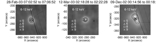
Figure 1.: Three examples of flare position finding. Positions are found from back-projection images of each event integrated over 4 minutes around the peak of the flare (in the 6–12 keV band). Images were created using detectors 5, 6, 8, and 9 individually (detector 7 has little sensitivity at low energies). For each image, a paraboloid was fit to the maximum in the image. Here, individual detector positions are shown overlaid on a representative back-projection image with 60%, 70%, 80%, 90% contours. (Left) An unresolved flare where positions from each detector agree. (Center) An unresolved flare where the flare position from detector 9 disagrees with the others due to the flare’s proximity to the spin axis. (Right) A resolved flare where positions from each detector disagree with each other since each detector resolves different sizes of the source. fig:pos˙finding

Here, positions were redetermined for each microflare. Positions were found through back projection images of each event integrated over 4 minutes around the peak time in the energy ranges, 4–10, 10–15, and 15–30 keV. The median nonthermal low energy cutoff for microflares was previously found to be 12 keV (Hannah et al., 2008), therefore the lowest energy band is dominated by thermal emission while the highest energy range is likely nonthermal. Images were created using detectors 5, 6, 8, and 9 individually (detector 7 has little sensitivity at low energies and was excluded). The angular resolutions are 20.4, 35.3, 105.8, 183.2 arcseconds, for detectors, 5, 6, 8, 9, respectively (Smith et al., 2002). For each image, a paraboloid was fit to the maximum in the image returning an interpolated flare position with errors (see Figure fig:pos_finding for examples).

The median flare loop length and width for microflares have been found to be 32 and 11 arcseconds, respectively (Hannah et al., 2008). This implies that detectors 6 and above may not resolve flare loops and should provide centroid positions that agree with each other. This fact provides a necessary cross check since it is not straightforward to algorithmically determine whether centroid locations which disagree between detectors are due to a resolved source or a noisy image. In order to include only those flares with confirmed positions, results from detectors 5, 6, 8, and 9 were compared. Those events with a standard deviation in position greater than 5 arcseconds (half of the median flare loop width) were excluded. This reduced the number of events from 25,006 to 8,503 for the 4–10 keV energy range. Detector 9 positions were found to differ significantly from other detectors. This is likely due to the fact that detector 9 has the coarsest resolution and is therefore most often affected by the spin axis (where imaging is difficult). The average location of the spin axis is around $[250,-100]$ arcsec (Christe et al., 2008), therefore flares on the west limb are 4 times the resolution of detector 9 away from the spin axis and should be largely unaffected. The final dataset now using detectors 5, 6, and 8 includes 14,750 events for 4–10 keV, 5,829 for 10–15 keV, and 1,452 for 15–30 keV. The flare positions can be seen in Figure fig:positions. Errors in the fitted centroids are small for all detectors. The average error in flare positions for detector 5 is 0.68 arcsec. These errors are smaller than the difference in positions between detectors, therefore the standard deviation of the set of positions is used as the error instead.

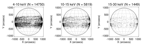
Figure 2.: The locations of RHESSI microflares from the RHESSI microflare list (Christe et al., 2008) re-evaluated using back projections images from detectors 5, 6, and 8 and averaging the positions from each. Those events with a standard deviation in position greater than 5 arcseconds were excluded. Flare positions are concentrated in the active region bands and near the limb. A lack of events can clearly be seen in the 4–10 keV positions around $[250,-100]$ arcsec, the average location of the spin axis, where imaging is difficult (Christe et al., 2008). fig:positions

3 Discussion

sec:discussion

Observations of solar source positions are a convolution of the radial source height and the spherical shape of the Sun. It is therefore difficult to determine the absolute height above the photosphere for individual events. In spherical coordinates, the relevant variables are the azimuthal angle, $\theta$ (or $\eta$, the longitude), the polar angle, $\phi$ ($\phi=\pi/2-\delta$ where $\delta$ is latitude), and the radius, $r$, which is related to the source height, $h$, by $r=R_{\odot}+h$ where $R_{\odot}$ is the solar radius. The position of an event is fully described by $(r,\eta,\phi)$. At the Earth, the only observable quantity is the two dimensional projection ($X=(R_{\odot}+h)\sin(\eta)\cos(\delta)$, $Y=(R_{\odot}+h)\sin(\delta)$) of this vector. The height of a source is easiest to observe at the limb where projection effects are small. In order to isolate the limb, we first define the radial distance of the source from the center of the solar disk as the projected source radius, $\rho=\sqrt{X^{2}+Y^{2}}$, which is related to the coordinate variables through the following equation,

$$\rho=(R_{\odot}+h)\sqrt{\sin(\eta)^{2}\cos(\delta)^{2}+\sin(\delta)^{2}}.\ilabel{eq:rho}$$ (1)

The measured projected source radius distribution for each energy band can be seen in Figure  fig:obs_distribution. Most events are observed to occur above the limb.

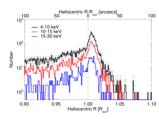
Figure 3.: fig:obs˙distribution The radial distribution of observed flare positions near the limb for each energy range (4–10 keV, 10–15 keV, 15–30 keV). The positions were corrected for the apparent size of the Sun and the solar B angle. The dashed line represents the optical solar limb. Positions are found to be concentrated at the limb with a peak at a heliocentric radius of approximately 1.005$R_{\odot}$ and a steeply falling distribution above the limb. The peak in the distribution above the limb is an artifact due to partially-occulted sources.

Generally none of the variables on the right-hand side of equation eq:rho are known. Yet if the distributions for each variable ($g(\eta),g(\delta),g(h)$) is known then the distribution of the projected source radius, $g(\rho)$, can be determined. Assuming all events are on the equator ($g(\delta)=0$), have identically zero height ($g(h)=0$), and are uniformly distributed in longitude, the distribution function for $\rho$ is given by

$$g(\rho)=\frac{A}{\sqrt{1-(\rho/R_{\odot})^{2}}}\ilabel{eq:simplemodel}$$ (2)

where A is a normalization constant. Generally, deriving an analytical solution for $g(\rho)$ is impossible, therefore a forward fit model was developed. The model takes as input a source height distribution, $g(h)$, a longitude and latitude distribution and generates random vectors ($h$, $\eta$, $\delta$). The longitude distribution is assumed to be uniform while random latitudes are generated based on the observed microflare latitude distribution (see Christe et al., 2008). These random vectors are then projected onto the two dimensional visible solar disk as ($X$, $Y$) excluding those that are occulted. The source projected radius, $\rho$, is then calculated for each event and the distribution, $g(\rho)$, can be compared with the measured distribution to determine the height distribution, $g(h)$.

In this study, two height model distributions are considered; an exponential distribution defined by $g(h)=A\ \mathrm{exp}(\frac{-h}{\lambda})$ and a power-law distribution, $g(h)=Ah^{-\alpha}$. These two models were chosen for their mathematical simplicity following the example of Catalano and van Allen (1973) and are not necessarily physically motivated.

The discussion so far has assumed point sources. Finite source size should have no effect on the projected radial distribution for sources well above the photosphere ($\rho>\sigma_{size}$). Those sources whose maxima are behind the limb yet are within $\sim$$\sigma_{size}$ will show emission truncated by the solar limb. RHESSI imaging of a partially occulted source will be “blurred” and show a source maximum above the limb whose height is dependent on the detector resolution. This effect places a minimum threshold below which the height of occulted sources cannot be accurately determined by RHESSI and is the reason for the maximum in the observed radial distribution. For detector 5, 6, and, 8 the height of the peak in the radial distribution was found to be 5.0, 5.3, and 6.7 arcsec above the limb, respectively. Height determination for sources as close to the limb as these values should be investigated carefully in order to determine whether they are occulted. In the following analysis, both height models include an unphysical minimum cutoff height, $h_{0}$, to model this effect. Using only unresolved sources, as is done here, is unlikely to affect the shape of the height distribution though there may be an affect on the minimum source height value if the source height is related to the source size.

4 Analysis

Using the method described above, the height model distributions were fit to the observed distribution through multiple Monte Carlo runs. Best fit parameters were determined through a grid search for the minimum in the $\chi^{2}$ space. The number of simulated events required for the Monte Carlo simulation were chosen in order to make the variance in the minimum smaller than the errors as determined by the contours of the $\chi^{2}$-space while maintaining an acceptable computation time. For the exponential height model, in the 4–10 keV energy range, the scale height, $\lambda$, was found to be $6.1\pm 0.3$ Mm and the minimum height, $h_{0}$, is $5.7\pm 0.3$ with a reduced $\chi^{2}$ of $1.06$. The fit results can be seen in Figure fig:obs_fit. The authors would like to point out the presence of a step-like structure at $\approx 0.96R_{\odot}$. This feature is statistically significant and is most prominent in the eastern hemisphere. Its cause is unknown to the authors but it does not affect the results presented here. The fit results disagree with those found by Catalano and van Allen (1973) who found a scale height of $11\pm 3$ Mm in the 1–6 keV range though Aschwanden, Brown, and Kontar (2002) concluded that most past height measurements have large systematic systematic errors. H$\alpha$ flare positions, which Catalano and van Allen (1973) depends on, have an associated accuracy of 1 heliographic degree (or 12 Mm). Analyzing the study by Matsushita et al. (1992), which similarly depend on $H\alpha$ positions, Aschwanden, Brown, and Kontar (2002) required a correction factor of $-6.8$ Mm which, if applied to Catalano and van Allen (1973), would lead to agreement with the results found here.

  

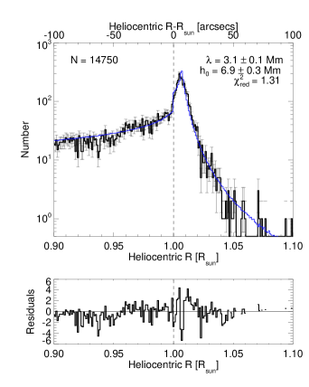
Figure 4.: The radial distribution of observed flare positions near the limb in the 4–10 keV (black) energy bands. The dashed line represents the optical solar limb. (Left) The best fit assuming an exponential height distribution is overlaid in blue. The scale and minimum height were found to be $6.1\pm 0.3$ Mm and $5.7\pm 0.3$ Mm, respectively. The exponential fit captures the overall behavior of the data though underestimates the number of events at large heliocentric radii. (Right) The best fit assuming a power-law height distribution. The power-law index and minimum height were found to be $3.1\pm 0.1$ Mm and $6.9\pm 0.3$ Mm, respectively. The power-law height distribution fit is worse than the exponential height distribution as measured by the reduced $\chi^{2}$ but better captures the events at large heliocentric radii. fig:obs˙fit

Fits were also performed for the 10–15 keV and 15–30 keV energy range. Though those results have poorer statistics, they agree with the 4–10 keV fit to within $1\sigma$. These results are consistent with past observations of thermal loops such as those of Ohki et al. (1983) and Takakura et al. (1986).

The power-law height distribution was also fit to the data for each energy channel. The power-law index, $\alpha$, was found to be $-3.1\pm 0.1$ with a minimum height, $h_{0}$, of $6.9\pm 0.3$ Mm, similar to the minimum height found in the exponential height model, and a reduced $\chi^{2}$ of $1.31$. Again, the results at the higher energies were found to agree. Both the exponential and power-law height models fit the data well with a small reduced $\chi^{2}$. The exponential fit was found to fit the data close to the limb better than the power-law model. This fact explains the lower value of $\chi^{2}$ for the exponential fit. On the other hand, the power-law fit better captures the tail of events at high heliocentric radius.

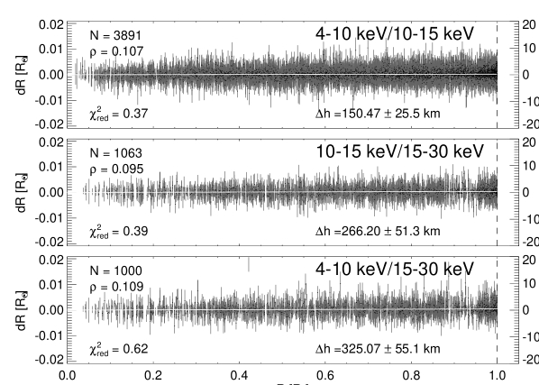
Figure 5.: The displacement versus projected radial position for each energy range. A fit to the data yields the average height difference between energy ranges (white line). The errors bars represent the standard deviation of the positions from different detectors. The average height differences are small, $\Delta h_{4-10,10-15\ \mathrm{keV}}=150\pm 25$ km, $\Delta h_{10-15,15-30\ \mathrm{keV}}=270\pm 51$ km, and $\Delta h_{4-10,15-30\ \mathrm{keV}}=320\pm 55$ km where lower energies are at larger heights. The results are found to be self-consistent since $\Delta h_{4-10,15-30\ \mathrm{keV}}=\Delta h_{4-10,10-15\ \mathrm{keV}}+\Delta h_{10-15,15-30\ \mathrm{keV}}$. fig:matsushita

To better compare the source heights between different energies, a method developed by Matsushita et al. (1992) and more recently applied by Sato et al. (2006) is appropriate here. Assuming that multiple pairs of points lie on either one of two concentric spheres with different radii, then the relationship between the projected radial positions and the length of the displacement vectors between each pair of points is related to the difference in radius (or height, $h$) between the two spheres. This method, by design, ignores those events observed above the limb and is therefore not sensitive to the problem of partially occulted sources. Figure fig:matsushita displays this relationship for each energy range. The errors bars represent the standard deviation of the positions from different detectors. The fitted height differences were found to be small; $\Delta h_{4-10,10-15\ \mathrm{keV}}=150\pm 25$ km, $\Delta h_{10-15,15-30\ \mathrm{keV}}=270\pm 51$ km, and $\Delta h_{4-10,15-30\ \mathrm{keV}}=320\pm 55$ km where lower energies are at larger heights. These results are found to be self-consistent since it must be that $\Delta h_{4-10,15-30\ \mathrm{keV}}=\Delta h_{4-10,10-15\ \mathrm{keV}}+\Delta h_{10-15,15-30\ \mathrm{keV}}$. The reduced $\chi^{2}$ for all of the fits are less than one which suggests that the errors, which here represent the standard deviation in the set of detector positions, are too large. This may indicate that source structure is being resolved. Comparing to previous uses of this method, it is found that the height differences are small compared to results by both Matsushita et al. (1992) and Sato et al. (2006). The absolute heights in each energy band suggests that images in all energy bands are dominated by thermal sources.

In order to better interpret the fitted height distribution, we used the potential-field source-surface (PFSS) to model (non-flaring) magnetic loops. This model calculates the magnetic field in the corona using photospheric magnetic field observations (SOHO/MDI) assuming that there are no currents ($\nabla\times B=0$). This model was initially developed by Altschuler and Newkirk (1969) and Schatten, Wilcox, and Ness (1969), and later refined by Hoeksema (1984) and Wang and Sheeley (1992). The PFSS model, through its assumption of zero current, models the lowest energy state of the (non-flaring) corona. It is, therefore, not an accurate model of the actual corona below $\sim$1.6 solar radii yet it provides a useful theoretical “base” corona to compare with.

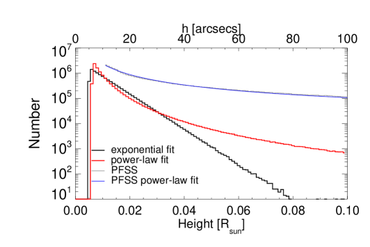
Figure 6.: The height distribution models compared. The fitted exponential (black) and power-law (red) models ($\alpha=3.1\pm 0.1$) are shown. The two models diverge significantly above 0.05$R_{\odot}$. The PFSS loop height distribution is also shown along with a power-law fit ($\alpha_{PFSS}=-1.4\pm 0.12$). The PFSS loop distribution has a much harder distribution than the measured distribution which may be due to the energization process of the corona. fig:height˙distribution

Using the standard PFSS software developed by M. DeRosa (see Schrijver and De Rosa, 2003) and distributed with SolarSoft, the PFSS height model was calculated from 0.01 to 2.0$R_{\odot}$. In order to get an accurate representative corona, the PFSS model was calculated every thirty days from March 2005 to March 2007, the time range of the RHESSI microflare list. Magnetic field lines were traced for each date and the maximum height for every (closed) loop was determined. From this the PFSS loop height distribution was then determined and each was fit with a power-law. The distribution shown here is the average for every date. The power-law index, $\alpha_{PFSS}$, of the average distribution was found to be $-1.4\pm 0.12$. The error in the power-law index represents the standard deviation of the set of fit values for individual dates. The distribution of PFSS loop-top heights can be seen in Figure fig:height_distribution compared with the power-law and exponential fits to the microflare height distribution. The PFSS height distribution was found to be much less steep than the power-law fit to the data with a difference in power-law index of $1.8\pm 0.16$ which implies that the ensemble of potential loops contain more large loops than the observed distribution. A soft loop height distribution may be a signature of the energization process of the corona.

5 Conclusions

sec:conclusion

Taking advantage of the large dataset provided by the RHESSI microflare list, the height distribution of HXR microflares was determined. The distribution of HXR (4-10 keV) source heights was found to be well fit by an exponential distribution with a scale height of $6.1\pm 0.3$ Mm. A power-law height distribution with a negative power-law index of $3.1\pm 0.1$ was also found to be consistent with the data though a worse fit. The minimum observable height due to partially occulted sources was found to be $5.7\pm 0.3$ Mm. The value of the heights found here suggests that they are thermal loop sources. Thermal loops are frequently assumed to be semicircular loops. The center of mass of a semicircular loop is located 36% below the loop-top therefore the minimum observable loop-top height may be as low as 7.7 Mm. In practice, RHESSI images of loops do not usually show the base of the loop, therefore it is likely that this is an overestimate.

The height distributions were compared to the loop height distribution as determined by a potential field model (PFSS). It was found that the measured flare height distribution was much steeper than the PFSS magnetic loop heights (difference in the power-law index of $\sim$1.8) meaning the ensemble of potential loops contain many more large loops compared to the height distribution found here. Observations of rising post-flare loops in EUV suggest that the flare loop distribution may relax to the PFSS distribution as energy is dissipated. In order for the observed distribution to transition to the potential distribution small flare loops must rise faster than large flare loops. It must also be true that an energized corona suppresses large loops.

The height distribution for different energies (4–10 keV, 10–15 keV, 15–30 keV) were found to agree within statistical uncertainties. More sensitive analysis showed that the difference in the average height were small, $\Delta h_{4-10,10-15\ \mathrm{keV}}=150\pm 25$ km, $\Delta h_{10-15,15-30\ \mathrm{keV}}=270\pm 51$ km, where lower energies are at greater heights. This suggests that emission in each energy range should be interpreted as from thermal flare loops.

The minimum observable height found, $h_{0}=6.3\pm 0.3$ Mm, introduced by partially-occulted flares, suggests that investigations of flares at the limb should be mindful of this limitation whereby limb sources may appear at higher altitudes if they are partially behind the limb. Such events should be detectable by the fact that images with different detectors will show positions which move away from the limb as a function of resolution. It should also be possible to detect partially-occulted flares through the visibilities in the highest resolution detectors which should have unusually large amplitudes for directions parallel to the limb.

Acknowledgements

This work was partially supported under NASA grant NAS5-98033 and NNM05ZA12H. The authors would like to thank the referee for input which has greatly improved this paper.

References

- Altschuler and Newkirk (1969) Altschuler, M.D., Newkirk, G.: 1969, Sol. Phys. 9, 131.
- Aschwanden, Brown, and Kontar (2002) Aschwanden, M.J., Brown, J.C., Kontar, E.P.: 2002, Sol. Phys. 210, 383.
- Aschwanden, Schwartz, and Alt (1995) Aschwanden, M.J., Schwartz, R.A., Alt, D.M.: 1995, ApJ 447, 923.
- Catalano and van Allen (1973) Catalano, C.P., van Allen, J.A.: 1973, ApJ 185, 335.
- Christe et al. (2008) Christe, S., Hannah, I.G., Krucker, S., McTiernan, J., Lin, R.P.: 2008, ApJ 677, 1385.
- Hannah et al. (2008) Hannah, I.G., Christe, S., Krucker, S., Hurford, G.J., Hudson, H.S., Lin, R.P.: 2008, ApJ 677, 704.
- Hoeksema (1984) Hoeksema, J.T.: 1984, Structure and evolution of the large scale solar and heliospheric magnetic fields. PhD thesis, Stanford Univ., CA..
- Hurford et al. (2002) Hurford, G.J., Schmahl, E.J., Schwartz, R.A., Conway, A.J., Aschwanden, M.J., Csillaghy, A., Dennis, B.R., Johns-Krull, C., Krucker, S., Lin, R.P., McTiernan, J., Metcalf, T.R., Sato, J., Smith, D.M.: 2002, Sol. Phys. 210, 61.
- Kane (1983) Kane, S.R.: 1983, Sol. Phys. 86, 355.
- Kane et al. (1979) Kane, S.R., Anderson, K.A., Evans, W.D., Klebesadel, R.W., Laros, J.: 1979, ApJ 233, 151.
- Kontar, Hannah, and MacKinnon (2008) Kontar, E.P., Hannah, I.G., MacKinnon, A.L.: 2008, A&A 489, 57.
- Kontar et al. (2010) Kontar, E.P., Hannah, I.G., Jeffrey, N.L.S., Battaglia, M.: 2010, ApJ 717, 250.
- Matsushita et al. (1992) Matsushita, K., Masuda, S., Kosugi, T., Inda, M., Yaji, K.: 1992, PASJ 44, 89.
- Ohki et al. (1983) Ohki, K., Takakura, T., Tsuneta, S., Nitta, N.: 1983, Sol. Phys. 86, 301.
- Sato et al. (2006) Sato, J., Matsumoto, Y., Yoshimura, K., Kubo, S., Kotoku, J., Masuda, S., Sawa, M., Suga, K., Yoshimori, M., Kosugi, T., Watanabe, T.: 2006, Sol. Phys. 236, 351.
- Schatten, Wilcox, and Ness (1969) Schatten, K.H., Wilcox, J.M., Ness, N.F.: 1969, Sol. Phys. 6, 442.
- Schrijver and De Rosa (2003) Schrijver, C.J., De Rosa, M.L.: 2003, Sol. Phys. 212, 165.
- Smith et al. (2002) Smith, D.M., Lin, R.P., Turin, P., Curtis, D.W., Primbsch, J.H., Campbell, R.D., Abiad, R., Schroeder, P., Cork, C.P., Hull, E.L., Landis, D.A., Madden, N.W., Malone, D., Pehl, R.H., Raudorf, T., Sangsingkeow, P., Boyle, R., Banks, I.S., Shirey, K., Schwartz, R.: 2002, Sol. Phys. 210, 33.
- Takakura et al. (1986) Takakura, T., Tanaka, K., Nitta, N., Kai, K., Ohki, K.: 1986, Sol. Phys. 107, 109.
- Tsuneta et al. (1984) Tsuneta, S., Takakura, T., Nitta, N., Makishima, K., Murakami, T., Oda, M., Ogawara, Y., Kondo, I., Ohki, K., Tanaka, K.: 1984, ApJ 280, 887.
- Wang and Sheeley (1992) Wang, Y., Sheeley, N.R. Jr.: 1992, ApJ 392, 310.