The Cool Accretion Disk in ESO 243-49 HLX-1: Further Evidence of an Intermediate Mass Black Hole

Abstract

With an inferred bolometric luminosity exceeding $10^{42}$ $\rm erg\;s^{-1}$, HLX-1 in ESO 243-49 is the most luminous of ultraluminous X-ray sources and provides one of the strongest cases for the existence of intermediate mass black holes. We obtain good fits to disk-dominated observations of the source with BHSPEC, a fully relativistic black hole accretion disk spectral model. Due to degeneracies in the model arising from the lack of independent constraints on inclination and black hole spin, there is a factor of 100 uncertainty in the best-fit black hole mass $M$. Nevertheless, spectral fitting of XMM-Newton observations provides robust lower and upper limits with $3000M_{\odot}\lesssim M\lesssim 3\times 10^{5}M_{\odot}$, at 90% confidence, placing HLX-1 firmly in the intermediate-mass regime. The lower bound on $M$ is entirely determined by matching the shape and peak energy of the thermal component in the spectrum. This bound is consistent with (but independent of) arguments based solely on the Eddington limit. Joint spectral modelling of the XMM-Newton data with more luminous Swift and Chandra observations increases the lower bound to $6000M_{\odot}$, but this tighter constraint is not independent of the Eddington limit. The upper bound on $M$ is sensitive to the maximum allowed inclination $i$, and is reduced to $M\lesssim 10^{5}M_{\odot}$ if we limit $i\lesssim 75^{\circ}$.

1. Introduction

Ultraluminous X-ray sources (ULXs) are extragalactic X-ray sources whose luminosities match or exceed the Eddington luminosity for accretion onto a 10 $M_{\odot}$ black hole (BH). It is thought that the most luminous objects in this class may harbor BHs with masses in the $100$ to $10^{5}M_{\odot}$ range (intermediate mass black holes or IMBHs). BHs in this mass range are of particular interest because our current understanding of stellar evolution suggests they could not be formed by the collapse of a single massive star in the current epoch of star formation (e.g., Belczynski et al., 2010, and references therein). The strongest support for the IMBH interpretation is founded on theoretical arguments that BH accretion flows cannot radiate significantly above the Eddington luminosity. If this argument holds, the most luminous ULX sources, which exceed $10^{40}$ $\rm erg\;s^{-1}$, must host IMBHs. Alternatively, if real accretion flows are capable of radiating significantly above the Eddington limit or their emission is strongly beamed (King et al., 2001), these sources might contain BHs of only a few tens of solar masses. BHs in this lower mass range have been identified through dynamical studies of X-ray binaries in the Milky Way and other Local Group galaxies (Remillard & McClintock, 2006). These sources can easily be explained by the theory of stellar evolution and collapse.

Cool thermal components found in the spectra of some ULX sources provide additional support for the IMBH interpretation. Due to the scaling of the characteristic gravitational radius and luminosity with mass, accretion disks radiating at a fixed fraction of the Eddington luminosity will tend to have lower maximum effective temperatures for larger masses if the inner radius of the accretion flow scales with the gravitational radius of the BH (Shakura & Sunyaev, 1973; Novikov & Thorne, 1973). In many luminous ULXs, fits with multicolor disk blackbody models favor relatively cool disks (e.g., Miller et al., 2003, 2004a, 2004b). However, the disk component in many of these spectral fits only accounts for a small or modest fraction of the bolometric power (see e.g. Socrates & Davis, 2006; Soria et al., 2009), which is instead dominated by a power law component, generally thought to be inverse Compton scattering of disk photons by hot electrons. If the majority of the emission originates in the hard component, it is no longer clear that the thermal component is associated with emission from near the inner edge of the disk (as opposed to larger radii), and the argument that a larger emitting area follows from a larger gravitational radius (i.e. a large mass) is weakened.

Making a convincing argument for an IMBH on the basis of spectral fits requires observations in which a thermal component dominates the bolometric emission. However, such observations appear to be rare for ULXs with luminosities $\gtrsim 10^{40}$ $\rm erg\;s^{-1}$ (Socrates & Davis, 2006; Berghea et al., 2008; Soria & Kuncic, 2008; Feng & Kaaret, 2009; Soria et al., 2009). Most luminous ULXs are observed in a power-law dominated state resembling the hard state or steep powerlaw state of BH X-ray binaries (McClintock & Remillard, 2006), although there are also suggestions that this may be a new mode of super-Eddington accretion (e.g., Socrates & Davis, 2006; Gladstone et al., 2009). Exceptions may include recent observations of M82 X-1 (Feng & Kaaret, 2010) and HLX-1 in ESO 243-49, hereafter referred to simply as HLX-1 (Farrell et al., 2009), in which the spectra of these sources appear to be dominated by a thermal component.

In this work we focus on HLX-1, an off-nuclear X-ray source in the galaxy ESO 243-49, which reaches luminosities in excess of $10^{42}$ $\rm erg\;s^{-1}$ (Farrell et al., 2009; Godet et al., 2009; Webb et al., 2010). The source has been observed a number of times with XMM-Newton, Swift, and Chandra, displaying long term spectral variability that is consistent with state transitions in Galactic X-ray binaries (Godet et al. 2009; Servillat et al., in preparation). This large luminosity is contingent on its placement in ESO 243-49. Soria et al. (2010) have argued that the X-ray spectrum could plausibly be explained as a foreground neutron star in the Milky Way. However, based on recent spectroscopic observations with the Very Large Telescope, Wiersema et al. (2010) identify H$\alpha$ emission coincident with HLX-1 at a very similar redshift to that of the host galaxy, placing the source firmly in ESO 243-49.

For fitting the spectrum of HLX-1, we use BHSPEC (Davis et al., 2005; Davis & Hubeny, 2006), a relativistic accretion disk spectral model, which has been implemented as a table model in XSPEC (Arnaud, 1996). The major advantage of this model is that the spectrum of the emission at the disk surface is not assumed to be blackbody, but is instead computed directly using TLUSTY (Hubeny & Lanz, 1995), a stellar atmospheres code which has been modified to model the vertical structure of accretion disks (Hubeny, 1990; Hubeny & Hubeny, 1998). The BH mass (and spin) are parameters of the model and are directly constrained by spectral fitting.

BHSPEC, alone or in concert with KERRBB (Li et al., 2005), has been used to fit numerous Galactic BH X-ray binaries. For observations in which the thermal component dominates, it provides a good fit and reproduces the spectral evolution as luminosity varies (e.g., Shafee et al., 2006; Davis et al., 2006; Steiner et al., 2010, and references therein). However, the mass range covered by the BHSPEC models used in those works was below the IMBH range. BHSPEC models in the IMBH regime were generated by Hui et al. (2005). With these models, Hui & Krolik (2008) obtained good fits and found best-fit BH masses in the 23-73 $M_{\odot}$ range for five of the six ULX sources in their sample, all of which were at least an order-of-magnitude lower in luminosity than HLX-1. We have extended our own version of the BHSPEC model into the IMBH regime and have used these models for the analysis presented here, but the methods are identical to those employed by Hui & Krolik (2008).

This work is organized as follows: We briefly describe the BHSPEC model and discuss our data selection in Section 2. We summarize the main results of our spectral analysis in Section 3, and provide a more thorough discussion of our constraints in Section 4. We summarize and conclude in Section 5.

2. Methods

2.1. Spectral Models

In this work, we focus exclusively on the BHSPEC model. We are motivated by the observational evidence of a thermally dominant soft X-ray component in the spectra of HLX-1 considered here and the similarity of these spectra to those observed in Galactic BH X-ray binaries. Hence, we assume from the outset that the emission is from a radiatively efficient, thin accretion disk, and derive constraints on the parameters of interest, most importantly the BH mass, $M$. We refer readers interested in comparisons with other models to Godet et al. (in preparation), which fits a wider array of models and attempts to differentiate between various interpretations.

In addition to $\log M$, the BHSPEC model has 4 fit parameters: a normalization, the BH spin $a_{*}$, the cosine of the inclination $i$, and the log of the Eddington ratio $\ell=L/L_{\rm Edd}$, where $L_{\rm Edd}=1.3\times 10^{38}(M/M_{\odot})\rm\;erg\;s^{-1}$ is the Eddington luminosity. The normalization can be fixed using the known distance to the source of $D\sim 95$ Mpc, leaving 4 parameters to fit. We have computed models for $\log\ell=-1.5$ to 0, $\log M/M_{\odot}=3.25$ to 5.5, $\cos i=0$ to 1, and $a_{*}=-1$ to 0.99. We assume a Shakura & Sunyaev (1973) stress parameter $\alpha=0.01$, but discuss the implications of this choice in Section 4.

Although the spectra under consideration are thermally dominated, there is a tail of emission at high energies which is not accounted for by BHSPEC. We model this emission with SIMPL (Steiner et al., 2009), which adds two free parameters: the power law index $\Gamma$ and the fraction of scattered photons $f_{\rm sc}$ relative to the BHSPEC model. Photoelectric absorption by neutral gas along the line of sight is accounted for by the PHABS model in XSPEC. We leave the neutral hydrogen column $N_{\rm H}$ free, adding a single additional parameter.

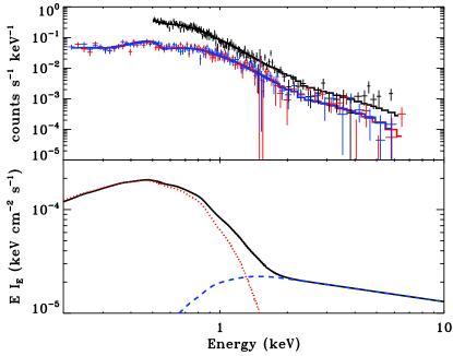
Figure 1.— XMM2 spectrum (top) and best-fit unabsorbed model (bottom) versus energy for $\cos i=1$ in Table 1. The top panel shows the observed count rate and best-fit model (with absorption) for the EPIC pn (black), MOS1 (red) and MOS2 (blue) data. The bottom panel shows the best-fit total model (solid, black), BHSPEC component (dotted, red), and SIMPL component (dashed, blue) with absorption removed.

Table 1Best-FitXMM-Newton Parameters

$\cos i$	$a_{*}$	$\log M$	$\log\ell$	$N_{H}$	$\Gamma$	$f_{\rm sc}$	$\chi^{2}$/d.o.f.
$0$	$0.23^{+0.42}_{-0.04}$	$4.79^{+0.10}_{-0.05}$	$0.00^{+0}_{-0.22}$	$1.5^{+1.2}_{-1.0}$	$2.37^{+0.39}_{-0.28}$	$0.108^{+0.044}_{-0.027}$	$332/328$
$0.25$	$0.99^{+0}_{-0.07}$	$5.07^{+0.07}_{-0.20}$	$-1.19^{+0.27}_{-0.01}$	$2.6^{+1.0}_{-1.2}$	$2.72^{+0.40}_{-0.36}$	$0.142^{+0.072}_{-0.043}$	$339/328$
$0.5$	$0.99^{+0}_{-0.04}$	$4.78^{+0.08}_{-0.19}$	$-0.97^{+0.09}_{-0.04}$	$2.9^{+1.2}_{-1.2}$	$2.54^{+0.39}_{-0.46}$	$0.108^{+0.053}_{-0.041}$	$340/328$
$0.75$	$-0.93^{+1.92}_{-0.07}$	$3.72^{+0.96}_{-0.04}$	$-0.16^{+0.02}_{-0.56}$	$2.5^{+1.2}_{-1.0}$	$2.28^{+0.45}_{-0.35}$	$0.080^{+0.030}_{-0.024}$	$338/328$
$1$	$0.51^{+0.48}_{-1.51}$	$3.83^{+0.31}_{-0.32}$	$-0.37^{+0.22}_{-0.09}$	$2.5^{+1.1}_{-1.0}$	$2.31^{+0.39}_{-0.39}$	$0.085^{+0.044}_{-0.035}$	$336/328$
$0.94^{+0.06}_{-0.06}$	$-1$	$3.61^{+0.18}_{-0.06}$	$-0.16^{+0.03}_{-0.02}$	$1.9^{+1.3}_{-1.1}$	$2.37^{+0.41}_{-0.37}$	$0.091^{+0.050}_{-0.029}$	$336/328$
$0.03^{+0.04}_{-0.00}$	$0$	$4.70^{+0.08}_{-0.11}$	$0.00^{+0}_{-0.07}$	$2.1^{+1.2}_{-0.9}$	$2.38^{+0.43}_{-0.33}$	$0.099^{+0.043}_{-0.022}$	$334/328$
$0.00^{+0.03}_{-0}$	$0.7$	$4.89^{+0.08}_{-0.07}$	$-0.26^{+0.03}_{-0.08}$	$1.9^{+1.3}_{-1.1}$	$2.34^{+0.36}_{-0.34}$	$0.099^{+0.037}_{-0.026}$	$335/328$
$1.00^{+0}_{-0.16}$	$0.95$	$4.07^{+0.21}_{-0.07}$	$-0.43^{+0.03}_{-0.15}$	$2.8^{+1.1}_{-1.0}$	$2.24^{+0.40}_{-0.39}$	$0.073^{+0.038}_{-0.025}$	$337/328$

Note. — Parameters tabulated without errors were fixed during the fit. Errors are computed using $\Delta\chi^{2}=2.706$ (90% confidence for one parameter). Joint confidence contours are shown in Figures 2 and 3.

2.2. Data Selection

We begin with a collection of prospective disk dominated observations of HLX-1. This includes two observations with XMM-Newton (2004 November 23: XMM1; 2008 November 28: XMM2), two observations with Swift (2008 November 24: S1; 2010 August 30: S2), and one observation with Chandra (2010 September 6).

The XMM-Newton observations were performed with the three EPIC cameras in imaging mode with the thin filter. The two MOS cameras were in full-frame mode for both observations. The pn was operated in full frame mode for the first observation (Obs-Id: 0204540201) and small window mode for the second (Obs-Id: 0560180901). The data were reduced using the XMM-Newton Science Analysis System (SAS) v8.0 and event files were processed using the epproc and emproc tools. The event lists were filtered for event patterns in order to maximize the signal-to-noise ratio against non X-ray events, with only calibrated patterns (i.e. single to double events for the pn and single to quadruple events for the MOS) selected. Events within a circular region of radius 60” around the position of HLX-1 were extracted from the MOS data in both observations and from the pn data in the first observation. Background events were extracted for the same data from an annulus around the source position with an inner radius of 60” and an outer radius of 84.85”. As the pn was in the small window mode during the second observation, a smaller circular extraction region with a radius of 40” was used for extracting source events. Background events were in turn extracted from a circular region with radius 40” from a region the same distance from the center of the chip as HLX-1, which appeared to have a similar background level in the image. Source and background spectra were extracted in this way for each camera, with response and ancillary response files generated in turn using the SAS tools rmfgen and arfgen.

Although the MOS and pn spectra are consistent down to $\sim 0.5$ keV, below this boundary the pn spectrum deviates significantly, showing a sharp, absorption-like feature that is absent in the MOS spectra. Since this indicates a problem with the low energy response of the pn camera in this observation, we follow Farrell et al. (2009) and ignore channels with energies below 0.5 keV when fitting the pn spectrum. For the MOS spectra we fit channels with energies greater than 0.2 keV.

The Swift XRT data were processed using the tool XRTPIPELINE v0.12.3.4, as discussed in Godet et al. (2009). The Chandra ACIS-S data reduction is discussed in more detail in Servillat et al. (in preparation). Their modeling indicates that the data likely suffer from mild pile-up, so we include a pile-up model based on Davis (2001) in our spectral fits, following the guidelines in the Chandra ABC Guide to Pileup. The grade migration parameter (denoted by $\alpha$ in the guide, and not to be confused with the accretion disk stress parameter) was left as a free parameter in our initial fits. These fits generically favored the maximum allowed value of 1. Our best-fit BHSPEC parameters were mildly sensitive to variations in this $\alpha$, but $\alpha\sim 1$ yields results which are consistent with the S1 and S2 datasets. Hence we fixed $\alpha=1$ for subsequent analysis. The frame time was set to 0.8 s to match the observational setup, and all other parameters were left at their XSPEC defaults.

All spectra were rebinned to require a minimum of 20 counts per bin.

Using XSPEC (v12.6.0q), we fit each observation independently to determine its suitability for modeling with BHSPEC. Specifically, we evaluate the level of disk dominance for typical best-fit parameters. For both of the XMM-Newton observations, we fit all EPIC datasets (MOS1, MOS2, and pn) simultaneously. An additional hard X-ray component is necessary to obtain a good fit for these datasets. Fits with SIMPL typically find a best-fit scattering fraction $f_{\rm sc}\gtrsim 0.5$ for the XMM1 data and $f_{\rm sc}\lesssim 0.15$ for XMM2. These results are consistent with those of Farrell et al. (2009) who find an acceptable fit to the XMM1 data with an absorbed power-law, but require an additional soft component (modeled with DISKBB, Mitsuda et al., 1984) for the XMM2 data. Our fits suggest that the XMM1 spectrum is more typical of a steep power-law state, while the XMM2 spectrum is consistent with a thermally dominated state. A large $f_{\rm sc}$ in the fit with SIMPL is problematic for our accretion disk model, which does not account for the effects of irradiation by neighboring corona. Hence, we only report our results from the XMM2 analysis below. We note that the XMM1 data generally favor a best-fit $M$ that is higher than XMM2 for the same $i$. This yields a cooler disk model, consistent with the fact that more of the high energy flux is accounted for with the SIMPL component in these data. However, the joint confidence contours on $a_{*}$ and $M$ are much larger for the XMM1 data, so the best-fit values are still consistent with the XMM2 values at 90% confidence.

The Swift and Chandra observations caught the source at higher luminosities than the XMM2 observation, but the overall signal-to-noise is still lower because of the lower effective area of the Swift XRT and the short duration (10 ks) of the Chandra ACIS-S observation. Due to the lower signal-to-noise and stronger disk dominance, a suitable fit is provided by the (absorbed) BHSPEC model alone. The addition of the SIMPL model only provides a marginal improvement to the fit and the best-fit SIMPL parameters are poorly constrained. We also fit the combined S1 and S2 observations. In this case we tie all BHSPEC parameters together, except for $\ell$, which is allowed to vary independently for S1 and S2. Even for the combined dataset, we find a good fit with BHSPEC alone, and poor constraints on the SIMPL model parameters. Therefore, we do not include the SIMPL model in subsequent analysis of the combined S1 and S2 datasets or in our analysis of the Chandra data.

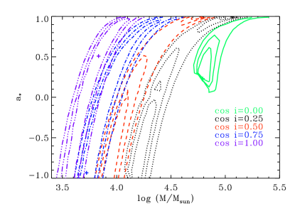
Figure 2.— Joint confidence contours of $a_{*}$ and $M$, assuming fixed inclination for the XMM2 data. Each set of contours is computed by fitting the BHSPEC model with fixed $\cos i=0$ (solid, green), 0.25 (dotted, black), 0.5 (dashed, red), 0.75 (dot-dashed, blue), or 1 (triple-dot-dashed, violet). The three contours in each set are $\Delta\chi^{2}=2.3$, 4.61, and 9.21, corresponding to 68%, 90%, and 99% joint confidence on $a_{*}$ and $\log M$.

3. Results

3.1. XMM-Newton Results

We first consider the XMM2 observation. The soft thermal component is largely characterized by only two parameters: the energy at which the spectrum peaks and the overall normalization. In practice, this leads to degeneracies in the best-fit parameters of BHSPEC (see e.g. Davis et al., 2006), unless all but two of the parameters can be independently constrained. Since we can only constrain $D$ independently, we will need to consider joint variation of the remaining parameters.

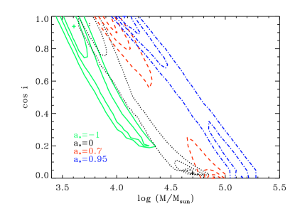
Figure 3.— Joint confidence contours for BH mass and inclination, assuming fixed BH spin, for the XMM2 observation. Each set of contours is computed by fitting the BHSPEC model with fixed $a_{*}=-1$ (solid, green), 0 (dotted, black), 0.7 (dashed, red), or 0.95 (dot-dashed, blue). The three contours in each set correspond to 68%, 90%, and 99% joint confidence on $\cos i$ and $\log M$.

For completeness, our best-fit parameters for various choices of $i$ or $a_{*}$ are summarized in Table 1. We find acceptable fits for all $i$. The best-fit model and data for $i=0$ are plotted in Figure 1. We report the 90% confidence interval for a single parameter, but due to the significant degeneracies in the model, the joint confidence contours better illustrate the actual parameter uncertainties. Hence they are the focus of this work.

Since $M$ and $a_{*}$ are of primary interest to us, we first examine their joint confidence contours, and consider the joint confidence of $M$ and $i$ in Section 4. For illustration, it is useful to consider several sets of contours for different choices of (fixed) $i$, leaving $\ell$ as a free parameter. These best-fit joint confidence contours are shown in Figure 2. We consider five choices for $\cos i$, evenly spaced from 0 to 1. Each set of contours has three curves corresponding to 68%, 90%, and 99% confidence. These are determined by the change in $\chi^{2}$ relative to the best-fit values listed in Table 1.

Even for fixed $i$, there is a clear correlation of $a_{*}$ and $M$. At 99% confidence, the entire range of $a_{*}$ ($-1<a_{*}<0.99$) is allowed, and the corresponding $M$ varies by a factor of 4-5 over this range. The only exception is for nearly edge on systems ($\cos i\sim 0$), for which low spins are disallowed. The correlation of best-fit $M$ with $i$ is very strong as well, consistent with previous modeling of other ULX sources (Hui & Krolik, 2008). This is illustrated more clearly in Figure 3, which shows the joint confidence contours of $M$ and $\cos i$ for fixed $a_{*}=-1$, 0, 0.7, and 0.95. The corresponding best-fit values are listed in Table 1. At fixed $a_{*}$, there is up to a factor of 10 change in $M$ as inclination varies from $0^{\circ}$ to $90^{\circ}$. The combined overall uncertainty in the mass is nearly a factor of 100.

Despite these degeneracies, we can still place a firm lower limit of $M\gtrsim 3000M_{\odot}$ on the mass of the BH in HLX-1. The limiting mass is obtained for the case of a maximally spinning BH with a counter-rotating disk viewed nearly face-on. An independent lower limit on the mass may be obtained under the assumption that the source luminosity does not exceed the Eddington limit. This gives the same answer, $M\gtrsim 3000M_{\odot}$, which is purely coincidental. At the high mass end, the limit we obtain from our fits is $M\lesssim 3\times 10^{5}M_{\odot}$, where the limiting value is obtained for nearly maximal spins in the case where disk rotation is spin-aligned and the system is viewed nearly edge on. However, edge on systems may be ruled out by the lack of X-ray eclipses if one assumes the accreting matter is provided by a binary companion. If one limits $i\lesssim 75^{\circ}$, one obtains $M\lesssim 10^{5}M_{\odot}$. The above limits on the mass place HLX-1 in the IMBH regime, though the very highest masses in our allowed range approach the lower end of the mass distribution inferred in active galactic nuclei (e.g., Greene & Ho, 2007).

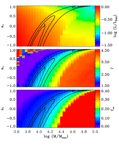
Figure 4.— From top to bottom, the best fit Eddington ratio, power law index, and scattering fraction in the $a_{*}-\log M$ plane, assuming $\cos i=0.5$. For comparison, we overplot three contours corresponding to 68%, 90%, and 99% joint confidence on $a_{*}$ and $\log M$.

We plot the variation of the other free parameters in Figure 4 for the specific example of $\cos i=0.5$. The variation of $\ell$ is the most interesting, as there are fairly clear correlations with $M$ and $a_{*}$. Following the best-fit contour, $\ell$ decreases as $M$ and $a_{*}$ increase. This correlation arises because $\ell$ has a role both in determining the location of the spectral peak as well as its overall normalization, a point we elaborate on in Section 4.

The bottom two panels show the variation of the SIMPL parameters. In contrast to $\ell$, these parameters tend to vary across (rather than along) the confidence contours, indicating that they are highly correlated with $\chi^{2}$. A similar behavior is present in the absorption column. For the best-fit values we find $N_{\rm H}\simeq 1-4\times 10^{20}\rm\;cm^{-2}$, $\Gamma\simeq 2.2-2.7$, and a scattered fraction $\lesssim 12\%$. The allowed $N_{\rm H}$ range is roughly equivalent to or slightly greater than the Galactic value ($1.7\times 10^{20}\;\rm cm^{-2}$, Kalberla et al., 2005). The ranges for the two SIMPL parameters are generally consistent with fits to the thermal state of Galactic BH binaries and confirm that the bolometric luminosity of the best-fit models is dominated by the BHSPEC component. For typical parameters within the confidence contours, the accretion disk accounts for 80-95% of the unabsorbed model luminosity from 0.3 to 10 keV. Comparison with Table 1 of Socrates & Davis (2006) shows that this is a much higher disk fraction than typically inferred in other bright ULXs, in which values 10-50% are more typical.

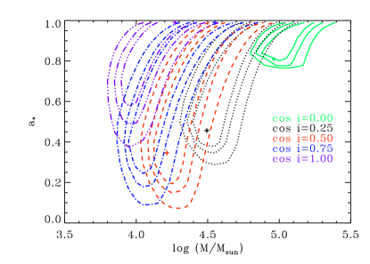
Figure 5.— Joint confidence contours of $a_{*}$ and $M$, assuming fixed inclination for the Swift data. Each set of contours is computed by fitting the BHSPEC model with fixed $\cos i=0$ (solid, green), 0.25 (dotted, black), 0.5 (dashed, red), 0.75 (dot-dashed, blue), or 1 (triple-dot-dashed, violet). The three contours in each set are $\Delta\chi^{2}=2.3$, 4.61, and 9.21, corresponding to 68%, 90%, and 99% joint confidence on $a_{*}$ and $\log M$.

3.2. Swift and Chandra Results

In Figure 5, we plot the best-fit joint confidence contours of $a_{*}$ and $M$ for the combined Swift (S1 and S2) data sets. Figure 6 is the corresponding plot for the Chandra dataset. As discussed in Section 2.2, we do not include a SIMPL component in fitting these datasets and we tie all the BHSPEC parameters together, except $\ell$, which is allowed to vary independently for each observation. The corresponding best-fit parameters are depicted with crosses and summarized in Tables 2 and 3, where $\ell_{1}$ and $\ell_{2}$ correspond to the S1 and S2 observations, respectively. The reduced $\chi^{2}$ for the Chandra data indicate a slightly poorer fit than with the XMM-Newton or Swift data. This is primarily due to narrow residuals near 0.6, 1.1 and 1.3 keV in fits to the ACIS-S data. Since these residuals are not highly significant and their presence does not significantly impact the best-fit BHSPEC parameters, we do not attempt to model them with additional components. Further discussion can be found in Servillat et al. (in preparation).

Table 2Best-Fit Swift Parameters

$\cos i$	$a_{*}$	$\log M$	$\log\ell_{1}$	$\log\ell_{2}$	$N_{H}$	$\chi^{2}$/d.o.f.
$0$	$0.81^{+0.18}_{-0.02}$	$4.96^{+0.30}_{-0.08}$	$-0.00^{+0}_{-0.68}$	$-0.05^{+0.03}_{-0.58}$	$3.2^{+3.1}_{-2.6}$	$58.3/75$
$0.25$	$0.46^{+0.46}_{-0.07}$	$4.49^{+0.38}_{-0.08}$	$-0.01^{+0.01}_{-0.92}$	$-0.06^{+0.03}_{-0.56}$	$5.1^{+3.1}_{-2.6}$	$59.6/75$
$0.5$	$0.35^{+0.64}_{-0.22}$	$4.21^{+0.63}_{-0.08}$	$-0.02^{+0.02}_{-0.54}$	$-0.06^{+0.04}_{-0.42}$	$5.3^{+3.5}_{-2.7}$	$59.8/75$
$0.75$	$0.99^{+0}_{-0.25}$	$4.54^{+0.09}_{-0.46}$	$-0.29^{+0.29}_{-0.04}$	$-0.33^{+0.31}_{-0.03}$	$5.3^{+3.5}_{-2.7}$	$58.9/75$
$1$	$0.99^{+0}_{-0.05}$	$4.27^{+0.05}_{-0.58}$	$-0.03^{+0.03}_{-0.06}$	$-0.08^{+0.08}_{-0.06}$	$7.0^{+3.2}_{-3.6}$	$58.5/75$

Note. — Parameters tabulated without errors were fixed during the fit. Errors are computed using $\Delta\chi^{2}=2.706$ (90% confidence for one parameter). Joint confidence contours are shown in Figure 5. In these joint fits to the S1 and S2 data sets all BHSPEC parameters are fit simultaneously to both spectra, except $\ell$ which is fit independently. Hence, $\ell_{1}$ and $\ell_{2}$ correspond to the S1 and S2 observations, respectively.

The Swift and Chandra data seem to place much tighter overall constraints on $a_{*}$ and $M$, with a minimum $a_{*}$ at each $i$. The overall minima of $M\sim 6000M_{\odot}$ for Swift) and and $M\sim 4000M_{\odot}$ for Chandra both correspond to $i=0^{\circ}$. Fits with retrograde accretion flows ($a_{*}<0$) are inconsistent with the Swift data and models with $a_{*}\lesssim-0.5$ are ruled out by the Chandra spectrum. For values of $a_{*}$ allowed by both data sets, the position of the confidence contours for a given $i$ are consistent with each other. They are also broadly consistent with the XMM2 results, although offset to slightly higher $M$. However, due to the lower signal-to-noise of the Swift and Chandra datasets, the range of allowed $M$ for a given $i$ is larger than in Figure 2.

The differences between the XMM-Newton fits and the Swift or Chandra results at low (negative) $a_{*}$ are driven primarily by the larger luminosities of the disk component in the Swift and Chandra observations. With the exception of nearly edge on systems ($\cos i=0$) we find $\ell<1$ within the 99% confidence contours in Figure 2. In the Swift and Chandra data, $\ell\geq 1$ is required for all $i$, at sufficiently low $a_{*}$. As we discuss further in Section 4, reductions in $a_{*}$ and $M$ must be offset by increases in $\ell$, but our models are capped at $\ell=1$, which sets a lower limit on the allowed $a_{*}$ and $M$ for a given choice of $i$. Hence, in contrast to the XMM2 observation, these tighter constraints depend strongly on the assumption that luminosity does not exceed the Eddington limit: $\ell\leq 1$.

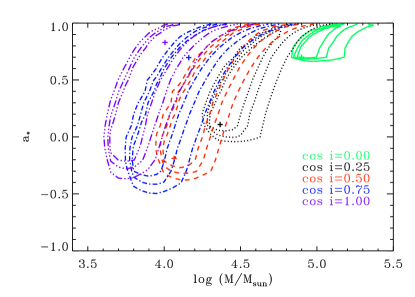
Figure 6.— Joint confidence contours of $a_{*}$ and $M$, assuming fixed inclination for the Chandra data. Each set of contours is computed by fitting the BHSPEC model with fixed $\cos i=0$ (solid, green), 0.25 (dotted, black), 0.5 (dashed, red), 0.75 (dot-dashed, blue), or 1 (triple-dot-dashed, violet). The three contours in each set are $\Delta\chi^{2}=2.3$, 4.61, and 9.21, corresponding to 68%, 90%, and 99% joint confidence on $a_{*}$ and $\log M$.

We also fit the combined Swift, Chandra and XMM-Newton datasets assuming no correction was needed to the relative effective area of the various instruments. In principle, a constant offset could be included based on cross-calibration analysis (e.g., Tsujimoto et al., 2011), but even without such a correction, we obtain good fits to the combined dataset. The range of allowed $a_{*}$ is similar to that found with the Swift data alone, but the width of the contours are comparable to those from the XMM2 fits plotted in Figure 2. At 99% confidence, the minimum allowed $M$ was about $6000M_{\odot}$, again for $i=0^{\circ}$ and $\ell=1$.

4. Discussion

Due to the complex interplay between the frequency and angular distribution of emitted photons in the rest frame of the flow, and the relativistic effects on the disk structure and radiation, it is preferable to use a self-consistent relativistic model to draw quantitative conclusions. Nevertheless, one can understand the basic trends and correlations with a simpler model, in which the relativistic effects are encapsulated into two parameters, similar in spirit to the pioneering work of Zhang et al. (1997).

4.1. A Minimal Relativistic Disk Model

To first approximation, thermal state disk spectra are characterized by only two parameters: a peak energy and an overall normalization. Indeed the popular DISKBB model (Mitsuda et al., 1984), with only two parameters, provides an acceptable fit to the soft thermal component of the XMM2 data (Farrell et al., 2009). Although we obtain all our constraints by fitting a relativistic accretion disk model directly to the spectrum, our fit results are easily understood in terms of these two constraints. These observables can be mapped onto a characteristic color temperature $T_{\rm obs}$ ($\approx T_{\rm in}$ from DISKBB), and since the distance $D$ is known, a characteristic luminosity $L_{\rm obs}$.

Table 3Best-Fit Chandra Parameters

$\cos i$	$a_{*}$	$\log M$	$\log\ell$	$N_{H}$	$\chi^{2}$/d.o.f.
$0$	$0.70^{+0.27}_{-0.05}$	$4.90^{+0.28}_{-0.04}$	$-0.01^{+0.01}_{-0.63}$	$0.0^{+2.0}_{-0.0}$	$48.4/38$
$0.25$	$0.11^{+0.85}_{-0.07}$	$4.37^{+0.37}_{-0.06}$	$-0.01^{+0.01}_{-0.73}$	$1.3^{+3.5}_{-1.3}$	$50.4/38$
$0.5$	$-0.19^{+1.18}_{-0.10}$	$4.06^{+0.77}_{-0.06}$	$0.00^{+0.00}_{-0.68}$	$1.8^{+4.0}_{-1.8}$	$50.1/38$
$0.75$	$0.70^{+0.29}_{-1.06}$	$4.16^{+0.54}_{-0.39}$	$-0.25^{+0.25}_{-0.20}$	$2.3^{+4.8}_{-2.3}$	$49.4/38$
$1$	$0.83^{+0.16}_{-0.16}$	$4.01^{+0.32}_{-0.26}$	$-0.16^{+0.16}_{-0.20}$	$2.0^{+5.8}_{-2.0}$	$49.9/38$

Note. — Parameters tabulated without errors were fixed during the fit. Errors are computed using $\Delta\chi^{2}=2.706$ (90% confidence for one parameter). Joint confidence contours are shown in Figure 6.

The characteristic temperature is related to the peak effective temperature $T_{\rm eff}$ of the accretion disk. For illustration, we assume this is equivalent to the effective temperature at the inner edge of the disk. Ignoring relativistic terms and constants of order unity, the flux near the inner edge of an accretion disk can be approximated by

$$\sigma T_{\rm eff}^{4}\simeq\frac{GM\dot{M}}{R_{\rm in}^{3},}$$ (1)

where $G$ is Newton’s constant, and $\dot{M}$ is the accretion rate. The inner radius of the disk $R_{\rm in}$ corresponds to the innermost stable circular orbit (ISCO) in our model.

Due to deviations from blackbody emission and relativistic effects on photon propagation, $T_{\rm obs}\neq T_{\rm eff}$. We parametrize the deviations from blackbody via a spectral hardening factor (or color correction) $f_{\rm col}$ and the relativistic energy shifts with $\delta$ so that $T_{\rm obs}=f_{\rm col}\delta T_{\rm eff}$. In practice, $\delta$ is primarily a function of $i$ and $a_{*}$ with $\delta\gtrsim 1$ typical for most $a_{*}$ and $i$ in our models (i.e. Doppler blueshifts are generally more important than Doppler and general relativistic redshifts). In contrast, $f_{\rm col}$ is dependent on $M$, $a_{*}$, and $\ell$ and largely independent of $i$. Using this parametrization and equation (1) we obtain

$$T_{\rm obs}\simeq T_{0}f_{\rm col}\delta\left(\frac{\ell}{r_{\rm in}^{2}m}\right)^{1/4},$$ (2)

where, $m=M/M_{\odot}$, $r_{\rm in}=R_{\rm in}/R_{g}$, $T_{0}=(c^{5}/GM_{\odot}\kappa_{\rm es}\sigma)^{1/4}$, $R_{g}=GM/c^{2}$ is the gravitational radius, and $\kappa_{\rm es}$ is the electron scattering opacity. Here, $\ell=\eta\dot{M}c^{2}/L_{\rm Edd}$, and for simplicity we have approximated $\eta\sim 1/r_{\rm in}$.

Using the above definitions the observed luminosity is

$$L_{\rm obs}\simeq L_{0}lm\mu,$$ (3)

where $L_{0}\equiv 4\pi GM_{\odot}c/\kappa_{\rm es}$ is the Eddington luminosity for a one solar mass BH and $\mu$ is a variable that encapsulates all of the angular dependence of the radiation field. In an isotropically emitting, Newtonian disk $\mu=\cos i$, accounting for the inclination dependence of the disk projected area. In our models, two other effects are important as well: electron scattering and relativistic beaming which tend to make the disk emission more limb-darkened and limb-brightened, respectively. The latter depends significantly on the spin so $\mu$ can be a strong function of $a_{*}$ as well as $i$. Lensing by the BH can also be important, particularly for nearly edge on systems where it places a lower limit on the effective projected area of the disk.

Figure 7.— Color correction corresponding to the best-fit model in the $a_{*}-\log M$ plane, assuming $\cos i=0.5$. For comparison, we overplot three contours corresponding to 68%, 90%, and 99% joint confidence on $a_{*}$ and $\log M$.

Equations (2) and (3) can be solved for $m$ and $\ell$, yielding

$$M\simeq M_{\odot}\left(\frac{T_{\rm obs}^{4}L_{0}}{T_{0}^{4}L_{\rm obs}}\right)^{1/2}\frac{f_{\rm col}^{2}\delta^{2}}{\mu^{1/2}r_{\rm in}}.$$ (4)

The quantities in parentheses on the right hand side of equation (4) are observational constraints or constants of nature. Uncertainties in $D$ enter through $L_{\rm obs}\propto D^{2}$, so we approximately have $M\propto D^{-1}$. Therefore, the relatively small uncertainty in $D$ contributes only a very modest additional uncertainty in $M$. The remaining quantities are functions of model parameters: $r_{\rm in}(a_{*})$, $\mu(a_{*},i)$, $\delta(a_{*},i)$, and $f_{\rm col}(a_{*},\ell,M)$.

4.2. Correlations among the Best-fit Parameters

The dependence of $r_{\rm in}$ on $a_{*}$ is the primary driver of the correlation of $M$ with $a_{*}$ in Figure 2. As $a_{*}$ increases from -1 to 0.99, $r_{\rm in}$ decreases from 9 to 1.45, driving corresponding increases in $M$. This variation is strongest as $a_{*}\rightarrow 1$, leading to the “bend” in the confidence contours at high $a_{*}$. Both $\delta$ and $f_{\rm col}$ increase with $a_{*}$, and contribute to the correlation as well.

The spectrum in BHSPEC is calculated directly, so there is no explicit $f_{\rm col}$, but we can estimate $f_{\rm col}$ by taking the best fit BHSPEC models and fitting them with the KERRBB model, for which $f_{\rm col}$ is a parameter. The variation of $f_{\rm col}$ is shown for $\cos i=0.5$ in Figure 7. Although $f_{\rm col}$ can vary by more than a factor 2 over the parameter range of interest, its change within the best fit contours is significantly less. For $\cos i\sim 0.5$, $\delta$ increases modestly with $a_{*}$ due to Doppler blueshifting, so the product of $f_{\rm col}$ and $T_{\rm eff}$ must decrease to maintain agreement with $T_{\rm obs}$. Since $T_{\rm eff}$ is the primary driver of variations in $f_{\rm col}$, and $f_{col}$ and $T_{\rm eff}$ are positively correlated, both $T_{\rm eff}$ and $f_{\rm col}$ must decrease as $a_{*}$ increases. The same argument applies outside the best-fit contours, but leads to a much larger variation in $f_{\rm col}$.

The confidence contours in Figure 3 confirm a strong anti-correlation of $M$ with $\cos i$, or equivalently, a correlation of $M$ with $i$. This correlation is driven primarily through the $i$ dependence of $\delta$ and $\mu$. As $i$ increases, the projected area of the disk decreases while limb darkening shifts intensity to lower $i$. The combined effects lead to a significant decrease in $\mu$ as $i$ increases. For higher $a_{*}$, these effects are somewhat mitigated by relativistic beaming, which tends to shift intensity to larger $i$. In addition, Doppler blue-shifts due to the Keplerian motion cause $\delta$ to increase with $i$. Both effects are present and drive a positive correlation of $M$ and $i$, consistent with Figure 3. The anti-correlation of $i$ and $\mu$ dominates at low spin, while the correlation of $\delta$ with $i$ dominates at higher spin because rotational velocities are a large fraction of the speed of light. The effects contribute comparably for $a_{*}\sim 0.7$.

We note that Hui & Krolik (2008) found a similar correlation in their analysis of several ULX sources. To explain their results, they attribute the correlation to Doppler shifts (i.e. the dependence of $\delta$ on $i$), which is consistent with the fact that their best-fit models favored high $a_{*}$.

The anti-correlation of best-fit $\ell$ with $M$ and $a_{*}$ follows directly from equations (2) and (3). As $M$ increases, $\ell$ must decrease to keep $L_{\rm obs}$ approximately constant, but keeping $T_{\rm obs}$ constant then requires an increase in $a_{*}$ (i.e. a reduction in $r_{\rm in}$). This is why high $M$ and low $a_{*}$ (and vice-versa) yield poor fits for $\cos i=0.5$ in Figure 4.

With this understanding of how $M$, $i$, $\ell$, and $a_{*}$ correlate, it is useful to consider what ultimately sets the minimum allowed $M$ in the two data sets. The $L_{\rm obs}$ constraint (eq. [3]) allows $M$ to decrease as long as there is a corresponding increase in $\mu$ or an increase in $\ell$. For fits to the XMM2 data, $\ell$ is set by the $T_{\rm obs}$ constraint (eq. [2]). Since $\ell$ increases as $M$ decreases, $r_{\rm in}$ must increase. Hence, the maximum $\ell$ and minimum $M$ are obtained for $a_{*}=-1$. This argument leads to a minimum $M$ for any fixed $i$ and since $\mu$ is maximum for face on disks, the ‘global’ minimum of $M$ occurs at $i=0^{\circ}$ and corresponds to $\ell$ slightly less then unity. Hence, the constraints that $M\gtrsim 3000M_{\odot}$ is independent of the argument that $\ell<1$.

For the Swift and Chandra datasets, which consist of observations with higher $L_{\rm obs}$, this is not the case. Our models are capped at $\ell=1$ due to inconsistencies in the underlying model assumptions for $\ell\gtrsim 1$. For some minimum $M$ ($M\sim 6000M_{\odot}$: Swift; $M\sim 4000M_{\odot}$: Chandra), equation (3) cannot be satisfied for $\ell\leq 1$, even with $i=0^{\circ}$. This corresponds also to a lower limit on $a_{*}$ since further increases in $r_{\rm in}$ cannot be offset by decreases (increases) in $M$ ($\ell$) to keep $T_{\rm obs}$ constant. If we ignored the internal inconsistencies in thin disk assumptions and extended our models to $\ell>1$, we expect we would obtain reasonable fits for lower $M$ and $a_{*}$ as equations (2) and (3) could still be satisfied. Hence, the more stringent lower limit on $M$ and $a_{*}$ for the Swift and Chandra fits is not independent of the Eddington limit.

For the XMM2 data, the minimum allowed $M$ is reached for models with $\ell\sim 0.7$, just below the Eddington limit. The assumptions underlying the thin accretion disk model are likely to break down for $\ell\sim 1$ although it is difficult to precisely estimate the $\ell$ value where our spectral constraints are no longer reasonable. General relativistic magnetohydrodynamic simulations (e.g., Penna et al., 2010; Kulkarni et al., 2011) and slim disk models (Sadowski et al., 2010) suggest that the thin disk spectral models remain reliable to (at least) $\ell\lesssim 0.3$. Observations of Galactic X-ray binaries suggest that there are no abrupt changes at this $\ell$ (Steiner et al., 2010), so it is plausible that models remain basically sound even for somewhat higher $\ell$.

The strong correlation of $\chi^{2}$ with $\Gamma$ and $f_{\rm sc}$ in Figure 4 (as well as a similar one for $N_{\rm H}$) results from the failure of the BHSPEC model to adequately approximate the thermal emission for $M$ and $a_{*}$ outside the confidence contours. If BHSPEC is a poor match to the thermal spectrum, the fit compensates by adjusting $N_{\rm H}$ or the SIMPL parameters. For example, at low $M$ and $a_{*}$, the disk is too cold to match the XMM2 data, so SIMPL adjusts by increasing the scattering fraction and making the power law steeper, to better fit the high energy tail of the thermal emission. To prevent an excess at lower energies, the $N_{\rm H}$ increases simultaneously. For the lower signal-to-noise Swift and Chandra data, $N_{\rm H}$ adjusts in a similar manner, even though the SIMPL component is absent. The width of the confidence contours appears to be set largely by the effectiveness of these compensation mechanisms. Hence, the extent of the confidence contours for a given $i$ could presumably be reduced with better statistics at high energies to constrain the SIMPL parameters and independent constraints on $N_{\rm H}$.

Finally, it is worth considering the degree to which our correlations could be reproduced by a non-relativistic analysis, but assuming $r_{\rm in}$ is equal to the ISCO radius. For example, assuming constant $f_{\rm col}\sim 1.7$, $\delta\sim 1$, and $\mu\sim\cos i$ in equation 4, one can recover some aspects of the inferred correlations of $M$ with $a_{*}$ and $i$. The sensitivity of $M$ to $a_{*}$ would be well approximated for low-to-moderate $a_{*}$, but the dependence of $\delta$, $f_{\rm col}$, and $\mu$ on $a_{*}$ can lead to modest discrepancies as $a_{*}\rightarrow 1$. In contrast, the correlation of $M$ with $i$ would only be crudely reproduced since the above prescription would suggest $M\propto(\cos i)^{-1/2}$. This underestimates the sensitivity of $M$ to $i$ for low to moderate $i$, but overestimates it as $i\rightarrow 90^{\circ}$, where the projected area goes to zero in a non-relativistic model. Since the low to moderate range is probably more relevant for observed systems, the overall uncertainty of $M$ would be underestimated. We also note that although the assumption of a constant $f_{\rm col}\sim 1.7$ turns out to be approximately correct ($f_{\rm col}\approx 1.8\pm 0.1$ in Figure 7), it was not clearly justified a priori and may not be as good of an assumption for other ULX sources. In principle, one could improve this analysis by estimating $f_{\rm col}$, $\mu$, and $\delta$ from BHSPEC (or some similar model), but at that level of sophistication, it seems more sensible to fit the relativistic model directly.

4.3. Sensitivity to BHSPEC Model Assumptions

There are a number of assumptions present in the BHSPEC model that could have some impact on $f_{\rm col}$. In particular, magnetic fields (and associated turbulence) may play a role in modifying the disk vertical structure and radiative transfer (e.g. see Davis et al., 2005; Davis & Hubeny, 2006; Blaes et al., 2006; Davis et al., 2009). Another assumption of interest is our choice of $\alpha=0.01$. For $\alpha\lesssim 0.01$, the models depend very weakly on $\alpha$ for the parameter range relevant to our fit results. For higher values of $\alpha$, the typical color correction is larger. For low to moderate $\ell$ and $a_{*}$, $f_{\rm col}$ increases by less than 25 % as $\alpha$ increases from 0.01 to 0.1. Much larger shifts can occur if both $\ell$ and $a_{*}$ are larger ($a_{*}\gtrsim 0.8$ and $\ell\gtrsim 0.3$; Done & Davis 2008), but models in this range overpredict $T_{\rm obs}$ and are irrelevant to our results. Hence, if the characteristic $\alpha$ associated with real accretion flows is larger (as some models of dwarf novae and some numerical simulations suggest, King et al. 2007), the effect would be to shift our best-fit contours to higher $M$, but only by a modest amount. For the parameters corresponding to the lower $M$ limit ($i=0^{\circ}$, $\ell=0.7$, and $a_{*}=-1$), BHSPEC yields $f_{\rm col}\sim 2$. From equation (4) we see that reducing $f_{\rm col}=1$ (the absolute minimum) only reduces $M$ by a factor of 4, still placing HLX-1 in the IMBH regime.

Alternatively, one could make the disk around a low $M$ BH look cooler by truncating it at larger radius. Equation (4) suggests that decreasing $M$ to a value near $30M_{\odot}$ would require a factor of 100 increase to $r_{\rm in}\sim 900$. Such an interpretation would need to explain why the flow does not radiate inside this radius. Since the energy does not come out in the hard X-rays, it cannot be a transition to an advection dominated accretion flow, which is often invoked to explain the low state of Galactic X-ray binaries (e.g., Esin et al., 2001). Furthermore, since $\eta\sim 1/r_{\rm in}$, the required $\dot{M}$ would increase by a factor of 100 to $\dot{M}\sim 10^{-2}\;M_{\odot}\;\rm yr^{-1}$. For $\dot{M}\sim 10^{-4}\;M_{\odot}\;\rm yr^{-1}$, the accretion rate and time variability of HLX-1 present a challenge to standard models of mass transfer (Lasota et al., 2011). Hence, it is unlikely that such a high rate is even feasible in a binary mass transfer scenario.

Finally, one could plausibly obey the Eddington limit by assuming a large beaming factor (e.g. King et al., 2001; Freeland et al., 2006; King, 2008) so that $L_{\rm obs}\gg L_{\rm iso}$, which (in this formalism) is equivalent to increasing $\mu$ for some narrow range of $i$. Obeying the Eddington limit with $M\sim 30M_{\odot}$ would require $\mu\sim 100$, but note that this is insufficient for explaining $T_{\rm obs}$ due to the $\mu^{1/2}$ dependence in equation (4). Fixing $\ell=1$ and decreasing $M$ by a factor of 100 yields a factor of 3 increase in $T_{\rm obs}$. Maintaining agreement with $T_{\rm obs}$ requires $M$ and $\ell$ to decrease proportionately, which requires a factor of 1000 increase in $\mu$. Any scenario with such large beaming factors probably requires a relativistic outflow or very different accretion flow geometry so these simple scalings may not strictly apply. Nevertheless, we emphasize that explaining the soft emission in HLX-1 presents a serious challenge to any beaming model, but is naturally explained by the IMBH interpretation.

5. Summary and Conclusions

Using BHSPEC, a fully-relativistic accretion disk model, we fit several disk dominated observations of HLX-1 for which the luminosity exceeds $10^{42}$ $\rm erg\;s^{-1}$. Due to degeneracies in the best-fit model parameters, 90% joint confidence uncertainties are rather large, yielding a factor of 100 uncertainty in the best-fit BH mass. For fits to the XMM-Newton data, we obtain a lower limit of $M\gtrsim 3000M_{\odot}$, where the limit corresponds to $i=0^{\circ}$, $a_{*}=-1$, and $\ell=0.7$. We emphasize that this limit is driven by the need to reproduce the shape and peak energy of the thermal component in the spectrum. Hence, the Eddington limit plays no role in this constraint. Constraints from fits to Swift and Chandra observations, which correspond to higher luminosities, nominally offer a more restrictive lower bound of $M\gtrsim 6000M_{\odot}$, but this bound is subject to the Eddington limit because our model grid is limited to a maximum luminosity $\ell=1$.

We also find an absolute upper bound of $M\lesssim 3\times 10^{5}M_{\odot}$ with both datasets, this limit corresponding to nearly edge-on ($i=90^{\circ}$) disks with near maximal spins ($a_{*}\sim 0.99$). This upper limit is subject to the uncertainties in the models at very high spin and high inclination (most notably our neglect of returning radiation and assumption of a razor thin geometry). The lack of X-ray eclipses and the absence of evidence for nearly edge-on X-ray binary systems in the Milky Way (Narayan & McClintock, 2005) motivate a limit on $i\lesssim 75^{\circ}$ and, therefore, $M\lesssim 10^{5}$. An argument against $i\sim 90^{\circ}$ based on absence of eclipses assumes that the accreting matter is being provided by a binary companion, but obscuration by a flared outer disk may generically limit the range of observable $i$. For $M\gtrsim 10^{5}M_{\odot}$, HLX-1 would be consistent with the lower end of the mass distribution inferred in active galactic nuclei (e.g., Greene & Ho, 2007), but would still be distinctive because of its off-nuclear location in ESO 243-49.

Other parameters of interest, such as $i$ and $a_{*}$, are essentially unconstrained by the data, unless we require that the disk must radiate below the Eddington luminosity, in which case $a_{*}>0$ or $a_{*}>-0.5$ are required by the Swift and Chandra data, respectively. Observations with improved signal-to-noise are unlikely to significantly tighten these $M$ constraints, as the allowed $M$ range is set primarily by uncertainties in $i$ and $a_{*}$. Independent estimates for $a_{*}$ and $i$ are ultimately needed to improve our $M$ constraints, and could plausibly be provided by modeling of broad Fe K$\alpha$ lines or X-ray polarization (Li et al., 2009) if such data became available. If a broad Fe line is present in HLX-1, obtaining the signal-to-noise necessary to resolve it would require unfeasibly long exposure times with XMM-Newton and other existing X-ray missions. However, such constraints may be possible for future missions with larger collecting areas.

In summary, despite the rather large range of $M$ allowed by the spectral fits of HLX-1 presented here, our study strongly suggests that the BH in HLX-1 is a genuine IMBH.

References

- Arnaud (1996) Arnaud, K. A. 1996, in Astronomical Society of the Pacific Conference Series, Vol. 101, Astronomical Data Analysis Software and Systems V, ed. G. H. Jacoby & J. Barnes, 17–+
- Belczynski et al. (2010) Belczynski, K., Bulik, T., Fryer, C. L., Ruiter, A., Valsecchi, F., Vink, J. S., & Hurley, J. R. 2010, ApJ, 714, 1217
- Berghea et al. (2008) Berghea, C. T., Weaver, K. A., Colbert, E. J. M., & Roberts, T. P. 2008, ApJ, 687, 471
- Blaes et al. (2006) Blaes, O. M., Davis, S. W., Hirose, S., Krolik, J. H., & Stone, J. M. 2006, ApJ, 645, 1402
- Davis (2001) Davis, J. E. 2001, ApJ, 562, 575
- Davis et al. (2009) Davis, S. W., Blaes, O. M., Hirose, S., & Krolik, J. H. 2009, ApJ, 703, 569
- Davis et al. (2005) Davis, S. W., Blaes, O. M., Hubeny, I., & Turner, N. J. 2005, ApJ, 621, 372
- Davis et al. (2006) Davis, S. W., Done, C., & Blaes, O. M. 2006, ApJ, 647, 525
- Davis & Hubeny (2006) Davis, S. W., & Hubeny, I. 2006, ApJS, 164, 530
- Done & Davis (2008) Done, C., & Davis, S. W. 2008, ApJ, 683, 389
- Esin et al. (2001) Esin, A. A., McClintock, J. E., Drake, J. J., Garcia, M. R., Haswell, C. A., Hynes, R. I., & Muno, M. P. 2001, ApJ, 555, 483
- Farrell et al. (2009) Farrell, S. A., Webb, N. A., Barret, D., Godet, O., & Rodrigues, J. M. 2009, Nature, 460, 73
- Feng & Kaaret (2009) Feng, H., & Kaaret, P. 2009, ApJ, 696, 1712
- Feng & Kaaret (2010) —. 2010, ApJ, 712, L169
- Freeland et al. (2006) Freeland, M., Kuncic, Z., Soria, R., & Bicknell, G. V. 2006, MNRAS, 372, 630
- Gladstone et al. (2009) Gladstone, J. C., Roberts, T. P., & Done, C. 2009, MNRAS, 397, 1836
- Godet et al. (2009) Godet, O., Barret, D., Webb, N. A., Farrell, S. A., & Gehrels, N. 2009, ApJ, 705, L109
- Greene & Ho (2007) Greene, J. E., & Ho, L. C. 2007, ApJ, 670, 92
- Hubeny (1990) Hubeny, I. 1990, ApJ, 351, 632
- Hubeny & Hubeny (1998) Hubeny, I., & Hubeny, V. 1998, ApJ, 505, 558
- Hubeny & Lanz (1995) Hubeny, I., & Lanz, T. 1995, ApJ, 439, 875
- Hui & Krolik (2008) Hui, Y., & Krolik, J. H. 2008, ApJ, 679, 1405
- Hui et al. (2005) Hui, Y., Krolik, J. H., & Hubeny, I. 2005, ApJ, 625, 913
- Kalberla et al. (2005) Kalberla, P. M. W., Burton, W. B., Hartmann, D., Arnal, E. M., Bajaja, E., Morras, R., & Poeppel, W. G. L. 2005, VizieR Online Data Catalog, 8076, 0
- King (2008) King, A. R. 2008, MNRAS, 385, L113
- King et al. (2001) King, A. R., Davies, M. B., Ward, M. J., Fabbiano, G., & Elvis, M. 2001, ApJ, 552, L109
- King et al. (2007) King, A. R., Pringle, J. E., & Livio, M. 2007, MNRAS, 376, 1740
- Kulkarni et al. (2011) Kulkarni, A. K., et al. 2011, ArXiv e-prints
- Lasota et al. (2011) Lasota, J. -., Alexander, T., Dubus, G., Barret, D., Farrell, S. A., Gehrels, N., Godet, O., & Webb, N. A. 2011, arXiv:1102.4336
- Li et al. (2009) Li, L.-X., Narayan, R., & McClintock, J. E. 2009, ApJ, 691, 847
- Li et al. (2005) Li, L.-X., Zimmerman, E. R., Narayan, R., & McClintock, J. E. 2005, ApJS, 157, 335
- McClintock & Remillard (2006) McClintock, J. E., & Remillard, R. A. 2006, Black hole binaries, ed. M. Lewin, W. H. G. & van der Klis, 157–213
- Miller et al. (2003) Miller, J. M., Fabbiano, G., Miller, M. C., & Fabian, A. C. 2003, ApJ, 585, L37
- Miller et al. (2004a) Miller, J. M., Fabian, A. C., & Miller, M. C. 2004a, ApJ, 614, L117
- Miller et al. (2004b) —. 2004b, ApJ, 607, 931
- Mitsuda et al. (1984) Mitsuda, K., et al. 1984, PASJ, 36, 741
- Narayan & McClintock (2005) Narayan, R., & McClintock, J. E. 2005, ApJ, 623, 1017
- Novikov & Thorne (1973) Novikov, I. D., & Thorne, K. S. 1973, in Black Holes, ed. C. De Witt & B. DeWitt (New York: Gordon & Breach), 343
- Penna et al. (2010) Penna, R. F., McKinney, J. C., Narayan, R., Tchekhovskoy, A., Shafee, R., & McClintock, J. E. 2010, MNRAS, 408, 752
- Remillard & McClintock (2006) Remillard, R. A., & McClintock, J. E. 2006, ARA&A, 44, 49
- Sadowski et al. (2010) Sadowski, A., Abramowicz, M., Bursa, M., Kluzniak, W., Lasota, J., & Rozanska, A. 2010, ArXiv e-prints
- Shafee et al. (2006) Shafee, R., McClintock, J. E., Narayan, R., Davis, S. W., Li, L.-X., & Remillard, R. A. 2006, ApJ, 636, L113
- Shakura & Sunyaev (1973) Shakura, N. I., & Sunyaev, R. A. 1973, A&A, 24, 337
- Socrates & Davis (2006) Socrates, A., & Davis, S. W. 2006, ApJ, 651, 1049
- Soria & Kuncic (2008) Soria, R., & Kuncic, Z. 2008, in American Institute of Physics Conference Series, Vol. 1053, American Institute of Physics Conference Series, ed. S. K. Chakrabarti & A. S. Majumdar, 103–110
- Soria et al. (2009) Soria, R., Risaliti, G., Elvis, M., Fabbiano, G., Bianchi, S., & Kuncic, Z. 2009, ApJ, 695, 1614
- Soria et al. (2010) Soria, R., Zampieri, L., Zane, S., & Wu, K. 2010, MNRAS, 1537
- Steiner et al. (2010) Steiner, J. F., McClintock, J. E., Remillard, R. A., Gou, L., Yamada, S., & Narayan, R. 2010, ApJ, 718, L117
- Steiner et al. (2009) Steiner, J. F., Narayan, R., McClintock, J. E., & Ebisawa, K. 2009, PASP, 121, 1279
- Tsujimoto et al. (2011) Tsujimoto, M., et al. 2011, A&A, 525, A25+
- Webb et al. (2010) Webb, N. A., Barret, D., Godet, O., Servillat, M., Farrell, S. A., & Oates, S. R. 2010, ApJ, 712, L107
- Wiersema et al. (2010) Wiersema, K., Farrell, S. A., Webb, N. A., Servillat, M., Maccarone, T. J., Barret, D., & Godet, O. 2010, ApJ, 721, L102
- Zhang et al. (1997) Zhang, S. N., Cui, W., & Chen, W. 1997, ApJ, 482, L155+