We consider several aspects of holomorphic brane configurations. We recently showed that an important part of the defining data of such a configuration is the gluing morphism, which specifies how the constituents of a configuration are glued together, but is usually assumed to be vanishing. Here we explain the rules for computing spectra and interactions for configurations with non-vanishing gluing VEVs. We further give a detailed discussion of the $D$-terms for Higgs bundles, spectral covers and ALE fibrations. We highlight a stability criterion that applies to degenerate configurations of the spectral data, and address an apparent discrepancy between the field theory and ALE descriptions. This allows us to show that one gets walls of marginal stability in $F$-theory even though they are absent in the $11d$ supergravity description. We also propose a numerical approach for approximating the hermitian-Einstein metric of the Higgs bundle using balanced metrics.

1. Introduction

1.1. Gluing branes

Brane configurations play a central role in string theory. The low energy worldvolume theory of smooth weakly curved branes is usually described by a dimensionally reduced version of the $10d$ supersymmetric Yang-Mills theory. In order to engineer a wider class of Yang-Mills theories, we can consider configurations which are not quite smooth. The prime example is to consider intersecting branes, in order to get charged matter.

The main purpose of this paper is to revisit some very basic properties of such degenerate brane configurations. They will be mostly holomorphic, although we will also make some comments on branes that are not of this type.

Consider first a pair of intersecting $D$-branes. At first sight one might think that such a configuration is specified by writing down holomorphic cycles $D_{1},D_{2}$ and holomorphic line bundles $L_{1},L_{2}$ on each of them. However in [1] we showed that this data is incomplete. In addition, one has to specify how the line bundles are glued along the intersection $D_{1}\cap D_{2}$. This gluing data is given by a birational isomorphism between the line bundles along the intersection, i.e. a meromorphic map between $L_{1}|_{D_{1}\cap D_{2}}$ and $L_{2}|_{D_{1}\cap D_{2}}$. It is usually implicitly assumed that this gluing morphism vanishes, but this is non-generic.

The gluing morphism also gives a new perspective on brane recombination. When expanding around an intersecting configuration with vanishing gluing morphism, given by $xy=0$ say, one finds massless modes $Q$ and $\tilde{Q}$ with opposite $U(1)$-charges at the intersection. A non-zero VEV for $\left<\right.\!Q\tilde{Q}\!\left.\right>$ leads to a smoothing of the brane intersection, of the form $xy\sim\left<\right.\!Q\tilde{Q}\!\left.\right>$. However when embedded in more complicated configurations, such a VEV is often disallowed by the $F$-term equations, and one is interested in deformations with $\left\langle Q\right\rangle\not=0$ and $\left<\right.\!\tilde{Q}\!\left.\right>=0$. So the question arises how to interpret this geometrically. We found that at the level of $F$-terms, turning on $\left\langle Q\right\rangle$ can be represented by turning on a gluing VEV, without changing the support of the branes [1].

These observations raise a number of new questions about intersecting brane configurations. For most of this paper, we will be interested in configurations where the gluing morphism does not vanish. We will explain how to compute the spectrum and interactions in such cases, and we will discuss aspects of the $D$-terms. We will see how the above observations resolve several puzzles about intersecting branes. For example, the low energy theory around a point of $U(1)$ restoration is believed to be described by the Fayet model. But if the brane intersection were somehow smoothed out by the VEV for $\left\langle Q\right\rangle$, then this could not be correct, because line bundles on smooth divisors are always stable. In addition, it would not be compatible with $T$-duality/Fourier-Mukai transform. Our results naturally resolve these problems.

It is frequently useful to regard intersecting configurations as a limit of smooth configurations, which are more generic. There are many other interesting types of degenerations. Apart from intersecting branes, one of the simplest possibilities is a holomorphic cycle that has some multiplicity. Such configurations are said to be non-reduced. It is usually assumed that a rank one sheaf over a non-reduced cycle $rD$ takes the form of a rank $r$ vector bundle over $D$. However it is known that there are other possibilities, namely sheaves that are non-trivial on the infinitesimal neighbourhoods of $D$. These were first studied mathematically in [2] in the context of Higgs bundles and their deformations. Sheaves on non reduced schemes appeared in a string-theoretic context in [3], where their moduli space was analyzed for a compactification on $K3$. The first explicit, systematic appearance in physics of non-diagonalizable Higgs fields and the related sheaves on non-reduced schemes was in [4]. The local structure of such non-reduced schemes is identical to the above structure over brane intersections. Such configurations have recently also been studied in [5, 6]. The possibility that the sheaf takes the form of a non-trivial rank $r$ bundle over $D$ is of course also interesting, and has been studied in for example [7, 8, 9, 10]. Although such configurations are not the focus of the present paper, they are easily included as special cases and in this paper and its follow-up we will see explicitly how to calculate with general configurations that include all the ingredients above.

The degenerations we study in this paper are in some sense the simplest ones, and they do not exhaust the list of possibilities. It would be of interest to get some kind of classification of the allowed degenerations. We also emphasize that our discussion applies to holomorphic branes generally, whether they appear in the context of $F$-theory, the heterotic string or perturbative type IIb. In fact, much of the story also appears to work for $A$-branes. This looks particularly promising for $M$-theory phenomenology, as one may try to construct models with bulk matter and classical Yukawa couplings. Until now, Yukawa couplings in such models were induced by instanton effects, and thus rather small.

1.2. D-terms

We would also like to take the opportunity to address some questions involving the $D$-terms in $F$-theory. One issue which has bothered us for some time is an apparent discrepancy between the $D$-term equations in the worldvolume and the space-time descriptions. In the space-time description, Becker and Becker [11] found that for smooth Calabi-Yau four-folds the $D$-terms are given by a primitiveness condition, viz. $J\wedge G=0$. Although the geometries of interest for engineering gauge theories are not smooth, one might have thought that some version of this equation holds for singular Calabi-Yau four-folds, by first resolving and then taking a limit.

However there are several problems with this idea. In interesting cases, the resolution of the four-fold can be obstructed by the background three-form field. Furthermore in the brane worldvolume description, solutions to the $D$-term equations correspond to Higgs bundles that are stable. This condition is manifestly not equivalent to $J\wedge G=0$, because primitiveness is a closed condition and stability is an open condition. (More precisely, the correct condition is poly-stability, which is locally closed and therefore still inequivalent). And as a related problem, the Fayet-Iliopoulos parameters in $F$-theory are given by expressions of the form $\int G\wedge J\wedge\omega$, which we would expect could be non-zero in regimes where the supergravity approach of [11] does not apply. But then we clearly should not impose $J\wedge G=0$. So what is then the correct version of the $D$-term equation on a Calabi-Yau four-fold?

As discussed in section LABEL:hEinsteinMetric, such a situation was already encountered in [12], and it works exactly the same way here. Namely the condition $J\wedge G=0$ must be corrected for singular or close-to-singular Calabi-Yau four-folds, when non-abelian degrees of freedom are light, but the non-abelian corrections cannot be properly incorporated in this picture. To study physical wave-functions and other properties of the $D$-terms, we must use the Higgs bundle picture, as it is the only picture in which the non-abelian degrees of freedom are properly included. We note that this yields another rationale for the strategy of splitting the study of $F$-theory (or $M$-theory, or type I’) into local and global models.

Despite this, we further argue that there is still a sense in which we can include the non-abelian corrections even in the Calabi-Yau picture, by replacing the primitiveness condition of [11] by a notion of slope stability for four-folds with flux. Stability makes sense at the level of algebraic geometry and should preserve the essential information of existence and uniqueness of a solution in the Higgs bundle picture. At any rate, in the regime of $F$-theory where the $8d$ gauge theory is weakly coupled, we find a chamber structure on the Kähler moduli space with walls of marginal stability, exactly as expected in the general context of geometric invariant theory [13, 14] and observed in heterotic models. (Such a chamber structure was also expected for intersecting branes in type II, but as noted above, our picture of brane recombination is needed to realize it). Such a structure would be difficult to explain with a primitiveness condition.

Another issue that we would like to address is the actual computation of physical wave functions and terms in the Kähler potential. It has been hard to get a handle on this due to the difficulty of solving the $D$-term equations explicitly. But it is also crucial for getting a more detailed understanding of the $D$-terms for degenerate cases and for issues such as dimension six proton decay. In section LABEL:NumMetric we will explain a possible procedure for numerically approximating the solutions of the $D$-term equations of Higgs bundles using balanced metrics.

Finally, in section LABEL:SimpsonStability we discuss how to formulate the criterion for existence of solutions to the $D$-terms directly in terms of the spectral data. We highlight the notion of stability for sheaves which applies even to configurations where the spectral cover is degenerate. This connects the discussion of the $D$-terms with the rest of the paper.

The present paper is the first of two papers on degenerate brane configurations, and focusses on theoretical aspects. Part II contains applications to heterotic/$F$-theory duality for gauged linear sigma models and to model building. There we discuss how to engineer models with matter in the bulk of a brane and with various flavour structures, without generating exotics. In particular, we address the issue of proton decay, and describe a solution to the mu-problem which puts the Higgs fields in the bulk and does not use a $U(1)$ gauge symmetry.

2. Degenerate Branes

2.1. Higgs bundles versus spectral covers

Before we discuss degenerate configurations, it will be helpful to recall some general aspects of Higgs bundles and their relation to $8d$ supersymmetric Yang-Mills theory [15, 16, 17]. Pieces of this story were also worked out in [18, 19].

The worldvolume theory of a brane is the maximally supersymmetric Yang-Mills theory with gauge group $G$. For concreteness we consider the eight-dimensional Yang-Mills theory, though analogous statements can be made in other dimensions. The bosonic fields are given by a gauge field $A$ on a bundle $E$, and a complex adjoint field $\Phi$. The Yang-Mills Lagrangian is unique, but when the brane is curved the higher derivative corrections may become important. We will always assume that the brane is weakly curved so that we can ignore the higher order corrections, which we typically wouldn’t know how to calculate anyway.

When the gauge theory is compactified on a complex surface $S$, and we insist on preserving $N=1$ supersymmetry in $4d$, then the adjoint field is twisted by the canonical bundle of $S$. So the bosonic fields take values in

$$A\ \in\ \Omega^{1}({\rm ad}({\cal G})),\qquad\Phi^{2,0}\ \in\ \Omega^{0}({\rm Ad}({\cal G})\otimes K_{S})$$ (2.1)

where ${\cal G}$ is the bundle of frames associated to $E$. We will often denote $\Phi^{2,0}$ simply by $\Phi$. These fields have to satisfy the $F$-term equations:

$$F^{0,2}\ =\ 0,\qquad\bar{\partial}_{A}\Phi^{2,0}\ =\ 0$$ (2.2)

As is well-known, $F^{0,2}=0$ implies that the bundle is holomorphic, and we can then further simplify by choosing a non-unitary gauge such that $\bar{\partial}_{A}=\bar{\partial}$. Solutions of these equations define a $K_{S}$-twisted Higgs bundle. The $D$-terms are discussed in section LABEL:Dterms. In the following, we will take the gauge group to be $U(r)$.

It is convenient to reinterpret $\Phi$ in the following way. Let us denote the total space of the canonical bundle by $X$, and the projection $X\to S$ by $\pi$. Given such data, a standard construction known as the Higgs/spectral correspondence rewrites the holomorphic data as a spectral sheaf on $X$. Let $\lambda$ be the canonical section of $\pi^{*}K_{S}$ which vanishes on the zero section. We may identify the conormal bundle $K_{S}^{-1}$ with $I/I^{2}$, where $I=\left\langle\lambda\right\rangle$ is the ideal generated by $\lambda$. Also let $m$ a local section of $E$. Then we may define an action of $\lambda$ on $E$ in the following way:

$$\lambda\cdot m\ =\ \Phi m$$ (2.3)

Since $\Phi\wedge\Phi=0$, it follows that $E$ can be regarded as a module over the symmetric algebra ${\rm Sym}^{\bullet}({\cal O}_{S}(K_{S}^{-1}))={\cal O}_{X}$, and hence defines a sheaf ${\cal L}$ on $X$. So as far as the $F$-terms are concerned, a Higgs bundle on $S$ is tautologically the same as a coherent sheaf on $X$, whose support is of pure dimension ${\rm dim}(S)$, and finite over $S$.

More geometrically, let us interpret $\Phi$ as a holomorphic map

$$\Phi:\ E\ \to\ E\otimes K_{S}$$ (2.4)

Denote by $\pi$ the projection $X\to S$, and let us consider the bundles $\pi^{*}E$ and $\pi^{*}E\otimes K_{S}$ on $X$. We have a map

$$\Psi\equiv\lambda I-\Phi:\ \pi^{*}E\ \to\ \pi^{*}(E\otimes K_{S})$$ (2.5)

where $\lambda$ is the canonical eigenvalue section as above. As a map between sheaves this is injective, because on open subsets of $X$ it has rank $r$. Then (2.3) is equivalent to saying that we define the spectral sheaf ${\cal L}$ as the cokernel of the map $\Psi$. In other words, the spectral sheaf is defined through an exact sequence

$$0\ \to\ \pi^{*}E\ \to\ \pi^{*}(E\otimes K_{S})\ \to\ {\cal L}\ \ \to\ 0$$ (2.6)

To get some intuition, let us view this construction more locally. Generically the eigenvalues are distinct, and thus we may use a complexified gauge transformation to diagonalize $\Phi$. Then we get

$$\lambda I-\Phi\ \sim\left(\begin{array}[]{ccc}\lambda-\lambda_{1}&0&0\\ 0&\ddots&0\\ 0&0&\lambda-\lambda_{r}\\ \end{array}\right)$$ (2.7)

For generic $\lambda$ the map $\lambda I-\Phi$ has rank $r$, and thus the cokernel vanishes. However on a sublocus the rank drops to $r-1$, and the cokernel is one-dimensional. Thus ${\cal L}$ generically looks like a line bundle supported on the spectral cover, which is the holomorphic divisor $C$ in $X$ defined by the equation

$$\det(\lambda I-\Phi)=0$$ (2.8)

More precisely, ${\cal L}$ is a rank one sheaf, where by rank we mean the coefficient of the leading term in the Hilbert polynomial. The spectral sheaf and the Higgs bundle are equivalent, at least as far as the holomorphic data is concerned. We saw above how to construct a spectral sheaf out of the Higgs bundle. Conversely, given a spectral sheaf, we can construct a Higgs bundle as $E\otimes K\simeq p_{C*}{\cal L}$ and $\Phi\simeq p_{C*}\lambda I$, where $p_{C}$ is the covering map $p_{C}:C\to S$.

In [17, 20, 21] we further argued that such constructions are equivalent to supersymmetric ALE-fibrations, through a version of the cylinder mapping. In this form, they can be pasted into compact models in $F$-theory. The same strategy can also be employed in $M$-theory and type I’.

For $SU(n)$ bundles, the support of the spectral sheaf is generically a smooth complex surface. This follows from Bertini’s theorem, which says that the generic element of a linear system is smooth and irreducible. In this paper we will be interested in some of the simplest degenerations of such smooth configurations. Namely we will consider degenerations where the divisor becomes reducible or non-reduced. It should be emphasized that the correspondence reviewed above is tautological. It is irrelevant whether we consider a smooth spectral surface or the degenerate cases in this paper. To trust the Yang-Mills theory physically, we need $\Phi$ and its derivatives to remain small. This also depends on the hermitian metric solving the $D$-terms.

Since we have two equivalent ways to represent the same (holomorphic) data, there will be two equivalent ways to calculate the spectrum and the holomorphic couplings [15, 17]. On the one hand, we can use a Dolbeault operator modified by the Higgs VEV:

$$\bar{D}\ =\ \bar{\partial}_{A}+\Phi^{2,0}$$ (2.9)

Let us define the two-term complex

$${\cal E}^{\,\bullet}\ =\ {\rm ad}(E)\ \mathop{\to}^{{\rm ad}(\Phi)}\ {\rm ad}(E)\otimes K$$ (2.10)

Then to find the massless modes we are interested in the cohomology of $\bar{D}$ acting on the spinor configuration space, $\bigoplus_{p,q}\Omega^{0,p}(S,{\rm ad}(E)\otimes\Lambda^{q}K_{S})$. This is precisely the hypercohomology $\mathbb{H}^{p+q}({\cal E}^{\,\bullet})$ of the complex ${\cal E}^{\,\bullet}$. In general, the unbroken symmetry generators are computed by $\mathbb{H}^{0}({\cal E}^{\,\bullet})$, and the massless chiral fields are counted by $\mathbb{H}^{1}({\cal E}^{\,\bullet})$. Similarly, the Yukawa couplings are computed by the Yoneda product on $\mathbb{H}^{1}({\cal E}^{\,\bullet})$, and higher order holomorphic couplings by the higher Massey products on $\mathbb{H}^{1}({\cal E}^{\,\bullet})$.

On the other hand, we can represent the Higgs bundle configuration by spectral data and use standard algebraic machinery to compute the unbroken symmetries, the infinitesimal deformations and their interactions, which are computed by ${\rm Ext}$ groups according to the deformation theory of sheaves. (See for example [22]). These two points of view are equivalent. After expressing the Higgs bundle data by spectral data and using a spectral sequence argument, we get

$$\mathbb{H}^{p}({\cal E}^{\,\bullet})\ =\ {\rm Ext}^{p}_{X}({\cal L},{\cal L})$$ (2.11)

The latter perhaps obscures some geometric intuition, particularly regarding the $D$-terms, but is more powerful in actual calculations, because the spectral data is an ‘abelianized’ presentation of the non-abelian Higgs bundle. Again we emphasize that this applies quite generally, even when the spectral data is not a line bundle but merely a coherent sheaf, and independent of whether the hermitian metric solves the $D$-terms or not.

With this formulation we can further give a concise description of some of the results in [18] (see also [16, 17]). In [18] the right-hand side of (2.11) (and its associated holomorphic couplings) arose on the heterotic side after Fourier-Mukai transform, and the left-hand side of (2.11) (and its associated holomorphic couplings) arose in the proposed $8d$ field theory description on the $F$-theory side. So the claim of [18] was that these two expressions naturally agree.

2.2. Parabolic Higgs bundles and surface operators

We will typically be interested in Higgs bundles on manifolds like ${\bf P}^{1}$ or a del Pezzo surface, whose canonical bundle is negative. Then the canonical bundle and its powers do not have sections, and so the reader may wonder whether the set of possible Higgs field configurations is going to be very limited. This concern goes away if we recall that the Higgs bundles involved may be meromorphic, i.e. they are valued not in the canonical bundle $K$ but in a twisted version $K(D)$ for some divisor $D$. For suitable $D$ the line bundle $K(D)$ and its powers can easily have sections. Intuitively in a brane picture, this corresponds to allowing for non-compact ‘flavour branes.’

Thus in applications one often needs to worry about boundary conditions. The specific meromorphic Higgs bundles that occur in $F$-theory have apparently not been much discussed in the mathematical literature, but closely related structures have been studied in much detail. A common type of meromorphic Higgs bundle is a quasi-parabolic Higgs bundle, see eg. [23]. Below we will review what this entails, in order to illustrate the type of structure that one will also encounter for $F$-theoretic Higgs bundles. We will try to be relatively brief, because we will not explicitly use them in the present paper. In recent years, the study of such defects has also been picked up in the physics literature under the name of surface operators.

Let $D\subset S$ be an effective divisor. A quasi-parabolic bundle is a bundle $E$ on $S$ and a choice of filtration at $D$:

$$E|_{D}=E_{0}\ \supset\ \ldots\ \supset\ E_{n}=0$$ (2.12)

More generally, one requires a reduction of the structure group to a parabolic subgroup along $D$. If we also have a meromorphic Higgs field compatible with the filtration, i.e. such that

$$\Phi(E_{i})\ \subset\ E_{i}\otimes K(D)$$ (2.13)

then it is a quasi-parabolic Higgs bundle. It is called tame if the Higgs field has at most simple poles, and wild if there are poles of higher order. It does not appear necessary to impose tameness in $F$-theory, but we assume this in the following.

The above boundary data should be viewed as complex structure moduli. There is additional boundary data one should specify, as the $(1,1)$ part of the curvature may have singularities along $D$:

$$F^{1,1}\ \sim\ 2\pi\alpha\,\delta^{2}_{D}+\ldots$$ (2.14)

A priori one might think that $\alpha$ should be $z$-dependent, where $z$ is a coordinate along $D$, as the connection is not flat. However it appears that solutions actually have $\alpha$ constant along $D$ [24, 25]. In this case, a choice of $\alpha$ is the same as a choice of weights for each step in the filtration above, and a quasi-parabolic bundle with a choice of weights is called a parabolic bundle. The degree of the bundle

$${\rm deg}(E)\ =\ \int_{S}J\wedge{i\over 2\pi}{\rm Tr}(F^{1,1})$$ (2.15)

effectively gets a contribution localized along $D$, and so the slope depends on the boundary data. The Higgs field itself does not contribute to the degree as ${\rm Tr}([\Phi^{\dagger},\Phi])=0$. Although this extra data does not affect the holomorphic structure, it plays a role in the $D$-terms through the stability condition. Effectively it yields additional Kähler moduli, and the hermitian-Einstein metric will depend on these Kähler moduli. In the context of conventional parabolic Higgs bundles on curves, it is known that varying the weights can induce birational transformations on the moduli space. Furthermore, the weights should be complexified by adding a theta-angle $\eta$ [26], which introduces an extra phase for each configuration in the path integral.

The definitions can be naturally generalized to principal Higgs bundles with any gauge group $G$. The choice of $\alpha$ determines a parabolic subgroup $P\subset G_{\mathbb{C}}$, which takes the place of the filtration above. The subset $L=P\cap G$ is the subgroup of $G$ that commutes with $\alpha$ and hence is left unbroken by the surface operator. The broken gauge generators lead to an effective gauged sigma model along $D$ with target given by the coset $G/L=G_{\mathbb{C}}/P$. This is extended to $T^{*}(G_{\mathbb{C}}/P)$ if we include broken symmetries of the Higgs field. When $G_{\mathbb{C}}/P$ admits a linear sigma model construction, we can think of this as introducing some charged hypermultiplet degrees of freedom on $D$ which are not part of the $8d$ gauge theory and turning on Fayet-Iliopoulos terms (corresponding to $\alpha$), thus giving a VEV to the hypers. The non-linear description however is more general.

The spectral correspondence extends to quasi-parabolic Higgs bundles. We compactify $X$ to

$$\bar{X}\ =\ {\bf P}({\cal O}_{S}\oplus K_{S})$$ (2.16)

and we compactify $C$ to $\bar{C}$ by adding the divisor at infinity. In the mathematics literature, the spectral cover is instead often embedded in

$$X^{\prime}\ =\ {\bf P}({\cal O}_{S}\oplus K_{S}(D))$$ (2.17)

where it does not intersect infinity. These two constructions are related by a birational transformation, so they contain the same information at the level of $F$-terms. The birational transformation consists of blowing up $X^{\prime}$ along $D$ and blowing down the ${\bf P}^{1}$ fibers of $X^{\prime}$.

Denote by ${\cal O}_{X^{\prime}}(1)$ the line bundle which restricts to ${\cal O}(1)$ on the ${\bf P}^{1}$-fibers. Introducing homogeneous coordinates $(s_{0},s_{1})$ on the fiber of $X^{\prime}$, we extend the map $\Psi$ to

$$\Psi=s_{1}I-s_{0}\Phi:\ \pi^{*}E\ \to\ \pi^{*}E\otimes K(D)\otimes{\cal O}_{X^{\prime}}(1)$$ (2.18)

and define the spectral sheaf as the cokernel. It is localized on $\bar{C}=\{\det(\Psi)=0\}$. A quasi-parabolic structure on the Higgs bundle yields a quasi-parabolic structure on the spectral sheaf. Namely, we get a filtration by coherent subsheaves

$${\cal L}=\mathcal{F}_{0}{\cal L}\ \supset\ \ldots\ \supset\ \mathcal{F}_{n}{\cal L}$$ (2.19)

where $\mathcal{F}_{n}{\cal L}={\cal L}\otimes{\cal O}_{X}(-\pi^{*}D)$. Conversely, given a filtered spectral sheaf ${\cal L}$ we get a Higgs bundle by pushing down as before.

For physical applications we need to understand the deformation theory of such Higgs bundles. We want to determine the endomorphisms and deformations which are normalizable with respect to the $L^{2}$-norm defined by the hermitian-Einstein metric. See section LABEL:Dterms for more information on this. We should be able to give an algebraic characterization of such modes. Markman [27] (see also [15]) and Yokogawa [28] have defined hypercohomology groups for quasi-parabolic Higgs bundles. These would seem to be natural candidates for computing the normalizable modes, but this does not seem to have been worked out. For work in this direction, in the case of cotangent twisted Higgs bundles, see Mochizuki [29]. Yokogawa also generalizes ${\rm Ext}$-groups to parabolic Higgs sheaves. These should be isomorphic to the hypercohomology groups of the Higgs bundle under the Higgs bundle/spectral cover correspondence.

In practice, we are mostly interested in charged chiral matter. This appears to be well-localized, and so we can be somewhat cavalier about the precise cohomology groups that one needs.

It is interesting to note that mathematicians have used parabolic Higgs bundles with rational weights to describe Higgs bundles on orbifold spaces. According to [18], $F$-theory duals of heterotic models with discrete Wilson lines (and no exotic matter) have orbifold singularities, at least in the stable degeneration limit. Thus it might be interesting to understand if such parabolic Higgs bundles could be used to describe duals of discrete Wilson lines, i.e. if this is the correct surface operator to consider from the point of view of heterotic/$F$-theory duality. A number of issues would need to be clarified. One might also speculate that we could generate this surface operator by integrating out heavy charged states on the heterotic side.

2.3. Structure sheaf of a fat point

We would like to take the opportunity to introduce the structure sheaf of a fat point, and analyze it from several different points of view. This will be the model for the degenerate cases we consider, so we will encounter the same basic structure many times over.

It may be helpful to briefly review some of the basics of scheme theory. The discussion will be local, i.e. we consider $X={\bf C}^{3}$. Essentially all that we will need is described in the next two paragraphs.

Roughly speaking, a scheme is an algebraic variety, except that we can have nilpotent elements in the coordinate ring, whereas for an algebraic variety there are no nilpotents. The simplest example is to take the complex line ${\bf C}[\epsilon]$, and consider the equation $\epsilon^{2}=0$. This defines a double point, or fat point of length two. Its coordinate ring contains an infinitesimal generator $\epsilon$ such that $\epsilon^{2}=0$. If the coordinate ring has such nilpotent elements, then the scheme is said to be non-reduced. Given a non-reduced scheme $R$, there is an associated reduced scheme $R_{red}$, and a natural restriction map

$${\cal O}_{R}\ \to\ {\cal O}_{R_{red}}$$ (2.20)

obtained by setting all the nilpotent elements to zero.

On any open set $U$, we may consider the collection of local holomorphic functions over $U$. They fit together in a global object which is called the structure sheaf ${\cal O}$. We are interested in sheaves of modules over ${\cal O}$. That is, over any open set $U$, it is a module $M_{U}$ over the set of local holomorphic functions $f_{U}$,

$$f_{U}\cdot M_{U}\subset M_{U}$$ (2.21)

We will be interested in well-behaved sheaves, which should satisfy some extra properties. For instance, we will want $M_{U}$ to be finitely generated.

A nice way to see non-reduced structures arise is by considering the fibre-wise behaviour of a Higgs bundle at the ramification locus (again see [15] for review). Let us consider a simple spectral cover with equation $\lambda^{2}-z=0$, where as usual $z$ is a coordinate on the base and $\lambda$ is a coordinate on the fiber of $K_{S}$. At $z=0$ this reduces to the equation of a fat point, $\lambda^{2}=0$.

Now we take the trivial line bundle ${\cal O}$ on $z-\lambda^{2}=0$, and consider the Higgs bundle $E=p_{C*}{\cal O}$. Away from the branch locus, this is clearly isomorphic to ${\cal O}\oplus{\cal O}$, with a diagonal Higgs field

$$\Phi\ =\ \left(\begin{array}[]{cc}\sqrt{z}&0\\ 0&-\sqrt{z}\\ \end{array}\right)$$ (2.22)

At $z=0$ it looks like two coinciding branes, so a priori one possibility is that $E$ is isomorphic to ${\cal O}\oplus{\cal O}$ with diagonal Higgs field even there. However this is not compatible with $\bar{\partial}\Phi=0$. Moreover the structure sheaf of $z-\lambda^{2}=0$ is simply the sheaf of sections of a smooth line bundle, so the space of eigenvectors of $\Phi$ must be one-dimensional at $z=0$, not two-dimensional.

Let us consider the structure near the ramification locus in more detail. We have

$$p_{C*}{\cal O}\ =\ {\cal O}_{+}\oplus{\cal O}_{-}$$ (2.23)

where ${\cal O}_{+}$ consists of functions which are even under $\lambda\to-\lambda$, and ${\cal O}_{-}$ of odd functions. In other words we may decompose any regular function $f(\lambda)$ upstairs as

$$f(\lambda)\ =\ f_{+}(z)+\lambda\,f_{-}(z)$$ (2.24)

Thus $E$ is generated by $m_{1}=1$ and $m_{2}=\lambda$. To complete the description, we must specify the action of $\lambda$, which is clearly given by

$$\lambda\cdot m_{1}\ =\ m_{2},\qquad\lambda\cdot m_{2}\ =\ z\,m_{1}$$ (2.25)

Using (2.3) we can then read off the Higgs field, which is given by

$$\Phi\ =\ \left(\begin{array}[]{cc}0&1\\ z&0\\ \end{array}\right)$$ (2.26)

The spectral equation reproduces $\det(\Psi)=\lambda^{2}-z=0$, as expected.

At $z=0$, equation (2.25) reduces to

$$\lambda\cdot m_{1}\ =\ m_{2},\qquad\lambda\cdot m_{2}\ =\ 0$$ (2.27)

This is precisely the structure sheaf of a double point:

$${\cal O}_{2p}\ =\ {\bf C}[\lambda]/\left\langle\lambda^{2}=0\right\rangle$$ (2.28)

Although it should be clear by now, let us also check that this can be recovered as the cokernel of $\Psi$, as discussed in subsection LABEL:HiggsvsSpectral. At $z=0$ we have

$$\Psi\ =\ \lambda I-\Phi\ =\ \left(\begin{array}[]{cc}\lambda&-1\\ 0&\lambda\\ \end{array}\right)$$ (2.29)

The image of $\Psi$ consists of pairs $(a(z)\lambda-b(z),b(z)\lambda)$, where $a(z)$ and $b(z)$ are arbitrary polynomials in $z$. The cokernel is therefore generated by

$$m_{1}\ =\ (0,1),\qquad m_{2}\ =\ (1,0)$$ (2.30)

subject to the relations

$$\lambda\cdot m_{1}\ \simeq\ m_{2},\qquad\lambda\cdot m_{2}\ \simeq\ 0$$ (2.31)

as required. By comparison, we also consider the cokernel of

$$\Psi\ =\ \left(\begin{array}[]{cc}\lambda&0\\ 0&\lambda\\ \end{array}\right)$$ (2.32)

which corresponds to $\Phi=0$. It is generated by the same $m_{1}$ and $m_{2}$, but instead it is subject to the relations

$$\lambda\cdot m_{1}\ \simeq\ 0,\qquad\lambda\cdot m_{2}\ \simeq\ 0$$ (2.33)

Clearly this is isomorphic to ${\cal O}_{p}\oplus{\cal O}_{p}$. This is a perfectly legitimate sheaf on $2p$, it just differs from the structure sheaf ${\cal O}_{2p}$.

Let us consider one final perspective, which will be very useful when we get to heterotic models. Note that the relations (2.31) are equivalent to saying that we have an extension sequence

$$0\ \to{\cal O}_{p}\ \mathop{\to}^{j}\ {\cal O}_{2p}\ \mathop{\to}^{r}\ {\cal O}_{p}\ \ \to\ 0$$ (2.34)

which does not split over ${\bf C}[\lambda]$. Here the ‘restriction map’ $r$ sets $\lambda\to 0$, i.e. $r(c_{1}+\lambda c_{2})=c_{1}$, whereas $j(c_{2})=\lambda\,c_{2}$. On the other hand, the relations (2.33) correspond to an exact sequence

$$0\ \to{\cal O}_{p}\ \mathop{\to}^{j}\ {\cal O}_{p}\oplus{\cal O}_{p}\ \mathop{\to}^{r}\ {\cal O}_{p}\ \to\ 0$$ (2.35)

which does split.

One can easily generalize this discussion to fat points with length greater than two, given by $\lambda^{n}=0$. We leave this as an exercise.

2.4. Intersecting configurations

Consider an intersecting configuration of two holomorphic cycles $D_{1},D_{2}$ in a Calabi-Yau three-fold $X$, and holomorphic line bundles $L_{1},L_{2}$ on each of them. It was shown in [1] that this data is not a complete description of the configuration. In general, configurations which are reducible or non-reduced are glued together by a gluing map, which should be meromorphic in $B$-model-like settings. Therefore in addition, one has to specify how the line bundles are glued along the intersection $\Sigma=D_{1}\cap D_{2}$. This gluing data is given by a meromorphic section $f$ of $L_{1}^{\vee}\otimes L_{2}|_{\Sigma}$. It is usually implicitly assumed that this gluing morphism vanishes. For most of this paper, we will be interested in configurations where it does not vanish.

When the gluing morphism vanishes, the massless spectrum (i.e. the infinitesimal deformations) of open strings stretching between $D_{1}$ and $D_{2}$ can be computed as

$${\rm Ext}^{1}(i_{1*}L_{1},i_{2*}L_{2})\ \simeq\ {\rm Hom}_{D_{1}\cap D_{2}}(L_{1},L_{2}\otimes K_{1})$$ (2.36)

This looks very much like the gluing morphism above, except there is a discrepancy involving the canonical bundle $K_{D_{1}}$.

The relation between the two was clarified in [1]. Let us instead start with a configuration ${\cal L}$ on $D_{1}\cup D_{2}$, with restriction maps $r_{1}:{\cal L}\to L_{1}$ and $r_{2}:{\cal L}\to\widetilde{L}_{2}$, where $L_{1}$ and $\widetilde{L}_{2}$ are line bundles supported on $D_{1}$ and $D_{2}$ respectively. We assume the gluing morphism $f:L_{1}|_{\Sigma}\to\widetilde{L}_{2}|_{\Sigma}$ is non-vanishing and holomorphic. Denote by $w$ a coordinate along the intersection. On a small open set in $D_{1}\cap D_{2}$, a local section $p_{1}(w)$ of $L_{1}|_{\Sigma}$ can be lifted to a local section of ${\cal L}|_{\Sigma}$:

$$(p_{1}(w),f(w)p_{1}(w))$$ (2.37)

Now as we take the limit $f\to 0$, we see that local sections are necessarily vanishing in the second argument. Thus the line bundles we end up with in the limit are not $L_{1}$ and $\widetilde{L}_{2}$, but instead $L_{1}$ and $L_{2}\equiv\widetilde{L}_{2}\otimes{\cal O}_{D_{2}}(-\Sigma)$. The massless modes of open strings stretching between these two branes are given by

$${\rm Hom}_{D_{1}\cap D_{2}}(L_{1},L_{2}\otimes K_{1})\ =\ {\rm Hom}_{D_{1}\cap D_{2}}(L_{1},\widetilde{L}_{2})$$ (2.38)

Therefore deforming by this zero mode corresponds precisely to turning on the gluing morphism on the brane intersection. In particular, the support of the branes is unchanged, so it does not correspond to recombining the intersecting branes into a smooth irreducible configuration.

Alternatively, we can examine this from the point of view of the Higgs bundle. Let us consider a Higgs field of the form

$$\Phi\ =\ \left(\begin{array}[]{cc}z/2&f(w)\\ 0&-z/2\\ \end{array}\right)$$ (2.39)

Let us also define $x\equiv\lambda-z/2$ and $y\equiv\lambda+z/2$. Then the cokernel of $\lambda I-\Phi$ is the sheaf ${\cal L}$ generated by $m_{1},m_{2}$ such that

$$xm_{2}-fm_{1}=0,\qquad ym_{1}=0$$ (2.40)

Now let us project this on ${\bf C}[x,w]\left\langle m_{1}\right\rangle$, which is a sheaf that we will call $i_{1*}L_{1}$. It is easy to see that the natural map ${\cal L}\to i_{1*}L_{1}$ is onto, and the kernel is given by ${\bf C}[y,w]\left\langle m_{2}\right\rangle$, which we denote by $i_{2*}L_{2}$. So the spectral sheaf is also described by the non-trivial extension sequence

$$0\ \to\ i_{2*}L_{2}\ \to\ {\cal L}\ \to\ i_{1*}L_{1}\ \to\ 0$$ (2.41)

Although we made the argument on an open set, it holds on every open set and therefore it is global. Now note that due to the relation $xm_{2}-fm_{1}=0$ the gluing morphism $f$ does not take sections of $L_{1}|_{\Sigma}$ to sections of $L_{2}|_{\Sigma}$, but rather to sections of $L_{2}\otimes{\cal O}(\Sigma)|_{\Sigma}=L_{2}\otimes K_{1}|_{\Sigma}$. So we conclude that $f$ lives in (2.36).

There are many equivalent ways to reach the same conclusions. Let us discuss the point of view of the Higgs bundle a bit more. We can engineer the brane intersection as an $SU(2)$ Higgs bundle over ${\bf C}^{2}$, parametrized by $(z,w)$, and with Higgs field

$$\Phi(z)\ =\ z\ T_{3}\,dz\,dw,\qquad A^{0,1}=0$$ (2.42)

independent of $w$. Here we use the following notation for the $SU(2)$ generators:

$$T^{3}=\frac{1}{2}\left(\begin{array}[]{cc}1&0\\ 0&-1\\ \end{array}\right),\qquad T^{+}=\left(\begin{array}[]{cc}0&1\\ 0&0\\ \end{array}\right),\qquad T^{-}=\left(\begin{array}[]{cc}0&0\\ 1&0\\ \end{array}\right)$$ (2.43)

The equation for the spectral cover is

$$\det(\lambda I-\Phi)\ =\ \left(\lambda-{z\over 2}\right)\left(\lambda+{z\over 2}\right)\ =\ 0,$$ (2.44)

which corresponds to a reducible configuration intersecting over $z=0$. In [18, 19] it was shown that there are localized zero modes

$$\delta A^{0,1}\ =\ e^{-z\bar{z}}\,T^{+}\,d\bar{z},\qquad\delta\Phi^{2,0}\ =\ e^{-z\bar{z}}\,T^{+}\,dz\,dw$$ (2.45)

To see the effect of such a deformation on the support of the sheaves, we simply consider the spectral cover for the perturbed Higgs field $\Phi+\epsilon\delta\Phi$. Clearly the equation for the spectral cover is unchanged, so we see that the (holomorphic) support is still reducible after turning on a VEV for this mode.

We can connect this to the previous point of view by applying complex gauge transformation. Consider an infinitesimal transformation with parameter

$$\lambda(z)\ =\ {1\over z}(1-e^{-z\bar{z}})\,T^{+}$$ (2.46)

Applying this to (2.45), we find that we can express the zero mode as

$$\delta A^{0,1}\ =\ 0,\qquad\delta\Phi\ =\ T^{+}\,dz\,dw$$ (2.47)

Deforming by this zero mode yields

$$A^{0,1}\ =\ 0,\qquad\Phi\ =\ \frac{1}{2}\left(\begin{array}[]{cc}z&1\\ 0&-z\\ \end{array}\right)\,dz\,dw$$ (2.48)

This is manifestly holomorphic, and agrees with the algebraic description we had earlier in (2.39), with the off-diagonal generator corresponding to the gluing VEV. The value of the off-diagonal generator is irrelevant away from $z=0$ because $\Phi$ is diagonalizable there. We could also have applied a gauge transformation with parameter

$$\lambda(z)\ =\ {1\over z}(e^{-z\bar{z}/m}-e^{-z\bar{z}})\,T^{+}$$ (2.49)

and take the limit $m\to 0$. Then we end up with the current

$$\delta A^{0,1}\to-\pi\delta(z)\,T^{+}\,d\bar{z},\qquad\delta\Phi\to 0$$ (2.50)

which is supported at $z=0$ but not holomorphic.

To summarize, when the branes intersect we have two inequivalent choices for the Higgs field. The conventional choice is a vanishing Higgs field. In terms of the spectral data, this corresponds to zero gluing VEV along the intersection, in other words the spectral sheaf looks like the rank two bundle ${\cal O}\oplus{\cal O}$ over the intersection. The second possibility is a rank one Higgs field, equivalent to a two-by-two Jordan block. In terms of the spectral data, this corresponds to non-vanishing gluing VEV. In this case, the spectral sheaf looks like the structure sheaf of a non-reduced scheme over the intersection, as the equation for the spectral cover over $z=0$ is given by $\lambda^{2}=0$. The second possibility is actually simpler and more generic, for instance the simplest possible sheaf on the reducible configuration is the structure sheaf which is of the second type. We also still have to solve the $D$-terms. This is discussed in section LABEL:Dterms.

It is easy to engineer both types of configurations as a degeneration of a line bundle on a smooth irreducible configuration. Let us consider a $U(2)$ Higgs bundle with Higgs VEV

$$\Phi\ =\ \frac{1}{2}\left(\begin{array}[]{cc}z&1\\ \epsilon&-z\\ \end{array}\right)$$ (2.51)

The spectral cover is given by

$$\left(\lambda-{z\over 2}\right)\left(\lambda+{z\over 2}\right)\ -{\epsilon\over 4}\ =\ 0$$ (2.52)

In the limit $\epsilon\to 0$, we end up with a reducible configuration with non-zero gluing VEV. We may also consider a $U(2)$ Higgs bundle with Higgs VEV

$$\Phi\ =\ \frac{1}{2}\left(\begin{array}[]{cc}z&\delta\\ \delta&-z\\ \end{array}\right)$$ (2.53)

This has exactly the same spectral cover, but in the limit $\delta\to 0$ we end up with a reducible configuration with zero gluing VEV. Note that in this case we effectively need an extra tuning to set the gluing VEV to zero, so this is less generic.

Note also that the existence of the family (2.53) of smoothing deformations is perfectly consistent with our picture of brane recombination. Essentially it corresponds to turning on a VEV of the form $\left<\right.\!Q\tilde{Q}\!\left.\right>$, where $Q$ and $\tilde{Q}$ are massless modes with opposite $U(1)$ charges. The deformations with non-zero gluing VEV on the other hand have either $Q=0$ or $\tilde{Q}=0$, and require a non-zero Fayet-Iliopoulos parameter in order to satisfy the $D$-terms. In principle, one can consider both of these deformations. When embedded in more complicated set-ups however, turning on a VEV of the form $\left<\right.\!Q\tilde{Q}\!\left.\right>$ is often forbidden by other terms in the superpotential, and only the gluing VEV deformation is available.

Let us also briefly discuss $A$-branes. This needs more investigation, and our remarks will be more tentative.

If we are given intersecting Lagrangian branes, then once again we have to decide what to do with the line bundle at the intersection. We could glue the line bundles of the irreducible components at the intersection using a gluing morphism, and we expect that this corresponds to turning on a VEV for a chiral field localized at the intersection, because the gluing morphism is clearly localized there.

We can also discuss this in the language of real Higgs bundles introduced in [20]. The gauge and Higgs field on a real manifold $Q_{3}$ combine into a complexified connection, and the $F$-terms say that this connection is flat. The $D$-terms yield an equation for the hermitian metric, which splits the complex connection into its anti-hermitian part $A$ and its hermitian part $i\phi$. Generically one has $[\phi,\phi]\not=0$, but we can also split the complex connection into a pair $(A,\phi)$ such that $[\phi,\phi]=0$ almost everywhere on $Q_{3}$. Then we can diagonalize and extract the spectral data, which can be represented as a Lagrangian submanifold of $T^{*}Q_{3}$ with a flat unitary connection. (Here as in [20] we assumed that the structure group is reductive. When this is not the case, this picture should be slightly generalized, see below).

Let us denote by $f$ a harmonic function on ${\bf R}^{3}$ with the flat metric. In fact we will take $f=\frac{1}{2}\sum_{i=1}^{3}p_{i}x_{i}^{2}$ with $p_{1}+p_{2}+p_{3}=0$ and $p_{1},p_{2}>0$. Then we can describe a brane intersection by an $SU(2)$ Higgs bundle configuration of the form

$$i\phi\ =\ -\,df\,T^{3},\qquad A\ =\ 0$$ (2.54)

In [20] we actually used a $U(2)$ Higgs bundle, but this is not a material difference. The linearized version of the $F$-terms is $d_{\bf A}\delta{\bf A}=0$ where ${\bf A}=A+i\phi$. We found the following localized solution at the intersection (also satisfying the $D$-terms) [20]:

$$\delta A+i\delta\phi\ =\ e^{-\frac{1}{2}p_{1}x_{1}^{2}-\frac{1}{2}p_{2}x_{2}^{2}+\frac{1}{2}p_{3}x_{3}^{2}}\,dx_{3}\,T^{+}$$ (2.55)

If we perturb by this solution, then we find $[\phi_{\epsilon},\phi_{\epsilon}]\not=0$, where $\phi_{\epsilon}=\phi+\epsilon\delta\phi$. So although the intersection is in some sense smoothed out, this does not yield a Lagrangian submanifold with flat connection, but rather a kind of fat object. (The harmonic metric, which actually determines the decomposition of ${\bf A}$ into a higgs field $\phi$ and gauge field $A$, is also changed, but the decomposition in (2.55) into $\delta A$ and $\delta\phi$ should be valid to first order in $\epsilon$).

Thus now we appear to have at least two candidate deformations corresponding to turning on a VEV for the chiral field at the intersection. The second deformation however did not yield a spectral cover. To get an analogy with what we did for $B$-branes, we need an ‘abelianized’ representative, i.e. we want to split ${\bf A}_{\epsilon}$ into a pair $(A,\phi)$ such that $[\phi_{\epsilon},\phi_{\epsilon}]=0$ generically. Such a representative does correspond to a Lagrangian submanifold with flat connection, even when the harmonic representative does not. (Such a representative would not be unique, since any Lagrangian related by a normalizable hamiltonian deformation is still equivalent at the level of $F$-terms.)

A connection with a non-reduced structure group cannot be diagonalized. But we can decompose it in a semi-simple and a nilpotent part, and take a sequence of complexified gauge transformations such that the connection approaches the semi-simple one. The semi-simple connection describes a Lagrangian brane with unitary flat connection as usual. The original connection can then be represented by this Lagrangian brane, except we have a non-zero upper triangular part in the flat connection on the brane. This is analogous to working with $S$-equivalence classes for bundles on elliptic fibrations.

This association is easily done for our perturbed connection, as it is already in upper-triangular form. The semi-simple part is simply our original unperturbed solution. Thus we would like to propose that the abelianized representative for our harmonic solution is given by the original intersecting Lagrangian brane configuration, but with a modified flat connection whose semi-simple part is unitary. Equivalently this intersecting configuration has a non-zero gluing VEV, given by a section of $L_{1}^{\vee}\otimes L_{2}|_{p}$ (i.e. a single complex number) where $p$ is the point where the branes intersect and $L_{1},L_{2}$ are the flat $U(1)$-bundles on the two components.

Our picture is also supported by results on mirror symmetry. It is known that the category of $A$-branes should be extended to include configurations of Lagrangian branes with flat connections that are not quite unitary, but have monodromies with eigenvalues of unit modulus [30]. This allows for the possibility of Jordan block structure and is precisely what we described above. In [30] this Jordan structure appeared along the whole Lagrangian brane, and in our case essentially only at a point, but this is not a material difference. Note also that turning on the gluing VEV would affect the morphisms in the Fukaya category (discussed in section 3.2 of [30]) exactly as expected from turning on a VEV in the superpotential.

The above picture does not exclude the existence of smoothing deformations, and indeed Joyce has studied such examples [31]. The question however is whether the first order infinitesimal deformations give rise to such a smoothing, and we seem to find this is not the case. In fact in Joyce’s picture, using results of [32], small deformations by modes on the intersection should only deform the bounding cochain and thus also leave the underlying Lagrangian submanifolds intact [33]. This can probably also be understood by thinking about intersecting branes in a hyperkähler set-up, because then $A$-branes and $B$-branes are related by a hyperkähler rotation.

One should also take into account normalizability. Let us consider again the intersecting $B$-branes given by $xy=0$. From the point of view of the branch parametrized by $x$, the smoothing mode is of the form

$$\psi\ \sim\ {\epsilon\over x}\,dx$$ (2.56)

If the hermitian metric approaches a constant for large $x$ in the same frame in which the smoothing mode is given as above, as seems reasonable, then the norm diverges as

$$\int^{\Lambda}rdr\,{1\over r^{2}}\ \sim\ \log\Lambda$$ (2.57)

and so we could not ascribe the smoothing deformation purely to the modes living at the intersection. On the other hand, the localized modes we found in the field theory description have exponential fall-off, and so are normalizable. We do not quite understand how to reconcile this. Perhaps perturbing by $Q$ and $\tilde{Q}$ simultaneously is indeed not normalizable. At least this would seem consistent with the fact that when embedded in more complicated set-ups, integrating out KK modes typically leads to superpotential terms of the form $W\sim(Q\tilde{Q})^{n}$, which lifts the flat direction for $Q\tilde{Q}$.

There is still a sense in which the intersection is smoothed out for finite gluing VEV. Although the $F$-term data was completely localized at $xy=0$, the solution to the $D$-terms has $[\Phi,\Phi^{\dagger}]\not=0$. The eigenvalues of ${\rm Re}(\Phi)$ and ${\rm Im}(\Phi)$ (with respect to the hermitian-Einstein metric) can be identified with the position of the brane, at least in perturbative type II. Since $[\Phi,\Phi^{\dagger}]\not=0$ for finite gluing VEV, the brane intersection is fattened and not sharply localized. This is however a $D$-term effect, distinct from the smoothing deformation taking $xy=0$ to $xy=\epsilon$ which is an $F$-term effect. Our picture for intersecting $A$-branes with non-zero gluing VEV has the same properties. We expect that this is also the general picture for arbitrary intersecting brane configurations: an expectation value for scalar fields at the intersection with the same sign of the $U(1)$ charge corresponds to a fattening deformation, and an expectation value for scalar fields with opposite sign of the $U(1)$ charge corresponds to a smoothing deformation.

We will discuss below how to compute the spectrum when the gluing morphism is non-vanishing, but let us first discuss a further generalization.

2.5. Non-reduced configurations

A second type of reducible brane is a configuration where the divisor $D$ has some multiplicity. Such configurations are said to be non-reduced schemes. As we will review later, the Fourier-Mukai transforms of some of the most well-known heterotic bundles are configurations of this type. Locally (i.e. fiberwise), these are exactly the same structures that we saw arising at the ramification locus and at brane intersections. A sheaf on a non-reduced scheme may correspond to a smooth vector bundle localized on the support. But one may also get sheaves that are non-trivial on the infinitesimal neighbourhoods of $D$, in the sense that the restriction map to the associated reduced scheme has a non-zero kernel. Sheaves of this type were introduced in the $F$-theory context in [3] and in the IIb context in [4]. They were studied in the context of mirror symmetry in [30].

For simplicity again we first consider the case $R=2D$, given by an equation $\lambda^{2}=0$. Locally at a generic point on $D$, this just reduces to the discussion of fat points in section LABEL:FatPoints. Namely there are two natural rank one sheaves, ${\cal O}_{2D}|_{p}$ and ${\cal O}_{D}\oplus{\cal O}_{D}|_{p}$, corresponding to Higgs fields of the form

$$\Phi=\left(\begin{array}[]{cc}0&1\\ 0&0\\ \end{array}\right),\qquad\Phi=\left(\begin{array}[]{cc}0&0\\ 0&0\\ \end{array}\right)$$ (2.58)

respectively. Therefore here we will discuss the new issues that arise in the general case. Then we have to consider situations where the Higgs field vanishes or blows up over some curve in $D$.

Let us first consider a configuration where the Higgs field vanishes along some curve $\Sigma$ in $D$, i.e. we have

$$\Phi\ =\ \left(\begin{array}[]{cc}0&f\\ 0&0\\ \end{array}\right)$$ (2.59)

with $\Sigma=\{f=0\}$. We would like to establish the following short exact sequence [2]

$$0\ \to\ {\cal O}_{D}\ \mathop{\to}^{j}\ {\cal L}\ \mathop{\to}^{r}\ i_{*}K_{D}(-\Sigma)\ \to\ 0$$ (2.60)

Since the main new effect is that $f$ may vanish, we will focus on a neigbourhood of a zero of $f$. Near such a zero, we can approximate $f\sim x$ where $x$ is a coordinate on $D$. Then ${\cal L}$ is generated over the ring ${\bf C}[x,\lambda]$ by two generators $m_{1},m_{2}$, which are subject to the relations $\lambda m_{2}=0$ and $\lambda m_{1}=xm_{2}$. In other words we have

$${\cal L}\ =\ {\bf C}[x,\lambda]\left\langle m_{1},m_{2}\right\rangle/(\lambda m_{1}-xm_{2},\lambda m_{2})$$ (2.61)

Now the restriction map is given by setting $\lambda\to 0$, i.e.

$$\tilde{r}:{\cal L}\to{\cal L}\otimes{\bf C}[x,\lambda]/(\lambda) = {\bf C}[x]\left\langle m_{1},m_{2}\right\rangle/(x\,m_{2})$$ (2.62)

$$= {\bf C}[x]\left\langle m_{1}\right\rangle\oplus{\bf C}[x]\left\langle m_{2}\right\rangle/(x\,m_{2})$$

Thus we get two pieces under the restriction. The first piece, ${\bf C}[x]\left\langle m_{1}\right\rangle$ is just a line bundle on $D$ which we will denote by $L$, but the second piece is a torsion sheaf. We define a new restriction map $r$ to be given by $\tilde{r}$ and them modding out by the torsion, i.e. projecting on the first piece. So we have

$$\ \ {\cal L}\ \mathop{\longrightarrow}^{r}\ i_{*}L\ \to\ 0$$ (2.63)

Now we need to find the kernel of $r$.

Let us consider a general section of ${\cal L}$, which is of the form

$$(a_{0}+a_{1}\lambda+\ldots)\,m_{1}+(b_{0}+b_{1}\lambda+\ldots)\,m_{2}$$ (2.64)

Under the restriction map $r$ this gets mapped to $a_{0}m_{1}$. So the kernel of $r$ is generated by sections of the form

$$(a_{1}\lambda)m_{1}+b_{0}m_{2}\ =\ \left({b_{0}\over x}+a_{1}\right)\lambda\,m_{1}$$ (2.65)

where we used the relation $\lambda m_{1}=xm_{2}$. Now $b_{0}/x+a_{1}$ generates ${\cal O}(\Sigma)$, $\lambda$ generates $K_{D}^{-1}$, and $m_{1}$ generates $L$. Thus the kernel of $r$ is identified as

$${\cal O}(\Sigma)\otimes K_{D}^{-1}\otimes L$$ (2.66)

on $D$. Again we can make this argument on every open set and thus it is global. The resulting sequence is therefore given by

$$0\ \to\ i_{*}(L(\Sigma)\otimes K^{-1})\ \mathop{\to}^{j}\ {\cal L}\ \mathop{\to}^{r}\ i_{*}L\ \to\ 0$$ (2.67)

which is equivalent to (2.60), as we wished to show.

Alternatively we can derive this sequence from the point of view of the Higgs bundle. Suppose that $E$ is the sum of two line bundles, $L_{1}$ and $L_{2}$. To get an irreducible object ${\cal L}$ we want to turn on the off-diagonal component of the Higgs field. This off-diagonal component $\Phi_{12}=f$ is a section of

$$L_{1}^{\vee}\otimes L_{2}\otimes K$$ (2.68)

Since $f$ is a section of ${\cal O}(\Sigma)$ for some $\Sigma$, we see that ${\cal L}$ is an extension

$$0\ \to\ L_{2}\ \to\ {\cal L}\ \to\ L_{1}\ \to\ 0$$ (2.69)

where $L_{2}=L_{1}(\Sigma)\otimes K^{-1}$.

Let us take a closer look at the extension class. We have

$${\rm Ext}^{1}(i_{*}L,i_{*}L(\Sigma)\otimes K^{-1})\ \simeq\ H^{0}(S,{\cal O}_{S}(\Sigma))\oplus H^{1}(S,K^{-1}(\Sigma))$$ (2.70)

We first interpret the first type of deformation in (2.70). Since $\Sigma$ is an effective divisor, there exists a section vanishing at $\Sigma$, which we identify with $f(z)$ above. We can interpret $f(z)$ as the gluing morphism, the off-diagonal generator relating the zeroth and first order neighbourhoods. When it vanishes, the sequence (2.67) splits.

What about the remaining extension classes in (2.70), assuming they exist? They clearly correspond to changing the two line bundles into a non-abelian rank two gauge bundle on $S$, i.e. the traditional deformation corresponding to the extension sequence on $S$:

$$0\ \to\ L(\Sigma)\otimes K^{-1}\ \to\ {\cal V}\ \to\ L\ \to\ 0$$ (2.71)

where ${\cal V}$ is a rank two bundle on $S$. It is satisfying to see the two different types of deformation, the nilpotent Higgs VEV yielding ${\cal L}$ and the non-abelian bundle deformation yielding $i_{*}{\cal V}$, appear naturally from the ${\rm Ext}^{1}$.

If we have a Higgs field with larger Jordan blocks, then we can iterate this construction. Consider for instance a Jordan block of the form

$$\Phi\ =\ \left(\begin{array}[]{ccc}0&f&0\\ 0&0&g\\ 0&0&0\\ \end{array}\right)$$ (2.72)

This yields the relations

$$\lambda\cdot m_{1}\ =\ fm_{2},\qquad\lambda\cdot m_{2}\ =\ gm_{3},\qquad\lambda\cdot m_{3}=0$$ (2.73)

We can first restrict this to the second order neighbourhood by setting $\lambda^{2}\to 0$ but $\lambda\not=0$. Then we get a natural projection to ${\bf C}[x,\lambda]\left\langle m_{1},m_{2}\right\rangle/(\lambda m_{1}-fm_{2},\lambda m_{2})$, which we denote as ${\cal L}_{2}$, and a kernel which we can take to be ${\cal O}_{D}$. Thus we have a short exact sequence

$$0\ \to{\cal O}_{D}\ \mathop{\to}^{j_{2}}\ {\cal L}\ \mathop{\to}^{r_{2}}\ {\cal L}_{2}\ \to\ 0$$ (2.74)

Furthermore we recognize ${\cal L}_{2}$ to be the sheaf we treated above. Then we have a second exact sequence

$$0\ \to{\cal O}_{D}\ \mathop{\to}^{j_{1}}\ {\cal L}_{2}\ \mathop{\to}^{r_{1}}\ i_{*}K^{2}(-\Sigma)\ \to\ 0$$ (2.75)

Clearly we can set this up for any type of Higgs field $\Phi$. It is also possible to create various in-between scenarios, eg. a rank one sheaf on $3S$ which restricts to a rank two bundle on $S$.

We can easily give simple examples of the above types of configuration. Suppose that $E$ is a sum of two line bundles, $E={\cal O}(P)\oplus{\cal O}(-P)$ for some divisor $P$ on a del Pezzo surface, with zero Higgs field. As discussed in section LABEL:Dterms, this configuration is unstable if the slopes of the two line bundles are not equal, so the $D$-terms are not satisfied unless the slope of $P$ vanishes. Now if $\delta\Phi_{12}\in H^{0}(S,{\cal O}(2P)\otimes K)$ is non-trivial then there are nearby configurations with a nilpotent Higgs VEV. It is not hard to choose $P$ and the Kähler class $J$ such that the resulting configuration is stable. We can embed such non-reduced configurations in an $E_{8}$ Higgs bundle in order to get new models. Some simple examples of $E_{6}$-models with such non-reduced structure along the GUT brane are discussed in section 2.2 of part II.

The next topic we want to discuss is possible poles for the Higgs field. We consider a configuration of the form

$$\Phi\ \sim\ \left(\begin{array}[]{cc}0&1/z\\ 0&0\\ \end{array}\right)$$ (2.76)

Recall from section LABEL:ParHiggs that such a Higgs field should be regarded as $K(D)$-valued, where in the notation of section LABEL:ParHiggs the divisor $D$ on our surface is given by $z=0$. The spectral equation seems to give $\lambda^{2}=0$, but something is amiss as $|\Phi|^{2}$ diverges at $z=0$. To get some idea about its meaning, we slightly deform the Higgs field

$$\Phi\ \sim\ \left(\begin{array}[]{cc}0&1/z\\ \epsilon&0\\ \end{array}\right)$$ (2.77)

which should still be viewed as $K(D)$-valued. The spectral cover is given by $\lambda^{2}-\epsilon/z=0$. This is the usual form of spectral covers considered in [17]. It clearly corresponds to two sheets of the cover shooting off to infinity at $z=0$, the eigenvalues growing as $\lambda=\pm\sqrt{\epsilon/z}$. The cover is ramified at infinity over $z=0$. As a result, even though we have two sheets going to infinity, the intersection number with infinity is one.

If we now blindly take the limit $\epsilon\to 0$ above, we would change the behaviour at infinity (in particular the intersection number with infinity). Mathematically speaking, this is not a flat family. Instead let us rewrite the spectral cover equation as $z\lambda^{2}-\epsilon=0$, which for $z\not=0$ has the same solutions. As $\epsilon\to 0$, we do not change the behaviour at infinity, and the cover limits to $z\lambda^{2}=0$. That is, we get the non-reduced scheme $\lambda^{2}=0$ away from $z=0$, and the vertical fiber over $z=0$. In particular the intersection number with infinity is still equal to one. Thus we interpret this as the correct equation for the spectral cover.

In our previous work, we have avoided configurations where the spectral cover has vertical components, because it would seem that the $8d$ gauge theory description breaks down. This is perhaps too pessimistic. As we saw above, the spectral cover for quasi-parabolic Higgs bundles can have vertical components, and we can still study wave functions that have a bounded $L^{2}$-norm.

On the other hand, there are also configurations with the same equation for the spectral cover, and where the gauge theory description really does break down. To see this, it helps to use heterotic/$F$-theory duality. Consider a hermitian Yang-Mills bundle $V$ on an elliptically fibered Calabi-Yau three-fold $\pi:Z\to B_{2}$, in the limit that an instanton shrinks to zero size, and is localized on a curve $D$ in the base. In the limit we end up with $V\oplus{\cal O}_{D}$, where ${\cal O}_{D}$ is the structure sheaf of $D$, which models some aspects of an $NS5$-brane wrapped on $D$. The Fourier-Mukai transform of this is a spectral cover $C$ for $V$, which is generically smooth, and a vertical fiber $\pi^{*}D$ which is not glued to $C$. This is the small instanton transition. It is non-perturbative and corresponds to a transition to a new branch, with new degrees of freedom that cannot be seen in the $E_{8}$ gauge theory description. It is a very singular point on the moduli space of Higgs bundles. So in this case, the gauge theory description really cannot be trusted. In the dual Calabi-Yau four-fold, it corresponds to blowing up the base along $D$, which creates new cycles along which the Ramond-Ramond four-form has additional zero modes.

One can also study this system by introducing hypermultiplets on $D$ an studying the associated linear sigma model on $D$, as in sections 6.2 and 6.3 of [26]. Here also one finds that the quantum corrections become large and a new branch develops in the limit of interest (called $P_{0}$ there). In the picture of [26], on some slice of the configuration space these large quantum corrections can be interpreted as instantons with small action of the gauge theory on $S$ in the presence of a surface operator on $D$, so the gauge theory on $S$ actually ‘knows’ that it is breaking down. In order to trust the gauge theory we should stay away from this singular configuration.

To summarize, not all vertical fibers are created equal, and one has to pay attention to the precise gauge theory configuration that they correspond to. For more on this, see the section 4 of part II on the $K3$ surface.

2.6. Higgs bundles versus ALE fibrations

Our discussion has focussed almost exclusively on Higgs bundles and spectral covers. There is another correspondence which maps the spectral cover to an elliptically fibered Calabi-Yau $Y_{4}$ with $G$-flux, which yields the more traditional description of $F$-theory vacua. One may wonder how the gluing morphism or a nilpotent Higgs VEV appear in this picture, as naively there does not seem to be room for gluing data there. In fact, in order to write down an $F$-theory compactification we need to specify an additional piece of data, namely a point on the intermediate Jacobian:

$${\cal J}\ =\ H^{3}(Y_{4},{\bf R})/H^{3}(Y_{4},{\bf Z})$$ (2.78)

This is usually ignored because for Calabi-Yau four-folds, the intermediate Jacobian is often trivial. For the cases of interest here however, it is in some sense not trivial, and this accounts for the missing data.

To see this more precisely, it will be useful to first reconsider the description of line bundles in the spectral cover picture, because the Calabi-Yau fourfold picture is closely related to this. Recall that holomorphic line bundles are classified by the Picard group $H^{1}({\cal O}_{C}^{*})$, and we have the long exact sequence

$$\to\ H^{1}(C,{\bf Z})\ \to\ H^{1}({\cal O}_{C})\ \to\ H^{1}({\cal O}_{C}^{*})\ \to\ H^{2}(C,{\bf Z})\ \to\ldots$$ (2.79)

Thus to specify a line bundle, we need to specify the flux (the first Chern class in $H^{2}(C,{\bf Z})$, and a point on the Jacobian $H^{1}({\cal O}_{C})/H^{1}(C,{\bf Z})$. In fact when the above sequence does not split, we need additional information, but let us ignore that here.

Let us consider a line bundle on a Riemann surface, say an elliptic curve. The Jacobian is one dimensional and can be identified with the dual of the elliptic curve. We can degenerate the elliptic curve to a nodal curve, a ${\bf P}^{1}$ with two points identified. Line bundles on ${\bf P}^{1}$ are completely classified by their flux, so naively it seems the Jacobian has disappeared. This is not correct because near the double point we can describe the curve by $xy=0$, i.e. it looks like two intersecting curves. At $x=y=0$ we have to specify the gluing morphism. Thus the Jacobian is still one-dimensional in the limit. Similarly in the limit that a smooth curve degenerates to a double curve (a ‘ribbon’), the Jacobian degenerates but its dimension doesn’t change.

We could also consider degenerating a degree two rational curve to two intersecting degree one curves. Again we have an intersection which looks like $xy=0$, and we have to specify a gluing morphism. However we expect the Jacobian to be zero dimensional in this case, since it is zero dimensional for the smooth curve. The reason this works out is that the curve has become reducible and we get extra automorphisms, so that any non-zero value of the gluing VEV can be related to any other and hence any non-zero value of the gluing VEV yields an isomorphic line bundle as far as complex structure is concerned. After modding out by these automorphisms, and assuming we fixed the flux, the moduli space appears to consist of three points, where the gluing VEV is zero, finite or infinity. This is not quite right because zero and infinity are in the closure of finite gluing VEV. Rather, the moduli space consists of ${\bf CP}^{1}$ modulo a ${\bf C}^{*}$-action. It is not a smooth space, but rather a stack, i.e. roughly speaking a kind of scheme with an open subset corresponding to finite gluing VEV, and the points with zero and infinite VEV embedded as negative dimensional closed subschemes.

These phenomena have a simple physical description in terms of the Higgs mechanism, as explained in more detail in section LABEL:SimpsonStability. For finite gluing VEV the would-be $h^{1}({\cal O}_{C})$ which corresponds to changing the gluing VEV is eaten by a would-be generator of $h^{0}({\cal O}_{C})$. However physically we also have to split the deformation in a real part and an imaginary part. The imaginary part becomes the longitudinal generator of a gauge boson and the real part is lifted by a $D$-term potential. The $D$-term potential contains a scale, set by the Fayet-Iliopoulos parameter, which is a function of the Kähler moduli but not of the complex structure moduli. Thus in contrast to the previous example, different non-zero values of the gluing VEV yield isomorphic line bundles as far as the complex structure is concerned, but they are not the same physically, and this should be understood as a Kähler modulus.

Situations like the above will arise in the context of heterotic/$F$-theory duality in six dimensions. For compactifications to four dimensions, we instead need to consider a spectral surface in a Calabi-Yau three-fold. The case of spectral surfaces (as opposed to spectral curves) is slightly different in that there is a branch structure and the dimension of the moduli space can be different on different branches. It is usually comparable with the second situation, although we will see examples with continuous moduli as well. Generic surfaces have $h^{1}({\cal O}_{C})=0$ and line bundles on them don’t have moduli. However when we degenerate them, the situation locally looks like that for curves. The gluing VEV is part of the continuous data specifying the spectral line bundle, so in a moral sense it should be understood as defining a point on the ‘Jacobian’ of the singular spectral cover $C$. But the would-be generators of $h^{1}({\cal O}_{C})$ corresponding to changing the gluing VEV are usually eaten by a would-be generator of $h^{0}({\cal O}_{C})$, or lifted by pairing with a would-be generator of $h^{2}({\cal O}_{C})$. In certain limits they may appear in pairs. Thus in the reducible case the moduli space of the spectral sheaf is often zero dimensional, and is not a smooth space. But on certain branches, the gluing data may yield a positive dimensional ‘Jacobian’, like in the example of the elliptic curve.

These statements have analogues in the elliptic Calabi-Yau picture of $F$-theory, although there are important subtleties which we discuss further below. The configuration of the three-form field $C_{3}$ corresponds to a Deligne cohomology class. It is (roughly) specified by a $G$-flux, where $G=dC_{3}$, and a point on the intermediate Jacobian ${\cal J}$. In fact recall that the relation between the spectral cover and the ALE-fibration is given by a version of the cylinder mapping [34, 17]. The spectral cover determines the ALE fibration, and the spectral sheaf determines a configuration for $C_{3}$. The Jacobian of $C$ and the intermediate Jacobian of $Y_{4}$ are related by a cylinder map. Again, this is a little loose because the moduli space may not even be smooth, and looks nothing like an abelian variety, so we should probably not call it a Jacobian. But at any rate we see that the gluing data is not related to the complex structure of the Calabi-Yau four-fold. Rather, it is part of the data needed to specify a configuration for the three-form field $C_{3}$. For example, an intersecting brane configuration of the form $xy=0$ gets mapped to a conifold singularity of the form $xy+zw=0$, and the message of the dictionary is that the physics depends on the configuration of $C_{3}$ on this singularity. Similar remarks apply to non-reduced configurations.

This leads to some interesting new issues in the study of four-folds with flux. Using this dictionary, we can now resolve several issues that previously looked very puzzling from the $F$-theory/$7$-brane perspective, and fit it in the standard set-up of geometric invariant theory. When we go to the $M$-theory description on the resolved Calabi-Yau four-fold, we know that the $D$-terms are given by $J\wedge G=0$. As long as these equations are valid, there are no stability walls. This might seem puzzling because such walls do exist for example in the heterotic string, which can arise as a small volume limit of $M$- or $F$-theory. Accordingly it has been speculated that $11d$ supergravity just sees one particular chamber in the moduli space of an $M$- or $F$-theory compactification.

With the results in this paper, we can now see this chamber structure more explicitly using a weakly coupled $8d$ gauge theory description. In section LABEL:Dterms we will see that the VEVs of the gluing data are set by Fayet-Iliopoulos terms, which would be given by expressions of the form $\int G\wedge J\wedge\omega$ on the (singular) four-fold. Thus the Higgs bundle picture is telling us that in the deep $F$-theory regime where we can trust the $8d$ gauge theory description, but far from the regime where $11d$ supergravity is valid, the Fayet-Iliopoulos terms may be non-zero. Hence we will argue that the traditional primitiveness condition $J\wedge G=0$ should be generalized to a kind of stability condition, coinciding with the stability condition for the Higgs bundle when the $8d$ gauge theory description is valid, and that one does get a chamber structure in the Kähler moduli space with walls of marginal stability.

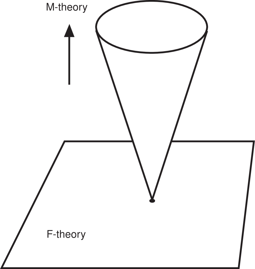
Figure 1: Picture of the branch structure. The cone represents the $3d$ Coulomb branch, where one resolves the singularities of the Calabi-Yau four-fold. The plane represents a ‘non-abelian’ $F$-theory branch where wrapped $M2$-branes have condensed, eg. a branch with a non-zero Fayet-Iliopoulos parameter. This branch is visible in the Higgs bundle description but not in the Calabi-Yau four-fold description. The picture is schematic in several respects, for example it is not guaranteed that every $F$-theory branch is connected to an $M$-theory branch.

We can further sharpen the claim that the $11d$ supergravity approach is not giving the full picture of singular $F$-theory compactifications. Recall that in this approach, one compactifies on an extra circle to three dimensions. The four-dimensional vector multiplet gains a pseudo-scalar upon compactification. Moving out on the $3d$ Coulomb branch makes the non-abelian gauge bosons very massive. In the dual $M$-theory picture, this scalar corresponds a Kähler modulus $\delta J=t_{X}\omega^{X}$ where $\omega^{X}$ is the $(1,1)$ form yielding a $U(1)_{X}$ gauge symmetry, $\delta C_{3}=A_{X}\wedge\omega^{X}$. Moving out on the Coulomb branch corresponds to making a small resolution, and taking the size of the exceptional cycles to be large, see figure 1. In the $M$-theory picture, an $M2$-brane wrapped on a cycle $\alpha$ has a mass proportional to

$$\int_{\alpha}J\ \sim\ q_{\alpha}^{X}\,t_{X},$$ (2.80)

where $q_{\alpha}^{X}=\int_{\alpha}\omega^{X}$ is its $U(1)_{X}$ charge, so in this limit, we can quantize $M2$-branes wrapped on the exceptional cycles.

Now we have seen that non-trivial configurations for $C_{3}$, such as arising from gluing VEVs or non-trivial bundles on non-reduced components of the spectral cover, can lift vector multiplets, and therefore part or all of the $3d$ Coulomb branch can get lifted. In particular, if a $U(1)_{X}$ gauge symmetry gets lifted by $C_{3}$ (eg. when the Fayet-Iliopoulos term is non-zero) then $t_{X}$ is frozen at zero and there are cycles which cannot get resolved. That is, the background value of the three-form field ${\sf C}_{3}$ can obstruct the small resolution, and the soliton quantization approach is not applicable to these interesting configurations, which as we shall see in part II give rise to all kinds of interesting flavour structures. This is analogous to the question of whether one can go through a conifold transition: it does not depend only on the geometry but also on the background fields, as they may lift the light fields whose VEV controls the transition.

2.7. Spectra of degenerate Higgs bundles

Now we would like to understand how to compute the spectra. As mentioned previously, these correspond to the infinitesimal deformations and are computed by the hypercohomology groups $\mathbb{H}^{p}({\cal E}^{\,\bullet})$ of the Higgs bundle. On the other hand, the most concrete way of constructing Higgs bundles is through the spectral data, so it would be most convenient to compute directly with this data. The hypercohomology groups can be directly computed in terms of the spectral data:

$$\mathbb{H}^{p}({\cal E}^{\,\bullet})\ =\ {\rm Ext}^{p}({\cal L},{\cal L})$$ (2.81)

Similarly we can compute the holomorphic couplings using Yoneda pairings. The $D$-terms are discussed in section LABEL:Dterms.

The basic strategy for the computation of any ${\rm Ext}$ group is to perform some kind of ‘resolution,’ i.e. relate ${\cal L}$ to some simpler sheaves, and then consider an associated long exact sequence. We can intuitively understand this as expressing a brane as a bound state, obtained by gluing simpler constituents together. Let us see how this works for degenerate cases.

The sheaf ${\cal L}$ decomposes into several pieces, and we are actually usually interested in computing ${\rm Ext}$-groups of the form

$${\rm Ext}_{X}^{p}(E,{\cal L})$$ (2.82)

where $X$ is our Calabi-Yau three-fold. To do this, let us suppose we can express ${\cal L}$ as an extension:

$$0\ \to\ B\ \to\ {\cal L}\ \to\ A\ \to\ 0$$ (2.83)

To compute ${\rm Ext}_{X}^{1}(E,{\cal L})$ and ${\rm Ext}_{X}^{1}({\cal L},E)={\rm Ext}_{X}^{2}(E,{\cal L})^{*}$, we use the associated long exact sequence:

$$\begin{array}[]{ccccccccc}0&\to&{\rm Ext}^{1}(E,B)&\to&{\rm Ext}^{1}(E,{\cal L})&\to&{\rm Ext}^{1}(E,A)&&\\[8.53581pt] &\to&{\rm Ext}^{2}(E,B)&\to&{\rm Ext}^{2}(E,{\cal L})&\to&{\rm Ext}^{2}(E,A)&\to&0\end{array}$$ (2.84)

In normal situations, the ${\rm Ext}^{0}$’s and ${\rm Ext}^{3}$’s all vanish, which we have assumed above to simplify the long exact sequence. This is not a limitation. If it is not satisfied, the story is much the same as below, except some additional generators may get lifted through the Higgs mechanism (which lifts ${\rm Ext}^{0}$ and ${\rm Ext}^{1}$ generators in pairs). But let us assume this is not needed here. Then we find that ${\rm Ext}^{1}(E,{\cal L})$ is generated by ${\rm Ext}^{1}(E,A\oplus B)$, except that some generators of ${\rm Ext}^{1}(E,A)$ may get killed by the coboundary map.

The mathematics of the long exact sequence can be expressed in terms of the effective Lagrangian of the brane system. In the brane bound state picture, we have deformations involving the constituent branes $A$ and $B$, i.e. we have chiral fields

$$X_{1}\in{\rm Ext}^{1}(E,B),\quad X_{2}\in{\rm Ext}^{1}(B,E),\quad Y_{1}\in{\rm Ext}^{1}(E,A),\quad Y_{2}\in{\rm Ext}^{1}(A,E)$$ (2.85)

Now all the $X_{p},Y_{p}$ may in principle descend to generators in ${\rm Ext}^{p}(E,{\cal L})$. However, some $Y_{1},X_{2}$ pairs may be lifted by interactions. In fact the coboundary map is simply the Yoneda pairing

$${\rm Ext}^{1}(E,A)\times{\rm Ext}^{1}(A,B)\ \to\ {\rm Ext}^{2}(E,B)$$ (2.86)

In other words, there are Yukawa couplings for the chiral fields

$$W\ \simeq\ Y_{1}\,F_{glue}\,X_{2}$$ (2.87)

where $F_{glue}\in{\rm Ext}^{1}(A,B)$ is the extension class. So when the gluing morphism $F_{glue}$ gets a VEV and we form the bound state ${\cal L}$, we see that the $X_{1}$ and $Y_{2}$ fields may pair up and get a mass through their Yukawa couplings to $F_{glue}$. This is how the lifting through the coboundary map translates to the effective Lagrangian. The surviving chiral fields correspond to the deformations in ${\rm Ext}^{1}(E,{\cal L})$ that we are after.

Note also that this is consistent with the charges under the extra $U(1)$ symmetry that appears as the gluing map is turned off. Up to an overall normalization, these charges are given by

$$Q(X_{1})=-Q(X_{2})=-Q(Y_{1})=Q(Y_{2})=+1,\qquad Q(F_{glue})=+2$$ (2.88)

In particular, the above Yukawa coupling is the only one allowed by the symmetries.

If $E={\cal L}$, then we can also resolve $E$ using a short exact sequence, and get a second long exact sequence involving the first argument of ${\rm Ext}$. Although the algebra gets more involved, it is in principle straightforward.

Let us apply this to the degenerate configurations in this paper. Consider first an intersecting configuration ${\cal L}$, with a non-zero gluing VEV. The support of ${\cal L}$ consists of two divisors $D_{1}$ and $D_{2}$, but the configuration should really be thought of as a single brane, as only the center-of-mass $U(1)$ gauge symmetry is unbroken. Let us denote by $i_{1}$ the inclusion $D_{1}\hookrightarrow X$, and similarly for $D_{2}$. Since the support is reducible, we have natural restriction maps to each component. Now suppose that the restriction $i_{1}^{*}{\cal L}\ =\ L_{1}$ is actually a line bundle. Then we can express ${\cal L}$ as an extension on $X$:

$$0\ \to\ i_{2*}L_{2}(-\Sigma)\ \to\ {\cal L}\ \to\ i_{1*}L_{1}\ \to\ 0$$ (2.89)

The second map is restriction to $D_{1}$ and then pushing forward to $X$. This is of the form (2.83), so we can apply the discussion above. The extension class is given by a holomorphic map in ${\rm Hom}_{\Sigma}(L_{1},L_{2})$. Similarly if the restriction to $D_{2}$ yields a line bundle, then we get an analogous extension sequence with $1$ and $2$ reversed.

Now in general the restriction to $D_{1}$ does not yield a line bundle, but a sheaf with torsion. We only know that there is a birational isomorphism between $L_{1}|_{\Sigma}$ and $L_{2}|_{\Sigma}$. Instead of working with a meromorphic map, an equivalent way to say this is there is another line bundle $L_{\Sigma}$ on $\Sigma$, and a pair of holomorphic maps in ${\rm Hom}_{\Sigma}(L_{1}|_{\Sigma},L_{\Sigma})$ and ${\rm Hom}_{\Sigma}(L_{2}|_{\Sigma},L_{\Sigma})$. Then we have the short exact sequence

$$0\ \to\ {\cal L}\ \to\ i_{1*}L_{1}\oplus i_{2*}L_{2}\ \to\ i_{\Sigma*}L_{\Sigma}\ \to\ 0$$ (2.90)

In other words, ${\cal L}$ is what might be called a Hecke transform of $i_{1*}L_{1}\oplus i_{2*}L_{2}$ along $\Sigma$. In this case we need the full long exact sequence for ${\rm Ext}$, not just the truncated version (2.84), but the advantage is that it applies generally.

Let us briefly check that (2.89) is indeed a special case of (2.90). Then we assume that the map ${\cal L}\to i_{1*}L_{1}$ is onto. The sheaf ${\cal L}$ is locally generated by sections $(s_{1},s_{2})$ such that $f_{1}s_{1}+f_{2}s_{2}=0$ on the intersection. Now let us ask for the kernel of the map ${\cal L}\to i_{1*}L_{1}$. It is generated by sections $s_{2}$ such that $f_{2}s_{2}|_{\Sigma}=0$, i.e. $s_{2}|_{\Sigma}=0$ assuming $f_{2}$ does not vanish identically. But this is the definition of $i_{2*}L_{2}(-\Sigma)$.

Similarly we may consider the case that ${\cal L}$ consist of a line bundle over a non-reduced surface. For the simplest case where the Higgs field is a Jordan block of rank two, we found the extension sequence

$$0\ \to\ i_{*}(L(\Sigma)\otimes K^{-1})\ \mathop{\to}^{i}\ {\cal L}\ \mathop{\to}^{r}\ i_{*}L\ \to\ 0$$ (2.91)

When there are Jordan blocks of higher rank, as discussed we can iterate this. This is again of the form (2.83), so we temporarily replace ${\cal L}$ by $A\oplus B$, where $A=i_{*}L$ and $B=i_{*}(L(\Sigma)\otimes K^{-1})$, and then lift pairs of deformations by turning on the extension class in the long exact sequence.

In cases where we are already given some explicit representative of the non-abelian holomorphic bundle $E$ and the Higgs field $\Phi$, we can use the short exact sequence (2.6) to find ${\cal L}$ and then compute ${\rm Ext}$ groups. Probably it is then simplest to use computer algebra.

2.8. Chiral matter and the index

In the previous subsection we explained the tools to compute the matter content of the theory. The calculations are in principle straightforward, and can even be carried out by computer algebra systems like Macaulay2. However in order to get a quick overview of a model, it is often sufficient to know only the net amount of chiral matter. This can be computed much more efficiently using the index theorem:

$$\chi(F,G)\ =\ \sum_{i=1}^{3}(-1)^{i}\,{\rm Ext}^{i}(F,G)\ =\ \int_{X}{\bf ch}(F^{\vee}){\bf ch}(G)\hat{\bf A}(TX)$$ (2.92)

For the cases of interest, it is often true that ${\rm Ext}^{0}$ and ${\rm Ext}^{3}$ vanish (no ghosts), and so $\chi$ reduces to the net amount of chiral matter. These formulae make sense for the reducible and non-reduced cases we are interested in. It applies when $F$ and $G$ are merely coherent sheaves (or even complexes thereof), and $X$ is projective (see eg. [35, 36]).

In the IIb context this formula can be understood from anomaly inflow. In the $F$-theory context, the ‘charge vector’ ${\bf ch}(F){\bf A}(TX)^{1/2}\in H^{even}(X)$ is not defined on the IIb space-time, but on the auxiliary Calabi-Yau three-fold $X$. In this context we actually only need part of the charge vector; it can be related to the couplings of the NS two-form under $F$-theory/heterotic duality, and is therefore again closely tied to anomalies.

To find the Chern classes of more complicated sheaves, we can use one of the fundamental properties of the Chern character. If we have a short exact sequence

$$0\ \to\ M^{\prime}\ \to\ M\ \to\ M^{\prime\prime}\ \to\ 0$$ (2.93)

then

$${\bf ch}(M)\ =\ {\bf ch}(M^{\prime})+{\bf ch}(M^{\prime\prime})$$ (2.94)

The index formula also involves the dual, $F^{\vee}$. In good situations, the dual is again a sheaf, for instance for a line bundle on a smooth divisor in $X$ we have $(i_{*}L)^{\vee}=i_{*}(L^{\vee}\otimes K_{D})$. More generally, it is not possible to require that the dual is another sheaf while preserving all the expected properties, and the dual is instead given by a complex, $F^{\vee}=RHom^{\bullet}(F,K_{X})$ [35]. Fortunately for our purposes we only need the following property:

$${\rm ch}_{i}(F^{\vee})\ =\ (-1)^{i}{\rm ch}_{i}(F)$$ (2.95)

Let us apply this to the cases considered in this paper. For a vector bundle $L$ supported on a smooth divisor $D$ we have

$$\begin{array}[]{cclcccl}{\rm ch}_{0}(i_{*}L)&=&0&&{\rm ch}_{2}(i_{*}L)&=&i_{*}c_{1}(\hat{L})\\ {\rm ch}_{1}(i_{*}L)&=&{\rm rk}(L)\,D&&{\rm ch}_{3}(i_{*}L)&=&i_{*}\left({\rm ch}_{2}(\hat{L})+{1\over 24}{\rm rk}(L)c_{1}(K_{D})^{2}\right)\end{array}$$ (2.96)

where $\hat{L}=L\otimes K_{D}^{-1/2}$. The twisting by $c_{1}(K_{D})$ is familiar from the Freed-Witten anomaly, which says that the gauge field really takes values in the bundle $L\otimes K_{D}^{-1/2}$ on $D$, and so the flux is given by

$${{\rm Tr}(F)\over 2\pi}\ =\ c_{1}(\hat{L})\ =\ c_{1}(L)-\frac{1}{2}\,{\rm rk}(L)\,c_{1}(K_{D})$$ (2.97)

Using the above, it is very simple to reproduce the standard formula for the net amount of matter localized on brane intersections or in the bulk of a 7-brane, assuming no gluing morphisms are turned on. But we can equally well do the degenerate configurations. For the reducible case, we used the short exact sequence

$$0\ \to\ i_{2*}L_{2}(-\Sigma)\ \to\ {\cal L}_{1}\ \to\ i_{1*}L_{1}\ \to\ 0$$ (2.98)

Therefore we find

$$\begin{array}[]{rcl}{\rm ch}_{0}({\cal L}_{1})&=&0\\ {\rm ch}_{1}({\cal L}_{1})&=&D_{1}+D_{2}\\ {\rm ch}_{2}({\cal L}_{1})&=&i_{1*}c_{1}(\hat{L}_{1})+i_{2*}c_{1}(\hat{L}_{2})-i_{\Sigma*}\Sigma\end{array}$$ (2.99)

Similarly, in the non-reduced case we had the sequence

$$0\ \to\ i_{*}(L(\Sigma)\otimes K_{D}^{-1})\ \mathop{\to}^{i}\ {\cal L}\ \mathop{\to}^{r}\ i_{*}L\ \to\ 0$$ (2.100)

and from this we find

$$\begin{array}[]{rcl}{\rm ch}_{0}({\cal L}_{2})&=&0\\ {\rm ch}_{1}({\cal L}_{2})&=&2D\\ {\rm ch}_{2}({\cal L}_{2})&=&2\,i_{*}c_{1}(\hat{L})-i_{*}c_{1}(K_{D})+i_{\Sigma*}\Sigma\end{array}$$ (2.101)

As a simple example, let us consider the reducible brane ${\cal L}_{1}$, and intersect it with another brane $i_{3*}L_{3}$. We find

$$\chi({\cal L}_{1},i_{3*}L_{3})\ =\ \int_{D_{1}\cdot D_{3}}\left[c_{1}(\hat{L}_{1})-c_{1}(\hat{L}_{3})\right]+\int_{D_{2}\cdot D_{3}}\left[c_{1}(\hat{L}_{2}(-\Sigma))-c_{1}(\hat{L}_{3})\right]$$ (2.102)

This is the conventional formula when we turn off the gluing VEV. Indeed the index should not change under such a continuous deformation. It should be remembered however that when the gluing morphism has both poles and zeroes, then it cannot be turned off holomorphically, and we have to use (2.90) instead.

Similarly, let us consider the intersection of the non-reduced brane ${\cal L}_{2}$ with $i_{3*}L_{3}$. Then we have

$$\chi({\cal L}_{2},i_{3*}L_{3})\ =\ \int_{D\cdot D_{3}}\left[c_{1}(\hat{L})-c_{1}(\hat{L}_{3})\right]+\left[c_{1}(\hat{L}(\Sigma))-c_{1}(K_{D})-c_{1}(\hat{L}_{3})\right]$$ (2.103)

as we would when the gluing data is turned off.

2.9. Boundary CFT description

We have described non-reduced schemes as configurations in supersymmetric Yang-Mills theory. In the type II context, one naturally asks if there is also a boundary CFT description. The first thing to try is a free-field description. Normally we would have

$$\partial_{1}X(\sigma)|_{0}\ =\ 0$$ (2.104)

and then we tensor with Chan-Paton indices. For non-reduced configurations we want instead

$$\partial_{1}X^{2}(\sigma)|_{0}\ =\ 2X\partial_{1}X|_{0}\ =\ 0$$ (2.105)

and further we want $\partial_{1}X(\sigma)|_{0}\not=0$, for otherwise we reduce to the previous case. This is a non-linear condition on the mode expansion. In some sense this indicates we are dealing with true non-abelian configurations. Therefore it does not seem likely that we can find a free-field description.

There are however other methods for constructing boundary CFTs. One such description is the boundary linear sigma model [37, 38, 39]. It can be developed largely in parallel with $(0,2)$ linear sigma models, which we briefly review in section 4.3 of part II.

We will keep things extremely simple and only explain the main idea. Apart from the $(2,2)$ chiral fields $X_{i}$ and vector multiplet in the bulk, we consider boundary chiral fields $P$ and boundary Fermi fields $\Lambda_{a},\Gamma$. We have a boundary superpotential

$$\int dx^{0}\,d\theta\ \Gamma\,S(X_{i})+\Lambda_{a}PJ^{a}(X_{i})|_{\bar{\theta}=0}+h.c.$$ (2.106)

The $\Lambda_{a}$ lead to Chan-Paton factors, and $\Gamma$ is designed to pair up with bulk fermions normal to $S(x_{i})=0$. In the large volume regime, the massless modes of $\Lambda_{a}$ live in a bundle $\tilde{V}$ on $X$ defined by a short exact sequence

$$0\ \to\ \tilde{V}\ \to\ \bigoplus_{a}{\cal O}(q_{a})\ \mathop{\longrightarrow}^{J^{a}}\ {\cal O}(q_{0})\ \to\ 0$$ (2.107)

The effect of the first term of the boundary superpotential is then to restrict the open string ends to $S(x)=0$, so that we end up with $V=\tilde{V}|_{S=0}$. This basic construction can be extended in several directions.

This allows us to construct CFT descriptions of non-reduced configurations. For instance the structure sheaf ${\cal O}_{2D}$ of a non-reduced scheme $2D$ fits into the exact sequence

$$0\ \to\ {\cal O}_{X}(-2D)\ \to\ {\cal O}_{X}\ \to\ {\cal O}_{2D}\ \to\ 0$$ (2.108)

Taking the dual, this naturally fits in the boundary LSM description above. Similarly, one can construct the structure sheaf ${\cal O}_{D}$ of a reducible divisor, by taking a section of ${\cal O}_{X}(D)$ which is factorizable. This configuration has a non-zero gluing VEV along the intersection of the irreducible pieces. We expect that the linear sigma model flows to a CFT only when the configuration is (Gieseker) poly-stable.

3. The D-terms

3.1. The hermitian-Einstein metric and stability

In previous sections, we studied the $F$-terms of the $8d$ gauge theory. $F$-flatness is preserved under complexified gauge transformations. Modulo such complexified gauge transformations, the only invariant data in the $F$-terms is the spectral data. We used this extensively for writing down solutions for the $F$-term equations, by writing down the spectral sheaf.

The $D$-terms for the $8d$ gauge theory compactified on a Kähler surface $S$ are given by the following ‘hermitian-Einstein’ equation:

$$g^{i\bar{j}}F_{i\bar{j}}+[\Phi^{2,0\dagger},\Phi^{2,0}]\ =\ -\sqrt{-1}\,\zeta I$$ (3.1)

with $\zeta\simeq{\rm deg}(E)/(r\,{\rm vol}(S))$. Here we think of the commutator as a $(0,0)$-form by contracting with the volume form of $S$. Unlike the $F$-terms, the $D$-terms are not invariant under the complexified gauge transformations. They require us to choose a hermitian metric, or equivalently a reduction of the complexified structure group to a compact subgroup.

It may be useful to briefly recall some aspects of connections on holomorphic vector bundles [40]. A frame for $E$ over an open subset $U$ is a collection of sections $H=\{e_{1},..,e_{r}\}$ forming a basis for each fiber over $U$. With a suitable choice of coordinates on the fiber, we can write the hermitian metric in matrix notation as

$$h\ =\ HH^{\dagger}$$ (3.2)

where $H$ is a map from $S$ to $GL(n,{\bf C})/U(n)$. The frame is said to be unitary if $h_{a\bar{b}}=\delta_{a\bar{b}}$. The frame is said to be holomorphic if the $e_{a}$ are holomorphic maps from $U$ to $E$.

If the structure group is to be $U(n)$ rather than $GL(n,{\bf C})$, then the gauge covariant derivative must respect the hermitian metric. In the unitary frame, this implies that $A^{+}=-A$, where the superscript denotes transpose and complex conjugation. In a more general frame however, this implies that $A^{\dagger}=-h^{-1}A^{+}h$, i.e. the adjoint depends on the hermitian metric. Similarly the adjoint $\Phi^{\dagger}$ corresponds to $h^{-1}\Phi^{+}h$.

We can further fix the connection by requiring the connection to be compatible with the complex structure, i.e. the $(0,1)$ part of the covariant derivative is given by $\bar{\partial}$ (so $A^{0,1}=0$ in a holomorphic frame). In such a frame, the zero modes and superpotential are independent of the Kähler moduli, and computations reduce to questions in complex geometry and algebraic geometry. With this additional condition, we find that the connection is uniquely determined as

$$A^{1,0}\ =\ -(\partial h)h^{-1}$$ (3.3)

in the holomorphic frame. This connection is sometimes referred to as the Chern connection. We can switch back to a unitary frame by performing a complex gauge transformation by $H$. In this unitary frame the connections are given by

$$H^{-1}(\partial+A^{1,0})H\ =\ \partial-(\partial H^{\dagger})H^{\dagger\,-1},\qquad H^{-1}\bar{\partial}H\ =\ \bar{\partial}+H^{-1}(\bar{\partial}H)$$ (3.4)

Thus assuming we have fixed the $F$-term data, we see that the $D$-terms may be viewed as the following equation for the hermitian metric $h$ on $E$:

$$g^{i\bar{j}}\partial_{\bar{j}}(\partial_{i}h\,h^{-1})+[h^{-1}\Phi^{+}h,\Phi]-\sqrt{-1}\,\zeta I\ =\ 0$$ (3.5)

The solution is usually called the hermitian-Einstein metric. To distinguish it from the hermitian metric which arises as a special case when $\Phi=0$, we might also call it the hermitian Yang-Mills-Higgs metric, but this terminology is perhaps too lengthy.

The solution to the abelian part of this equation can be found by making a conformal change in the metric, $h\to he^{f}$ and solving for $f$. The non-abelian equations are much harder to solve. We could solve the $F$-terms by writing down suitable spectral data. However this approach does not work for the $D$-terms, even in the generic case where the eigenvalues are mutually distinct over an open subset, and thus we can diagonalize by a complex gauge transformation. The problem is that if $\Phi$ commutes with its adjoint in one frame, then it will generally not commute with its adjoint in another frame that is related by a complexified gauge transformation. But the frame depends on the choice of hermitian metric, which must be solved for.

Fortunately, the existence of a solution to the non-abelian part of the $D$-terms can still be phrased in algebro-geometric terms, through a Higgs bundle analogue of the Uhlenbeck-Yau theorem. Let us make some definitions. A subbundle $F\subset E$ is said to be a Higgs subbundle if $\Phi(F)\subset F\otimes K$. A Higgs bundle is said to be $J$-stable if

$$\mu(F)<\mu(E)$$ (3.6)

for every Higgs subbundle, where the slope is defined as usual, $\mu=J$-degree/rank. A Higgs bundle is semi-stable if $\mu(F)\leq\mu(E)$ for every Higgs subbundle. Finally, a Higgs bundle is poly-stable if it is a direct sum of stable Higgs bundles with the same slope. Then the general principle is that the algebro-geometric criterion of poly-stability should be equivalent to the differential geometric criterion of the existence and uniqueness of the hermitian-Einstein metric. (For abelian bundles, this requires adding the explicit Fayet-Iliopoulos term $\zeta$ to the equation).

The condition of stability as a bundle is clearly stronger than the condition of stability as a Higgs bundle. A Higgs bundle is stable if the underlying bundle is. But a bundle which is blatantly unstable can still be stable as a Higgs bundle. As a well-known example, consider a Riemann surface $\Sigma_{g}$ with $g\geq 2$ and choose a square root $K^{1/2}$ of the canonical bundle. Then take

$$E\ =\ K^{-1/2}\oplus K^{1/2},\qquad\Phi\ =\ \left(\begin{array}[]{cc}0&1\\ 0&0\\ \end{array}\right)$$ (3.7)

Then $E$ is unstable as a bundle, but stable as a Higgs bundle. The slope of $E$ vanishes, and the slope of the Higgs sub-bundle $K^{-1/2}$ is negative. The sub-bundle $K^{1/2}$, which destabilizes $E$, is not preserved by the Higgs field.

Higgs bundles with generic spectral covers are stable. If the spectral cover is smooth and irreducible, then the Higgs bundle does not have any Higgs sub-bundles. In the next subsection we would like to discuss stability when the spectral cover is not smooth and irreducible.

Now we would like to compare this with the ALE fibration picture. The cylinder mapping is a construction in algebraic geometry, so the $F$-term data in the Higgs bundle description, the spectral cover description and in the ALE fibration can be mapped exactly. On the other hand, the hermitian-Einstein metric $h$ will not be diagonal and the gauge field $A\sim h^{-1}\partial h$ will be non-abelian. This means that the $W$-bosons (i.e. the off-diagonal components of the gauge field) will be condensed. On the other hand, in the ‘closed string’ ALE fibration picture the $W$-bosons are extended solitons and do not have an off-shell description. This means that a true ten/twelve dimensional solution does not exist on the type II side, except perhaps in some fuzzy sense, as the light $W$-bosons are not properly incorporated in the effective action when the elliptic Calabi-Yau four-fold develops singularities and cannot be condensed in this description. In the Higgs bundle description the non-abelian degrees of freedom are included, and this is why the Higgs bundle ‘resolves’ the singularities of the Calabi-Yau fourfold and provides a smooth weakly coupled description.

This is a general phenomenon in heterotic/type II duality. The very same phenomenon, in six dimensions instead of in eight dimensions, was previously encountered very explicitly in [12]. There we studied gravitationally dressed versions of ’t Hooft-Polyakov monopole solutions in type IIa on $K3$. Such monopoles satisfy Bogomol’nyi equations, a close cousin of Hitchin’s equations. As described in [12], the abelian part of this solution (a Dirac monopole) is singular but can be lifted to ten dimensions, where one encounters a $K3$ with $A_{1}$ singularity. To ‘resolve’ the singularities, we incorporated non-abelian gauge fields in the effective action. Then the non-abelian part of the resulting solution smoothed out the singularities of the abelian solution through exponentially small corrections. But these corrections came from condensation of extended solitons in $10d$. Such degrees of freedom cannot be described by a local Lagrangian in $10d$, and thus the full non-abelian solution could not be lifted. We encounter the same problem here. One can try to integrate out the $W$-bosons and write an abelian solution, which is singular at the branch locus of the spectral cover. To smooth out the singularities however, we need to include non-perturbative gauge fields, as in [12].

As we noted in the introduction, this means that global models will have difficulty capturing some non-abelian aspects of the local model. In particular, in order to write down physical wave functions and compute the Kähler potential in an approximation we can trust, we need the hermitian-Einstein metric, which is not an object in algebraic geometry and exists only in the Higgs bundle picture.

The question then arises if there isn’t another way to deal with the $D$-terms if we were working in the ALE fibration picture. Here we can go back to the analogue of Uhlenbeck-Yau for Higgs bundles. The criterion of existence and uniqueness of the hermitian-Einstein metric can be phrased in terms of slope-stability. This is an algebro-geometric concept which we could try to compare in the Higgs bundle, spectral cover, and Calabi-Yau four-fold pictures. As we discuss in more detail in the next section, slope-stability can be defined in terms of Fayet-Iliopoulos parameters. According to [41, 1], the Fayet-Iliopoulos parameters in $F$-theory are given by $\zeta_{X}\simeq m_{10}^{4}\int G\wedge J\wedge\omega_{X}$. The difficult parts are (1) to properly define all possible configurations of $C_{3}$ on a singular Calabi-Yau in mathematical way, including the non-obvious configurations considered in this paper, and (2) to define an analogue of the notion of a sub and a quotient. This requires us to generalize the notion of ${\rm Ext}^{0}$ for sheaves to ALE fibrations. These notions are currently not available, but it is clear that some analogue should exist at least in the context of ALE or del Pezzo fibrations, because the map between spectral covers and ALE fibrations is an algebraic one, so we can in principle define them by mapping to the spectral cover side.

At any rate, given the relation with Higgs bundles it appears inevitable that the primitiveness condition $J\wedge G=0$ must be replaced by some notion of slope-stability for Calabi-Yau four-folds with $G$-flux. Although in general we cannot write the physical wave functions in the Calabi-Yau four-fold or spectral cover pictures, if phrased in such terms, the essential information of existence and uniqueness of the hermitian-Einstein metric can be preserved. This is an important qualitative change, because primitiveness is a closed condition, whereas stability is an open condition and leads to a chamber structure in the Kähler moduli space.

We emphasize again that this situation is not unique to $F$-theory. For example in the context of $M$-theory on $G_{2}$-manifolds, the $G_{2}$-metric is singular near the three-cycle where the gauge theory is localized and is therefore not the correct metric for physics purposes. To understand the physics near such three-cycles, we need some way to ‘resolve’ the singularities and obtain a smooth weakly coupled description. This was achieved only recently in [20], by replacing the singular $G_{2}$ metric by the harmonic metric on a Higgs bundle. The harmonic metric is smooth and includes non-abelian corrections, but again only exists in the Higgs bundle picture. Thus even when new techniques for constructing compact $G_{2}$-holonomy manifolds become available, in the regime of interest the $G_{2}$-metric can’t be trusted and we still have to go back to the local model in order to study the $D$-terms (using the harmonic metric).

3.2. Stability for degenerate cases

In the previous subsection we rephrased the existence and uniqueness of the hermitian-Einstein metric in terms of slope-stability of the Higgs bundle. Because Higgs bundles are usually constructed by writing down spectral data, it would be more convenient to have a stability criterion for the spectral sheaf. However we have seen that the spectral data for a smooth Higgs bundle can easily have singular behaviour, for example the spectral cover can be reducible or non-reduced. Thus we need a criterion that behaves well under degenerations, and remains equivalent to existence and uniqueness of the hermitian-Einstein metric in the Higgs bundle picture even in such degenerate cases.

The theory of stable sheaves is generally credited to Gieseker, Maruyama, and Simpson [42], and is based on the Hilbert polynomial. The Hilbert polynomial is defined purely algebraically and is constant in flat families, even if some members of the family are degenerate. Physically speaking this implies for instance that the net number of generations cannot jump.

Thus instead of a Kähler class $J$, we consider an ample line bundle ${\cal O}(1)$ whose first Chern class is proportional to $J$. Then we consider the associated Hilbert polynomial

$$P_{\rm Hilb}({\cal L},m)\ =\ \chi({\cal L}\otimes{\cal O}(m))$$ (3.8)

where of course $\chi(F)=\sum(-1)^{i}{\rm Ext}^{i}({\cal O}_{X},F)$. We define the coefficients

$$P_{\rm Hilb}({\cal L},m)\ =\ \sum_{k=0}^{d}p_{k}({\cal L}){m^{k}\over k!}$$ (3.9)

Using Riemann-Roch, they can be expressed in terms of Chern classes. The degree of $P_{\rm Hilb}({\cal L},m)$ is the dimension of the support of ${\cal L}$, and the coefficient $p_{i}$ of the leading term is called the rank. In our case, we will be interested in sheaves that are supported in dimension two on a three-fold, so $p_{3}=0$ and $d=3$. Then, the slope is defined as

$$\mu({\cal L})\ =\ {p_{1}({\cal L})\over p_{2}({\cal L})}$$ (3.10)

and slope-stability is defined in the usual way. Note that this makes sense for arbitrary coherent sheaves on a projective variety, in particular reducible or non-reduced cases. (There is also the notion of Gieseker stability, which uses the normalized Hilbert polynomial $p({\cal L},m)=P({\cal L},m)/{\rm rank}$ instead of the slope, but we do not know how to justify this in the context of $F$-theory).

To apply this to our case, we let $\bar{X}$ be the projective closure of $X$. We may pick an ample ${\cal O}(1)_{\bar{X}}$ which restricts to ${\cal O}(1)$ on $X$. Then, provided the spectral cover does not intersect infinity, slope-stability for the spectral sheaf is the same as slope-stability for the Higgs bundle. To see this, Kähler classes on $\bar{X}$ are of the form

$$\pi^{*}J_{B}+tJ_{0}$$ (3.11)

where $J_{B}$ is a class on the base, $J_{0}$ is the Poincaré dual of the zero section, and $t$ is a real number. Restricting to $X$, the class $J_{0}$ trivializes, and we are left with $\pi^{*}J_{B}$. Then stability of ${\cal L}$ with respect to $\pi^{*}J_{B}$ is the same as stability of $E=p_{C*}{\cal L}$ with respect to $J_{B}$ (or any multiple of it), because $H^{i}(C,{\cal L}\otimes(p_{C}^{*}L)^{m})\cong H^{i}(S,E\otimes L^{m})$. But $\pi^{*}J_{B}$ is not a Kähler class on $\bar{X}$. To fix this, we consider a small perturbation by $\epsilon J_{0}$. Since stability is an open condition, a sufficiently small perturbation preserves stability. Then by rescaling $J_{B}+\epsilon J_{0}$ and relabelling $J_{B}$, we see that stability of ${\cal L}$ agrees with stability for the Higgs bundle. Slope-stability is also usually preserved under the Fourier-Mukai transform, for instance in the context of heterotic spectral covers [43].

We can also adapt these statements when there is a parabolic structure. One may define a slope for parabolic sheaves, and use this to define stability for the spectral sheaf.

Thus stability for sheaves gives a practical way to see if the $D$-terms are satisfied. In particular this gives a simple way to derive a statement in the previous subsection: generic Higgs bundles, for which the spectral sheaf is actually an honest line bundle, are stable. This follows simply because any line bundle is stable.

From Riemann-Roch we get

$$p_{2}\ =\ {\rm ch}_{1}({\cal L})J^{2},\qquad p_{1}\ =\ {\rm ch}_{2}({\cal L})J+{\rm ch}_{0}({\cal L}){c_{2}(TX)\over 12}J$$ (3.12)

For the special case of a bundle $L$ on a divisor $D$, ${\cal L}=i_{*}L$, we have ${\rm ch}_{0}=0$, ${\rm ch}_{1}={\rm rank}(L)\,D$, and ${\rm ch}_{2}=i_{D*}c_{1}(\hat{L})$, leading to

$$p_{2}\ =\ {\rm rank}(L)\int_{D}J\wedge J,\qquad p_{1}\ =\ \int_{D}J\wedge c_{1}(\hat{L})$$ (3.13)

where $\hat{L}=L\otimes K_{D}^{-1/2}$, and so the expression for the slope reduces to the usual one.

The Chern characters for several configurations of interest were discussed in section LABEL:Index, and can easily be used to write down the slope. For instance for the reducible case, where ${\cal L}$ is given by an extension

$$0\ \to\ i_{2*}L_{2}(-\Sigma)\ \to\ {\cal L}\ \to\ i_{1*}L_{1}\ \to\ 0$$ (3.14)

the Chern character of ${\cal L}$ is given in equation (2.99), and therefore the slope is given by

$$\mu({\cal L})\ =\ {\deg(\hat{L}_{1})+\deg(\hat{L}_{2})-\int_{\Sigma}J\over{\rm vol}(D_{1})+{\rm vol}(D_{2})}$$ (3.15)

In this case, $i_{*}L_{2}(-\Sigma)$ is clearly a potential destabilizing subsheaf, whereas $i_{*}L_{1}$ is not a subsheaf.

In the effective theory, the slopes are closely related to field dependent Fayet-Iliopoulos terms. Let us consider for example a configuration of $7$-branes ${\cal L}$ in type IIb. We are interested in the reducible case, i.e. we have ${\cal L}=\oplus_{n}{\cal L}_{n}$ where the ${\cal L}_{n}$ are irreducible. The abelian generators of the low energy gauge group are given by ${\rm Ext}^{0}({\cal L}_{n},{\cal L}_{n})$ and the non-abelian generators are given by ${\rm Ext}^{0}({\cal L}_{m},{\cal L}_{n})$ with $n\not=m$. Suppose the low energy gauge group is $G$, and let $\xi:G\to U(1)$ be a character. At the level of the Lie algebra, it corresponds to a linear combination $\sum_{n}\xi_{n}\omega_{n}$ where $\omega_{n}$ is the generator of ${\rm Ext}^{0}({\cal L}_{n},{\cal L}_{n})$. To each such $\xi$ we associate a twisted version of the Chern character. Intuitively we think of this as the Chern character of a rank one sheaf ${\cal L}_{\xi}$ corresponding to the $U(1)$ gauge symmetry, although ${\cal L}_{\xi}$ may strictly not exist:

$${\bf ch}({\cal L}_{\xi})\ =\ \sum_{n}\xi_{n}\,{\bf ch}({\cal L}_{n})$$ (3.16)

Then for each $\xi$ we get a shift symmetry on the Kähler moduli space

$$\delta_{\lambda_{\xi}}\,{\rm Im}(T_{D})\ =\ [\omega^{(2)}({\cal L}_{\xi},\lambda_{\xi})]_{2}\cdot D\ \simeq\ \lambda_{\xi}\,{\rm ch}_{2}({\cal L}_{\xi})\cdot D$$ (3.17)

where $\omega^{(2)}({\cal L}_{\xi},\lambda_{\xi})$ is obtained by descent:

$${\bf ch}({\cal L}_{\xi}){\bf A}^{1/2}(X)\ =\ d\,\omega^{(1)}({\cal L}_{\xi}),\qquad\delta_{\lambda_{\xi}}\omega^{(1)}\ =\ d\,\omega^{(2)}({\cal L}_{\xi},\lambda_{\xi})$$ (3.18)

In general such a shift symmetry is deduced from the Chern-Simons couplings of the gauge fields to anti-symmetric tensor fields. In IIb this follows from the Chern-Simons coupling of ${\cal L}$ to $C^{(4)}_{RR}$. Although the expression was derived for smooth configurations, in this form it applies equally well to general coherent sheaves, like the reducible or non-reduced configurations considered in this paper, or even a complex of such. The reason is that we can resolve each ${\cal L}_{n}$ as a sequence of vector bundles. Since the Chern character is additive, we apply descent to the individual pieces, and then we add them back together with appropriate signs. In the heterotic setting, we get essentially the same story by considering the transformation law for $B^{(2)}_{NS}$ and $\tilde{B}^{(6)}_{NS}$, and in IIa we would consider the transformation law for $C^{(3)}_{RR}$.

Apart from an isometry, to define a moment map we further need a Kähler form on the moduli space. This is also determined by the string compactification. In the large volume limit, it can be determined by a Kaluza-Klein reduction, and in type IIb for example is given by the second derivative of the following Kähler potential:

$${\cal K}\ =\ -2M_{Pl}^{2}\log{\cal V}$$ (3.19)

where ${\cal V}$ is the volume as a function of the Kähler moduli. With this potential, the Fayet-Iliopoulos parameter (or moment map for the Killing vector field of the shift symmetry) is precisely given by the slope $\mu({\cal L}_{\xi})$, up to an over-all factor which is moduli dependent but independent of the details of the brane.

We would like to reexamine the mathematical notion of slope stability in light of this relation between the slope and the Fayet-Iliopoulos parameter in the effective Lagrangian. It helps to generalize slightly and consider an abstract brane $E$, which can be a bundle, a coherent sheaf, a Lagrangian submanifold or a boundary state depending on the context. In this article we have argued it must be even further extended to ALE fibrations. Then we have the following well-known and universal phenomenon in string compactification.

We adjust the Kähler moduli until $E$ becomes marginally stable to decay into two subobjects, $E^{\prime}$ and $E^{\prime\prime}$. Then one finds that at the locus of marginal stability, the effective theory is described by a version of the Fayet model [44, 45, 46, 47]. That is, first of all we get an extra $U(1)$ gauge symmetry $U(1)_{X}$, equivalently an extra generator

$$\Lambda_{X}\ \in\ {\rm Ext}^{0}(E,E)$$ (3.20)

This is practically the definition of marginal stability. At the wall of marginal stability, $E$ becomes semi-stable, and the solution of the $D$-terms yields the unique reducible object with the same graded sum, $E\sim E^{\prime}\oplus E^{\prime\prime}$. Then ${\rm Ext}^{0}(E,E)$ is at least two-dimensional, with $\Lambda^{\prime}\in{\rm Ext}^{0}(E^{\prime},E^{\prime})$ and $\Lambda^{\prime\prime}\in{\rm Ext}^{0}(E^{\prime\prime},E^{\prime\prime})$, and we identify $\Lambda_{X}=\Lambda^{\prime}-\Lambda^{\prime\prime}$. Secondly, we get an extra generator $X\in{\rm Ext}^{1}(E,E)$, i.e. a chiral field $X$ in ${\rm Ext}^{1}(E^{\prime},E^{\prime\prime})$ or ${\rm Ext}^{1}(E^{\prime\prime},E^{\prime})$. From the Yoneda pairing ${\rm Ext}^{0}\times{\rm Ext}^{1}\to{\rm Ext}^{1}$, we see that the chiral field is charged under $U(1)_{X}$, i.e. we have

$$\delta X\ =\ \Lambda^{\prime}X-X\Lambda^{\prime\prime}$$ (3.21)

When $X$ gets a VEV, we see that $X\sim X+\Lambda_{X}$, so $X$ becomes exact and $\Lambda_{X}=\Lambda^{\prime}-\Lambda^{\prime\prime}$ is no longer closed, and both are removed from the massless spectrum. Using the Hermitian metric to separate complexified gauge transformations in actual gauge transformations and $D$-terms, this is equivalent to saying that the $U(1)$ is Higgsed, and we have a $D$-term potential of the form

$$V_{D}\ =\ \frac{1}{2}(\zeta_{X}-q_{X}|X|^{2})^{2}$$ (3.22)

which is a version of the Fayet model.

Now let us connect this with the notion of slope stability. We regard $F$ as a non-trivial extension of $E^{\prime}\oplus E^{\prime\prime}$. Then the relevant $U(1)$ symmetry is $\rho_{\xi}=\Lambda^{\prime}-\Lambda^{\prime\prime}$, so we have

$$\zeta_{X}\ =\ \mu(E^{\prime})-\mu(E^{\prime\prime})$$ (3.23)

From the $D$-term potential of the Fayet model, when $\zeta_{X}>0$ we find that $X$ gets a VEV and we form a bound state. When $\zeta_{X}=0$ there is a supersymmetric vacuum with $\left\langle X\right\rangle=0$ and massless $U(1)_{X}$. And when $\zeta_{X}<0$, supersymmetry is broken by $D$-terms. Now it is not hard to prove that if $F$ is given by an extension

$$0\to E^{\prime\prime}\to F\to E^{\prime}\to 0$$ (3.24)

then we have either $\mu(E^{\prime\prime})<\mu(F)<\mu(E^{\prime})$ or $\mu(E^{\prime\prime})>\mu(F)>\mu(E^{\prime})$. Assuming there are no other light fields in the $D$-term potential, it follows that $F$ is stable for $\zeta_{X}>0$, $E^{\prime}\oplus E^{\prime\prime}$ is poly-stable for $\zeta_{X}=0$, and the system is unstable for $\zeta_{X}<0$. This seems to agree nicely with our discussion of slope stability.

However, there is an important subtlety in the above discussion, which seems to be ignored in the literature. What we really want to consider is infinitesimal deformations, i.e. deformations over the dual numbers $D={\bf C}[\varepsilon]/\varepsilon^{2}$ (see eg. [22]). Physically the reason for this is that the Fayet model is only an effective description for the linearized deformations. We could certainly also consider finite deformations, but stability is a highly non-linear condition and the Fayet model could hardly be expected to capture this. In fact for intersecting brane configurations, there are always at least two natural and inequivalent quotient branes, given by restricting to either of the two intersecting components. It is not hard to see that they give inequivalent restrictions on the slope. Therefore for a finite deformation we get at least two inequivalent ‘decay modes’ for which we have to test stability, whereas the Fayet model sees only one. Ignoring the second ‘decay mode’ quickly leads to contradictions with Murayama’s boundedness result. But it seems natural to conjecture that in generic enough situations, testing against these two decay modes should be sufficient to ensure stability for a finite deformation. This will be the de facto assumption in some of the examples in part II.

3.3. Numerical approach with balanced metrics

As usual in supersymmetric string compactification, the zero modes and superpotential can be determined up to field redefinitions by methods of algebraic geometry. As we discussed in detail, even the existence of a solution of the $D$-term equations can be characterized in algebro-geometric terms. However, for certain questions existence does not suffice, and we need to have an explicit knowledge of the physical wave-functions. This is necessary to understand detailed flavour structure originating in the Kähler potential, or more accurate predictions for dimension six proton decay [41]. For this, we need to map wave-functions derived in the holomorphic frame back to a unitary frame, i.e. we need to find $H$. Actually all physical quantities depend only on $H$ up to ordinary $SU(n)$ gauge transformations, and they can be expressed using the hermitian-Einstein metric $h$. So we need to explicitly solve for $h$.

Thus the question arises how we get a handle on this. As we saw above, the hermitian-Einstein metric satisfies a non-linear elliptic PDE which is virtually impossible to solve explicitly.

In the analogous problem of finding solutions to the hermitian Yang-Mills equations on a complex vector bundle, the situation has improved in recent years by the development of numerical approximation schemes for the Hermitian Yang-Mills metric [48, 49, 50, 51]. This is based on many standard ideas in geometric invariant theory. We will briefly review some of the ingredients below and then conjecture a natural analogue for approximating the hermitian-Einstein metric on Higgs bundles over Kähler manifolds. The latter can then be applied to brane configurations in type II settings, as long as the field theory approximation applies. This includes type IIb and $F$-theory compactifications, in the limit that the angles between intersecting branes are small. A modified version should also apply to type IIa and $M$-theory compactifications, where one needs to approximate the harmonic metric [20], and type I’ compactifications, where one studies a generalized version of monopole equations [21].

Let us consider a Calabi-Yau $d$-fold $Z$ with a holomorphic bundle $V$ of rank $r$ and $c_{1}(V)=0$. We are interested in solutions of

$$g^{i\bar{j}}F_{i\bar{j}}\ =\ 0$$ (3.25)

which we interpret as an equation for the hermitian metric $h$ on $V$. The solution is called the hermitian Yang-Mills metric or the hermitian-Einstein metric. We will use the former terminology in order to distinguish between the hermitian-Einstein equation for a Higgs bundle, which has an extra term proportional to $[\Phi,\Phi^{\dagger}]$.

The hermitian Yang-Mills metric on a bundle $V$ of rank $r$ may be approximated by a sequence of balanced metrics. The idea is as follows. We consider an ample line bundle $L$, in fact we will take $L$ to be the ample line bundle for which $c_{1}(L)$ is the Kähler form $J$. For large enough $m$, $H^{0}(V\otimes L^{m})$ is generated by sections $s_{u}$, $u=1,\ldots,N$, and the higher cohomologies vanish. These sections then define an embedding map

$$i:\,Z\ \to\ {\rm Gr}(r,N)$$ (3.26)

We have the tautological rank $r$ bundle $U_{r}$ over ${\rm Gr}(r,N)$, whose fiber over an $r$-plane in ${\bf C}^{N}$ is given by the $r$-plane itself, and we have $V\otimes L^{m}=i^{*}U_{r}^{\vee}$. Now let us pick an $N\times N$ matrix $M^{u\bar{v}}$, defining a Fubini-Study metric for $U_{r}$. For each such matrix, we get a hermitian metric $h_{M}$ on $V\otimes L^{m}$ by pulling back:

$$(h^{-1}_{M})^{a\bar{b}}\ =\ s_{u}^{a}\,M^{u\bar{v}}(s^{\dagger})_{\bar{v}}^{\bar{b}}$$ (3.27)

By subtracting the trace, this yields a Hermitian metric on $V$. The space of inequivalent metrics we get this way, or alternatively the space of inequivalent embeddings into ${\rm Gr}(r,N)$, is parametrized by $Sl(N,{\bf C})/SU(N)$. In particular, these metrics are algebraic, can be written down explicitly as above once we have a basis of holomorphic sections, and depend only on a finite number of parameters in the matrix $M$, whereas a general hermitian metric on $E$ depends on infinitely many parameters and is not algebraic. Thus the idea is to find the best approximation to the hermitian Yang-Mills metric within this finite dimensional space of algebraic metrics, and then increase $m$ to make the error as small as one wishes.

Thus our task is to produce the best metric of the form $h_{M}$. For this we proceed as follows. Given an arbitrary hermitian metric $h$ on $V\otimes L^{m}$ (not necessarily of the form $h_{M}$), we have the natural $L^{2}$ inner product on the space of sections, which restricts to an inner product $M$ on the space of global sections $H^{0}(Z,V)$ given as

$$(M^{h})^{-1}_{u\bar{v}}\ =\ \int_{Z}\left\langle s_{u},s_{v}\right\rangle_{h}\,d{\rm vol}$$ (3.28)

where $d{\rm vol}=J^{d}/d!$ is the volume form defined by the Kähler metric $g$ on $Z$. Now let us take $\{s_{i}\}$ to be a basis of $H^{0}(Z,V)$ which is ortho-normal with respect to $M^{h}$. Assuming $V\otimes L^{m}$ is generated by global sections, we can define the Bergman kernel as

$$B_{h}\ =\ \sum_{i=1}^{N}s_{i}\otimes s_{i}^{\dagger_{M^{h}}}\ \in\ C^{\infty}(Z,{\rm End}(V\otimes L^{m}))$$ (3.29)

In other words, it corresponds to orthogonal projection on the zero mode sector. The kernel does not depend on the specific choice of ortho-normal basis. The trace of the kernel is given by

$${\rm Tr}(B_{h})\ =\ N\ =\ \chi_{Hilb}(V,m)$$ (3.30)

where $\chi_{Hilb}(V,m)$ is the Hilbert polynomial with respect to $L$:

$$\chi_{Hilb}(V,m)\ =\ r\cdot{\rm vol}(Z)\,m^{d}+\left({\rm deg}(V)+{r\over 2}{\rm deg}(TZ)\right)m^{d-1}+\ldots$$ (3.31)

This follows because as we said before, the line bundle $L$ is positive and so the higher cohomologies of $V\otimes L^{m}$ all vanish for large enough $m$. Furthermore, the kernel has the following asymptotic expansion:

$$\left|B_{h}-m^{d}{\bf 1}_{r\times r}-\left(\frac{1}{2}R_{g}\,{\bf 1}_{r\times r}+\sqrt{-1}\,g^{i\bar{j}}F_{i\bar{j}}\right)m^{d-1}\right|\ \leq\ C\,m^{d-2}$$ (3.32)

where $R_{g}$ is the scalar curvature for the metric $g$, $R_{g}\sim-\sqrt{-1}g^{i\bar{j}}\partial_{i}\partial_{\bar{j}}\log\det(g)/2\pi$. Of course for a Calabi-Yau metric (which can be found by similar methods), we would have $R_{g}$ and $c_{1}(Z)$ vanishing. Keeping the trace part around would not problematic, because hermitian metrics on line bundles are relatively simple and we can easily correct for them, but let us assume they vanish for simplicity. Therefore, we see that if we can find a metric $h$ for which $B_{h}$ is constant, or more precisely $B_{h}=\chi(V,m){\bf 1}_{r\times r}/(r\cdot{\rm vol}(Z))$, then we have

$$\left|{\deg(V)\over r\cdot{\rm vol}(Z)}{\bf 1}_{r\times r}\,m^{d-1}-\sqrt{-1}\left(g^{i\bar{j}}F_{i\bar{j}}\right)m^{d-1}\right|\ \leq\ \tilde{C}\,m^{d-2}$$ (3.33)

In other words, the error with this choice of metric $h$ scales as $1/m$, and for large $m$ we approximate the Hermitian Yang-Mills metric arbitrarily well. A metric for which the Bergman kernel is constant is said to be balanced, at least this is one of several equivalent definitions.

So, we need a metric $h_{M}$ which is balanced. To find this metric, we can use an iteration procedure. We had the assignment

$$FS:M\to h_{M}$$ (3.34)

in (3.27). In other words, if we think of $M$ as parametrizing embeddings, we pull back the Fubini-Study metric on $U_{r}^{\vee}$. Conversely, we saw in (3.28) that we had the assignment

$${\rm{\cal H}ilb}:h\to M^{h}$$ (3.35)

Thus given a matrix $M$, we have an operator

$$T(M)\ =\ {\rm{\cal H}ilb}\circ FS(M)$$ (3.36)

Concretely, we have the formula

$$T(M)_{u\bar{v}}^{-1}\ =\ {N\over{\rm vol}(Z)\,r}\int_{Z}{s_{\bar{v}}^{\dagger}}\,h_{M}\,s_{u}\ d{\rm vol}$$ (3.37)

This produces a sequence $M_{i+1}=T(M_{i})$, equivalently a sequence in $Sl(N,{\bf C})/SU(N)$. The fixed point $M_{\infty}=T(M_{\infty})$ yields the balanced metric, and if the balanced metric exists (which happens if $V$ is stable), then the sequence converges to it. In practice a few iterations yield a good approximation.

Incidentally, there is a sense in which balanced metrics may be regarded as quantized versions of hermitian-Einstein metrics, with $\hbar=1/m$ [53, 54]. It is currently not completely clear to us what the significance of this is in the context of phenomenological string compactifications (see [55, 56] for a possible interpretation in a slightly different setting), but it would surely be interesting if balanced metrics have some physical significance beyond serving as approximations of hermitian-Einstein metrics. Also, the existence of balanced metrics is equivalent to Gieseker stability, which uses the full Hilbert polynomial and is stronger than the slope-stability we have used. This suggests that a small modification of the balanced metric yields a solution to the deformed hermitian Yang-Mills equations studied by Leung [57]. This is also closely related to the $\alpha^{\prime}$ corrected version of the (abelian) hermitian Yang-Mills metric in type II settings, studied in [58, 59]. In the context of the heterotic string it seems to be closely related to a $g_{s}$-corrected version of the slope [60, 61]. One can presumably investigate this by considering subleading terms in the expansion of the Bergman kernel (3.32).

We need an extension of this story for Higgs bundles. This does not seem to have been stated in the literature, but the following proposal is closely related to [62, 63]. We will assume that the Higgs bundle $(E,\Phi)$ is defined over a Kähler manifold (as in $F$-theory or IIb, but not in $M$-theory, IIa or type I’) and does not have poles. Further adjustments may have to be made when the Higgs field is meromorphic.

Our proposal is the following modification. We still want to use the metrics above to approximate the Hermitian-Einstein metric, or at least a closely related set of metrics parametrized by the same finite dimensional space, so again we pick a positive line bundle $L$ (with $c_{1}(L)=J$) and consider the space of sections $H^{0}(S,E\otimes L^{m})$ in order to get an embedding into $Gr(r,N)$, with $r={\rm rank}(E)$ and $N=h^{0}(S,E\otimes L^{m})$. But we will have to modify the balance condition in a $\Phi$-dependent way. The idea will be to change the balance condition by terms of order $1/m$. Note the balanced metric itself may not even exist, as Higgs bundles which are stable can be highly unstable as ordinary bundles. Then the curvature $g^{i\bar{j}}F_{i\bar{j}}$ is modified at order $1/m$, so this leads only to an order $m^{d-2}$ correction to (3.32) which can be absorbed in $\tilde{C}$. Similarly, the Bergman kernel is modified at order $1/m$. Inspecting (3.32), we see that we do not want a metric $h$ for which $B_{h}$ is constant, but instead we want a metric $h^{\prime}$ for which

$$B_{h^{\prime}}\ =\ {\chi(E,m)\over r\,{\rm vol}(S)}{\bf 1}_{r\times r}-\sqrt{-1}\,m^{d-1}\,[\Phi^{\dagger_{h^{\prime}}},\Phi]$$ (3.38)

In fact, for our purposes this only needs to hold up to terms of order $m^{d-2}$.

The above observations tell us how to modify the balance condition by terms of order $1/m$. We modify the inner product (3.28) in the following way:

$$\left\langle s_{u},s_{v}\right\rangle_{FS(M)}\ =\ \left\langle({\bf 1}+{\bf\epsilon})\,s_{u},s_{v}\right\rangle_{h_{M}}$$ (3.39)

where $\epsilon$ is of order $1/m$, and is itself $h$-dependent. We need to ensure that (3.39) actually defines a metric, which seems to be fine for large $m$. This will have to be reexamined when we allow for poles of the Higgs field. Using the new definition of the map $FS$, we can propose a new $T$-operator as $T={\rm{\cal H}ilb}\circ FS$. Concretely it is given by

$$T(M)^{-1}\ =\ {N\over{\rm vol}(S)\,r}\int_{S}s^{\dagger}(sMs^{\dagger})^{-1}(1+\epsilon)s\,d{\rm vol}$$ (3.40)

where $\epsilon$ itself will be defined using $h_{M}=(sMs^{\dagger})^{-1}$. At a fixed point $T(M_{\infty})=M_{\infty}$ it is convenient to make a change of basis so that $M_{\infty}=I_{N\times N}$. If $s$ is the corresponding embedding, then $s$ is an ortho-normal basis for $FS(M_{\infty})$, and thus can be used to write down the Bergman kernel for $FS(M_{\infty})$. Now $s$ is not an ortho-normal basis for $h_{M_{\infty}}=(ss^{\dagger})^{-1}$, but we can still consider the projection operator

$$P_{h_{M}}\ =\ ss^{\dagger_{h_{M}}}\ =\ ss^{\dagger}(ss^{\dagger})^{-1}\ =\ {\bf 1}_{r\times r}$$ (3.41)

and the metric $FS(M)$ differs from $h_{M}$ by $FS(M)=(sMs^{\dagger})^{-1}(1+\epsilon)$. Thus given a solution of the fixed point equation, we find that the Bergman kernel for $FS(M_{\infty})$ satisfies

$$B_{FS(M_{\infty})}\ =\ {N\over r\,{\rm vol}(S)}\,s\,s^{\dagger_{h_{M_{\infty}}}}(1+\epsilon)\ =\ {N\over r\,{\rm vol}(S)}\,({\bf 1}_{r\times r}+\epsilon)$$ (3.42)

We see that if we take

$$\epsilon\ =\ -\sqrt{-1}\,{r\,{\rm vol}(S)\ m^{d-1}\over N}\,[\Phi^{\dagger_{h_{M_{\infty}}}},\Phi]$$ (3.43)

then the Bergman kernel for $FS(M_{\infty})$ gives the desired expression (3.38) with $h^{\prime}=FS(M_{\infty})$ up to terms of order $m^{d-2}$. Although we derived this statement in a basis such that $M_{\infty}=I_{N\times N}$, it is independent of this choice. Let us call such metrics $\Phi$-balanced.

Using the new $T$-operator, we manufacture a sequence by applying the $T$-operator, $M_{i+1}=T(M_{i})$. The main gap is that we have not given an argument that a unique fixed point exists and that the sequence converges to it. By analogy with conventional balanced metrics, we may conjecture that a unique fixed point exists if the Higgs bundle is stable. The $\Phi$-balanced metric $FS(M_{\infty})$ then gives an approximation to the hermitian-Einstein metric on the Higgs bundle $E\otimes L^{m}$, converging to it in the limit $m\to\infty$. By subtracting the trace, we get an approximation to the hermitian Einstein metric on $E$ itself.

Eventually one should also take into account that the Higgs bundles appearing in $F$-theory are meromorphic. There is a moment map formulation for the D-terms of a parabolic Higgs bundle, so in principle the story above could be adjusted to this case. Alternatively, one could investigate Higgs bundles over surfaces where $K_{S}$ is positive, or work with $K(D)$ valued Higgs fields, which will presumably yield similar qualitative behaviour.

Acknowledgements: We would like to thank L. Anderson for initial collaboration, T. Pantev for discussions, and D. Joyce for correspondence related to this project. MW would like to thank C. Vafa and the Heisenberg program of the German Science Foundation for generous financial support during this project. RD acknowledges partial support by NSF grants 0908487 and 0636606. MW would also like the Taiwan string theory workshop and the University of Bonn for the opportunity to present some of these results.

References

- [1] R. Donagi and M. Wijnholt, “MSW Instantons,” arXiv:1005.5391 [hep-th].
- [2] R. Donagi, L. Ein and R. Lazarsfeld, “A non-linear deformation of the Hitchin dynamical system,” arXiv:alg-geom/9504017.
- [3] P. S. Aspinwall and R. Y. Donagi, “The heterotic string, the tangent bundle, and derived categories,” Adv. Theor. Math. Phys. 2, 1041 (1998) [arXiv:hep-th/9806094].
- [4] R. Donagi, S. Katz and E. Sharpe, “Spectra of D-branes with Higgs vevs,” Adv. Theor. Math. Phys. 8, 813 (2005) [arXiv:hep-th/0309270].
- [5] S. Cecotti, C. Cordova, J. J. Heckman and C. Vafa, “T-Branes and Monodromy,” arXiv:1010.5780 [hep-th].
- [6] C. C. Chiou, A. E. Faraggi, R. Tatar and W. Walters, “T-branes and Yukawa Couplings,” arXiv:1101.2455 [hep-th].
- [7] M. Bershadsky and V. Sadov, “F theory on K3 x K3 and instantons on 7-branes,” Nucl. Phys. B 510, 232 (1998) [hep-th/9703194].
- [8] M. Bershadsky, A. Johansen, T. Pantev and V. Sadov, “On four-dimensional compactifications of F theory,” Nucl. Phys. B 505, 165 (1997) [hep-th/9701165].
- [9] P. Berglund and P. Mayr, “Heterotic string / F theory duality from mirror symmetry,” Adv. Theor. Math. Phys. 2, 1307 (1999) [hep-th/9811217].
- [10] P. S. Aspinwall, S. H. Katz and D. R. Morrison, “Lie groups, Calabi-Yau threefolds, and F theory,” Adv. Theor. Math. Phys. 4, 95 (2000) [hep-th/0002012].
- [11] K. Becker and M. Becker, “M-Theory on Eight-Manifolds,” Nucl. Phys. B 477, 155 (1996) [arXiv:hep-th/9605053].
- [12] M. Wijnholt and S. Zhukov, “Inside an enhancon: Monopoles and dual Yang-Mills theory,” Nucl. Phys. B 639, 343 (2002) [arXiv:hep-th/0110109].
- [13] M. Thaddeus, “Geometric invariant theory and flips,” J. Amer. Math. Soc. 9 (1996) 691-723 [arXiv:alg-geom/9405004].
- [14] I. V. Dolgachev and Y. Hu, “Variantion of geometric invariant theory quotients,” Publ. Math. de l’IHES, v. 87, (1998), 5-51.
- [15] R. Donagi and E. Markman, “Spectral curves, algebraically completely integrable Hamiltonian systems, and moduli of bundles,” arXiv:alg-geom/9507017v2.
- [16] H. Hayashi, T. Kawano, R. Tatar and T. Watari, “Codimension-3 Singularities and Yukawa Couplings in F-theory,” Nucl. Phys. B 823, 47 (2009) [arXiv:0901.4941 [hep-th]].
- [17] R. Donagi and M. Wijnholt, “Higgs Bundles and UV Completion in F-Theory,” arXiv:0904.1218 [hep-th].
- [18] R. Donagi and M. Wijnholt, “Model Building with F-Theory,” arXiv:0802.2969 [hep-th].
- [19] C. Beasley, J. J. Heckman, C. Vafa, “GUTs and Exceptional Branes in F-theory - I,” JHEP 0901, 058 (2009). [arXiv:0802.3391 [hep-th]].
- [20] T. Pantev, M. Wijnholt, “Hitchin’s Equations and M-Theory Phenomenology,” [arXiv:0905.1968 [hep-th]].
- [21] T. Pantev, M. Wijnholt, “Unification and the Type I’ Theory,” to appear.
- [22] R. Hartshorne, “Deformation Theory,” Springer Verlag, 2010.
- [23] C. T. Simpson, “Harmonic Bundles on Non-Compact Curves,” Journal of the American Mathematical Society, Volume 3, Number 3, July 1990.
- [24] L. M. Sibner and R. J. Sibner, “Classification of singular Sobolev connections by their holonomy,” Comm. Math. Phys. 144, 337-350 (1992).
- [25] J. Rade, “Singular Yang-Mills connections,” Journées Équations aux dérivée partielles (1995), 1-15.
- [26] S. Gukov and E. Witten, “Gauge theory, ramification, and the geometric langlands program,” arXiv:hep-th/0612073.
- [27] E. Markman, “Spectral curves and integrable systems,” Compositio Math. 93 (1994), 255-290.
- [28] K. Yokogawa, “Infinitesimal deformation of parabolic Higgs sheaves,” International J. Math. 6 (1995), 125-148.
-
[29]
T. Mochizuki,
“Kobayashi-Hitchin correspondence for tame harmonic bundles and
an application, ”
arXiv:math/0411300.
T. Mochizuki, “Kobayashi-Hitchin correspondence for tame harmonic bundles II,” arXiv:math/0602266. - [30] A. Polishchuk, E. Zaslow, “Categorical Mirror Symmetry: The Elliptic Curve,” arXiv:math/9801119, Adv.Theor.Math.Phys.2:443-470,1998.
- [31] D. Joyce, “On counting special Lagrangian homology three spheres,” Contemp. Math. 314, 125 (2002) [arXiv:hep-th/9907013].
- [32] M. Akaho and D. Joyce, “Immersed Lagrangian Floer Theory,” J. Diff. Geom. 86 (2010), 381-500 [arXiv:0803.0717].
- [33] D. Joyce, private correspondence.
- [34] G. Curio and R. Y. Donagi, “Moduli in N = 1 heterotic/F-theory duality,” Nucl. Phys. B 518, 603 (1998) [arXiv:hep-th/9801057].
- [35] R. Hartshorne, “Residues and Duality,” Lecture Notes in Mathematics 20, Springer 1966.
- [36] W. Fulton, “Intersection Theory,” Springer.
- [37] K. Hori, A. Iqbal and C. Vafa, “D-branes and mirror symmetry,” arXiv:hep-th/0005247.
- [38] S. Govindarajan, T. Jayaraman and T. Sarkar, “On D-branes from gauged linear sigma models,” Nucl. Phys. B 593, 155 (2001) [arXiv:hep-th/0007075].
- [39] S. Hellerman, S. Kachru, A. E. Lawrence and J. McGreevy, “Linear sigma models for open strings,” JHEP 0207, 002 (2002) [arXiv:hep-th/0109069].
- [40] P. Griffiths and J. Harris, “Principles of Algebraic Geometry,” Wiley 1980.
- [41] R. Donagi, M. Wijnholt, “Breaking GUT Groups in F-Theory,” [arXiv:0808.2223 [hep-th]].
- [42] C. T. Simpson, “Moduli of representations of the fundamental group of a smooth projective variety I,” Pub. Math. IHES, 79 (1994), p. 47-129.
- [43] B. Andreas, D. Hernandez-Ruiperez, “Comments on N = 1 heterotic string vacua,” Adv. Theor. Math. Phys. 7, 751-786 (2004). [hep-th/0305123].
- [44] E. R. Sharpe, “Kaehler cone substructure,” Adv. Theor. Math. Phys. 2, 1441 (1999) [arXiv:hep-th/9810064].
- [45] S. Kachru and J. McGreevy, “Supersymmetric three-cycles and (super)symmetry breaking,” Phys. Rev. D 61, 026001 (2000) [arXiv:hep-th/9908135].
- [46] M. R. Douglas, B. Fiol and C. Romelsberger, “Stability and BPS branes,” JHEP 0509, 006 (2005) [arXiv:hep-th/0002037].
- [47] R. P. Thomas, “Moment maps, monodromy and mirror manifolds,” arXiv:math/0104196 [math.DG].
- [48] S. K. Donaldson, “Some numerical results in complex differential geometry,” arXiv:math/0512625.
- [49] X. Wang, “Canonical metrics on stable vector bundles,” Communications in Analysis and Geometry 13, Number 2, 2005, 253-285.
- [50] M. R. Douglas, R. L. Karp, S. Lukic et al., “Numerical solution to the hermitian Yang-Mills equation on the Fermat quintic,” JHEP 0712, 083 (2007). [hep-th/0606261].
- [51] L. B. Anderson, V. Braun, R. L. Karp and B. A. Ovrut, “Numerical Hermitian Yang-Mills Connections and Vector Bundle Stability in Heterotic Theories,” JHEP 1006, 107 (2010) [arXiv:1004.4399 [hep-th]].
- [52] H. Hayashi, T. Kawano, Y. Tsuchiya and T. Watari, “Flavor Structure in F-theory Compactifications,” JHEP 1008, 036 (2010) [arXiv:0910.2762 [hep-th]].
- [53] S. Lukic, “Balanced metrics and noncommutative Kaehler geometry,” arXiv:0710.1304 [hep-th].
- [54] C. Iuliu-Lazaroiu, D. McNamee and C. Saemann, “Generalized Berezin quantization, Bergman metrics and fuzzy Laplacians,” JHEP 0809, 059 (2008) [arXiv:0804.4555 [hep-th]].
- [55] M. R. Douglas and S. Klevtsov, “Bergman Kernel from Path Integral,” Commun. Math. Phys. 293, 205 (2010) [arXiv:0808.2451 [hep-th]].
- [56] M. R. Douglas and S. Klevtsov, “Black holes and balanced metrics,” arXiv:0811.0367 [hep-th].
- [57] N. C. Leung, “Einstein type metrics and stability of vector bundles,” J.Diff.Geom. 45 (1997), no. 3, 514-546.
- [58] M. Marino, R. Minasian, G. W. Moore and A. Strominger, “Nonlinear instantons from supersymmetric p-branes,” JHEP 0001, 005 (2000) [arXiv:hep-th/9911206].
- [59] H. Enger and C. A. Lutken, “Non-linear Yang-Mills instantons from strings are pi-stable D-branes,” Nucl. Phys. B 695, 73 (2004) [arXiv:hep-th/0312254].
- [60] M. Dine, N. Seiberg and E. Witten, “Fayet-Iliopoulos Terms in String Theory,” Nucl. Phys. B 289, 589 (1987).
- [61] R. Blumenhagen, G. Honecker and T. Weigand, “Loop-corrected compactifications of the heterotic string with line bundles,” JHEP 0506, 020 (2005) [arXiv:hep-th/0504232].
- [62] L. Wang, “Bergman kernel and stability of holomorphic vector bundles with sections,” Ph.D. thesis, MIT 2003.
- [63] J. Keller, “Vortex type equations and canonical metrics,” Mathematische Annalen, 2007, Vol. 337, Number 4, pages 923-979, arXiv:math/0601485.