Theoretical dark matter halo substructure

Abstract

In two previous papers (Salvador-Solé et al., 2012a, b), it was shown that: i) the typical structural and kinematic properties of haloes in (bottom-up) hierarchical cosmologies endowed with random Gaussian density perturbations of dissipationless collisionless dark matter emerge naturally from the typical properties of peaks in the primordial density field and ii) halo statistics are well described by the peak formalism. In the present paper, we use these results to model halo substructure. Specifically, making use of the peak formalism and the fact that accreting haloes evolve from the inside-out, we derive the subhalo mass abundance and number density profile per infinitesimal mass for subhaloes of different masses, as a function of the subhalo maximum circular velocity or mass, before and after the tidal truncation of subhaloes by the host potential well. The subhalo properties obtained by assuming that subhaloes are mainly made of diffuse particles are in very good agreement with those found in current high-resolution $N$-body simulations. We also predict the subhalo properties in the opposite extreme case, likely better suited for the real universe in CDM cosmologies, that haloes are made of subhaloes within subhaloes at all scales.

1 INTRODUCTION

Halo substructure is attracting much attention for its implications in the problem of galaxy formation. Klypin et al. (1999) and Moore et al. (1999) noticed that numerical simulations of cold dark matter (CDM) cosmologies found many more subhaloes at the galactic scale than observed. Although the situation has notably changed since this finding from the observational viewpoint (e.g. Williams & McKee 1997; Belokurov et al. 2006; Koposov et al. 2010; Bullock et al. 2010), the uncertainty remains on the consistency of CDM cosmologies with the observed abundance of dwarf galaxies (e.g. Strigari et al. 2010; Lovell et al. 2012). Moreover, the distribution of subhalo maximum circular velocities found in simulations has also been recently shown to be in conflict with that observed in the Milky Way satellites (Boylan-Kolchin et al., 2011; Vera-Ciro et al., 2011).

The accurate determination of subhalo properties has been hampered for a long time by the extremely high dynamic range required by $N$-body simulations addressing this issue. In the last decade, however, there has been an impressive improvement (e.g. Ghigna et al. 1998; Springel et al. 2001; Helmi et al. 2002; Stoehr et al. 2003; Diemand et al. 2004b; Kravtsov et al. 2004; De Lucia et al. 2004; Gao et al. 2004; Reed et al. 2005). The simulations by Diemand et al. (2007, 2008) and Springel et al. (2008b, hereafter SWV) finally converged to a well-determined subhalo mass function for Milky Way mass systems in the concordance cosmology. More recent simulations with similar resolutions have begun to study subhalo properties in host haloes with different masses, redshifts and concentrations (Angulo et al., 2009; Elahi et al., 2009; Klypin et al., 2011; Gao et al., 2011).

The situation is less satisfactory, however, from the theoretical viewpoint. The origin of substructure is well-understood: it is the consequence of the halo hierarchical growth and the fact that, when haloes are captured by a more massive object, they are not fully destroyed by the host tidal field. But the details of the process are not clear enough and the models developed so far (e.g. Fujita et al. 2002; Sheth 2003; Oguri & Lee 2004) are still unable to recover the results of $N$-body simulations. This is embarrassing not only because of the need to fully understand this phenomenon, but also because, due to their high cost in CPU time, current $N$-body simulations with still rather limited dynamic range inform us on substructure in haloes with only a few masses and redshifts.

In two recent papers, Salvador-Solé et al. (2012a; 2012b, hereafter SVMS and SSMG, respectively) have shown that the smooth structural and kinematic properties of haloes (related to the 1-particle probability distribution function) endowed with dissipationless collisionless dark matter emerge from the properties of peaks in the density field at an arbitrarily small cosmic time, determined by the power-spectrum of density perturbations in the (bottom-up) hierarchical cosmology under consideration. This allowed these authors to justify the peak formalism (Doroshkevich 1970; Doroshkevich & Shandarin 1978; Bardeen et al. 1986, hereafter BBKS; Peacock & Heavens 1990; Bond & Myers 1996), more specifically, the rigorous version of it developed by Manrique & Salvador-Solé (1995; 1996, hereafter MSSa and MSSb; see also Manrique et al. 1998) and show that this is a very useful tool to deal with halo statistics.

In the present paper, we use this formalism and the model for the smooth structural and kinematic properties of haloes developed in SVMS and SSMG to describe the properties of CDM halo substructure (related to the $n$-particle probability distribution function, with $n\geq 2$). Although $N$-body simulations are nowadays able to study clumps-in-clumps (e.g. SWV), the only complete studies carried out so far on the properties of halo substructure concern first-level subhaloes. For this reason, we focus on this particular kind of substructure, although we also draw conclusions on their internal structure. Specifically, we derive the subhalo abundance and number density profile per infinitesimal mass, as a function of subhalo maximum circular velocity and mass, before and after the tidal truncation of subhaloes by the host potential well. Although the formalism is developed under the assumption that haloes form by pure accretion (PA), the results obtained are shown to be also valid for haloes having undergone major mergers. The theoretical predictions obtained for the CDM concordance model with $(\Omega_{\rm m},\Omega_{\Lambda},h,\sigma_{8})=(0.3,0.7,0.7,0.9)$ are in very good agreement with the results of numerical simulations.

The paper is organised as follows. In Section 2, we recap the main results obtained in SVMS, SSMG, MSSa and MSSb in connection with the present study. These results are used in Section 3 and Section 4 to derive the subhalo abundance as a function of maximum circular velocity and the number density of subhaloes per infinitesimal original (non-truncated) mass, respectively. The correction for tidal truncation is given in Section 5. In Section 6, we discuss the effects of dynamical friction. Our results are summarised in Section 7. A package with the numerical codes used in the present paper is publicly available from www.am.ub.es/$\sim$cosmo/haloes&peaks.tgz.

2 THEORETICAL BASIS

As shown in SVMS, in accretion periods between consecutive major mergers haloes develop outwardly by keeping their instantaneous inner region unaltered. As a consequence of this growth, the radius $r$ encompassing the mass $M$ in a (triaxial) virialised halo grown by PA (i.e. having suffered no major merger) from a (triaxial) protoobject with outward-decreasing spherically averaged density profile and Hubble flow-dominated kinematics at an arbitrarily small time $t_{\rm i}$ (where the protohalo is in linear regime) satisfies the relation

$$\frac{3}{10}\frac{r|{\cal E}_{\rm p}(M)|}{GM^{2}}=1\,,$$ (1)

where ${\cal E}_{\rm p}(M)$ is the total energy within the sphere with mass $M$ of the spherically averaged protohalo. Equation (1) allows one to infer the mass profile $M(r)$ of the virialised halo and, hence, its spherically averaged density profile $\langle\rho\rangle(r)$.

In SSMG, it was shown that the relation

$$\beta(r)=1-\frac{\sigma_{\rm t}^{2}(r)}{\sigma_{\rm r}^{2}(r)}=1-\frac{\frac{\sigma_{\rm t}^{2}(r)}{\sigma^{2}(r)}}{1-2\frac{\sigma_{\rm t}^{2}(r)}{\sigma^{2}(r)}}\,,$$ (2)

with

$$\frac{\sigma^{2}_{\rm t}(r)}{\sigma^{2}(r)}=\left\langle\!\left(\frac{\delta\Phi}{\langle\Phi\rangle}\right)^{\!2}\right\rangle^{\!1/2}\!\!\!(r)\,.$$ (3)

between the anisotropy profile, $\beta(r)$, and the rms scaled potential fluctuation profile, $\langle(\delta\Phi/\langle\Phi\rangle)^{2}\rangle^{1/2}(r)$, related to the same profile in the protohalo, $\langle(\delta\Phi_{\rm p}/\ \langle\Phi_{\rm p}\rangle)^{2}\rangle^{1/2}(r_{\rm p})$, and the generalised Jeans equation for anisotropic triaxial systems (see SVMS),

$$\frac{{\rm d}[\langle\rho\rangle\,\sigma^{2}/(3-2\beta)]}{{\rm d}r}\!+\!\frac{2\beta(r)}{r}\frac{\langle\rho\rangle(r)\sigma^{2}(r)}{3-2\beta(r)}\!=\!-\langle\rho\rangle(r)\frac{GM(r)}{r^{2}}\!,$$ (4)

for the velocity variance, $\sigma^{2}(r)$, allow one to derive the $\beta(r)$ and $\sigma(r)$ profiles for haloes from the triaxial shape of peaks acting as their putative seeds by PA.

The typical properties of peaks, namely the quantities ${\cal E}_{\rm p}(M)$ and $\langle(\delta\Phi_{\rm p}/\ \langle\Phi_{\rm p}\rangle)^{2}\rangle^{1/2}(r_{\rm p})$, in the primordial density field were derived from the power-spectrum of density perturbations making use of the peak formalism. This formalism is based on the peak Ansatz stating that there is a one-to-one correspondence between haloes and peaks as suggested by PA. Specifically, any halo with $M$ at the time $t$ is traced by a peak in the density field at $t_{\rm i}$ filtered by means of a Gaussian window, with density contrast $\delta_{\rm pk}$ and filtering scale ${R_{\rm f}}$, given by

$$\delta_{\rm pk}(t)=\delta_{\rm c}(t)\frac{G(t_{\rm i})}{G(t)}\,~{}~{}~{}~{}~{}~{}~{}~{}{R_{\rm f}}(M)=\frac{1}{q}\left[\frac{3M}{4\pi\bar{\rho}(t_{\rm i})}\right]^{1/3}\!\!,$$ (5)

where $G(t)$ is the cosmic growth factor, $q$ is the radius, in units of ${R_{\rm f}}$, of the collapsing cloud with volume equal to $M$ over the mean cosmic density at $t_{\rm i}$, $\bar{\rho}(t_{\rm i})$, and $\delta_{\rm c}(t)$ is the critical linearly extrapolated density contrast for current collapse. For the concordance model, the best values of $q$ and $\delta_{\rm c}(z)$ are respectively 2.75 and $1.93+(5.92-0.472z+0.0546z^{2})/(1+0.000568z^{3})$, where $z$ is the redshift corresponding to the cosmic time $t$.

As haloes accrete, their associated peaks describe continuous trajectories in the $\delta_{\rm pk}$–${R_{\rm f}}$ diagram. (The peaks over the trajectory are connected between each other in the sense explained in SSMa; see also SVMS.) The typical peak trajectory leading to a halo with $M_{0}$ at $t_{0}$ is the solution of the differential equation,

$$\frac{{\rm d}\delta_{\rm pk}}{{\rm d}{R_{\rm f}}}=\left\{r_{{\rm mass}}^{{\rm a}}[M({R_{\rm f}}),t(\delta_{\rm pk})]\,\frac{{\rm d}{R_{\rm f}}}{{\rm d}M}\,\frac{{\rm d}t}{{\rm d}\delta_{\rm pk}}\right\}^{-1}$$

$$=-x_{{\rm e}}(\delta_{\rm pk},{R_{\rm f}})\,\sigma_{2}({R_{\rm f}}){R_{\rm f}}\,,~{}~{}~{}~{}~{}~{}~{}~{}~{}~{}~{}~{}~{}~{}~{}~{}~{}$$ (6)

for the boundary condition $\delta_{\rm pk}(t_{0})$ at ${R_{\rm f}}(M_{0})$, where $x_{{\rm e}}(\delta_{\rm pk},{R_{\rm f}})$ is the inverse of the average (close to the most probable) inverse curvature $x$ (equal to minus the Laplacian over $\sigma_{2}$),

$$\left\langle\frac{1}{x}\right\rangle({R_{\rm f}},\delta_{\rm pk})\!=\!{(2\pi)^{-1/2}\over(1-\gamma^{2})^{1/2}}\!\!\int_{0}^{\infty}\!\!{\rm d}x\,\frac{1}{x}\,f(x)\,{\rm e}^{-{(x-x_{\star})^{2}\over 2(1-\gamma^{2})}}\,,$$ (7)

in peaks with $\delta_{\rm pk}$ and ${R_{\rm f}}$ (BBKS), being

$$f(x)=\frac{x^{3}-3x}{2}\left\{{\rm erf}\!\left[\left(\frac{5}{2}\right)^{1/2}x\right]+{\rm erf}\!\left[\left(\frac{5}{2}\right)^{1/2}\frac{x}{2}\right]\right\}~{}~{}$$

$$+\left(\frac{2}{5\pi}\right)^{\!\!1/2}\!\!\left[\left(\!\frac{31x^{2}}{4}+\frac{8}{5}\!\right){\rm e}^{-\frac{5x^{2}}{8}}+\left(\!\frac{x^{2}}{2}-\frac{8}{5}\!\right){\rm e}^{-\frac{5x^{2}}{2}}\right]\!,$$ (8)

where $\gamma$ and $x_{\star}$ are respectively defined as $\sigma_{1}^{2}/(\sigma_{0}\sigma_{2})$ and $\gamma\delta_{\rm pk}/\sigma_{0}$ in terms of the j-th order spectral moments for the power-spectrum $P(k)$,

$$\sigma_{j}^{2}({R_{\rm f}})=\int_{0}^{\infty}\frac{{\rm d}k}{2\pi^{2}}\,P(k)\,k^{2j+2}\,{\rm e}^{-k^{2}{R_{\rm f}}^{2}}\,.$$ (9)

The first equality in equation (6) relates the derivative of $\delta_{\rm pk}(t)$ to the typical mass accretion rate, $r_{{\rm mass}}^{{\rm a}}(M,t)$, of haloes with $M$ at $t$ (see MSSb).

When a halo suffers a major merger, the $\delta_{\rm pk}({R_{\rm f}})$ trajectory of its associated peak is interrupted (there is no peak at the immediately larger scale to be connected with). At the same time, a new peak appears (there is no peak at the contiguous smaller scale to be connected with), with the same density contrast as the disappeared peak but at a substantially larger scale, that traces the new halo formed in the major merger. Major mergers are the only way peak trajectories are interrupted. When a halo is accreted by another much more massive halo, the trajectory of the associated peak is not interrupted, so the peak becomes nested into the collapsing cloud of the larger scale peak with identical density contrast tracing the accreting halo. On the other hand, when a peak disappears because the associated halo suffers a major merger, its trajectory is interrupted but not those of its nested peaks, which also become nested in the collapsing cloud of the new peak resulting from the merger. In this way, a complex system of peak nesting at multiple levels is built similar to the nesting of subhaloes in haloes (see Sec. 3).

One important implication of the SVMS and SSMG model is that the properties of haloes having suffered major mergers are indistinguishable from those of haloes grown by PA. This result allows one to understand why the typical density and kinematic profiles for haloes grown by PA are representative of all haloes, regardless of their aggregation history, and why the peak Ansatz suggested by PA also holds for all haloes, regardless of their actual aggregation history.

Below, we detail the form of several unconditioned and conditional number densities of peaks, nested or non-nested within other peaks calculated in MSSa, MSSb and Manrique et al. (1998) that will be used in the following sections. Note that all these quantities depend on the power-spectrum of the hierarchical cosmology considered through the spectral moments defined above.

The number density of peaks with density contrast $\delta_{\rm pk}$ at scales ${R_{\rm f}}$ to ${R_{\rm f}}+{\rm d}{R_{\rm f}}$ is the number density of peaks at scale ${R_{\rm f}}$ with density contrast $\delta$ greater than $\delta_{\rm pk}$ that cross such a density contrast when the scale is increased to ${R_{\rm f}}+{\rm d}{R_{\rm f}}$ or, equivalently, with $\delta$ satisfying the condition

$$\delta_{\rm pk}<\delta\leq\delta_{\rm pk}+\sigma_{2}({R_{\rm f}})\,x\,{R_{\rm f}}\,{\rm d}{R_{\rm f}}\,.$$ (10)

Thus, such a number density can be obtained by integrating over $\delta$ and $x$ the density of peaks with height $\nu=\delta/\sigma_{0}({R_{\rm f}})$ and curvature $x$ in infinitesimal ranges, ${\cal N}_{\rm pk}(\nu,x,{R_{\rm f}})\,{\rm d}\nu\,{\rm d}x$, calculated by BBKS,

$$N_{\rm pk}({R_{\rm f}},\delta_{\rm pk})\,{\rm d}{R_{\rm f}}=\!\!\int_{0}^{\infty}\!\!\!\!{\rm d}x\int_{\nu_{\rm pk}}^{\nu_{\rm pk}^{\prime}}\!\!{\rm d}\nu\,{\cal N}_{\rm pk}(\nu,x,{R_{\rm f}})$$

$$=\frac{\langle x\rangle({R_{\rm f}},\delta_{\rm pk})}{(2\pi)^{2}R_{\star}^{3}}\,\,{\rm e}^{-\frac{\nu_{\rm pk}^{2}}{2}}\,{\sigma_{2}({R_{\rm f}})\over\sigma_{0}({R_{\rm f}})}\,{R_{\rm f}}\,{\rm d}{R_{\rm f}}~{}~{}~{}~{}~{}~{}$$ (11)

where $\nu_{\rm pk}^{\prime}=\nu_{\rm pk}+[\sigma_{2}({R_{\rm f}})/\sigma_{0}({R_{\rm f}})]{R_{\rm f}}{\rm d}{R_{\rm f}}$ and $\langle x\rangle$ is the average curvature of peaks with $\delta_{\rm pk}$ and ${R_{\rm f}}$

$$\langle x\rangle({R_{\rm f}},\delta_{\rm pk})\!=\!{(2\pi)^{-1/2}\over(1-\gamma^{2})^{1/2}}\!\!\int_{0}^{\infty}\!\!{\rm d}x\,x\,f(x)\,{\rm e}^{-{(x-x_{\star})^{2}\over 2(1-\gamma^{2})}}\,.$$ (12)

Likewise, the conditional number density of peaks with $\delta$ at scales ${R_{\rm f}}$ to ${R_{\rm f}}+{\rm d}{R_{\rm f}}$ subject to being located in the collapsing cloud of a non-nested background peak with $\delta^{\prime}$ at ${R_{\rm f}}^{\prime}$, $N_{\rm pk}^{\rm nest}({R_{\rm f}},\delta|{R_{\rm f}}^{\prime},\delta^{\prime})$ ${\rm d}{R_{\rm f}}$, can be obtained by integrating the conditional number density of peaks with $\delta$ at scales ${R_{\rm f}}$ to ${R_{\rm f}}+{\rm d}{R_{\rm f}}$ subject to being located at a distance $r$, in units of $q{R_{\rm f}}$, from the background peak, $N_{\rm pk}({R_{\rm f}},\delta|{R_{\rm f}}^{\prime},\delta^{\prime},r)$, out to $q=1$,

$$N_{\rm pk}^{\rm nest}({R_{\rm f}},\delta|{R_{\rm f}}^{\prime},\delta^{\prime})=C^{-1}\!\!\!\int_{0}^{1}\!\!{\rm d}r\,3r^{2}N_{\rm pk}({R_{\rm f}},\delta|{R_{\rm f}}^{\prime},\delta^{\prime},r)\,,$$ (13)

with the latter conditional number density of peaks obtained, as the ordinary number density above, by integrating over $\nu$ and $x$ the conditional density of peaks with those arguments in infinitesimal ranges, subject to being located at the distance $r$ from a background peak with $\nu^{\prime}$ at ${R_{\rm f}}^{\prime}$, ${\cal N}_{\rm pk}(\nu,x,{R_{\rm f}}|{R_{\rm f}}^{\prime},\delta^{\prime},r)\,{\rm d}\nu\,{\rm d}x$, calculated by BBKS, with $\delta$ satisfying the condition (10),

$$N_{\rm pk}({R_{\rm f}},\delta_{\rm pk}|{R_{\rm f}}^{\prime},\delta^{\prime},r){\rm d}{R_{\rm f}}\!=\!\!\!\!\int_{0}^{\infty}\!\!\!\!\!\!{\rm d}x\!\!\!\int_{\nu_{\rm pk}}^{\nu_{\rm pk}^{\prime}}\!\!\!{\rm d}\nu{\cal N}_{\rm pk}(\nu,x,{R_{\rm f}}|{R_{\rm f}}^{\prime}\!,\delta^{\prime}\!,r),$$

$$~{}~{}~{}~{}~{}=\frac{\langle x\rangle({R_{\rm f}},\delta_{\rm pk},r)}{(2\pi)^{2}\,R_{\star}^{3}\,e(r)}{\rm e}^{-\frac{\left[\nu_{\rm pk}-\epsilon(r)\,\nu^{\prime}(r)\right]^{2}}{2e(r)^{2}}}{\frac{\sigma_{2}({R_{\rm f}})}{\sigma_{0}({R_{\rm f}})}}\,{R_{\rm f}}\,{\rm d}{R_{\rm f}}$$ (14)

where $\langle x\rangle({R_{\rm f}},\delta_{\rm pk},r)$ is the average curvature of peaks with $\delta_{\rm pk}$ and ${R_{\rm f}}$ at a distance $r$ from a peak, given by

$$\langle x\rangle({R_{\rm f}},\delta_{\rm pk},r)\!=\!\frac{(2\pi)^{-1/2}}{[1-\tilde{\gamma}^{2}(r)]^{1/2}}\!\!\int_{0}^{\infty}\!\!\!{\rm d}x\,x\,f(x)\,{\rm e}^{-{[x-\tilde{x}_{\star}(r)]^{2}\over 2[1-\tilde{\gamma}^{2}(r)]}}\!,.$$ (15)

In equation (15), we have used the following notation: $e(r)=\sqrt{1-\epsilon(r)^{2}}$, $\tilde{x}_{\star}(r)=\tilde{\gamma}(r)\,\tilde{\nu}(r)$, $\tilde{\gamma}^{2}(r)=\gamma^{2}\left[1+\epsilon(r)^{2}\,{(1-r_{1})^{2}\over 1-\epsilon(r)^{2}}\right]$, $r_{1}=\left({{R_{\rm f}}/R_{h}}\right)^{2}$, $R_{h}^{2}=({R_{\rm f}}^{2}+{R_{\rm f}}^{\prime 2})/2$, $\epsilon(r)\!=\!\!\left({R_{\rm f}}{R_{\rm f}}^{\prime}/R_{h}^{2}\right)^{(n+3)/2}g(r,{R_{\rm f}}^{\prime})$, $\nu^{\prime}(r)=\frac{\overline{\delta^{\prime}(r)}}{\sigma_{0}({R_{\rm f}}^{\prime})}\,\,g(r,{R_{\rm f}}^{\prime})$, $g(r,{R_{\rm f}}^{\prime})=\left\{1-[\Delta\delta^{\prime}(r)]^{2}/\sigma_{0}({R_{\rm f}}^{\prime})\right\}^{1/2}$ and

$$\tilde{\nu}(r)\!=\!{\gamma\over\tilde{\gamma}(r)}\,{1-r_{1}\over 1-\epsilon(r)^{2}}\left[\nu\!\left({1-\epsilon(r)^{2}r_{1}\over 1-r_{1}}\!\right)\!-\epsilon(r)\nu^{\prime}(r)\right]\!,$$

with the mean and rms density contrast at $r$ from a peak, $\overline{\delta^{\prime}(r)}$ and $[\Delta\delta^{\prime}(r)]^{2}$, respectively equal to

$$\overline{\delta^{\prime}(r)}=\frac{\gamma\delta}{1-\gamma^{2}}\left(\frac{\psi}{\gamma}+\frac{\nabla^{2}\psi}{u^{2}}\right)-\frac{x\sigma_{0}({R_{\rm f}})}{1-\gamma^{2}}\left(\gamma\psi+\frac{\nabla^{2}\psi}{u^{2}}\right)$$ (16)

$$[\Delta\delta^{\prime}(r)]^{2}=\sigma_{0}^{2}\bigg{\{}\!1\!-\!\frac{1}{1-\gamma^{2}}\left[\psi^{2}+\!\!\left(2\gamma\psi+\frac{\nabla^{2}\psi}{u^{2}}\!\!\right)\frac{\nabla^{2}\psi}{u^{2}}\right]$$

$$-5\left(\frac{3\psi^{\prime}}{u^{2}r}-\frac{\nabla^{2}\psi}{u^{2}}\right)^{2}-\frac{3(\psi^{\prime})^{2}}{\gamma u^{2}}\bigg{\}}\,,~{}~{}~{}~{}~{}~{}~{}~{}~{}~{}~{}~{}~{}~{}~{}~{}~{}~{}~{}~{}$$ (17)

being $\psi$ the ratio $\xi(r)/\xi(0)$, $\psi^{\prime}$ its $r$-derivative, $\xi(r)$ the mass correlation function at ${R_{\rm f}}$ and $u$ equal to $(q{R_{\rm f}})^{2}\sigma_{2}({R_{\rm f}})/\sigma_{0}({R_{\rm f}})$. In equation (13), the factor

$$C\equiv\frac{4\pi s^{3}N({R_{\rm f}}^{\prime},\delta^{\prime})}{3N_{\rm pk}({R_{\rm f}},\delta)}\int_{0}^{s}{\rm d}r\,3r^{2}\,N_{\rm pk}({R_{\rm f}},\delta|{R_{\rm f}}^{\prime},\delta^{\prime},r)\,,$$ (18)

with $s$ equal to the mean separation between non-nested peaks drawn from their mean density (eq. [19] below), is to correct for the overcounting of background peaks, as in the preceding calculation of $N_{\rm pk}({R_{\rm f}},\delta|{R_{\rm f}}^{\prime},\delta^{\prime},r)$ they are not necessarily non-nested.

Finally, given the preceding number densities, it is readily seen that the number density of non-nested peaks with $\delta$ at scales ${R_{\rm f}}$ to ${R_{\rm f}}+{\rm d}{R_{\rm f}}$, $N({R_{\rm f}},\delta){\rm d}{R_{\rm f}}$, is the solution of the Volterra integral equation correcting the ordinary number density of peaks (eq.[11]) for nesting,

$$N({R_{\rm f}},\delta)=N_{\rm pk}({R_{\rm f}},\delta)~{}~{}~{}~{}~{}~{}~{}~{}~{}~{}~{}~{}~{}~{}~{}~{}~{}~{}~{}~{}~{}~{}~{}~{}~{}~{}~{}~{}~{}~{}~{}~{}~{}~{}~{}~{}~{}~{}~{}~{}~{}~{}~{}$$

$$-\frac{1}{\bar{\rho}(t_{\rm i})}\int_{R_{\rm f}}^{\infty}d{R_{\rm f}}^{\prime}M({R_{\rm f}}^{\prime})\,N({R_{\rm f}},\delta)\,N_{\rm pk}^{\rm nest}({R_{\rm f}},\delta|{R_{\rm f}}^{\prime},\delta),$$ (19)

and that the number density of peaks with $\delta_{\rm pk}$ at scales ${R_{\rm f}}$ to ${R_{\rm f}}+{\rm d}{R_{\rm f}}$, nested in non-nested peaks with $\delta^{\prime}_{\rm pk}$ at scales ${R_{\rm f}}^{\prime}$ to ${R_{\rm f}}^{\prime}+{\rm d}{R_{\rm f}}^{\prime}$, is given by

$$N^{\rm nest}({R_{\rm f}}\rightarrow{R_{\rm f}}^{\prime},\delta_{\rm pk}\rightarrow\delta^{\prime}_{\rm pk}){\rm d}{R_{\rm f}}\,{\rm d}{R_{\rm f}}^{\prime}~{}~{}~{}~{}~{}~{}~{}~{}~{}~{}~{}~{}~{}~{}~{}~{}~{}~{}~{}~{}~{}~{}~{}~{}$$

$$=N_{\rm pk}^{\rm nest}({R_{\rm f}},\delta_{\rm pk}|{R_{\rm f}}^{\prime},\delta^{\prime}_{\rm pk})\,{\rm d}{R_{\rm f}}N({R_{\rm f}}^{\prime},\delta^{\prime}_{\rm pk})\,\frac{M({R_{\rm f}}^{\prime})}{\bar{\rho}(t_{\rm i})}\,{\rm d}{R_{\rm f}}^{\prime}\!,$$ (20)

where $M({R_{\rm f}}^{\prime})/\bar{\rho}(t_{\rm i})$ is the volume of the collapsing cloud of the peak with $\delta^{\prime}_{\rm pk}$ at ${R_{\rm f}}^{\prime}$ and $N_{\rm pk}^{\rm nest}({R_{\rm f}},\delta_{\rm pk}|{R_{\rm f}}^{\prime},\delta^{\prime}_{\rm pk})$ is the conditional number density of peaks with $\delta_{\rm pk}$ at ${R_{\rm f}}$ subject to being located in the collapsing cloud of non-nested peaks with $\delta^{\prime}_{\rm pk}$ at ${R_{\rm f}}^{\prime}$.

3 SUBHALO ABUNDANCE

In dark matter clustering, first-level subhaloes develop in two ways: i) through the accretion by a halo of much less massive partners (with substantially higher concentrations), which become first-level subhaloes of the accreting halo at the same time that their own first-level clumps become second-level ones and so on; and ii) through major mergers of similarly massive haloes (with similar concentrations), where the merging objects meld and their respective first-level subhaloes are transferred as such to the new halo resulting from the merger.

As explained in Section 2, the processes of halo accretion and major mergers are correctly traced by peak trajectories in the $\delta_{\rm pk}$–${R_{\rm f}}$ diagram. Furthermore, the halo-nesting they produce is also correctly traced by the corresponding peak-nesting. Indeed, when haloes are accreted, the peaks tracing them survive and become nested into the collapsing clouds of those peaks tracing the accreting haloes, while the peaks already nested within them become second-level nested peaks and so on. On the other hand, in major mergers, peaks tracing the merging haloes disappear and their first-level (second-level,…) nested peaks automatically become so in the collapsing cloud of the new peak tracing the halo formed in the merger. Both behaviours reproduce that above mentioned of haloes and subhaloes in accretion and major mergers. Thus, by counting the first-level peaks nested in the collapsing cloud of peaks in the density field at $t_{\rm i}$, we can estimate the number of first-level subhaloes in the associated haloes at $t$.

The total number of first-level peaks with $\delta_{\rm pk}$ and scales greater than $R_{\rm S}$ nested within the collapsing cloud of a non-nested peak with $\delta_{\rm pk}$ at scale ${R_{\rm f}}$, $N(>R_{\rm S},\delta_{\rm pk}|{R_{\rm f}},\delta_{\rm pk})$, follows from equation (20), the result being

$$\!N(>\!\!R_{\rm S},\delta_{\rm pk}|{R_{\rm f}},\delta_{\rm pk}\!)\!\!=\!\!\frac{M}{\bar{\rho}(t_{\rm i})}\!\!\int_{R_{\rm S}}^{{R_{\rm f}}}\!\!\!{\rm d}\widetilde{R}_{\rm f}\,\!\bigg{\{}\!N_{\rm pk}^{\rm nest}(\widetilde{R}_{\rm f},\delta_{\rm pk}|{R_{\rm f}},\delta_{\rm pk})$$

$$~{}~{}~{}~{}~{}~{}~{}-\int_{{\widetilde{R}_{\rm f}}}^{{R_{\rm f}}}\!\!{\rm d}{R_{\rm f}}^{\prime}\,N_{\rm pk}^{\rm 1st\,nest}(\widetilde{R}_{\rm f},\delta_{\rm pk}|{R_{\rm f}}^{\prime},\delta_{\rm pk})$$

$$\times N_{\rm pk}^{\rm nest}({R_{\rm f}}^{\prime},\delta_{\rm pk}|{R_{\rm f}},\delta_{\rm pk})\,\frac{M({R_{\rm f}}^{\prime})}{\bar{\rho}(t_{\rm i})}\!\bigg{\}}.~{}$$ (21)

In equation (21), the integral over ${R_{\rm f}}^{\prime}$ is to correct the number density of peaks nested in the seed of the halo for those peaks nested in intermediate-scale peaks so as to ensure that only first-level nested peaks are counted. The factor $N_{\rm pk}^{\rm nest}({R_{\rm f}}^{\prime},\delta_{\rm pk}|{R_{\rm f}},\delta_{\rm pk})$ inside that integral comes from the probability for the intermediate peaks to be nested in the seed of the halo, equal to $N_{\rm pk}^{\rm nest}({R_{\rm f}}^{\prime},\delta_{\rm pk}|{R_{\rm f}},\delta_{\rm pk})N({R_{\rm f}},\delta_{\rm pk})/N_{\rm pk}({R_{\rm f}}^{\prime},\delta_{\rm pk})$ times $M/\bar{\rho}(t_{\rm i})$, and the function $N_{\rm pk}^{\rm 1st\,nest}(\widetilde{R}_{\rm f},\delta_{\rm pk}|{R_{\rm f}}^{\prime},\delta_{\rm pk})$, solution of the Volterra integral equation

$$N_{\rm pk}^{\rm 1st\,nest}(\widetilde{R}_{\rm f},\delta_{\rm pk}|{R_{\rm f}}^{\prime},\delta_{\rm pk})\equiv N_{\rm pk}^{\rm nest}(\widetilde{R}_{\rm f},\delta_{\rm pk}|{R_{\rm f}}^{\prime},\delta_{\rm pk})$$

$$-\int_{\widetilde{R}_{\rm f}}^{{R_{\rm f}}^{\prime}}{\rm d}{R_{\rm f}}^{\prime\prime}\,N_{\rm pk}^{\rm nest}(\widetilde{R}_{\rm f},\delta_{\rm pk}|{R_{\rm f}}^{\prime\prime},\delta_{\rm pk})~{}~{}~{}~{}~{}~{}~{}~{}~{}$$

$$\times N_{\rm pk}^{\rm 1st\,nest}({R_{\rm f}}^{\prime\prime},\delta_{\rm pk}|{R_{\rm f}}^{\prime},\delta_{\rm pk})\frac{M({R_{\rm f}}^{\prime\prime})}{\bar{\rho}(t_{\rm i})}\,,~{}~{}~{}~{}~{}~{}$$ (22)

gives the conditional number density of peaks with $\delta_{\rm pk}$ at scale $\widetilde{R}_{\rm f}$ subject to reach for the first time the same density contrast at an intermediate scale ${R_{\rm f}}^{\prime}$ when the scale is increased from $\widetilde{R}_{\rm f}$. This ensures that the correction for intermediate nesting is not overcounted.

As first-level subhaloes with masses greater than $M_{\rm S}$ in a halo with $M$ at $t$, $N(>M_{\rm S},t)$ are correctly traced by first-level peaks with $\delta_{\rm pk}(t)$ at scales greater than $R_{\rm S}={R_{\rm f}}(M_{\rm S})$ (eqs. [5]) nested in the collapsing cloud of a non-nested peak with $\delta_{\rm pk}(t)$ and ${R_{\rm f}}(M)$, their cumulative abundance $N(>M_{\rm S},t)$ must also be well-estimated by the corresponding abundance of nested peaks, $N(>R_{\rm S},\delta_{\rm pk}|{R_{\rm f}},\delta_{\rm pk})$, given by equation (21). In Figure 1, this theoretical cumulative subhalo abundance for current Milky Way mass ($1.4\times 10^{12}$ M_⊙) haloes in the concordance cosmology is compared to that found in numerical simulations by Diemand et al. (2008) and SWV. As can be seen, there is excellent agreement, particularly in the case of SWV results. Figure 2 shows the theoretical subhalo mass abundance as a function of the scaled maximum circular velocity for different halo masses. Except for a small shift at the large mass end, the predicted subhalo abundance is essentially independent of halo mass, in agreement with a very common idea, though with rather limited empirical support.

As can be seen, the theoretical cumulative subhalo abundance shows a small bump at large masses which arises from a similar bump in the conditional peak number density, $N_{\rm pk}^{\rm nest}(\widetilde{R}_{\rm f},\delta_{\rm pk}|{R_{\rm f}},\delta_{\rm pk})$, at scales $\widetilde{R}_{\rm f}$ comparable to ${R_{\rm f}}$. This latter function is approximate for $\widetilde{R}_{\rm f}$ close to ${R_{\rm f}}$ (see Manrique et al. 1998): it should vanish when $\widetilde{R}_{\rm f}$ approaches ${R_{\rm f}}$ more rapidly than it actually does. This suggests that these bumps may be an artefact due to the less steep fall of $N_{\rm pk}^{\rm nest}(\widetilde{R}_{\rm f},\delta_{\rm pk}|{R_{\rm f}},\delta_{\rm pk})$ at large scales. But this is hard to ascertain. Empirical data are too noisy there to asses the reality or not of the bump in the subhalo abundance. In fact, there are indications that it is real: had we only slightly sanded the bump in the conditional peak number density, the resulting subhalo abundance would take negative values. For this reason, we have preferred to conserve it and adopt a sharp cutoff at $\widetilde{R}_{\rm f}/{R_{\rm f}}$ equal to one tenth for subhalo masses greater than one hundredth of the host mass and at $\widetilde{R}_{\rm f}/{R_{\rm f}}$ equal to one hundredth otherwise. Such a cutoff does not essentially alter the theoretical subhalo abundance shown in Figures 1 and 2 while it notably improves the behaviour of the subhalo number density profile derived below for subhalo masses close to the host mass.

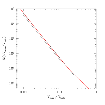
Figure 1: Theoretical cumulative abundance of non-truncated subhaloes (solid red line) for a Milky way mass halo in the concordance cosmology as a function of subhalo maximum circular velocity, $V_{\rm max}$, scaled to that of the halo. For comparison, empirical curves obtained by SWV (dashed black line) and Diemand et al. (2008) (dotted black line).

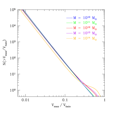
Figure 2: Same as Figure 1 but for several halo masses (coloured lines).

4 SUBHALO NUMBER DENSITY PROFILE

Given the inside-out growth of haloes formed by PA (see Sec. 2), the cumulative abundance of subhaloes with masses greater than $M_{\rm S}$ within the radius $r$, $N(<\!r,\,>\!M_{\rm S})$, must coincide with the cumulative subhalo abundance by the time the halo radius was equal to $r$. Consequently, the differential subhalo abundance, both per infinitesimal halo radius and subhalo mass, in a halo with $M_{0}$ at $t_{0}$ is

$$N(r,M_{\rm S})\!=\!\!\left(\!\!\!\left\{\!\!\left[\frac{{\rm d}N_{\delta_{\rm pk}}(M_{\rm S})}{{\rm d}\delta_{\rm pk}}\!\right]_{\!\delta({R_{\rm f}})}\!\!\!\frac{{\rm d}\delta_{\rm pk}}{{\rm d}{R_{\rm f}}}\!\right\}_{\!\!{R_{\rm f}}(M)}\!\!\!\frac{{\rm d}{R_{\rm f}}}{{\rm d}M}\!\right)_{\!\!\!M(r)}\!\!\!\!\!\frac{{\rm d}M}{{\rm d}r},$$ (23)

where

$$N_{\delta_{\rm pk}}\!(M_{\rm S})\!=\!\!\frac{M[{R_{\rm f}}(\delta_{\rm pk})]}{D(M_{\rm S})}\bigg{\{}\!N_{\rm pk}^{\rm nest}\left[{R_{\rm f}}(M_{\rm S}),\delta_{\rm pk}|{R_{\rm f}}(\delta_{\rm pk}),\delta_{\rm pk}\right]$$

$$~{}~{}~{}~{}~{}-\int_{{R_{\rm f}}(M_{\rm S})}^{{R_{\rm f}}(\delta_{\rm pk})}{\rm d}{R_{\rm f}}^{\prime}\,N_{\rm pk}^{\rm 1st\,nest}[{R_{\rm f}}(M_{\rm S}),\delta_{\rm pk}|{R_{\rm f}}^{\prime},\delta_{\rm pk}]~{}~{}~{}~{}~{}~{}$$

$$\times N_{\rm pk}^{\rm nest}[{R_{\rm f}}^{\prime},\delta_{\rm pk}\left|{R_{\rm f}}(\delta_{\rm pk}),\delta_{\rm pk}\right]\frac{M({R_{\rm f}}^{\prime})}{\bar{\rho}(t_{\rm i})}\bigg{\}},~{}~{}~{}~{}~{}~{}~{}~{}~{}~{}~{}~{}~{}$$ (24)

is the differential subhalo abundance obtained by differentiation of the cumulative subhalo abundance $N(>M_{\rm S})$, given in equation (21) for $M$ and $t$ respectively equal to $M[{R_{\rm f}}(\delta_{\rm pk})]$ and $t(\delta_{\rm pk})$, with $D(M_{\rm S})=q\left\{\pi\left[6\bar{\rho}^{2}(t_{\rm i})M_{\rm S}\right]^{2}\right\}^{1/3}$, $M(r)$ given by equation (1), ${R_{\rm f}}(M)$ given by equation (5) and ${R_{\rm f}}(\delta_{\rm pk})$ equal to the inverse typical peak trajectory solution of equation (6) leading to a halo with $M_{0}$ at $t_{0}$.

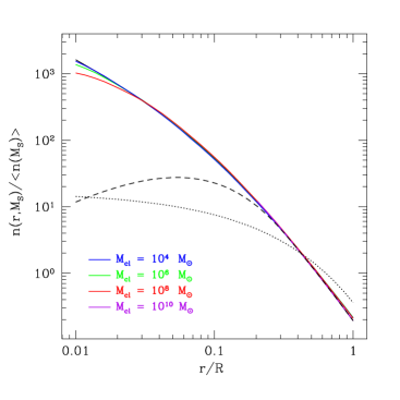
Figure 3: Theoretical non-truncated subhalo number density profiles per infinitesimal mass for subhaloes with $M_{\rm S}$, scaled to the total number, for subhaloes with different masses (solid coloured lines), compared to the halo mass density profile of the NFW profile (solid black line). The effects of including a primordial diffuse particle component that is progressively accreted by haloes is also shown (dashed coloured lines). For comparison, we also plot the Einasto law fitting the truncated subhalo number density profiles in simulated haloes (dotted black line).

In Figure 3, we show the theoretical number density profile per infinitesimal mass for subhaloes with $M_{\rm S}$, $n(r,M_{\rm S})\equiv(4\pi r^{2})^{-1}N(r,M_{\rm S})$, scaled to the total mean number density of such subhaloes, $\langle n(M_{\rm S})\rangle$, so obtained. This scaled number density profile shows a cutoff, preceded by a short bending, at small enough radii that depends on the subhalo mass (see e.g. the curves for subhaloes with $10^{8}$ M_⊙ and $10^{6}$ M_⊙). The reason for this behaviour, also found in numerical simulations (see Angulo et al. 2009), is well-understood: there can be no clump with mass $M_{\rm S}$ inside the radius $r$ encompassing that mass because the accretion of such a subhalo at the time where the halo had the mass $M(r)\sim M_{\rm S}$ would automatically cause a major merger and the consequent destruction of the merging objects. Apart from that short bending and cutoff, all the scaled number density profiles for subhaloes with different masses overlap with the mass density profile of the halo. The ratio between the subhalo number density and the total halo mass density predicted by the model (see eq. [23]),

$$\frac{n(r,M_{\rm S})}{\rho(r)}\!=\!\!\left(\!\!\left\{\!\!\left[\frac{{\rm d}N_{\delta_{\rm pk}}(M_{\rm S})}{{\rm d}\delta_{\rm pk}}\!\right]_{\!\delta_{\rm pk}({R_{\rm f}})}\!\!\!\frac{{\rm d}\delta_{\rm pk}}{{\rm d}{R_{\rm f}}}\!\right\}_{\!\!{R_{\rm f}}(M)}\!\!\frac{{\rm d}{R_{\rm f}}}{{\rm d}M}\!\right)_{\!\!M(r)}\!\!\!,$$ (25)

is flat, indeed. This result is at odds with that found in simulations, where the scaled number density profiles for subhaloes of different masses also overlap with each other, but show a much less steep profile than the halo mass density profile (see the dotted curve in Fig. 3).

The situation in simulations indicates that there is a diffuse dark matter component outside subhaloes that becomes dominant at small radii (SWV). But is this reasonable? In idealised hierarchical cosmologies, all the dark matter is expected to be locked into virialised haloes of different masses that develop through minor and major mergers. And the same is true for the matter inside haloes: all of it is expected to be locked into subhaloes of different masses. Even if subhaloes are tidally truncated by the host potential well (see Sec. 5), the liberated matter will be in the form of subhaloes previously seen as subsubhaloes. It is true that when dark matter begins to cluster, after decoupling (or after equality if decoupling took place earlier), it is in the form of a diffuse component which is accreted by the first haloes formed by monolithic collapse. But accretion of diffuse matter proceeds in a very short time compared to the cosmic times we are interested in, so we can neglect such a transient phase. In simulations, it is instead normal to find some amount of diffuse dark matter in current haloes for two reasons: i) simulations start with unclustered dark matter at much smaller redshifts (of about $100$) and ii) haloes (subhaloes) below the resolution mass contribute to a melt diffuse component until it is fully accreted by more massive haloes (subhaloes). As a consequence, only about $60$ % of the total mass in current haloes is aggregated through minor and major mergers (about $40$ and $20$ %, respectively); all the remaining mass is accreted in the form of diffuse dark matter (Wang et al., 2011). This modifies the hierarchical way CDM haloes cluster at the small mass end and leads to the presence of diffuse particles until quite a large $z$ (Angulo & White, 2010). Therefore, if we are to compare the predictions of the model with the results of $N$-body simulations, we must account for this effect.

In the presence of diffuse dark matter, the result above that the scaled subhalo number density profile overlaps with the halo mass density makes no sense. It would imply that the fraction of mass in the form of the diffuse component has the same density profile or, equivalently, that the mass fraction accreted by haloes in the form of diffuse matter is constant, whereas the diffuse dark matter should be progressively accreted, so its fraction falling into haloes should diminish with increasing time and, given the inside-out growth of accreting haloes, with increasing radius in any individual halo, causing a downward bending of the subhalo number density towards the halo centre as observed in simulated haloes.

To calculate the expected bending of the subhalo number density at small radii in a given simulation, we need to know the time-evolving mass fraction in the diffuse component outside haloes, $f_{\rm dc}(t)$. This mass fraction satisfies the differential equation

$$\frac{{\rm d}f_{\rm dc}}{{\rm d}t}=\frac{f_{\rm dc}(t)}{1-f_{\rm dc}(t)}\,\frac{1}{\bar{\rho}(t)}\int_{M_{\rm sim}}^{\infty}{\rm d}\widetilde{M}r_{\rm acc}(\widetilde{M},t)N(\widetilde{M},t)$$

$$\equiv\frac{f_{\rm dc}(t)}{1-f_{\rm dc}(t)}\,r_{\rm dc}(t)\,,~{}~{}~{}~{}~{}~{}~{}~{}~{}~{}~{}~{}~{}~{}~{}~{}~{}~{}~{}~{}~{}~{}~{}~{}~{}~{}~{}~{}~{}~{}~{}~{}~{}~{}~{}~{}~{}$$ (26)

where $r_{\rm acc}(M,t)$ is the mass accretion rate of haloes with mass $M$ at $t$, given by equation (6), and $M_{\rm sim}$ is the mass resolution of the simulation. The solution of equation (26) for the initial condition $f_{\rm dc}(t_{\rm sim})=1$, with $t_{\rm sim}$ the starting time of the simulation, is given by the implicit equation

$$f_{\rm dc}(t)-\ln[f_{\rm dc}(t)]=1-\int_{t_{\rm sim}}^{t}{\rm d}\tilde{t}\,r_{\rm dc}(\tilde{t})\,.$$ (27)

Thus, the mass accreted by the halo at $t$ in the form of subhaloes is diminished by a factor $1-f_{\rm dc}(t)$ compared to that in the case of no primordial diffuse component. Given the halo inside-out growth, this implies that the contribution from subhaloes to the halo mass density profile changes from $\rho(r)$ to $\rho(r)\{1-f_{\rm dc}[t(r)]\}$, with $t(r)$ the time where the accreting halo reaches the radius $r$. The effect of such a time varying mass fraction in the diffuse component for the initial cosmic time $t_{\rm sim}$ corresponding to $z=127$ and the resolution mass $M_{\rm sim}$ equal to $10^{4}$ M_⊙ as in SWV simulations is shown in Figure 3. The curve so obtained is much like the one found by SWV, although not identical. As we will see in Section 5, the difference is likely due to the effects of subhalo truncation not considered yet.

The presence of a diffuse dark matter component should have very little effect, however, on the cumulative subhalo abundance, $N(>M_{\rm S})$, shown in Figures 1 and 2. The reason is that, despite the outward-decreasing subhalo number density profiles, the number of subhaloes increases with radius, meaning that they are mostly aggregated by the halo at late times when essentially all the diffuse dark matter component has already disappeared (even in simulations). Only if we were analysing the subhalo abundance at very high redshifts (or very small radii) should the effect of the diffuse dark matter component also be taken into account when dealing with the subhalo abundance. Note that the same is true for the halo mass function: at very high redshifts it will be affected by the diffuse dark matter component, which should not be present in the real CDM universe. This is not taken into account in studies of that quantity from $N$-body simulations.

To sum up, in the case of (essentially) no primordial diffuse dark matter component, as in the real CDM universe, the scaled number density profile for (non-truncated) subhaloes with any given mass should coincide with the scaled halo mass density profile. On the contrary, in the case of a substantial amount of diffuse dark matter, as in numerical simulations or in the real universe soon after decoupling (or after the time of equality), the scaled number density profiles for subhaloes of different masses should also overlap with each other, but not with the halo mass density profile. They should be equal to this latter profile times the factor $1-f_{\rm dc}(r)$ giving the mass fraction clustered in haloes by the time $t(r)$ when the halo reached the radius $r$.

An important consequence of the previous result is that the spatial distribution of (non-truncated) subhaloes is the same in haloes grown by PA as in haloes having suffered major mergers. If it were different in both kinds of haloes, then the typical mass density profile would also be different, which would be in contradiction with the results of $N$-body simulations (see SVMS). Strictly, the possibility remains that the deviation in the typical mass density profile for subhaloes of some mass is exactly balanced by that for subhaloes of the remaining masses, but such an arrangement is very unnatural. We therefore conclude that the spatial distribution of subhaloes must be independent of the host aggregation history. As discussed in SVMS, this conclusion, far from being unexpected, reflects the fact that virialisation is a real relaxation process. As such, it must cause the memory loss of the initial conditions, not only regarding the smooth halo structure and kinematics, but also regarding halo substructure (but see Sec. 6).

5 THE EFFECTS OF TRUNCATION

When subhaloes are aggregated by a halo, they are tidally truncated by its potential well. Consequently, to compare the predictions of the model with the results of numerical simulations we must account for the effects of truncation. In fact, tidal truncation alters not only the mass of subhaloes but also the number of subhaloes with a given original non-truncated mass, $M_{\rm S}$, due to the appearance of new first-level subhaloes of that mass, previously seen as subsubhaloes, that are liberated from their host subhaloes.

Let us first concentrate in the change produced in the number of subhaloes with a given non-truncated mass. The number density per infinitesimal mass of subhaloes with non-truncated mass $M_{\rm S}$ corrected for the number density effect owing to truncation is

$$N^{\rm tr}(r,M_{\rm S})=N(r,M_{\rm S})+\int_{M_{\rm S}^{\rm min}}^{M}{\rm d}\widetilde{M}_{\rm S}\,N(r,\widetilde{M}_{\rm S})$$

$$\times\int_{R^{\rm tr}(r,\widetilde{M}_{\rm S})}^{R(\widetilde{M}_{\rm S})}{\rm d}\tilde{r}\,N^{\rm tr}_{\widetilde{M}_{\rm S},M(r)}(\tilde{r},M_{\rm S})\,,~{}~{}$$ (28)

where $N(r,M_{\rm S})$ is the number density of non-truncated subhaloes with mass $M_{\rm S}$, calculated in Section 4, $R^{\rm tr}(r,\widetilde{M}_{\rm S})$ is the truncation radius of the original subhaloes with mass $\widetilde{M}_{\rm S}$ located at $r$ and $M_{\rm S}^{\rm min}$ is the minimum subhalo mass that gives rise by truncation to new first-level subhaloes with $M_{\rm S}$. The subindexes in the second-level (differential) truncated subhalo abundance, $N^{\rm tr}_{\widetilde{M}_{\rm S},M(r)}(\tilde{r},M_{\rm S})$, indicate that this subhalo number density profile corrected for truncation refers to a host, in this case a subhalo, with mass $\widetilde{M}_{\rm S}$ at the time when it was aggregated by the halo, with a mass at that moment equal to $M(r)$, and hence, different from the mass $M_{0}$ of the halo at $t_{0}$.

We will consider two extreme cases. In case (a), all CDM particles are in subhaloes of a certain mass, as theoretically expected in the real CDM universe at late times, so the truncation of first-level subhaloes yields only new subhaloes previously seen as subsubhaloes; we thus have $M_{\rm S}^{\rm min}=M_{\rm S}$. In case (b), subhaloes are instead essentially made of diffuse particles, so the truncation of first-level subhaloes does not modify the number of these subhaloes (just their mass as well as the total mass of diffuse particles in the intrahalo medium); we thus have $M_{\rm S}^{\rm min}=M$. Clearly, in case (b), equation (28) has the trivial solution $N^{\rm tr}(r,M_{\rm S})=N(r,M_{\rm S})$, while in case (a) equation (28) is an integral equation neither of Fredholm nor of Volterra type, but can still be solved in the way explained in Appendix A.

The effect of truncation in the cumulative subhalo abundance as a function of $V_{\rm max}$ is shown in Figure 4. Note that the quantity $V_{\rm max}$ is insensitive to the strength of tidal truncation because the maximum circular velocity in a subhalo is reached at a radius smaller than the truncation radius. This is the reason why numerical studies usually plot the subhalo abundance as a function of $V_{\rm max}$ instead of as a function of the truncated mass much harder to estimate (see the discussion below). In case (b), truncation does not produce any apparent change in the cumulative subhalo abundance relative to that plotted in Figure 1, recovering that found in simulations. The reason is that subhaloes harbour only diffuse particles, so the subhalo number does not change where subhaloes are truncated. In contrast, we do expect an important change in case (a), better suited for the real CDM universe, owing to the appearance of new subhaloes previously seen as subsubhaloes. As shown in Figure 4, the abundance of first-level subhaloes then increases dramatically (about two orders of magnitude) in comparison with the abundance shown in Figure 1 and found in numerical simulations.

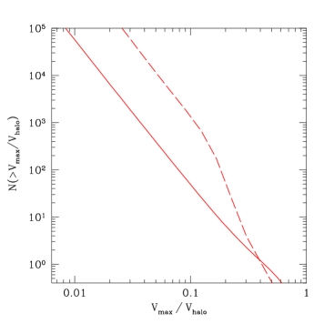
Figure 4: Same as Figure 1 but for truncated subhaloes in cases (a) (dashed red line) and (b) (solid red line) corresponding to subhaloes made of subsubhaloes (and so on) and of a diffuse particle component, respectively. The cumulative abundance of truncated subhaloes in case (a) coincides with the cumulative abundance of non-truncated subhaloes shown in Figure 1.

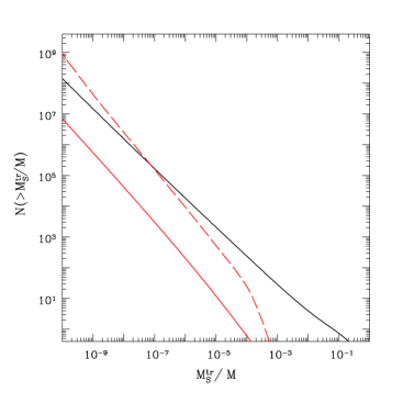
Figure 5: Same as Figure 4 but as a function of truncated mass $M_{\rm S}^{\rm tr}$. For comparison, cumulative abundance of non-truncated subhaloes (solid black line) as in Figure 1 but as a function of non-truncated mass $M_{\rm S}$ instead of maximum circular velocity $V_{\rm max}$.

All the previous results favouring case (b) indicate not only that, in simulations, a large fraction of the mass in simulated haloes is in the form of a diffuse component (see e.g. SWV), but also that such a diffuse component must be widely dominant in subhaloes so that very few new subhaloes emerge by tidal truncation of other subhaloes. This does not necessarily mean that there is no subhalo at any level higher than one. It just indicates that subsubhaloes must be rare enough for not having significant effects on the general properties of substructure as drawn from current high-resolution numerical simulations. SWV report the detection of subhaloes up to third level. However, according to the present results, these third-level subhaloes should be seen only within the most massive subhaloes and their most massive subsubhaloes, so that the total number of subhaloes liberated by truncation would be insignificant compared to the number of them directly aggregated. There are several reasons for such an important lack of subsubhaloes in simulations. Subsubhaloes are previously truncated by the subhalo potential well and this is also true for third-level subhaloes within subsubhaloes themselves and so on. The higher the level of subhaloes, the earlier they typically form and the less massive they typically are. The earlier subhaloes form, the larger is their mass fraction below the mass resolution. And, the less massive the subhaloes, the more centrally concentrated they are, so the more severe the tidal disruption they yield in their own subhaloes. Therefore, we expect the mass in simulated subhaloes to be, indeed, mostly in the form of diffuse particles.

But this is not what we expect to find in the real CDM universe with (essentially) no primordial diffuse component. Neglecting the minimum halo mass, all haloes have grown through mergers between less massive progenitors previously formed, so substructure should essentially obey case (a). The difference between the first-level subhalo abundance predicted by the model in cases (a) and (b) implies that there should be, in the real CDM universe, two orders of magnitude more first-level subhaloes than usually considered from the results of numerical simulations. This, together with the fact that in the real CDM universe the subhalo number density profile is steeper than found in simulations (see below), might have important implications on the detectability of CDM from the enhanced flux of cosmic rays produced in its annihilation in nearby subhaloes (e.g. Springel et al. 2008b; Elahi et al. 2009). However, the abundance of dwarf galaxies in, say, a Milky Way mass halo is not affected because the tidal truncation of subhaloes does not liberate new galaxies that were previously hidden. Moreover, luminous (and cold baryonic) matter usually lies at the centre of subhaloes, so the subhalo abundance relevant for the expected number of satellite galaxies rather corresponds to case (b).

We can now turn to the second effect: the change in the mass of the truncated subhaloes. To express the preceding subhalo abundance and number density profiles as a function of the subhalo truncated mass $M_{\rm S}^{\rm tr}$, we must take into account the relationship between that mass and the original non-truncated mass $M_{\rm S}$,

$$M_{\rm S}^{\rm tr}(r,M_{\rm S})=4\pi\int_{0}^{R^{\rm tr}(r,M_{\rm S})}{\rm d}\tilde{r}\,\tilde{r}^{2}\,\rho_{M_{\rm S},M(r)}(\tilde{r})\,,$$ (29)

where $\rho_{M_{\rm S},M(r)}(r)$ is the typical subhalo density profile equal to that for haloes with mass $M_{\rm S}$ at the time of the subhalo aggregation when the halo had a mass equal to $M(r)$.

The cumulative abundances of truncated subhaloes for Milky Way mass haloes as a function of $M_{\rm S}^{\rm tr}$ are plotted in Figure 5. The log-log slopes we find are equal to $-1.12$ and $-1.05$ for cases (a) and (b), respectively (or $-2.12$ and $-2.05$ for the differential subhalo abundance). The slope found by SWV in their numerical simulations was $-0.90\pm 0.03$ ($-1.90\pm 0.03$), hence once again closer to the value predicted by the model in case (b). Note that, although the difference between the theoretical and empirical slopes in case (b) is small, it may be essential for having a convergent or divergent number of subhaloes for masses approaching to zero. It is true that this limit is actually not reached due to the cutoff in the power-spectrum (and the non-negligible velocity dispersion) of dark matter particles, but those slopes still tell at which extent the mass fraction in low-mass subhaloes is dominant or not. The possible origin of the slight departure in the slope between the predictions of the model and the results of numerical simulations is discussed below. In any case, even if the total number of subhaloes in case (b) converged, that in case (a) should diverge as found here, so our results point, in the case of CDM cosmologies, to a halo mass fraction in the form of low-mass subhaloes (below the resolution of current simulations) much larger than usually thought.

The subhalo number density per infinitesimal mass corrected for truncation as a function of the truncated subhalo mass, $M_{\rm S}^{\rm tr}$, or simply the real truncated subhalo number density per infinitesimal mass, takes the form

$$N^{\rm tr}(r,M_{\rm S}^{\rm tr})=N[r,M_{\rm S}(r,M_{\rm S}^{\rm tr})]+\int_{M_{\rm S}^{\rm min}}^{M}{\rm d}\widetilde{M}_{\rm S}\,N(r,\widetilde{M}_{\rm S})$$

$$\times\int_{R^{\rm tr}(r,\widetilde{M}_{\rm S})}^{R(\widetilde{M}_{\rm S})}{\rm d}\tilde{r}\,N^{\rm tr}_{\widetilde{M}_{\rm S},M(r)}(\tilde{r},M_{\rm S}^{\rm tr})\,,~{}~{}~{}~{}~{}~{}~{}~{}~{}~{}~{}$$ (30)

with the function $M_{\rm S}(r,M_{\rm S}^{\rm tr})$ implicitly defined by equation (29). The integral equation (30) can be solved for $N^{\rm tr}(r,M_{\rm S}^{\rm tr})$ in the two extreme cases (a) and (b) above in the same way as equation (28) for $N^{\rm tr}(r,M_{\rm S})$. Note that the truncation radius $R^{\rm tr}$ in equations (28) and (30) depends, for a given halo mass, not only on the radius of the subhalo at the aggregation time and its non-truncated mass, but also on its orbit, which in turn depends on the host kinematics, modelled in SSMG.

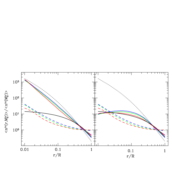
Figure 6: Same as Figure 3 but for truncated subhalo masses $M_{\rm S}^{\rm tr}$, in the same cases (a) (dashed lines) and (b) (solid lines) as in previous figures, compared now to the Einasto law (solid black line) that fits the subhalo number density profiles drawn from simulations (SWV). For comparison with Figure 3, we also plot the NFW law fitting the predicted number density of non-truncated subhaloes (dotted black line). Left panel: predictions for the case of no primordial diffuse particle component. Right panel: case (b) predictions for the case of a primordial diffuse particle component that is progressively accreted by haloes.

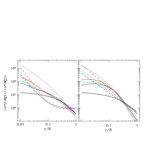
Figure 7: Same as right panel of Figure 6 but using the Zhao et al. (2009) (left panel) and Klypin et al. (2011) (right panel) $M$-$c$ toy models instead of the SMGH physical model to calculate the effects of subhalo truncation by the host potential well.

The truncation radius is very hard to determine in numerical simulations. This is why different authors adopt different procedures leading to somewhat different results. For instance, Diemand et al. (2007) took the radius at which the density of the subhalo (corrected for the local background contribution) is equal to the local background density, while SWV adopted the radius at which the clump mean inner density (also corrected for the local background contribution) is 0.02 times the mean inner background density, shown to lead to a truncation radius in overall agreement with the theoretical tidal radius defined by Binney & Tremaine (1987). In the present model, we adopt the better motivated truncation radius given in Gonzalez-Casado et al. (1994). These authors showed that, regardless of the shape of the orbit, subhaloes are truncated by the host potential well essentially at the radius encompassing an inner mean density equal to that of the host halo at the clump pericentre. Note that such a truncation radius would roughly coincide with Diemand et al.’s provided clumps described circular orbits; unfortunately, this is not the case in general. On the other hand, it would coincide with SWV. truncation radius provided the halo mean inner density at the subhalo pericentre were 0.02 times the local halo density, which is, in general, not the case either. Assuming subhaloes with the median velocity for a normal distribution with radial and tangential velocity dispersions given by the model in SSMG, we determined the typical pericentre reached by subhaloes located at any given radius. Then, assuming the non-truncated subhaloes at their aggregation time with the typical halo density profile with the mass-concentration ($M$–$c$) relation given by Salvador-Solé et al. (2007, hereafter SMGH), we calculated, from the halo mean inner density at the resulting subhalo pericentre, the wanted subhalo truncation radius.

Figure 6 shows the theoretical number density profile per infinitesimal mass for truncated subhaloes with $M^{\rm tr}_{\rm S}$, scaled to the total number of such subhaloes for Milky Way mass haloes in cases (a) and (b) compared to those found in numerical simulations or, more exactly, to the shallow profile of the Einasto form fitting them. In numerical simulations, these scaled number density profiles are indeed found to be much shallower than the halo density profile (Diemand et al. 2004b; Gao et al. 2004; Nagai & Kravtsov 2005; Diemand et al. 2007; SWV) and independent of subhalo mass (Diemand et al. 2004a; SWV; Ludlow et al. 2009). In the left panel of Figure 6, we see that the truncated subhalo number density profiles predicted by the model in case (a), with no primordial diffuse component, are on the contrary similarly steep as the NFW profile fitting the profiles found for non-truncated subhaloes and show now a slight dependence on subhalo mass. The situation does not improve in case (b): the number density profiles show a more marked dependence on subhalo mass and are much shallower than found in simulations at large radii, while they become steeper at small radii. And an intermediate case between (a) and (b) would not improve the results: the theoretical number density profiles would always show a clear dependence on $M^{\rm tr}_{\rm S}$ and be convex instead of concave.

As mentioned, the fact that the empirical subhalo number density profiles are independent of subhalo mass and shallower than the halo mass density profile implies that, in numerical simulations, a substantial fraction of dark matter is in the form of a diffuse component that increases inwards. According to the discussion in Section 4, a bending of the theoretical number density profiles towards those found in simulations is expected, indeed, in the case that there is a primordial diffuse component that is progressively accreted by haloes. Such an effect was calculated in Section 4 for non-truncated haloes. Thus, we have repeated the same calculations for truncated haloes in case (b) (in case (a) there is no diffuse component). That is, we have considered that the contribution of subhaloes to the halo mass density is given by $\rho(r)[1-f_{\rm dc}(r)]$ instead of $\rho(r)$. Then, the log-log slope of the truncated subhalo abundance does not essentially change, but the truncated subhalo number density profiles do markedly. As shown in the right panel of Figure 6, they then become essentially in agreement with the results of numerical simulations.

The small deviations that still remain (in the curvature of the profiles and in the dependence on subhalo mass) are likely due to the SMGH $M$–$c$ relation used in the modelling of truncation for very large $z$, which apparently is not accurate enough. To see the kind of effect the adoption of one particular $M$–$c$ relation has on these results, we have repeated the same calculation with two different $M$–$c$ relations: those provided by Klypin et al. (2011) and Zhao et al. (2009). The predicted log-log slopes of the differential truncated subhalo abundance are then equal to $-2.07$ and $-2.01$ using Klypin et al. $M$–$c$ relation and $-2.04$ and $-2.01$ using Zhao et al. $M$–$c$ relation for cases (a) and (b), respectively (to be compared with the slopes of $-2.12$ and $-2.05$ found using the SMGH $M$–$c$ relation and the slope of $-1.9$ found in numerical simulations by SWV). The truncated subhalo number density profiles in case (b) predicted using Klypin et al. (2011) and Zhao et al. (2009) $M$–$c$ relations are shown in Figure 7. As can be seen, the theoretical subhalo number density profiles so obtained deviate more markedly from the profiles drawn from simulations and are more mass-dependent than those shown in the right panel of Figure 6. Therefore, the predictions drawn from the SMGH $M$–$c$ relation are neatly preferable. It may seem strange that the $M$–$c$ relations drawn from numerical simulations give poorer results than those derived from the SMGH model. We note, however, that Klypin et al. (2011) and Zhao et al. (2009) $M$–$c$ relations do not actually fit the results of simulations; they are the extrapolations of the real fitting expressions, through some guessed toy models, to the much wider mass and $z$ domains involved in the present calculations. In any event, these results clearly show that any slight deviation of the $M$–$c$ from the true relation has notable effects, indeed, in the theoretical truncated subhalo number density profile.

Before concluding this Section, it is important to remark that, as the non-truncated subhalo number density profile, $N(r,M_{\rm S}^{\rm tr})$, is independent of the halo aggregation history (see Sec. 4) and so are also both the anisotropy and velocity dispersion profiles (SSMG) and the mass density profiles (SVMS) setting the truncation radii, the truncated subhalo number density profiles, $N^{\rm tr}(r,M_{\rm S}^{\rm tr})$, must be also independent of the halo aggregation history. In other words, all the properties derived so far should not depend on the halo aggregation history. This would explain why all substructure properties derived from numerical simulations reporting to haloes with very different aggregation histories, show such small scatters.

6 THE EFFECTS OF DYNAMICAL FRICTION

But things are not that simple. The spatial distribution of subhaloes is also affected by dynamical friction resulting from gravitational two-body interactions between subhaloes themselves and between subhaloes and diffuse dark matter particles. As in a major merger, the radial location of subhaloes suffers an important scrambling, the effects of dynamical friction that have previously taken place are essentially erased. Therefore, the effects of dynamical friction depend on the time elapsed since the last major merger. This means that, contrarily to all the processes previously mentioned, dynamical friction may lead to significant differences between haloes according to their aggregation history (through the time elapsed since the last major merger).

The large number of tiny subhaloes and of diffuse dark matter (in numerical simulations) suggests that dynamical friction should be very effective, at least in the case of the most massive subhaloes more prone to suffer it. But, this should have repercussions on the smooth structure and kinematics of haloes, which should then depend on the halo aggregation history, while there is no clear sign of such a dependence in simulations (see SVMS and references therein). Furthermore, as a consequence of dynamical friction, the most massive subhaloes should lie closer to the halo centre than less massive ones, whereas subhaloes of different masses show identical scaled number density profiles. And the only minor difference is rather of the opposite sign: the more massive the subhalo, the larger the minimum radius reached by its scaled number density profile (Angulo et al., 2009). In particular, there is no sign of very massive haloes being accumulated at the halo centre. Therefore, simulated haloes show no apparent effect of dynamical friction.

The only way to escape this paradox seems to be that the effects of dynamical friction may be present but go unnoticed. Does this make sense? If the only subhaloes having had time to suffer significant dynamical friction since the last major merger were the most massive ones, it could be very difficult to detect it because the number of those subhaloes is so small that their number density profile is quite uncertain (due to large Poisson errors). Certainly, they could be quite numerous at the halo centre where they should tend to accumulate, but, when a very massive subhalo falls to the halo centre and merges with the massive subhalo already lying there or simply settles down well-centred, it becomes invisible because it mimics the central part of the host halo. This effect could still manifest itself through an increased amount of small subhaloes near the halo centre, corresponding to old second-level subhaloes (in the massive subhaloes having fallen to the halo centre) converted to first-level ones. But such an effect should only be observable in case (a), because, in case (b), subhaloes are mainly made of diffuse dark matter. In this sense, the lack of such an indirect proof of dynamical friction would be an additional argument in favour of case (b) when trying to model the results of $N$-body simulations.

7 SUMMARY AND CONCLUSIONS

The evolution of nested peaks in the filtering of the primordial density field truthfully traces the evolution of halo substructure developing at all levels as a consequence of halo accretion and major mergers. Thus, the peak formalism can be used to describe subhalo abundance in typical haloes. Moreover, taking into account that haloes growing by PA develop from the inside out, it can be used to derive the non-truncated subhalo number density profiles per infinitesimal mass for subhaloes of different masses and, making use of the halo structural and kinematic profiles modelled in SVMS and SSMG, one can correct those quantities from tidal truncation as well.

The subhalo properties predicted in the $\Lambda$CDM cosmology for Milky Way mass haloes are in very good agreement with those found in numerical simulations provided dark matter within subhaloes is essentially in the form of diffuse particles. The only slight deviations found, in this case, between the theoretical predictions and the results of numerical simulations seem to be due to the non-fully accurate (sub)halo $M$–$c$ relation used. More accurate $M$–$c$ relations drawn e.g. from the SVMS model of halo structure would be welcome.

But the true subhalo properties expected on pure theoretical grounds in a real CDM universe rather correspond to those predicted under the opposite assumption that all dark matter in subhaloes is locked in higher-order level subhaloes. Accurate predictions are also given for this more realistic case. The most striking result is that there should be, in this case, two orders of magnitude more subhaloes than usually thought on the basis of the results of $N$-body simulations. This might have important implications for the detectability of CDM, but it does not affect the dwarf galaxy abundance estimated from CDM simulations.

In any of these two scenarios, subhalo properties are expected to be independent of the halo aggregation history. This means that, despite having been derived under the PA condition, all the previous quantities should hold for haloes having suffered major mergers. The only effects that could depend on the halo aggregation history are those due to dynamical friction. According to the present results and those found in SVMS and SSMG, dynamical friction can be neglected as long as we are interested in modelling haloes in current simulations. However, it might have visible effects in the real CDM universe as well as in future, higher resolution, $N$-body simulations. Of course, dynamical friction is also expected to have important consequences in baryon physics ignored in the present study.

ACKNOWLEDGEMENTS

This work was supported by the Spanish DGES, AYA2006-15492-C03-03 and AYA2009-12792-C03-01, and the Catalan DIUE, 2009SGR00217. One of us, SS, was beneficiary of a grant from the Institut d’Estudis Espacials de Catalunya.

Appendix A TRUNCATED SUBHALO NUMBER DENSITY IN CASE (a)

In case (a), i.e. $M_{\rm S}^{\rm min}=M_{\rm S}$, the subhalo number density per infinitesimal mass corrected for truncation (eq. [28]) takes the form

$$N^{\rm tr}(r,M_{\rm S})=N(r,M_{\rm S})+\int_{M_{\rm S}}^{M}{\rm d}\widetilde{M}_{\rm S}\,N(r,\widetilde{M}_{\rm S})\int_{R^{\rm tr}(r,\widetilde{M}_{\rm S})}^{R(\widetilde{M}_{\rm S})}{\rm d}\tilde{r}\,N^{\rm tr}_{\widetilde{M}_{\rm S},M(r)}(\tilde{r},M_{\rm S})\,.$$ (31)

By partial integration, equation (31) leads to

$$N(r,M_{\rm S})=N(r,M_{\rm S})+\int_{M_{\rm S}}^{M}{\rm d}\widetilde{M}_{\rm S}\,N(r,>\widetilde{M}_{\rm S})\frac{{\rm d}}{{\rm d}\widetilde{M}_{\rm S}}\int_{R^{\rm tr}(r,\widetilde{M}_{\rm S})}^{R(\widetilde{M}_{\rm S})}{\rm d}\tilde{r}\,N^{\rm tr}_{\widetilde{M}_{\rm S},M(r)}(\tilde{r},M_{\rm S})\,.$$ (32)

Taking into account that both expressions (31) and (32) hold for any arbitrary value of $M_{\rm S}$, we are led to

$$\frac{{\rm d}\ln}{{\rm d}\widetilde{M}_{\rm S}}[N(r,<\widetilde{M}_{\rm S})]=\frac{{\rm d}\ln}{{\rm d}\widetilde{M}_{\rm S}}\int_{R^{\rm tr}(r,\widetilde{M}_{\rm S})}^{R(\widetilde{M}_{\rm S})}{\rm d}\tilde{r}\,N^{\rm tr}_{\widetilde{M}_{\rm S},M(r)}(\tilde{r},M_{\rm S})\,,$$ (33)

implying

$${\Re}(r,M_{\rm S})N(r,<\widetilde{M}_{\rm S})=\int_{R^{\rm tr}(r,\widetilde{M}_{\rm S})}^{R(\widetilde{M}_{\rm S})}{\rm d}\tilde{r}\,N^{\rm tr}_{\widetilde{M}_{\rm S},M(r)}(\tilde{r},M_{\rm S})\,,$$ (34)

where the function ${\Re}(r,M_{\rm S})$ is the unknown integration constant. Choosing $\widetilde{M}_{\rm S}$ equal to $M(r)$ and taking into account that haloes grow inside-out, the double subindex “$\widetilde{M}_{\rm S},M(r)$” in the truncated subhalo number density in the integrand on the right can be chosen equal to “$M_{0},M_{0}$” without any loss of generality (see the meaning of such a double subindex in eq. [28]). That is, for that particular value of $\widetilde{M}_{\rm S}$, the subhalo is a clone of the host halo, except for the fact that it has not grown since it was aggregated by the host halo. In particular, its (sub)subhalo number density corrected for truncation is identical to that of the host halo itself (the subindex “$M_{0},M_{0}$” can be omitted) and the (sub)subhalo with mass $M_{\rm S}$ is found at the same minimum radius $r(M_{\rm S})$ as in the host halo. Consequently, equation (34) takes the form

$${\Re}(r,M_{\rm S})N(r)=\int^{r}_{{\rm max}\{r(M_{\rm S}),R^{\rm tr}[r,M(r)]\}}{\rm d}\tilde{r}\,N^{\rm tr}(\tilde{r},M_{\rm S})\,,$$ (35)

where we have taken into account that the $N[r,<M(r)]$ is but the total subhalo number density at $r$, denoted as $N(r)$.

At small $r$, we have $r(M_{\rm S})\geq R^{\rm tr}[r,M(r)]$ and differentiation of equation (35) leads to

$$N^{\rm tr}(r,M_{\rm S})=\frac{{\rm d}}{{\rm d}r}\left[{\Re}(r,M_{\rm S})N(r)\right]\,.$$ (36)

Substituting $N^{\rm tr}(r,M_{\rm S})$ given by equation (36) into equation (31), taking into account equation (34) and the partial integration of the $\widetilde{M}_{\rm S}$-integral in the resulting expression, we arrive at

$$\frac{{\rm d}}{{\rm d}r}\left[{\Re}(r,M_{\rm S})N(r)\right]=N(r,M_{\rm S})+\frac{1}{2}{\Re}(r,M_{\rm S})N(r)\,N(r,>M_{\rm S})\,\left[2-\frac{N(r,>M_{\rm S})}{N(r)}\right]\,.$$ (37)

For any reasonable (large enough) value of $M_{\rm S}$, $N(r,>M_{\rm S})/N(r)$ is negligible in front of unity, so equation (37) takes the simple form

$$\frac{{\rm d}}{{\rm d}r}\left[{\Re}(r,M_{\rm S})N(r)\right]=N(r,M_{\rm S})+\left[{\Re}(r,M_{\rm S})N(r)\right]\,N(r,>M_{\rm S})\,.$$ (38)

This is a differential equation for ${\Re}(r,M_{\rm S})$, which can be solved for the initial condition ${\Re}[r(M_{\rm S}),M_{\rm S}]=0$ implied by equation (35). Then, replacing the solution ${\Re}(r,M_{\rm S})$ into equation (36), we obtain the wanted number density per infinitesimal mass of truncated subhaloes, $N^{\rm tr}(r,M_{\rm S})$.

At a large enough $r$, hereafter denoted by $r_{\rm end}$, the condition $r(M_{\rm S})<R^{\rm tr}[r,M(r)]$ will be finally met and this solution will no longer hold. In this new regime, differentiation of equation (35) leads to

$$N^{\rm tr}(r,M_{\rm S})=\frac{{\rm d}}{{\rm d}r}\left[{\Re}(r,M_{\rm S})N(r)\right]-\frac{{\rm d}R^{\rm tr}[r,M(r)]}{{\rm d}r}\,N^{\rm tr}\{R^{\rm tr}[r,M(r)],M_{\rm S}\}\,.$$ (39)

Substituting $N^{\rm tr}(r,M_{\rm S})$ given by equation (39) into equation (31), taking into account equation (34) and integrating by parts the integral over $\widetilde{M}_{\rm S}$ in the resulting expression, we obtain

$$\frac{{\rm d}}{{\rm d}r}\left[{\Re}(r,M_{\rm S})N(r)\right]+\frac{{\rm d}R^{\rm tr}[r,M(R)]}{{\rm d}r}\,N^{\rm tr}\{R^{\rm tr}[r,M(r)],M_{\rm S}\}~{}~{}~{}~{}~{}~{}~{}~{}~{}~{}~{}~{}~{}~{}~{}~{}~{}~{}~{}~{}~{}~{}~{}~{}~{}$$

$$=N(r,M_{\rm S})+\frac{1}{2}\,{\Re}(r,M_{\rm S})\,N(r)\,N(r,>M_{\rm S})\,\left[2-\frac{N(r,>M_{\rm S})}{N(r)}\right]\,$$ (40)

which, for any reasonable (large enough) value of $M_{\rm S}$, reduces to

$$\frac{{\rm d}}{{\rm d}r}\left[{\Re}(r,M_{\rm S})N(r)\right]+\frac{{\rm d}R^{\rm tr}[r,M(R)]}{{\rm d}r}\,N^{\rm tr}\{R^{\rm tr}[r,M(r)],M_{\rm S}\}$$

$$=N(r,M_{\rm S})+\left[{\Re}(r,M_{\rm S})N(r)\right]\,N(r,>M_{\rm S})\,.$$ (41)

As $R^{\rm tr}[r,M(r)]$ is smaller than $r$, the function $N^{\rm tr}\{R^{\rm tr}[r,M(r)],M_{\rm S}\}$ has been previously obtained in the range of small $r$, so the differential equation (41) can then also be solved for the function ${\Re}(r,M_{\rm S})$ with the initial condition given by the value of ${\Re}(r,M_{\rm S})$ at $r_{\rm end}$. Once ${\Re}(r,M_{\rm S})$ has been determined, we can replace it in equation (39) to obtain the wanted function $N^{\rm tr}(r,M_{\rm S})$ in the new radial range.

In fact, given that $r(M_{\rm S})$ is greater than $R^{\rm tr}\{R^{\rm tr}(r,M_{\rm S}),M[R^{\rm tr}(r,M_{\rm S})]\}$ in the relevant subhalo mass range (i.e. except for $M_{\rm S}\la 10^{3}$ M_⊙), the differential equation (41) can be solved analytically. Indeed, equation (34) for $r=R^{\rm tr}(r,M_{\rm S})$ then takes the form

$${\Re}[R^{\rm tr}(r,M_{\rm S}),M_{\rm S})]N(r)=\int^{R^{\rm tr}(r,M_{\rm S})}_{r(M_{\rm S})}{\rm d}\tilde{r}\,N^{\rm tr}(\tilde{r},M_{\rm S})\,.$$ (42)

Thus, by differentiating it with respect to $R^{\rm tr}(r,M_{\rm S})$ and replacing the resulting expression for $N^{\rm tr}\{R^{\rm tr}[r,M(r)],M_{\rm S}\}$ into equation (41), we arrive at

$$\frac{{\rm d}\ln}{{\rm d}\ln r}\left[{\Re}(r,M_{\rm S})N(r)\right]=r\left\{1-\frac{1-N(r,M_{\rm S})/\left[{\Re}(r,M_{\rm S})N(r)\right]}{1+N(r,>M_{\rm S})}\right\}\,.$$ (43)

$N(r,M_{\rm S})$ is much smaller than $N(r)$ and ${R_{\rm f}}(r,M_{\rm S})$ is much greater than one in this radial range, except for $M_{\rm S}\ga 10^{10}$ M_⊙, as is checked a posteriori from equation (35). Consequently, for $M_{\rm S}<10^{10}$ M_⊙ we can neglect the term $N(r,M_{\rm S})/[{\Re}(r,M_{\rm S})N(r)]$ on the right of equation (43), which leads to the following quite accurate solution

$${\Re}(r,M_{\rm S})N(r)=A(r_{\rm end})\,\exp\left[\int_{r_{\rm end}}^{r}{\rm d}\tilde{r}\,\,\frac{N(\tilde{r},>M_{\rm S})}{1+N(\tilde{r},>M_{\rm S})}\right]\,,$$ (44)

with $A(r_{\rm end})$ an integration constant whose value is obtained by continuity of the solution at $r_{\rm end}$. Finally, differentiating equation (44) and taking into account equation (34) we are led to

$$N^{\rm tr}(r,M_{\rm S})=\frac{A(r_{\rm end})\,N(r,>M_{\rm S})}{1+N(r,>M_{\rm S})}\exp\left[\int_{r_{\rm end}}^{r}{\rm d}\tilde{r}\,\,\frac{N(\tilde{r},>M_{\rm S})}{1+N(\tilde{r},>M_{\rm S})}\right]\,.$$ (45)

References

- Angulo et al. (2009) Angulo R. E., Lacey C. G., Baugh C. M., Frenk C. S., 2009, MNRAS, 399, 983
- Angulo & White (2010) Angulo R.E. & White S. D. M., 2010, MNRAS, 401, 1796
- Bardeen et al. (1986) Bardeen J. M., Bond J. R., Kaiser N., Szalay A. S., 1986, ApJ, 304, 15 (BBKS)
- Belokurov et al. (2006) Belokurov V., Evans N. W., Irwin M. J., Hewett P. C., Wilkinson M. I., 2006, ApJ, 637, L29
- Binney & Tremaine (1987) Binney J. & Tremaine S. D., 1987,Galactic dynamics, Princeton University Press
- Bullock et al. (2010) Bullock J. S., Stewart K. R., Kaplinghat M., Tollerud E. J., Wolf J., 2010, ApJ, 717, 1043
- Bond & Myers (1996) Bond, J. R. & Myers S. T., 1996, ApJS, 103, 41
- Boylan-Kolchin et al. (2011) Boylan-Kolchin M., Bullock J. S., Kaplinghat M., 2011, MNRAS, 415, L40
- Bryan & Norman (1998) Bryan G.L. & Norman M. L., 1998, ApJ, 495, 80
- De Lucia et al. (2004) De Lucia G. et al., 2004, MNRAS, 348, 333
- Diemand et al. (2004a) Diemand J., Moore B., Stadel J., 2004a, MNRAS, 353, 624
- Diemand et al. (2004b) Diemand J., Moore B., Stadel J., 2004b, MNRAS, 352, 535
- Diemand et al. (2007) Diemand J., Kuhlen M., Madau P., 2007, ApJ, 657, 267
- Diemand et al. (2008) Diemand J., Kuhlen M., Madau P., Zemp M., Moore B., Potter D., Stadel J., 2008, Nature, 454, 735
- Doroshkevich (1970) Doroshkevich A. G., 1970, Astrofizika, 6, 581
- Doroshkevich & Shandarin (1978) Doroshkevich A. G. & Shandarin S. F., 1978, MNRAS, 182, 27
- Einasto (1965) Einasto J., 1965, Trudy Inst. Astrofiz. Alma-Ata, 5, 87
- Elahi et al. (2009) Elahi, P. J., Widrow, L. M., Thacker, R. J., 2009, Ph. Rev. D, 80, 123513
- Fujita et al. (2002) Fujita Y., Sarazin C. L., Nagashima M., Yano T., 2002, ApJ, 577, 11
- Gao et al. (2004) Gao L, White S. D. M., Jenkins A., Stoehr F., Springel V., 2004, MNRAS, 355, 819
- Gao et al. (2005) Gao L., Springel V., White, S. D. M., 2005, MNRAS, 363, L66
- Gao et al. (2011) Gao L, Frenk C. S., Boylan-Kolchin M., Jenkins A., Springel V., White S. D. M., 2011, MNRAS, 410, 2309
- Ghigna et al. (1998) Ghigna S., Moore B., Governato F., Lake G., Quinn T., Stadel J., 1998, MNRAS, 300, 146
- Gonzalez-Casado et al. (1994) Gonzalez-Casado G., Mamon G. A., & Salvador-Sol, E. 1994, ApJ, 433, L61
- Helmi et al. (2002) Helmi A., White S. D. M., Springel V., 2002, Phys. Rev. D, 66, 063502
- Klypin et al. (1999) Klypin A., Gottöber S., Kravtsov A. V., 1999, ApJ, 516, 530
- Klypin et al. (2011) Klypin A., Trujillo-Gómez, S., Primack, J., 2011, ApJ, 740, 102
- Komatsu et al. (2011) Komatsu E., Smith K. M., Dunkley J., Bennet C. L., Gold B., Hinshaw G., Jarosik N., Larson D., and 13 others, 2011, ApJS, 192, 18
- Koposov et al. (2010) Koposov S. E., Rix H., Hogg D. W., 2010, ApJ, 712, 260
- Kravtsov et al. (2004) Kravtsov A. V., Berlind A., Wechsler R. H., Klypin A. A., Gottlöber S., Allgood B., Primack J. R., 2004, ApJ, 609, 35
- Lovell et al. (2012) Lovell M. R., Eke V., Frenk C. S., Gao L., Jenkins A., Theuns, T., Wang J., Boyarsky A., Ruchaysiy O., 2012, MNRAS, 420, 2318
- Ludlow et al. (2009) Ludlow A. D., Navarro J. F., Springel V., Jenkins A., Frenk C. S., Helmi A., 2009, ApJ, 692, L931
- Manrique & Salvador-Solé (1995) Manrique A. & Salvador-Sole E., 1995, ApJ, 453, 6 (MSSa)
- Manrique & Salvador-Solé (1996) Manrique A. & Salvador-Sole E., 1996, ApJ, 467, 504 (MSSb)
- Manrique et al. (1998) Manrique A., Raig A., Solanes J. M., González-Casado G., Stein, P., Salvador-Solé E., 1998, ApJ, 499, 548
- Moore et al. (1999) Moore B., Ghigna S., Governato F, Lake G., Quinn T., Stadel J., Tozzi P., 1999, ApJ, 524, L19
- Nagai & Kravtsov (2005) Nagai, D., & Kravtsov, A. V. 2005, ApJ, 618, 557
- Navarro et al. (1997) Navarro J. F., Frenk C. S. & White S. D. M., 1997, ApJ, 490, 493
- Oguri & Lee (2004) Oguri M. & Lee J. 2004, MNRAS, 355, 120
- Peacock & Heavens (1990) Peacock, J. A. & Heavens A. F., 1990, MNRAS, 243, 133
- Reed et al. (2005) Reed D., Governato F., Quinn T., Gardner J., Stadel J., Lake G., 2005, MNRAS, 359, 1537
- Salvador-Solé et al. (2007) Salvador-Solé E., Manrique A., González-Casado G., Hansen S. H., 2007, ApJ, 666, 181 (SMGH)
- Salvador-Solé et al. (2012a) Salvador-Solé E., Viñas J., Manrique A., Serra S., 2012, accepted for publication in MNRAS (SVMS)
- Salvador-Solé et al. (2012b) Salvador-Solé E.,Serra S., Manrique A., González-Casado, G., 2012, submitted to MNRAS (SSMG)
- Sheth (2003) Sheth R. K., 2003, MNRAS, 345, 1200
- Strigari et al. (2010) Strigari L.E., Frenk C. S., White S. D. M., 2010, MNRAS, 408, 2364
- Springel et al. (2001) Springel V., White S. D. M.,Tormen G., Kauffmann G., 2001, MNRAS, 328, 726
- Springel et al. (2008a) Springel V., Wang J., Vogelsberger M., et al., 2008a, MNRAS, 391, 1685 (SWV)
- Springel et al. (2008b) Springel V., White S. D. M., Frenk C. S., et al., 2008b, Nature, 456, 73
- Stoehr et al. (2003) Stoehr F., White S. D. M.,Springel V., Tormen G., Yoshida. N., 2003, MNRAS, 345, 1313
- Vera-Ciro et al. (2011) Vera-Ciro C. A., Sales L. V., Helmi A., Frenk C. S., Navarro J. F., Springel V., Vogelsberger M., White S. D., 2011, MNRAS, 416, 1377
- Wang et al. (2011) Wang J., Navarro J. F., Frenk C. S., et al. 2011, MNRAS, 413, 1373
- Wechsler et al. (2002) Wechsler R. H., Bullock J. S., Primack J. R., Kravtsov A. V., Dekel A., 2002, ApJ, 568, 52
- Williams & McKee (1997) Williams J. P., McKee, C. F., 1997, ApJ, 476, 166
- Zhao et al. (2009) Zhao D. H., Jing Y. P., Mo H. J., Börner G., 2009, ApJ, 707, 354