CUQM - 139
Study of the generalized quantum isotonic nonlinear oscillator potential
Abstract
We study the generalized quantum isotonic oscillator Hamiltonian given by , . Two approaches are explored. A method for finding the quasi-polynomial solutions is presented, and explicit expressions for these polynomials are given, along with the conditions on the potential parameters. By using the asymptotic iteration method we show how the eigenvalues of this Hamiltonian for arbitrary values of the parameters and may be found to high accuracy.
keyword: Non-linear oscillators; Non-polynomial potentials; Gol’dman and Krivchenkov potential; Asymptotic Iteration Method; Quantum integrable systems; Laguerre polynomials.
PACS: 03.65.w, 03.65.Fd, 03.65.Ge.
I Introduction
Recently, Cariñena et al. Carinena studied a quantum nonlinear oscillator potential whose Schrödinger equation reads
| (1) |
The interest in this problem came from the fact that it is exactly solvable, in a sense that the exact eigenenergies and eigenfunctions can be obtained explicitly. Indeed, Cariñena et al. Carinena were able to show that
| (2) |
where the polynomials factors are related to the Hermite polynomials by means of
| (3) |
In a more recent work, Fellows and Smith fellows showed that the potential as well as, for certain values of the parameters , and , the potential of the Schrödinger equation
| (4) |
are indeed supersymmetric partners of the harmonic oscillator potential. Using the supersymmetric approach, the authors were able to construct an infinite set of exact soluble potentials, along with their eigenfunctions and eigenvalues. Very recently, Sesma sesma , using a Möbius transformation, was able to transform Eq.(4) into a confluent Heun equation heun and thereby obtain an efficient algorithm to solve the Schrödinger equation (4) numerically. The purpose of the present work is to provide a detailed solution, by means of the quasi-polynomial solutions and the application of the asymptotic iteration method brodie ; C3 ; ciftci1 ; ciftci2 , for the Schrödinger equation
| (5) |
where is the angular momentum number . Our results show that the quasi-exact solutions of Sesma sesma as well the results of Cariñena et al. Carinena follow as special cases of our general approach. The present article is organized as follows. In the next section, some preliminary analysis of the Schrödinger equation (5) is presented. A general approach for finding polynomial solutions of Eq.(5), for certain values of parameters and , is presented, and is based on a recent work of Ciftci et al. C3 for solving the second-order linear differential equation
| (6) |
More general quasi-exact solutions, including the results of Sesma sesma , are discussed in section III. Unrestricted solutions of Eq.(5) based on the asymptotic iteration method are discussed in Section IV.
II Generalized quantum isotonic oscillator - preliminary results
A simple scaling argument, using , allows us to write the equation (5) as
| (7) |
A further substitution yields a differential equation with two regular singular points at and one irregular singular point of rank at . The roots ’s of the indicial equation for the regular singular point reads , while the roots of the indicial equation at are and . Since the singularity for corresponds to that for , it is necessary that the solution for behave as . Consequently, we may assume the general solution of equation (7) which vanishes at the origin and at infinity takes the form
| (8) |
A straightforward calculation shows that are the solutions of the second-order homogeneous linear differential equation
| (9) |
In the next sections, we attempt to give a general solution of this equation. For now, we assume that takes the value of the indicial root
| (10) |
which allows us to write Eq.(II) as
| (11) |
We now consider the cases where the following two equations are satisfied
The solutions of this system, for and , are given explicitly by
| (12) |
In the next, we consider each case of these two sets of solutions.
II.1 Case 1
The first set of solutions reduces the differential equation (II) to
| (13) |
which is a special case of the general differential equation
| (14) |
with , , , and . The necessary and sufficient conditions for polynomial solutions of Eq.(14) are given by the following theorem C3 . Theorem 1. The second-order linear differential equation (14) has a polynomial solution of degree if
| (15) |
along with the vanishing of -determinant given by
= = 0
where
| (16) |
and is fixed for a given in the determinant .
Thus, the necessary condition for the differential equation (13) to have polynomial solutions is
| (17) |
while the sufficient condition, Eq(II.1), is
= 0 0 0 0 0 0 0 0 0 =
where , and . If , the determinant is identically zero for all , which is equivalent to the exact solutions of the one-dimensional harmonic oscillator problem. For , we have for , and we obtain the exact solutions of the Gol’dman and Krivchenkov (or Isotonic) Hamiltonian where
| (18) |
These exact solutions are given by hall1
| (19) |
where the confluent hypergeometric function defined, in terms of the Pochhammer symbol (or Gamma function )
as
| (20) |
The polynomial solutions are easily obtained by using the asymptotic iteration method (AIM), which is summarized by means of the following theorem. Theorem 2: (H. Ciftci et al.ciftci1 , equations (2.13)-(2.14)) Given and in , the differential equation
has the general solution
| (21) |
if for some
| (22) |
where
| (23) |
For the differential equation (13) with
| (24) |
the first few iterations with , using (21), implies
| (25) |
which we may easily generalized using the definition of the confluent hypergeometric function, Eq(20), as
| (26) |
up to a constant.
II.2 Case 2
The second set of solutions
allow us to write the differential equation (II) as
| (27) |
A further change of variable allows us to write the differential equation (27) as
| (28) |
Again, Eq.(28) is a special case of the differential equation (14) with , and . Consequently, the polynomial solutions of (28) are subject to the following two conditions: the necessary condition (15) reads
| (29) |
and the sufficient condition; namely, the vanishing of the tridiagonal determinant Eq(II.1), reads
= = 0
where
| (30) |
and is fixed for the given dimension of the determinant . From the sufficient condition (II.2) we obtain the following conditions on the parameters
For a physically meaningful solution we must have . This is possible for a very restricted value of the angular momentum number . Since , we may observe that
= =
where are polynomials in the parameter product . For physically acceptable solutions, we must have and the factor yields , which is not physically acceptable; so we ignore it. The second factor implies a special value of , for all , which we will study shortly in full detail. Meanwhile, the polynomials
| (31) |
give new values, not reported before, of that yield quasi-exact solutions of the Schrödinger equation (with one eigenstate)
| (32) |
where
and are the solutions of
| (33) |
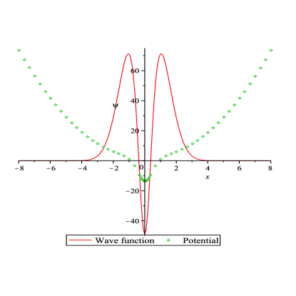
For example, implies, using (31), that , and thus we have for
| (34) |
the exact solution
with a plot of the wave function and potential given in Figure 1.
Further, , Eq.(31) implies
and we have for
| (35) |
the exact solutions
Similar results can be obtained for for .
II.3 Exactly solvable quantum isotonic nonlinear oscillator
As mentioned above, for and , it clear that for all and the one-dimensional Schrödinger equation
| (36) |
has the exact solutions
| (37) |
where are the polynomial solutions of the following second-order linear differential equation ()
| (38) |
By using AIM (Theorem 2, Eq.(21)), we find that the polynomial solutions of Eq.(38) are given explicitly as
| (39) |
a set of polynomial solutions that can be generated using
| (40) |
up to a constant factor, where, again, refers to the confluent hypergeometric function defined by (20). Note that the polynomials in equation (40) can be expressed in terms of the associated Laguerre polynomials temme as
| (41) |
III Quasi-polynomial solutions of the generalized quantum isotonic oscillator
In this section we study the quasi-polynomial solutions of the differential equation (II). We note first, using the change of variable , Eq.(II) can be written as
| (42) |
By means of the Möbius transformation that maps the singular points into , we obtain
| (43) |
where we assume
| (44) |
The differential equation (43) can be written as
| (45) |
which we may now compare with equation (14) in Theorem 1 with We, thus, conclude that the quasi-polynomial solutions of Eq.(III) are subject to the following conditions:
| (46) |
along with the vanishing of the tridiagonal determinant
= 0
where
| (52) |
Here, again, is fixed for given , the fixed size of the determinant .
III.1 Particular Case:
For , the differential equation (III) has the exact solution if and satisfies, simultaneously, the following system of equations
Solving this system of equations for and , we obtain the following values of
| (53) |
and the ground-state energy, in this case, is given by Eq.(44), namely,
| (54) |
which in complete agreement with the results of Section II.B.
III.2 Particular Case:
For , the determinant of (52) yields
| (58) |
where the energy is given by use of Eq.(44), for the computed values of and , by
| (59) |
Further, Eq.(58) yields the solutions for as functions of and
| (60) |
where the energy states are now given by (59) along with given by Eq.(60). We may also note that for
| (61) |
and
| (62) |
Further, for , we obtain the un-normalized wave function (see Eq.(8))
| (63) |
Thus, we may summarize these results as follows. The exact solutions of the Schrödinger equation (7) are given by Eqs.(62) and (63) only if and are the solutions of the system given by Eq.(58). In Tables 1 and 2, we report few quasi-exact solutions that can be obtained using this approach.
| Conditions | ||||
|---|---|---|---|---|
| 1 | ||||
| 0 | ||||
| Conditions | ||||
|---|---|---|---|---|
| 0 | ||||
III.3 Particular Case
For , the determinant along with the necessary condition (52) yields
| (64) |
where, again, the energy is given, for the computed values of and using Eqs.(44) and (64), by
In Table 3, we report the numerical results for some of the exact solutions of and using Eq. (64) and the values of , , , , and respectively. We have also computed the corresponding eigenvalues .
| Conditions | ||||
|---|---|---|---|---|
IV Numerical computation by use of the asymptotic iteration method
For the potential parameters and , not necessarily obeying the conditions for quasi-polynomial solutions discussed in the previous sections, the asymptotic iteration method can be employed to compute the eigenvalues of Schrödinger equation (7) for arbitrary values and . The functions and , using Eqs.(43) and (44), are given by
| (65) |
where . The AIM sequence and can be calculated iteratively using the iterative sequences (II.1). The energy eigenvalues of the quantum nonlinear isotonic potential (7) are obtained from the roots of the termination condition (22). According to the asymptotic iteration method, in particular the study of Brodie et al brodie , unless the differential equation is exactly solvable, the termination condition (22) produces for each iteration an expression that depends on both and (for given values of the parameters , and ). In such a case, one faces the problem of finding the best possible starting value that stabilizes the AIM process brodie . Fortunately, since , the starting value doesn’t represent a serious issue in our eigenvalue calculation using (65) and the termination condition (22) in contrast to the case of computing the eigenvalues using and as given by, for example, equation (II), where . In Table 4, we report our numerical results for energies of the four lowest states of the generalized isotonic oscillator of parameters and such that and for different values of . In this table, we set for computing the energies and , while we put for computing the energies and , respectively. For most of these values, the starting value of is and is shifted towards zero as gets larger in value. For the values of that admit a quasi-polynomial solution, the number of iteration doesn’t exceed three. For most of the other values of , the total number of iteration didn’t exceed 65. We found that for and the values of reported in Table 4, the number of iteration is relatively small compared to the case of and a large value of the parameter . The numerical computations in the present work were done using Maple version 13 running on an IBM architecture personal computer in a high-precision environment. In order to accelerate our computation we have written our own code for a root-finding algorithm instead of using the default procedure Solve of Maple 13. These numerical results are accurate to the number of decimals reported.
V Conclusion
We have provided a detailed solution of the eigenproblem posed by Schrödiger’s equation with a generalized nonlinear isotonic oscillator potential. We have presented a method for computing the quasi-polynomial solutions in cases where the potential parameters satisfy certain conditions. In other more general cases we have used the asymptotic iteration method to find accurate numerical solutions for arbitrary values of the potential parameters , and .
Acknowledgments
Partial financial support of this work under Grant Nos. GP249507 and GP3438 from the Natural Sciences and Engineering Research Council of Canada is gratefully acknowledged by two of us (respectively NS and RLH).
References
- (1) J. F. Cariñena, A. M. Perelomov, M. F. Rańada and M. Santander, A quantum exactly solvable nonlinear oscillator related to the isotonic oscillator, J. Phys. A: Math. Theor. 41 (2008) 085301.
- (2) B. Champion, R. L. Hall, and N. Saad, Asymptotic Iteration Method for singular potentials, Int. J. Mod. Phys. A 23 (2008) 1405 - 1415.
- (3) H. Ciftci, R. L. Hall, N. Saad, and E. Dogu, Physical applications of second-order linear differential equations that admit polynomial solutions, J. Phys. A: Math. Theor. 43 (2010) 415206.
- (4) H. Ciftci, R. L. Hall, and N. Saad, Asymptotic iteration method for eigenvalue problems, J. Phys. A: Math. Gen. 36 (2003) 11807.
- (5) H. Ciftci, R. L. Hall, and N. Saad, Construction of exact solutions to eigenvalue problems by the asymptotic iteration method, J. Phys. A: Math. Gen. 38 (2005) 1147.
- (6) J. M. Fellows, R. A. Smith, Factorization solution of a family of quantum nonlinear oscillators, J. Phys. A: Math. Theor. 42 (2009) 335303.
- (7) R. L. Hall, N. Saad, and A. B. von Keviczky, Spiked harmonic oscillators, J. Math. Phys. 43 (2002) 94.
- (8) A. Ronveaux (ed.), Heun’s Differential Equations, Oxford University Press, New York (1995).
- (9) J. Sesma, The generalized quantum isotonic oscillator, J. Phys. A: Math. Theor. 43 (2010) 185303.
- (10) N. M. Temme, Special functions: an introduction to the classical functions of mathematical physics, Wiley, New York, (1996). Laguerre polynomials are discussed in chapter 6.