Simplest model to study reentrance in physical systems

Abstract

We numerically investigate the necessary ingredients for reentrant behavior in the phase diagram of physical systems. Studies on the possibly simplest model that exhibits reentrance, the two-dimensional random bond Ising model, show that reentrant behavior is generic whenever frustration is present in the model. For both discrete and continuous disorder distributions, the phase diagram in the disorder–temperature plane is found to be reentrant, where for some disorder strengths a paramagnetic phase exists at both high and low temperatures, but an ordered ferromagnetic phase exists for intermediate temperatures.

Reentrance in a thermodynamic phase diagram presents a counterintuitive scenario: one phase exists inside some closed temperature range, with transitions to the same second phase at both higher and lower temperatures. If one of these phases is more ordered than the other one, then one of the phase transitions must violate the intuition that lower temperature phases are more ordered than higher temperature phases. In the context of solid-liquid transitions, this is known as “inverse melting” or “inverse freezing.” A variety of materials have been shown to have reentrant phase diagrams. For example, Rochelle salt was found to be a ferroelectric with two Curie points; the ordered ferroelectric phase occurs only between these two temperatures Jona and Shirane (1962). More recently, similar phase diagrams have been seen for superconducting vortices Fertig et al. (1977); Avraham et al. (2001), liquid crystals Cladis (1975), miscibility in solutions Zaǐtsev et al. (1986), polymeric materials van Ruth and Rastogi (2004), ferromagnetism in semiconductors Krivoruchko et al. (2010), denaturation of DNA Hanke et al. (2008), and many other systems Cladis (1988); Schupper and Shnerb (2005).

Theoretically, a number of model systems have been found with reentrant phase diagrams. The Ising model on a Union Jack lattice with frustrated anisotropic interactions was shown to be reentrant in a narrow region of parameter space Vaks et al. (1966); Morita (1985). In the fully-frustrated Villain model Villain (1977) the ground state of the system is seen to be disordered, while the low-lying excited states favor ferromagnetic ordering; in this case the ordering is due to the emergence of ferrimagnetism Villain et al. (1980). Reentrant ferromagnetism has also been seen in models of semiconductors because the carrier density increases with temperature Petukhov et al. (2007); in models of solid hydrogen, reentrance is due to quantum fluctuations Hetényi et al. (1999). Most prominently, frustrated spin-glass models have been shown to include the complexity necessary to describe rather generic reentrant scenarios Berker and Walker (1981); Schupper and Shnerb (2004); Crisanti and Leuzzi (2005); Paoluzzi et al. (2010); Ferreira et al. (2010), albeit for models with complex Hamiltonians.

Here we show numerically that the two-dimensional random-bond Ising model (RBIM)—possibly the simplest disordered spin model with frustration—generically possesses reentrance in its phase diagram for both discrete and continuous disorder distributions. It is given by the Hamiltonian

$$\textstyle{\mathcal{H}=-\sum_{\langle ij\rangle}J_{ij}s_{i}s_{j}}$$ (1)

with an $L\times L$ square toroidal grid com of Ising spins $\{s_{i}\in\pm 1\}$ and quenched nearest-neighbor random couplings $J_{ij}$. These random couplings are most commonly chosen from either a bimodal ($\pm J$) or Gaussian distribution. We emphasize that this Hamiltonian is much simpler than the disordered spin models typically used to study inverse freezing (e.g., the “simplest” model of inverse freezing Crisanti and Leuzzi (2005)). Furthermore, the phase diagram of this model is uncomplicated. At any finite temperature, with a disorder distribution biased toward ferromagnetic interactions, only ferromagnetic and paramagnetic phases are possible Fisher and Huse (1988). Because reentrance scenarios often occur in complex phase diagrams with many distinct phases, such a clean example is difficult to find in reentrant models.

The random-bond Ising model.—

The RBIM is widely studied as a standard model of disordered systems; it is one of the simplest models which includes the disorder and frustration needed to exhibit a complex glassy behavior at low temperatures Binder and Young (1986). These same elements, especially frustration, are necessary for the reentrant behavior in the phase diagram seen here. Furthermore, the model and cousins on more complex lattice geometries are of paramount importance across disciplines and more recently have found widespread use in the computation of the error stability of topologically-protected quantum computing proposals Kitaev (2003); Dennis et al. (2002); Katzgraber et al. (2009). For quantum computing applications, the order-disorder transition corresponds to the maximum error rate at which quantum operations may be performed with high fidelity. This relation is particularly apparent because the quantity we use to identify the phase transition in the RBIM is closely related to the error rate in the quantum computing proposals.

We study the phase diagram for this model with both discrete and continuous bond disorder $\{J_{ij}\}$. For the discrete $\pm J$ distribution, bond values are chosen according to

$$P(J_{ij})=p\delta(J_{ij}-J)+(1-p)\delta(J_{ij}+J).$$ (2)

The pure Ising model is recovered for $p\to 1$, while the strong-disorder case is typically studied for $p=0.5$. The disorder strength $q=1-p$ gives the deviation from a pure ferromagnet, but note that the free energy $F$ of the model is symmetric under reflection about $p=0.5$, so $F(T,p)=F(T,q)$. Nishimori has shown that, due to extra symmetries of the problem, a number of quantities, such as the internal energy of the system, may be computed exactly when the equality $(1-p)/p=\exp(-2J/T)$ holds Nishimori (1981). This equality is called the Nishimori line. The location of the phase transition on the Nishimori line, $(T_{c}^{*},p_{c}^{*})$, has been identified with a multicritical point Le Doussal and Harris (1988). Of interest here is that the magnetization for a given value of $p$ must be greatest on the Nishimori line, so that the ferromagnetic phase must not exist at any temperature for $p<p_{c}^{*}$ Nishimori (1981). This implies that the phase diagram below the Nishimori line is either vertical or reentrant. It has been argued analytically that the vertical case is the correct one Kitatani (1992); Ozeki and Nishimori (1993), although numerical studies with $\pm J$ disorder suggest a reentrant phase diagram Nobre (2001); Wang et al. (2003); Amoruso and Hartmann (2004); Parisen Toldin et al. (2009).

For the Gaussian distribution, bonds are chosen from

$$P(J_{ij})=(2\pi\widetilde{J}^{2})^{-1/2}\exp\left[-(J_{ij}-J)^{2}/2\widetilde{J}^{2}\right].$$ (3)

The pure Ising model is recovered for $\widetilde{J}\to 0$, while the strong disorder case occurs when $\widetilde{J}=1$ and $J=0$. The free energy of the model is symmetric under reflection about $\widetilde{J}=0$. It is customary McMillan (1984); Melchert and Hartmann (2009) to define a disorder strength parameter $r=\widetilde{J}/J$. In the case of Gaussian disorder, the Nishimori line Nishimori (1981) is given by $\widetilde{J}^{2}/T=J$. Here, the multicritical point $(T_{c}^{*},r_{c}^{*})$ is also the largest value of $r$ for which a ferromagnetic phase may exist, so that the phase diagram for Gaussian disorder is also expected to be either vertical or reentrant.

Unfortunately, the exact location of the multicritical point has not been calculated for either disorder distribution; numerical estimates for $\pm J$ disorder have given values of $q_{c}^{*}=0.1094(2)$ Honecker et al. (2001), $0.1093(2)$ Merz and Chalker (2002), and $0.10917(3)$ Parisen Toldin et al. (2009), while estimates for Gaussian disorder include $r_{c}^{*}=0.97945(4)$ Picco et al. (2007) and $0.9811(3)$, where the latter number was quoted as $1/r_{c}^{*}=1.0193(3)$ de Queiroz (2009). Exact efficient ground state algorithms exist for studying this model at zero temperature Barahona (1982), although the use of such techniques is complicated because they typically do not handle degeneracy well. Nevertheless, the values obtained are in the vicinity of $q_{c}(T=0)=0.103$ Wang et al. (2003); Amoruso and Hartmann (2004) and $r_{c}(T=0)=0.970(2)$ Melchert and Hartmann (2009), and clearly are not consistent with the values at the multicritical point.

One could still imagine a scenario where the $T=0$ behavior is significantly different from all finite-temperature behaviors: this is the case for the strong-disorder region of the phase diagram, where the $T=0$ spin-glass “phase” does not exist at nonzero temperatures Fisher and Huse (1988). Low-but-finite-temperature simulations are typically quite difficult due to long equilibration times, and the difference between the numerical estimates is quite small, so few points in between have been probed. The numerical measurement of the location of the phase transition at finite temperatures below the Nishimori line Merz and Chalker (2002); Parisen Toldin et al. (2009) has required thorough finite-size scaling extrapolation. Nevertheless, computations of $p_{c}(T)$ for two points below the Nishimori line have shown intermediate results Parisen Toldin et al. (2009). Here, our more efficient technique allows us to see the reentrance far more clearly than in previous studies.

Simulation details.—

To investigate the disorder-temperature phase diagram, we numerically identify the parameters that give the ferromagnet-paramagnet phase transition using a Pfaffian technique. Because this phase transition is of second order, the magnetization, which is the natural order parameter, is continuous. Quantities such as the Binder ratio Binder (1981) have been developed to most precisely determine the location of a phase transition. Here, we use a different quantity, which is more easily computed when the partition function is directly available.

We start be defining an extended Hamiltonian (see Ref. Thomas and Middleton (2007)) where the boundary conditions are allowed to vary, with both periodic and antiperiodic cases being allowed. The extended Hamiltonian is given by $\mathcal{H}^{*}=-\sum_{\langle ij\rangle}J_{ij}s_{i}s_{j}\sigma_{ij}$, with $\sigma_{ij}=1$ except on one vertical column of horizontal bonds where $\sigma_{ij}=\sigma_{v}$ and one horizontal row of vertical bonds, where $\sigma_{ij}=\sigma_{h}$; the $\sigma_{h,v}=\pm 1$. Defining a configuration $\{\{s_{i}\},\sigma_{v},\sigma_{h}\}$ of the system now requires specifying the spin values as well as the boundary conditions. The partition function, $\mathcal{Z}=\sum_{\{s_{i}=\pm 1\}}\exp(-\mathcal{H}/T)$, may also be extended to $\mathcal{Z^{*}}=\sum_{\{s_{i}=\pm 1\},\sigma_{v}=\pm 1,\sigma_{h}=\pm 1}\exp(-\mathcal{H^{*}}/T)$. Using a Pfaffian technique, $\mathcal{Z^{*}}$ may be directly evaluated from the same computation that produces $\mathcal{Z}$ with no additional computational effort. In this extended system we can compute the probability ${\tencyr zh}$ that the boundary conditions are periodic in both directions, given by

$${\tencyr zh}=\mathcal{Z}/\mathcal{Z^{*}}.$$ (4)

When the boundary conditions in a direction are changed from periodic to antiperiodic a system-spanning domain wall of length scale $L$ is imposed across the system. In the ferromagnetic phase, a system-spanning domain wall is energetically unfavorable: the periodic-periodic case, $\sigma_{v}=\sigma_{h}=1$, has lower free energy by an amount proportional to $L$ and therefore ${\tencyr zh}=1$ as $L\to\infty$. In the paramagnetic phase, the boundary conditions do not significantly influence the thermodynamics of the system, and all four cases have equal weight, so that ${\tencyr zh}=1/4$ as $L\to\infty$. At the phase transition, ${\tencyr zh}$ approaches a constant independent of $L$ (up to finite-size corrections), i.e., ${\tencyr zh}\sim\tilde{Z}[L^{1/\nu}(T-T_{c})]$. This measure is somewhat more sensitive than the free energy of a system-spanning domain wall because it allows for system-spanning domain walls in either or both directions. Note also that $1-{\tencyr zh}$ is equivalent to the error rate discussed in Ref. Wang et al. (2003). Thus the method we introduce here can be applied generically to the study of topologically-protected quantum computing proposals.

We have computed ${\tencyr zh}$ to investigate the phase diagram of the random-bond Ising model using a Pfaffian technique. With periodic boundary conditions, one may exactly compute $\mathcal{Z}$ by summing the Pfaffians of four related Kasteleyn matrices Thomas and Middleton (2009). The partition function of a system of $N=L\times L$ spins may be computed in $\mathcal{O}(N^{3/2})$ operations, allowing for exact partition function evaluation in systems up to $L=512$. By choosing different signs for the terms in the sum, it is also possible, without computing any additional Pfaffians, to compute $\mathcal{Z}$ for all four boundary conditions Thomas and Middleton (2009). Thus by computing $\mathcal{Z}$, we obtain $\mathcal{Z^{*}}$, and therefore ${\tencyr zh}$ for no extra effort.

Results.—

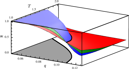
Figure 1: (Color online) Order probability ${\tencyr zh}$ as a function of temperature $T$ and disorder strength $q$ for the RBIM with $\pm J$ interactions for system sizes $L=16$, $32$, and $64$ (shallowest to steepest). Finite-size scaling corrections are small, i.e., the surfaces cross cleanly at the phase boundary (shown in the projection onto the plane). Error bars are smaller than the thickness of the surfaces.

Figure 1 shows the order probability ${\tencyr zh}$ as a function of temperature $T$ and disorder strength $q$ for the random-bond Ising model with $\pm J$ interactions and different system sizes. The data do cross at a line (see projection) that corresponds to the phase boundary, thus illustrating that the approach used works well. To extract the best estimate of the critical temperature $T_{c}$ for a given value of $q$ we perform a finite-size scaling of the data with $T_{c}$ and $\nu$ as free parameters. After performing a Levenberg-Marquard minimization of the chi² of the best fit to a third-order polynomial we estimate statistical errorbars by wrapping the process in a bootstrap analysis. The phase diagram for $\pm J$ disorder is shown in Fig. 2 and clearly shows reentrant behavior. We have these scaling collapses for data at fixed $q$ (squares) and $T$ (circles). To further highlight the reentrant behavior, in Fig. 3 we show the order probability as a function of temperature $T$ for $q=0.107$ (vertical line in Fig. 2). The data show two crossings, therefore clearly indicating that the phase diagram is paramagnet–ferromagnet–paramagnet with two distinct transitions.

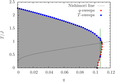
Figure 2: (Color online) Phase diagram of the two-dimensional random-bond Ising model with $\pm J$ interactions [Eq. (2)]. The shaded region is ferromagnetic, while the white region is paramagnetic. The boundary shown between these two regions is a guide to the eye. Some phase boundary points are computed by doing a scaling collapse varying $T$ (squares), while others are from a scaling collapse varying $q$ (circles). Statistical error bars which are smaller than the symbol size are not visible. For $q<0.05$, we use the results from Ref. Ohzeki et al. (2011), which used a related technique. The black circle for $q=0$ is the exact result for the pure Ising model. The point on the Nishimori line is from Ref. Parisen Toldin et al. (2009) and the $T=0$ point where the boundary touches the axis is from Ref. Amoruso and Hartmann (2004).

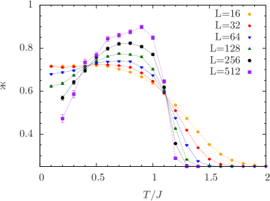
Figure 3: (Color online) Order probability $\tencyr zh$ as a function of temperature for $q=0.107$ (vertical line in Fig. 2) and $\pm J$ disorder. The data show two crossings, illustrating the existence of two transitions and therefore reentrance in the phase diagram.

Finally, in Figs. 4 and 5 we show data for Gaussian disorder. Reentrance is clearly present, albeit much weaker than for the $\pm J$ case: the ratio $r_{c}(T=0)/r_{c}^{*}\approx 0.99$ is much closer to $1$ than $q_{c}(T=0)/q_{c}^{*}\approx 0.94$ for the $\pm J$ case. These results show clearly that reentrance is a generic feature of this model when disorder and frustration are present. The fact that the case with Gaussian disorder has a much weaker effect suggests that the ground-state entropy might play a role but is not strictly necessary. In fact, studying a model where a continuous transition between the $\pm J$ and Gaussian cases can be tuned Pelikan et al. (2004) might help in elucidating this behavior, but it would be computationally extremely expensive. This tuning could change the magnitude of the reentrance, but it appears that the phase transitions are in the same universality class: the critical exponent $\nu$ is consistent with $\nu\approx 1.5$ for all points below the Nishimori line. For $\pm J$ disorder, we find an aggregate $\nu=1.49(4)$ while for Gaussian disorder, $\nu=1.52(5)$, in line with previous studies Wang et al. (2003); Amoruso and Hartmann (2004); Merz and Chalker (2002); Parisen Toldin et al. (2009); Melchert and Hartmann (2009); Picco et al. (2007); de Queiroz (2009).

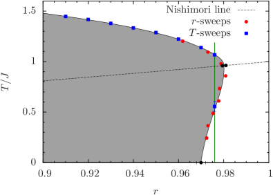
Figure 4: (Color online) Phase diagram of the two-dimensional random-bond Ising model with Gaussian disorder [Eq. (3)]. The shaded region is ferromagnetic, while the white region is paramagnetic. The black points on the Nishimori line are from Refs. Picco et al. (2007) (left) and de Queiroz (2009) (right), and the point at $T=0$ is from Ref. Melchert and Hartmann (2009). The boundary shown between these two regions is a guide to the eye.

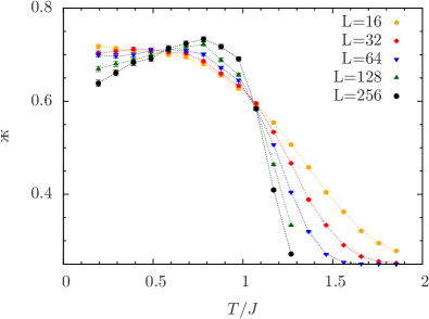
Figure 5: (Color online) Order probability $\tencyr zh$ as a function of temperature for $r=0.976$ (vertical line in Fig. 4) and Gaussian disorder. Although the approach to the thermodynamic limit is slow, the data clearly show two crossings, illustrating the existence of two transitions and therefore reentrance in the phase diagram.

Summary and Discussion.—

We have shown that the random-bond Ising model in two dimensions—a simply posed model with only two phases—generically possesses reentrance in its phase diagram. The disorder and frustration present in this model are responsible for this counterintuitive result. This is likely related to the “order by disorder” seen in the Villain fully frustrated model Villain et al. (1980). In the fully-frustrated case, ferromagnetic strips are completely decoupled from one another in the ground state, but the low-lying excitations have a weak ferromagnetic interaction among the strips. In the RBIM, the ground state consists of ferromagnetic domains of a size and energy scale set by the disorder strength. When these are dense enough to percolate throughout the system, ferromagnetic ordering will cease at $T=0$. However, for a range of parameters these domains can be coupled strongly enough in the low-lying excitations to produce the reentrant behavior in this model. It should be noted that the reentrance scenario shown here is particular to two space dimensions; the random bond Ising model in higher dimensions has a low-temperature spin glass phase so that if the ferromagnetic phase only exists for intermediate temperatures, the low-temperature phase would be a spin-glass phase and not the same paramagnetic phase found at high temperatures.