The spin-half Heisenberg antiferromagnet on two Archimedian lattices:
From the bounce lattice to the maple-leaf lattice and beyond

Abstract

We investigate the ground state of the two-dimensional Heisenberg antiferromagnet on two Archimedean lattices, namely, the maple-leaf and bounce lattices as well as a generalized $J$-$J^{\prime}$ model interpolating between both systems by varying $J^{\prime}/J$ from $J^{\prime}/J=0$ (bounce limit) to $J^{\prime}/J=1$ (maple-leaf limit) and beyond. We use the coupled cluster method to high orders of approximation and also exact diagonalization of finite-sized lattices to discuss the ground-state magnetic long-range order based on data for the ground-state energy, the magnetic order parameter, the spin-spin correlation functions as well as the pitch angle between neighboring spins. Our results indicate that the “pure” bounce ($J^{\prime}/J=0$) and maple-leaf ($J^{\prime}/J=1$) Heisenberg antiferromagnets are magnetically ordered, however, with a sublattice magnetization drastically reduced by frustration and quantum fluctuations. We found that magnetic long-range order is present in a wide parameter range $0\leq J^{\prime}/J\lesssim J^{\prime}_{c}/J$ and that the magnetic order parameter varies only weakly with $J^{\prime}/J$. At $J^{\prime}_{c}\approx 1.45J$ a direct first-order transition to a quantum orthogonal-dimer singlet ground state without magnetic long-range order takes place. The orthogonal-dimer state is the exact ground state in this large-$J^{\prime}$ regime, and so our model has similarities to the Shastry-Sutherland model. Finally, we use the exact diagonalization to investigate the magnetization curve. We a find a $1/3$ magnetization plateau for $J^{\prime}/J\gtrsim 1.07$ and another one at $2/3$ of saturation emerging only at large $J^{\prime}/J\gtrsim 3$.

I Introduction

The study of two-dimensional (2D) quantum spin-half antiferromagnetism is an interesting and challenging problem, in particular, if the magnetic interactions are frustrated. Man ; balents In 2D systems the interplay between geometry and quantum fluctuations may lead to semi-classical ground state (GS) phases with conventional magnetic long-range order (LRO) as well as to new quantum phases without magnetic LRO. Lhu ; wir04 The spin-$\frac{1}{2}$ Heisenberg antiferromagnet (HAF) on the eleven 2D Archimedian and related lattices presents an excellent opportunity to investigate the subtle balance of interactions and fluctuations and the role of lattice geometry. wir04 It is well-established that magnetic LRO is present in the GS of the spin-$\frac{1}{2}$ HAF on bipartite lattices (square Man ; wir04 , honeycombreger89 ; Mat ; wir04 , 1/5-depleted square (or CaVO) Tro ; Ma ; wir04 , square-hexagonal-dodecagonalToRi ; wir04 ). However, this magnetic order can be weakened or even suppressed by the presence of frustration. The first investigation of a frustrated quantum HAF goes back to the early 1970s, when Anderson and FazekasAnd ; Faz considered the spin-$\frac{1}{2}$ HAF on the triangular lattice. They conjectured a magnetically disordered GS. However, it is now clear that there is magnetic GS LRO in this system, see, e.g., Refs. Ber1, ; chub94, ; Cap, ; farnell01, ; wir04, ; farnell09, . The pioneering work of Anderson and Fazekas has formed the starting point for an intensive investigation of frustrated quantum magnetism. In particular, it has stimulated the search for non-magnetic quantum states in 2D magnetic systems.

Another well investigated frustrated 2D system is the HAF on the SrCuBO lattice, which can be transformed by an appropriate distortion to the Shastry-Sutherland square lattice modelShastry with equal strength of all exchange bonds. Again, the GS is magnetically long-range ordered, see e.g. Refs. Mila, ; hartmann00, ; koga00a, ; lauchli02, ; rachid05, . However, the magnetic LRO may be destroyed by a modification of bond strengths. Shastry ; Mila ; hartmann00 ; koga00a ; lauchli02 ; rachid05

The coordination number $z$ is quite large for the triangular ($z=6$) and SrCuBO ($z=5$ ) lattices, and that might be responsible for the semi-classical GS LRO found for the HAF on these frustrated Archimedian lattices. Thus, a “non-magnetic” quantum GS might be favored for lattices with lower coordination number $z$. Indeed, a regular depletion of the triangular lattice by a factor of 1/4 yields the Archimedian kagomé lattice with coordination number $z=4$. Contrary to the triangular lattice the GS of the spin-$\frac{1}{2}$ HAF on the kagomé lattice is most likely non-magnetic, see e.g. Refs. wir04, ; Lech, ; Wal, ; schmal_kag, ; singh07, ; white2010, . Another frustrated model with low coordination number $z=3$ having a non-magnetic quantum GS is the HAF on the Archimedian star lattice.wir04 ; star04 ; star07 ; star09 Moreover, we mention that the HAF on the (non-Archimedian) square-kagomé lattice with $z=4$ has most likely also a non-magnetic quantum GS.Sidd ; tomczak03 ; sp04 ; squago The above-mentioned depletion of the triangular lattice by a quarter is clearly not the only possibility. As has been pointed out by D. Betts Betts a regular depletion of the triangular lattice by a factor of 1/7 yields another translationally invariant lattice, namely the Archimedian maple-leaf lattice.Schmalfuss ; wir04 The coordination number of this lattice is $z=5$ and lies between those of the triangular ($z=6$) and the kagomé ($z=4$) lattices. Moreover, there is a frustrated Archimedian lattice with $z=4$, the so-called bounce lattice.wir04 Both the maple-leaf and the bounce lattices might be candidates for non-magnetic GSs. However, there are indications from previous studies (based on exact diagonalizations of finite-sized lattices) of semi-classical GS magnetic LRO Schmalfuss ; wir04 in the spin-$\frac{1}{2}$ HAF on these lattices. This conclusion was drawn based on only two finite lattices of $N=18$ and $N=36$ sites and therefore the conviction in the conclusions is lessened.

It is interesting to point out that the discussion of the magnetic properties of the HAF on Archimedian lattices is not only a challenging theoretical problem of quantum many-body physics but that it is also strongly relevant to experiment. Indeed, most of these lattices are found to be underlying lattice structures of the magnetic ions of various magnetic compounds, such as CaV₄O₉Tan , SrCu₂(BO₃)₂Kag , or [Fe₃($\mu_{3}$-O)($\mu$T-OAc)₆-(H₂O)₃][Fe₃($\mu_{3}$-O)($\mu$-OAc)_7.5]${}_{2}\cdot$7 H₂O.star Recently there has been also synthesized the magnetic compound $\mathrm{M_{x}}[\mathrm{Fe}(\mathrm{O}_{2}\mathrm{CCH}_{2})_{2}\mathrm{NCH}_{2}\mathrm{PO}_{3}]_{6}\cdot\mathrm{nH}_{2}\mathrm{O}$ (Ref. cave, ) with maple-leaf lattice structure as well as hybrid cobalt hydroxide materialsprice2011 with maple-leaf like lattice structure which may stimulate increasing interest in this lattice. Moreover, in the natural mineral spangolite (Cu₆Al(SO₄)(OH)₁₂Cl$\cdot$3H₂0) the magnetic copper ions sit on the lattice sites of the maple-leaf lattice.spango1 ; fennell In particular, spangolite is a very interesting magnetic system, since magnetic copper ions carry spin $1/2$ and the experimental data indicate that strong fluctuations at low temperatures are present which may prevent magnetic ordering.fennell In Ref. fennell, Fennell et al. propose that the spin-half Heisenberg model on the maple-leaf lattice with five different exchange integrals is the relevant model for this material.

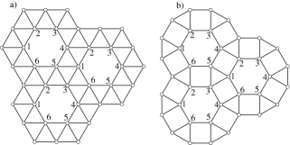
Figure 1: Archimedian Lattices: (a) 1/7-depleted triangular (maple-leaf) lattice. (b) bounce lattice. The six equivalent sublattices for both lattices are indicated by ‘1’, ‘2’, ‘3’, ‘4’, ‘5’, ‘6’

In this article we will discuss the GS properties of the spin-$\frac{1}{2}$ HAF on the maple-leaf and the bounce lattices, see Fig.1. These lattices are related to each other because the bounce lattice is equivalent to a bond-depleted maple-leaf lattice, see Ref. wir04, and Fig. 2. Therefore we will consider a generalized spin-$\frac{1}{2}$ $J$-$J^{\prime}$ HAF

$$H = J\sum_{\langle ij\rangle}{\bf s}_{i}\cdot{\bf s}_{j}+J^{\prime}\sum_{[ij]}{\bf s}_{i}\cdot{\bf s}_{j}\;;\;J>0\;;\;J^{\prime}\geq 0\;,$$ (1)

where ${\langle ij\rangle}$ runs over all nearest-neighbor (NN) bonds of the bounce lattice, and ${[ij]}$ runs over all additional NN bonds present in the maple-leaf lattice, cf. Figs. 2 and 3.

Figure 2: Illustration of the classical GS of $J-J^{\prime}$ model (Eq. (1); $J$ – solid lines; $J^{\prime}$ – dashed lines). The numbers 1, 2, 3, 4, 5, and 6 denote the six sites in the geometrical unit cell. The magnetic unit cell contains three geometrical unit cells $A$, $B$ and $C$.

A well-established method that can deal effectively with the GS properties of infinite 2D quantum magnets is given by the coupled cluster method (CCM) (see, e.g., Refs. Bi:1998_b, ; zeng98, ; bishop00, ; farnell04, ; ijmp2007, and references cited therein). The accuracy and effectiveness of this method in relation to the investigation of frustrated quantum spin systems has been strongly improved by the implementation of a parallelized CCM code cccm that carries out high-order CCM calculations. In particular, quantum phase transitions in 2D quantum spin systems that are driven by frustration can be studied by this method.krueger00 ; krueger01 ; rachid05 ; Schm:2006 ; bishop08 ; bishop08a ; rachid08 ; bishop09 ; richter10

II The classical ground state

We start with a brief illustration of the classical GS of the model (see Fig. 2) i.e. the ${\bf s}_{i}$ are treated as classical vectors of length $s$. The classical GSs in the limits $J^{\prime}=1$ and $J^{\prime}=0$ have already been discussed in Ref. wir04, . Starting from the information on the classical GS provided there it can be found easily for the $J-J^{\prime}$ model. The geometrical unit unit cell (hexagon) contains 6 sites labeled by the running index $n=1,...,6$. The magnetic unit cell is three times larger. Within one geometrical unit cell the pitch angle $\alpha$ between neighboring spins (e.g. spin on sites 1 and 2) around the hexagon is given by $\alpha=\pi-\arctan(\frac{J^{\prime}\sqrt{3}}{4J-J^{\prime}})$. Next-nearest neighbor spins on a hexagon (e.g. spins on sites 1 and 3) are parallel. Equivalent spins in two neighboring unit cells are rotated by a fixed angle $\pm 2\pi/3$, see the spin directions in unit cells $A$, $B$, $C$ shown in Fig. 2. In the limits $J^{\prime}=0$ (bounce lattice), $J^{\prime}=1$ (maple-leaf lattice) or $J^{\prime}\to\infty$ one has $\alpha=\pi$ and $E=-3JNs^{2}/2$, $\;\alpha=5\pi/6$ and $E=-(1+\sqrt{3})JNs^{2}/2$ or $\;\alpha\to\pi/3$ and $E\to-J^{\prime}Ns^{2}/2$, respectively.

III The Methods

III.1 Coupled Cluster Method (CCM)

We start with a brief illustration of the main features of the CCM. For a general overview on the CCM the interested reader is referred, e.g., to Refs. bishop91a, ; zeng98, ; farnell04, and for details of the CCM computational algorithm for quantum spin systems (with spin quantum number $s=1/2$) to Refs. zeng98, ; bishop00, ; krueger00, ; ijmp2007, . The starting point for a CCM calculation is the choice of a normalized model or reference state $|\Phi\rangle$, together with a set of mutually commuting multispin creation operators $C_{I}^{+}$ which are defined over a complete set of many-body configurations $I$. The operators $C_{I}$ are the multispin destruction operators and are defined to be the Hermitian adjoint of the $C_{I}^{+}$. We choose $\{|\Phi\rangle;C_{I}^{+}\}$ in such a way that we have $\langle\Phi|C_{I}^{+}=0=C_{I}|\Phi\rangle$, $\forall I\neq 0$. Note that the CCM formalism corresponds to the thermodynamic limit $N\rightarrow\infty$.

For spin systems, an appropriate choice for the CCM model state $|\Phi\rangle$ is often a classical spin state, in which the most general situation is one in which each spin can point in an arbitrary direction. We then perform a local coordinate transformation such that all spins are aligned in negative $z$-direction in the new coordinate frame.krueger00 ; krueger01 ; rachid05 As a result we have

$$|\Phi\rangle=|\downarrow\downarrow\downarrow\cdots\rangle;\quad C_{I}^{+}=s_{i}^{+},\,\,s_{i}^{+}s_{j}^{+},\,\,s_{i}^{+}s_{j}^{+}s_{k}^{+},\cdots,$$ (2)

(where the indices $i,j,k,\dots\;$ denote arbitrary lattice sites) for the model state and the multispin creation operators which now consist of spin-raising operators only.

The CCM parameterizations of the ket and bra ground states are given by

$$H|\Psi\rangle=E|\Psi\rangle\,\,;\qquad\langle\tilde{\Psi}|H=E\langle\tilde{\Psi}|\;\;;$$

$$|\Psi\rangle=e^{S}|\Phi\rangle\,\,;\qquad S=\sum_{I\neq 0}{\cal S}_{I}C_{I}^{+}\;\;;$$

$$\langle\tilde{\Psi}|=\langle\Phi|\tilde{S}e^{-S}\,\,;\qquad\tilde{S}=1+\sum_{I\neq 0}\tilde{\cal S}_{I}C_{I}^{-}\;.$$ (3)

The correlation operators $S$ and $\tilde{S}$ contain the correlation coefficients ${\cal S}_{I}$ and $\tilde{\cal S}_{I}$ that we must determine. Using the Schrödinger equation, $H|\Psi\rangle=E|\Psi\rangle$, we can now write the GS energy as $E=\langle\Phi|e^{-S}He^{S}|\Phi\rangle$ and the magnetic order parameter (sublattice magnetization) is given by $M_{s}=-\frac{1}{N}\sum_{i}^{N}\langle\tilde{\Psi}|s_{i}^{z}|\Psi\rangle$, where $s_{i}^{z}$ is expressed in the transformed coordinate system. (Note that all magnetic sublattices carry the same sublattice magnetization.)

To find the ket-state and bra-state correlation coefficients we require that the expectation value $\bar{H}=\langle\tilde{\Psi}|H|\Psi\rangle$ is a minimum with respect to the bra-state and ket-state correlation coefficients, such that the CCM ket- and bra-state equations are given by

$$\langle\Phi|C_{I}^{-}e^{-S}He^{S}|\Phi\rangle=0\qquad\forall I\neq 0$$ (4)

$$\langle\Phi|\tilde{\cal S}e^{-S}[H,C_{I}^{+}]e^{S}|\Phi\rangle=0\qquad\forall I\neq 0.$$ (5)

The problem of determining the CCM equations now becomes a pattern-matching exercise of the $\{C_{I}^{-}\}$ to the terms in $e^{-S}He^{S}$ in Eq. (4).

The CCM formalism is exact if we take into account all possible multispin configurations in the correlation operators $S$ and $\tilde{S}$. This is, however, generally not possible for quantum many-body models including that studied here. We must therefore use the most common approximation scheme to truncate the expansion of $S$ and $\tilde{S}$ in the Eqs. (4) and (5), namely the LSUB$n$ scheme, where we include only $n$ or fewer correlated spins in all configurations (or lattice animals in the language of graph theory) which span a range of no more than $n$ adjacent (contiguous) lattice sites (for more details see Refs. bishop91a, ; bishop00, ; krueger00, ; ijmp2007, ). For instance, one includes multispin creation operators of one, two, three or four spins distributed on arbitrary clusters of four contiguous lattice sites for the LSUB4 approximation. The number of these fundamental configurations can be reduced exploiting lattice symmetries. In the CCM-LSUB8 approximation we have finally $330369$ fundamental configurations.

Since the LSUB$n$ approximation becomes exact for $n\to\infty$, it is useful to extrapolate the ‘raw’ LSUB$n$ data in the limit $n\to\infty$. An appropriate extrapolation rule for the order parameter of systems showing GS magnetic LRO is given by $M_{s}(n)=a_{0}+a_{1}(1/n)+a_{2}(1/n^{2})$ (see, e.g., Refs. bishop00, ; farnell04, ; ijmp2007, ) where the results of the LSUB2,4,6,8 approximations are used for the extrapolation. For the GS energy per spin, $E(n)/N=b_{0}+b_{1}(1/n^{2})+b_{2}(1/n^{4})$ is a well-tested extrapolation ansatz.bishop00 ; krueger00 ; krueger01 ; farnell04 ; ijmp2007

III.2 Exact diagonalization (ED)

The Lanczos ED is a well-established many-body method, see, e.g., Ref. poilblanc, . Hence we can restrict our discussion of the method to some specific features relevant for our problem. The ED has been successfully applied to 2D frustrated quantum spin systems, see e.g. Refs. wir04, ; Wal, ; schulz, ; ED40, . Here we follow the lines of Ref. wir04, . For the system under consideration there are only two appropriate finite lattices, namely one with $N=18$ (see, Fig. 2 of Ref. Schmalfuss, ) and another one with $N=36$ (see Fig. 3). Note that these finite lattices do not have the the full lattice symmetry of the infinite lattice. Moreover the unit cell of these lattices is fairly large, namely it contains six sites. Hence, we consider the ED data as a complementary information to confirm or to question the CCM results corresponding to the thermodynamic limit $N\rightarrow\infty$. For the finite-size order parameter we usewir04

$$m^{+}=\sqrt{\frac{(M^{+})^{2}}{N^{2}}}=\left(\frac{1}{N^{2}}\sum_{i,j}^{N}{}|\langle{\bf s}_{i}{\bf s}_{j}\rangle|\right)^{1/2}\,.$$ (6)

We extrapolate the GS energy and the order parameter as described in Ref. wir04, (see also Refs. schulz, ; ED40, and references therein). However, the results of these ED extrapolations has to be taken with caution, since they are based only on two data points.

IV Results

Henceforth, we set $J=1$ and we consider $J^{\prime}$ as the active parameter in the model of Eq. (1). We apply high-order CCM up to LSUB8 and these infinite-lattice results are complemented by ED results of $N=18$ and $N=36$ sites, see Fig. 3. We choose the classical canted state illustrated in Sec. II to be the CCM reference or model state. As quantum fluctuations may lead to a “quantum” pitch angle that is different from the classical case, we consider the pitch angle $\alpha$ in the reference state as a free parameter. We then determine the quantum pitch angle $\alpha_{qu}$ by minimizing $E_{{\rm LSUB}n}(\alpha)$ with respect to $\alpha$ in each order $n$.

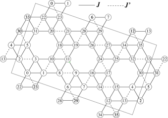
Figure 3: The finite maple-leaf lattice of 36 sites imposing periodic boundary conditions used for the ED calculations. Removing the dashed $J^{\prime}$ bonds the the exchange pattern corresponds to the bounce lattice of $N=36$ sites.

Table 1: CCM-results for the spin-$1/2$ HAFM on the bounce ($J^{\prime}=0$) and on the maple-leaf ($J^{\prime}=1$) lattices. $E/N$ is the GS energy per spin and $M_{s}$ is the sublattice magnetization. The LSUB$n$ results are extrapolated using $E(n)/N=b_{0}+b_{1}(1/n^{2})+b_{2}(1/n^{4})$ for the GS energy and $M_{s}(n)=a_{0}+a_{1}(1/n)+a_{2}(1/n^{2})$ for the sublattice magnetization.

bounce	$E/N$	$M_{s}$
LSUB2	-0.521631	0.404343
LSUB4	-0.546866	0.339357
LSUB6	-0.553763	0.298249
LSUB8	-0.556998	0.265252
Extrapolated CCM	-0.5605	0.1657
maple-leaf	$E/N$	$M_{s}$
LSUB2	-0.483470	0.405622
LSUB4	-0.512309	0.338483
LSUB6	-0.520378	0.297499
LSUB8	-0.523861	0.265768
Extrapolated CCM	-0.5279	0.1690

We start with the case of the perfect Archimedian bounce and maple-leaf lattices, and so we set $J^{\prime}=0$ and $J^{\prime}=1$, respectively. Results for the GS energy and sublattice magnetization are given for both lattices in Table 1. GS energies agree well with the previously reported data.wir04 ; Schmalfuss Furthermore, we confirm the previous findings that the GS is magnetically ordered. However, due to quantum fluctuations and frustration the sublattice magnetization is drastically reduced. Using our extrapolated CCM data (see Table 1) we find that the sublattice magnetizations are only $33\%$ of the classical value for the bounce lattice and $34\%$ of the classical value for the maple-leaf lattice. However, these values are still clearly above the ED estimates (which are $22\%$ for the maple-leaf and $27\%$ for the bounce lattice) of Ref. wir04, . We believe that the CCM data reported here are more reliable than the ED estimates because these ED results were extrapolated using only two data points ($N=18$ and $N=36$)misprint , see also Sec. III.2. These rather small values of the order parameter, which are significantly below that for the triangular lattice,Ber1 ; chub94 ; Cap ; farnell01 ; wir04 ; farnell09 indicate that the GS magnetic LRO is fragile, and one can speculate that slight modifications of the model parameters might lead to non-magnetic quantum GSs. We remark again that a related experimental material called spangolite fennell did not appear to shown magnetic LRO, and that this experimental result also spurs us on to evaluate the more general model.

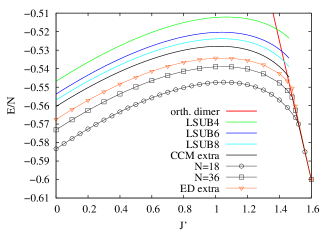
Figure 4: CCM results for the GS energy per spin $E/N$ as function of $J^{\prime}$. The CCM extrapolated values in the limit $n\to\infty$ are obtained using the extrapolation scheme $E(n)/N=b_{0}+b_{1}(1/n)^{2}+b_{2}(1/n)^{4}$. ED results for $N=18$ and $N=36$ as well as ED extrapolated values using the extrapolation scheme $E(N)/N=x_{0}+x_{1}N^{-3/2}$ are also shown. The red straight line shows the exact energy of the orthogonal-dimer state.

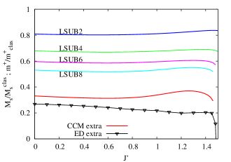
Figure 5: CCM results for magnetic order parameter (sublattice magnetization) $M_{s}$ as function of $J^{\prime}$. The data for the quantum model are scaled by its corresponding classical value $M_{s}^{clas}=1/2$. The extrapolated values in the limit $n\to\infty$ are found using the extrapolation scheme $M_{s}(n)=c_{0}+c_{1}(1/n)+c_{2}(1/n)^{2}$. We also show extrapolated finite-lattice results for the ED order parameter $m^{+}$ using the extrapolation scheme $m^{+}(N)=y_{0}+y_{1}N^{-1/2}$.

The results for the GS energy per spin are shown in Fig. 4 as a function of $J^{\prime}$. CCM LSUB$n$ results for the GS energy are clearly converging rapidly with increasing $n$ for all values of $J^{\prime}$. We have also used our ED data for $N=18$ and $N=36$ to extrapolate them to $N\to\infty$ (for the details of the extrapolation, see Ref. wir04, ). As already mentioned above this ED extrapolation has to be taken with caution, since it is based only on two data points. We find a reasonable agreement between the CCM and ED data for the GS energy. As indicated by the ED data the GS energy becomes linear in $J^{\prime}$ at larger $J^{\prime}\gtrsim 1.5$. This is related to the existence of a dimer product eigenstate where all $J^{\prime}$ bonds carry a dimer singlet.misguich99 We find that this singlet orthogonal-dimer eigenstate becomes the GS for $J^{\prime}>J^{\prime}_{c}$. Hence our model has much in common with the Shastry-Sutherland model Shastry ; Mila ; hartmann00 ; koga00a ; lauchli02 ; rachid05 that also demonstrates a similar exact orthogonal-dimer GS. We use the intersection point between the extrapolated CCM GS energy per site and the energy of the orthogonal-dimer eigenstate given by $E_{OD}/N=-3J^{\prime}/8$ to determine the transition point $J^{\prime}_{c}=1.449$. (Note that the corresponding value based on the ED data is $J^{\prime}_{c}=1.462$.)

Next we use the CCM results for the magnetic order parameter $M_{s}$ to discuss the stability of magnetic LRO as a function of $J^{\prime}$, see Fig. 5. It is obvious that the magnetic LRO persists in the whole region $0\leq J^{\prime}\leq J^{\prime}_{c}$. This conclusion is supported by the extrapolated ED order parameter also shown for comparison in Fig. 5. Interestingly the dependence of the order parameter on $J^{\prime}$ is fairly weak over the whole region $0\leq J^{\prime}\leq J^{\prime}_{c}$. Thus, the extrapolated CCM order parameter varies only between $29\%$ and $37\%$ of its classical value $M_{s}^{clas}=1/2$. This behavior might be interpreted as balanced interplay between increasing of frustration and increasing of the number of nearest neighbors when $J^{\prime}$ is growing. Our data for the order parameter lead to the conclusion that there is a direct first-order transition to the magnetically disordered orthogonal-dimer singlet GS.

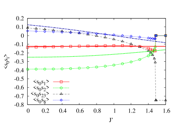
Figure 6: ED results for some selected spin-spin correlation functions $\langle{\bf s}_{0}{\bf s}_{i}\rangle$, $i=1,2,8,23$, for the finite lattice of $N=36$ sites shown in Fig. 3. The results for the quantum $s=1/2$ model are given by thin lines with symbols. The corresponding classical results are given by thick lines with the same color without symbols. The location of sites ’0’ and ’i’ in $\langle{\bf s}_{0}{\bf s}_{i}\rangle$ can be found in Fig. 3. Note that the classical curves for $\langle{\bf s}_{0}{\bf s}_{8}\rangle$ and $\langle{\bf s}_{0}{\bf s}_{23}\rangle$ coincide.

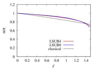
Figure 7: Results for the quantum pitch angle $\alpha_{qu}$ as a function of $J^{\prime}$ calculated within CCM-LSUB$n$ approximation with $n=4$ and $8$. The classical result $\alpha_{cl}$ is shown for the sake of comparison.

An additional confirmation of the above discussed behavior comes from the ED data for the spin-spin correlation functions $\langle{\bf s}_{i}{\bf s}_{j}\rangle$ presented in Fig. 6. Again we see that the variation of the correlation functions with $J^{\prime}$ is weak almost up to the transition point $J^{\prime}_{c}$. Moreover, for $J^{\prime}<J^{\prime}_{c}$ the correlation functions of the quantum model behave similar to those of the classical model.

Finally, in Fig. 7 we compare results for the classical pitch angle $\alpha_{cl}$, see Sec. II, and for the quantum pitch angle $\alpha_{qu}$ calculated by the CCM . We see that both $\alpha_{cl}$ and $\alpha_{qu}$ are close to each other and that there is only a slight variation of the pitch angle with $J^{\prime}$ (the value of the quantum pitch angle in CCM-LSUB8 approximation is $\alpha_{qu}=\pi$ at $J^{\prime}=0$, $\alpha_{qu}\approx 0.895\pi$ and it is still $\alpha_{qu}\approx 0.714\pi$ at $J^{\prime}=J^{\prime}_{c}$). Moreover, the LSUB4 and LSUB8 data for $\alpha_{qu}$ almost coincide.

Altogether, our data for the order parameter, the spin-spin correlation functions, and the pitch angle lead to the conclusion that there is most likely a direct first-order transition from a magnetically ordered state with spin orientations similar to those of the classical GS to the magnetically disordered orthogonal-dimer singlet GS.

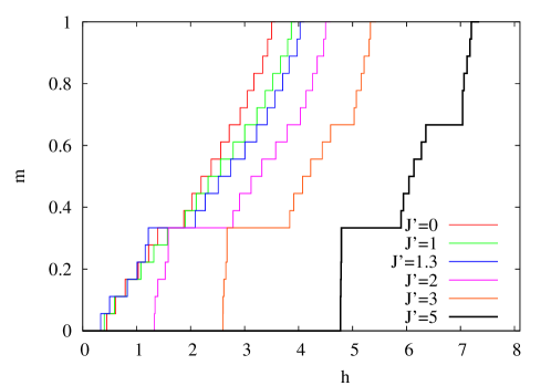
Figure 8: Results for the relative magnetization $m=M/M_{sat}$ versus applied field of strength $h$ obtained via ED for $N=36$, where $M_{sat}$ is the saturation magnetization.

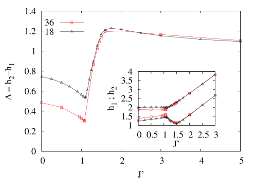
Figure 9: ED results ($N=18,36$) for the $m$=1/3 plateau. Main panel: Width $\Delta=h_{2}-h_{1}$ of the plateau versus $J^{\prime}$. Inset: End points $h_{1}$ and $h_{2}$ of the plateau versus $J^{\prime}$.

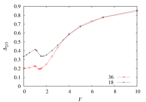
Figure 10: ED results ($N=18,36$) for the width of the m=2/3 plateau in dependence on $J^{\prime}$.

V Magnetization process

The magnetization process of frustrated quantum magnets has attracted much attention due to the discovery of exotic parts of the magnetization curve, such as plateaus and jumps, see e.g. Refs. nishi, ; Hon1999, ; LhuiMi, ; jump, ; HSR04, . The magnetization curves for the pure bounce ($J^{\prime}=0$) and maple-leaf ($J^{\prime}=1$) HAF were discussed already in Ref. wir04, based on ED data for $N=36$, where no indications for plateaus and jumps were found. On the other hand, we have already seen that the interpolating maple-leaf/bounce lattice AF model considered here for larger values of $J^{\prime}$ has much in common with the Shastry-Sutherland model. In particular, that both have at zero field a orthogonal-dimer singlet ground state. It is well known that the magnetization curve of the material SrCu₂(BO₃)₂ as well as that of the corresponding Shastry-Sutherland model possesses a series of plateaus, see e.g. Refs. wir04, ; Kage, ; kodama, ; misguich, ; infinite, ; mila, . Motivated by this we study in this section the magnetization curve $M(h)$ (where $M$ is the total magnetization and $h$ is the strength of the external magnetic field) for the interpolating maple-leaf/bounce lattice AF model using ED for $N=18$ and $N=36$ sites. ED results for the relative magnetization $m=M/M_{sat}$ versus magnetic field $h$ for $N=36$ sites are shown in Fig. 8. In accordance with previous resultswir04 we do not see indications for a plateau for $0<J^{\prime}\leq 1$. Moreover it is obvious, that the finite-size singlet-triplet gap determining the size of the first plateau at $m=0$ is small at $J^{\prime}=0$, $J^{\prime}=1$ and $J^{\prime}=1.3$. That corresponds to our finding of a magnetically ordered GS for these values of $J^{\prime}$, and therefore the $m=0$ plateau should disappear for $N\to\infty$. However, a finite $m=0$ plateau exists in that parameter region where the orthogonal-dimer singlet state is the zero-field GS, since this GS is gapped.

Similar as for the Shastry-Sutherland model there is a well-pronounced 1/3 plateau appearing at larger values of $J^{\prime}$. Interestingly, this plateau emerges already for values of $J^{\prime}$ below $J^{\prime}_{c}\approx 1.5$. In Fig. 9 we show the width of the 1/3 plateau versus $J^{\prime}$ (main panel) as well as the end points of the plateau (inset) for $N=18$ and $N=36$. We observe a significant change at $J^{\prime}=J^{\prime}_{p_{1/3}}\approx 1.07$. Below $J^{\prime}_{p_{1/3}}$ the typical finite-size behavior appears, i.e. the plateau width shrinks with system size $N$ and it vanishes at $N\to\infty$. By contrast, for $J^{\prime}>J^{\prime}_{p_{1/3}}$ there are almost no finite-size effects. The plateau width increases rapidly up to about $J^{\prime}\approx J^{\prime}_{c}$ and then it remains almost constant for $J^{\prime}\gtrsim J^{\prime}_{c}$, where the end points of the plateau grow linearly with $J^{\prime}$. Moreover, from Fig. 8 we find that for larger values of $J^{\prime}\gtrsim 2$ there is a jump-like transition between the $m=0$ and the $m=1/3$ plateaus.

As already mentioned above, for the Shastry-Sutherland model a series of plateaus was observed. For the model under consideration here we find indications for a second plateau at $m=2/3$, see Figs. 8 and 10. This plateau emerges only for quite large values of $J^{\prime}>J^{\prime}_{p_{2/3}}\approx 3$. Again we observe very weak finite-size effects of the plateau width for $J^{\prime}>J^{\prime}_{p_{2/3}}$ (Fig. 10). Furthermore, our ED data suggest an almost direct jump from the $m=2/3$ plateau to saturation $m=1$.

Finally we have to mention, that our finite-size analysis of the plateaus naturally could miss other plateaus present in infinite systems, see e.g. the discussion of the ED data of the $m(h)$ curve of the Shastry-Sutherland model in Ref. wir04, . Hence, the study of the magnetization process needs further attention based on alternative methods.

VI Conclusions

In this article we have treated a $J$-$J^{\prime}$ spin-half HAF interpolating between the HAF on the maple-leaf ($J^{\prime}=J$) and the bounce lattice ($J^{\prime}=0$). Moreover, we also discuss the GS for larger values $J^{\prime}>J$. This antiferromagnetic system is geometrically frustrated and it is related to several magnetic materials which have been experimentally investigated recently.cave ; price2011 ; fennell On the classical level the ground state is a commensurate non-collinear antiferromagnetic state. To study the quantum GS of the spin-half model we use the CCM for infinite lattices and the ED for finite lattices of $N=18$ and $N=36$ sites.

We find evidence for a semi-classical magnetically ordered commensurate non-collinear GS in a wide range of the exchange ratio $0\leq J^{\prime}/J\leq J^{\prime}_{c}/J\approx 1.5$. However, due to frustration and quantum fluctuations the sublattice magnetization amounts about $30\%$ of the classical value only. Importantly, we find that at $J^{\prime}_{c}\approx 1.45J$ there is a (most likely) first-order transition to a magnetically disordered orthogonal-dimer singlet product GS which is the exact GS for $J^{\prime}/J>J^{\prime}_{c}/J$. Therefore, the considered model is somewhat similar to the Shastry-Sutherland model. This similarity is also observed in the magnetization curve. Based on ED data we find evidence for plateaus at zero magnetization for $J^{\prime}/J>J^{\prime}_{c}/J$ (which is related to the gapped orthogonal-dimer singlet GS), at $1/3$ of saturation for $J^{\prime}\gtrsim 1.07J$ and at $2/3$ of saturation for $J^{\prime}\gtrsim 3J$. The transition to the $1/3$ plateau and from the $2/3$ plateau to saturation can be jump-like. Further plateaus not compatible to the system sizes $N=18$ and $N=36$ and therefore missed in the ED study may appear in the infinite system.

Our results may also stimulate other studies on this interesting 2D frustrated quantum system using other approximate methods to compare and contrast our results. In particular, the influence of modifications of the exchange bonds which might be relevant for real-life materials may lead to a destabilization of magnetic order. Knowing that the corresponding Shastry-Sutherland model exhibits a series of magnetization plateaus the search for further plateaus may be also an interesting problem to be studied by different means.

Acknowledgment For the exact digonalization J. Schulenburg’s spinpack was used. The authors are indebted to T. Fennell for providing information on spangolite prior to publication.

References

- (1) E. Manousakis, Rev. Mod. Phys. 63, 1 (1991).
- (2) L. Balents, Nature 464, 199 (2010).
- (3) G. Misguich and C. Lhuillier, in “Frustrated Spin Systems”, H. T. Diep, Ed. (World Scientific, Singapore, 2004), pp.229-306.
- (4) J. Richter, J. Schulenburg and A. Honecker, in Quantum Magnetism, eds U. Schollwöck, J. Richter, D.J.J. Farnell, and R.F. Bishop, Lecture Notes in Physics 645 (Springer-Verlag, Berlin, 2004), p. 85.
- (5) J.D. Reger, J.A. Riera, A.P. Young: J. Phys.: Condens. Matter 1, 1855 (1989)
- (6) A. Mattsson, P. Fröjdh, T. Einarsson, Phys. Rev. B 49, 3997 (1994).
- (7) M. Troyer, H. Kontani, K. Ueda, Phys. Rev. Lett. 76, 3822 (1996).
- (8) L.O. Manuel, M.I. Micheletti, A.E. Trumper, H.A. Ceccatto, Phys. Rev. B 58, 8490 (1998).
- (9) P. Tomczak and J. Richter, Phys. Rev. B 59, 107 (1999).
- (10) P.W. Anderson, Mater. Res. Bull. 8 153 (1973).
- (11) P. Fazekas and P.W. Anderson, Philos. Mag. 30, 423 (1974).
- (12) B. Bernu, C. Lhuillier, and L. Pierre, Phys. Rev. Lett. 69, 2590 (1992).
- (13) A. V. Chubukov, S. Sachdev, and T. Senthil, J. Phys.: Condens. Matter 6, 8891 (1994).
- (14) L. Capriotti, A.E. Trumper, and S. Sorella, Phys. Rev. Lett. 82, 3899 (1999).
- (15) D.J.J. Farnell, R.F. Bishop, and K.A. Gernoth: Phys. Rev. B 63, 220402(R) (2001)
- (16) D.J.J. Farnell, R. Zinke, J. Schulenburg, and J. Richter, J. Phys.: Condens. Matter 21, 406002 (2009).
- (17) B. S. Shastry and B. Sutherland, Physica B 108, 1069 (1981).
- (18) M. Albrecht and F. Mila, Europhys. Lett. 34, 145 (1996).
- (19) E. Müller-Hartmann, R.R.P. Singh, C. Knetter, and G.S. Uhrig, Phys. Rev. Lett. 84, 1808 (2000).
- (20) A. Koga and N. Kawakami, Phys. Rev. Lett. 84, 4461 (2000).
- (21) A. Läuchli, S. Wessel, and M. Sigrist, Phys. Rev. B 66, 014401 (2002).
- (22) R. Darradi, J. Richter, and D.J.J. Farnell, Phys. Rev. B 72, 104425 (2005).
- (23) P. Lecheminant, B. Bernu, C. Lhuillier, L. Pierre, and P. Sindzingre, Phys. Rev. B 56, 2521 (1997).
- (24) Ch. Waldtmann, H.U. Everts, B. Bernu, C. Lhuillier, P. Sindzingre, P. Lecheminant, and L. Pierre, Eur. Phys. J. B 2, 501 (1998).
- (25) D. Schmalfuß, J. Richter, and D. Ihle, Phys. Rev. B 70, 184412 (2004).
- (26) R.R.P. Singh and D. A. Huse, Phys. Rev. B 76, 180407(R) (2007).
- (27) S. Yan, D.A. Huse, and S.R. White, arXiv:1011.6114 (2010)
- (28) J. Richter, J. Schulenburg, A. Honecker, and D. Schmalfuß, Phys. Rev. B 70, 174454 (2004).
- (29) G. Misguich and P. Sindzingre, J. Phys.: Condens. Matter 19 145202 (2007).
- (30) T.-P. Choy and Y. B. Kim, Phys. Rev. B 80, 064404 (2009); B.-J. Yang, A. Paramekanti, and Y. B. Kim, Phys. Rev. B 81, 134418 (2010).
- (31) R. Siddharthan and A. Georges, Phys. Rev. B 65, 014417 (2002).
- (32) P. Tomczak and J. Richter, J. Phys. A: Math. Gen. 36, 5399 (2003).
- (33) J. Richter, O. Derzhko, and J. Schulenburg, Phys. Rev. Lett. 93, 107206 (2004).
- (34) J. Richter, J. Schulenburg, P. Tomczak, and D. Schmalfuß, Cond. Matter Phys. 12, 507 (2009).
- (35) D.D.Betts, Proc.N.S.Inst.Sci. 40, 95 (1995).
- (36) D. Schmalfuß, P. Tomczak, J. Schulenburg, and J. Richter, Phys. Rev. B 65, 224405 (2002)
- (37) S. Taniguchi, T. Nishikawa, Y. Yasui, Y. Kobayashi, M. Sato, T. Nishioka, M. Kontani and K. Sano, J. Phys. Soc. Jpn. 64, 2758 (1995).
- (38) H. Kageyama H. Kageyama, K. Yoshimura, R. Stern, N. V. Mushnikov, K. Onizuka, M. Kato, K. Kosuge, C. P. Slichter, T. Goto, and Y. Ueda, Phys. Rev. Lett. 82, 3168 (2000).
- (39) Y.-Z. Zheng, M.-L. Tong, W. Xue, W.-X. Zhang, X.-M. Chen, F. Grandjean, and G. J. Long, Angew. Chem. Int. Ed. 46, 6076 (2007).
- (40) D. Cave, F.C. Coomer, E. Molinos, H.H. Klauss, and P.T. Wood, Angew. Chem. Int. Ed. 45, 803 (2006).
- (41) T.D. Keene, M-E. Light, M.B. Hursthouse, and D.J. Price, Dalton Trans. 40, 2983 (2011)
- (42) F.C. Hawthorne, M. Kimata, and R.K. Eby, Am. Mineral. 78 649 (1993).
- (43) T. Fennell, J.O. Piatek, R.A. Stephenson, G.J. Nilsen and H.M. Ronnow, J. Phys.: Condens. Matter 23, 164201 (2011).
- (44) R.F. Bishop Microscopic Quantum Many-Body Theories and Their Applications ed J. Navarro and A. Polls Lecture Notes in Physics 510 (Berlin: Springer-Verlag) 1998.
- (45) C. Zeng, D.J.J. Farnell, and R.F. Bishop, J. Stat. Phys. 90, 327 (1998).
- (46) R.F. Bishop, D.J.J. Farnell, S.E. Krüger, J.B. Parkinson, J. Richter, J. Phys. Condens. Matter 12, 6877 (2000).
- (47) D.J.J. Farnell and R.F. Bishop, in Quantum Magnetism, eds. U. Schollwöck, J. Richter, D.J.J. and R.F. Bishop, Lecture Notes in Physics 645 (Springer-Verlag, Berlin, 2004), p. 307.
- (48) J. Richter, R. Darradi, R. Zinke, and R.F. Bishop, Int. J. Modern Phys. B 21, 2273 (2007).
- (49) For the numerical calculation we use the program package ’The crystallographic CCM’ (D.J.J. Farnell and J. Schulenburg).
- (50) S.E. Krüger, J. Richter, J. Schulenburg, D.J.J. Farnell, and R.F. Bishop, Phys. Rev. B 61, 14607 (2000).
- (51) S. E. Krüger and J. Richter, Phys. Rev. B 64, 024433 (2001).
- (52) D. Schmalfuß, R. Darradi, J. Richter, J. Schulenburg, and D. Ihle, Phys. Rev. Lett. 97, 157201 (2006).
- (53) R. F. Bishop, P. H. Y. Li, R. Darradi, and J. Richter, J. Phys.: Condens. Matter 20, 255251 (2008).
- (54) R.F. Bishop, P.H.Y. Li, R. Darradi, J. Schulenburg and J. Richter, Phys. Rev. B 78, 054412 (2008).
- (55) R. Darradi, O. Derzhko, R. Zinke, J. Schulenburg, S.E. Krüger and J. Richter, Phys. Rev. B 78, 214415 (2008).
- (56) R.F. Bishop, P.H.Y. Li, D.J.J. Farnell, and C.E. Campbell, Phys. Rev. B 79, 174405 (2009).
- (57) J. Richter, R. Darradi, J. Schulenburg, D.J.J. Farnell, and H. Rosner, Phys. Rev. B 81, 174429 (2010).
- (58) Note here that there is a misprint in Ref. wir04, concerning the extrapolated GS energy per bond of the mapel-leaf lattice. The correct value reads .
- (59) G. Misguich, C. Lhuillier, B. Bernu, and C. Waldtmann, Phys. Rev. B 60, 1064 (1999).
- (60) R.F. Bishop, J.B. Parkinson, and Y. Xian, Phys. Rev. B 43, R13782 (1991); Phys. Rev. B 44, 9425 (1991).
- (61) N. Laflorencie and D. Poilblanc, in Quantum Magnetism, eds U. Schollwöck, J. Richter, D.J.J. Farnell, and R.F. Bishop, Lecture Notes in Physics 645 (Springer-Verlag, Berlin, 2004), p. 227.
- (62) H.J. Schulz and T.A.L. Ziman, Europhys. Lett. 18, 355 (1992); H.J. Schulz, T.A.L. Ziman, and D. Poilblanc, J. Phys. I 6, 675 (1996).
- (63) J. Richter and J. Schulenburg, Eur. Phys. J. B 73, 117 (2010).
- (64) H. Nishimori and S. Miyashita, J. Phys. Soc. Japan 55, 4448 (1986).
- (65) A. Honecker, J. Phys.: Condens. Matter 11, 4697 (1999).
- (66) C. Lhuillier and G. Misguich, in High Magnetic Fields, Lecture Notes in Physics 595 eds. C. Berthier, L.P. Lévy, and G. Martinez (Springer, Berlin, 2002), p. 161.
- (67) J. Schulenburg, A. Honecker, J. Schnack, J. Richter, and H.-J. Schmidt, Phys. Rev. Lett. 88, 167207 (2002).
- (68) A. Honecker, J. Schulenburg, and J. Richter, J. Phys.: Condens. Matter 16, S749 (2004).
- (69) H. Kageyama , K. Yoshimura, R. Stern , N.V. Mushnikov, K. Onizuka, M. Kato, K. Kosuge, C.P. Slichter, T. Goto and Y. Ueda, Phys. Rev. Lett. 82, 3168 (1999)
- (70) K. Kodama, M. Takigawa, M. Horvatic, C. Berthier, H. Kageyama, Y. Ueda, S. Miyahara, F. Becca, F. Mila, Science 298, 395, (2002)
- (71) G. Misguich, Th. Jolicoeur, and S. M. Girvin, Phys. Rev. Lett. 87, 097203 (2001).
- (72) J. Schulenburg and J. Richter, Phys. Rev. B 65, 054420 (2002).
- (73) J. Dorier, K.P. Schmidt, and F. Mila, Phys. Rev. Lett. 101, 250402 (2008).
- (74) S. E. Sebastian, N. Harrison, P. Sengupta, C. D. Batista, S. Francoual, E. Palm, T. Murphy, N. Marcano, H. A. Dabkowska, B. D. Gaulin, PNAS 107, 6175 (2010).