Optical dropout galaxies lensed by the cluster A2667

Abstract

Context. We investigate the nature and the physical properties of ten $z$, $Y$ and $J-$dropout galaxies selected in the field of the lensing cluster A2667.

Aims. This cluster is part of our project aimed at obtaining deep photometry at $\sim$0.8-2.5 microns with ESO/VLT HAWK-I and FORS2 on a representative sample of lensing clusters extracted from our multi-wavelength combined surveys with SPITZER, HST, and Herschel. The goal is to identify a sample of redshift z$\sim$ 7-10 candidates accessible to detailed spectroscopic studies.

Methods. The selection function is the usual dropout technique based on deep $I$, $z$,$Y$, $J$, $H$ and $Ks$-band images (AB$\sim$26-27, 3$\sigma$), targeting $z\gtrsim$7.5 galaxy candidates. We also include IRAC data between 3.6 and 8 $\mu$m, and MIPS 24$\mu$m when available. In this paper we concentrate on the complete $Y$ and $J-$dropout sample among the sources detected with a high S/N ratio in both $H$ and $Ks$ bands, as well as the bright $z$-dropout sources fulfilling the color and magnitude selection criteria adopted by Capak et al. (2011). SED-fitting and photometric redshifts were used to further constrain the nature and the properties of these candidates.

Results. 10 photometric candidates are selected within the $\sim 7^{\prime}\times 7^{\prime}$ HAWK-I field of view ($\sim$ 33arcmin² of effective area once corrected for contamination and lensing dilution at $z\sim$7-10). All of them are detected in $H$ and $Ks$ bands in addition to $J$ and/or IRAC 3.6$\mu$m/4.5$\mu$m images, with $H_{AB}$ ranging from 23.4 to 25.2, and have modest magnification factors between 1.1 and 1.4. Although best-fit photometric redshifts are obtained at high-$z$ for all these candidates, the contamination by low-$z$ interlopers is expected to range between $\sim$50-75% based on previous studies, and on comparison with the blank-field WIRCAM Ultra-Deep Survey (WUDS). The same result is obtained when photometric redshifts are computed using a luminosity prior, allowing us to remove half of the original sample. Among the remaining galaxies, two additional sources could be identified as low-$z$ interlopers based on a detection at 24$\mu$m and on the HST $z_{850}$ band. These low-$z$ interlopers are not well described by current spectral templates given the large break, and cannot be easily identified based on broad-band photometry in the optical and near-IR domains alone. A good fit at z$\sim$1.7-3 is obtained at assuming a young stellar population together with a strong extinction. Given the estimated dust extinction and high SFRs, some of them could be also detected in the IR or sub-mm bands.

Conclusions. After correction for contaminants, the observed number counts at z$\gtrsim 7.5$ seem to be in agreement with expectations for an evolving LF, and inconsistent with a constant LF since $z\sim 4$. At least one and up to three candidates in this sample are expected to be genuine high-$z$, although spectroscopy is still needed to conclude.

1 Introduction

Considerable advances have been made during the last years in the exploration of the early Universe with the discovery of several z$\sim$6-7 galaxies close to the end of reionization epoch (e.g. Kneib et al. 2004, Stanway et al. 2004, Bouwens et al. 2004, 2008, 2009, 2010, Iye et al. 2006, Stark et al. 2007, Bradley et al. 2008, Zheng et al. 2009), whereas five-year WMAP results place the first building blocks at $z=11.0\pm 1.4$, suggesting that reionization was an extended process (Dunkley et al. 2009). For now, very few galaxies beyond z$\sim$6.5 are spectroscopically confirmed (Hu et al. 2002, Cuby et al. 2003, Kodaira et al. 2003, Taniguchi et al. 2005, Iye et al. 2006), and the samples beyond this limit are mainly supported by photometric considerations (Kneib et al. 2004, Bouwens et al. 2004, 2006, 2008, 2009, 2010; Richard et al. 2006, 2008; Bradley et al. 2008, Zheng et al. 2009, Castellano et al. 2010, Capak et al. 2011). Strong evolution has been found in the abundance of galaxies between z$\sim$7-8 and z$\sim$3-4 (e.g. Bouwens et al. 2008) based on photometrically-selected samples, the star-formation rate (SFR) density being much smaller at very high-z up to the limits of the present surveys, in particular towards the bright end of the Luminosity Function (LF). A similar evolutionary trend is observed in narrow-band surveys searching for Lyman-alpha emitters (e.g. Iye et al. 2006, Cuby et al. 2007, Hibon et al. 2010).

Lensing clusters of galaxies provide a unique and priviledged view of the high-redshift Universe. This technique, often referred to as “gravitational telescope”, was first proposed by Zwicky (1937). It has proven highly successful in identifying several of the most distant galaxies known today thanks to magnifications by typically 1-3 magnitudes (e.g. Ellis et al. 2001, Hu et al. 2002, Kneib et al. 2004, Bradley et al. 2008, Zheng et al. 2009).

Our project is based on the photometric pre-selection of high-z candidates in lensing clusters using the Lyman-break technique (LBGs, e.g. Steidel et al. 1995), which has been proved successful to identify star-forming objects up to z$\sim$ 6 (Bunker et al. 2004, Bouwens et al. 2004 to 2009), as well as photometric redshifts. The long term goal is to substantially increase the present sample of redshift z$\sim$ 7-12 galaxies, and to study their physical properties and the star-formation activity using a multi-wavelength approach.

This paper presents the first results of the short-term ongoing survey aimed at completing a deep photometric survey at $\sim$0.8-2.5 microns with HAWK-I at ESO/VLT on a representative sample of strong-lensing clusters at intermediate redshift, extracted from our multi-wavelength combined survey with SPITZER/IRAC+MIPS, HST (ACS/WFC3/NIC3), Herschel OT Key Program, and sub-mm coverage. Herschel data on this field have been recently obtained with PACS and SPIRE as part of the Herschel Lensing Survey (HLS, PI. E. Egami; see also Egami et al. 2010). These results and data will be described in a forthcoming paper. The presence of a strong lensing cluster within the large field-of-view of HAWK-I ($\sim 7^{\prime}\times 7^{\prime}$) is expected to optimize the global efficiency of the survey by combining in a single shot the benefit of gravitational magnification and a large effective surveyed volume (see also Maizy et al. 2010).

In this paper we concentrate on the complete sample of $Y$ and $J-$dropout sources selected in the field of the lensing cluster A2667 (Abell 2667, $\alpha$=23:51:39.35 $\delta$=$-$26:05:03.1 J2000, $z=0.23$). For comparison we also examine the bright $z$-dropout sources fulfilling the color and magnitude selection criteria adopted by Capak et al. (2011). All the candidates are selected to represent star-forming galaxies at $z\gtrsim 7.5$, and to be bright enough for spectroscopic follow up, although a large fraction of galaxies selected in this way could be low-$z$ contaminants. SED-fitting and photometric redshifts are used to further constrain the nature and the properties of these candidates. The results achieved on the luminosity functions in the $z\gtrsim 7.0$ redshift domain will be presented elsewhere.

In Sect. 2 we summarize the photometric observations and data reduction. We also describe the construction and analysis of photometric catalogs. The selection of different dropout candidates is presented in Sect. 3. The properties of the selected candidates, including spectral energy distributions (hereafter SEDs), SED-fitting results and photometric redshifts are detailed in Sect. 4, together with a discussion on the reliability of the different high-$z$ candidates when photometric redshifts include a luminosity prior. In Sect. 5 we discuss the global properties of this sample, in particular expected versus observed number counts. We compare our results with previous findings and we discuss on the nature of low-$z$ contaminants. Conclusions are given in Sect. 6. The concordance cosmology is adopted throughout this paper, with $\Omega_{\Lambda}=0.7$, $\Omega_{m}=0.3$ and $H_{0}=70\ km\ s^{-1}\ Mpc^{-1}$. All magnitudes are quoted in the AB system (Oke & Gunn 1983). Table  1 presents the conversion values between Vega and AB systems for our photometric dataset.

2 Observations and data analysis

2.1 Ground-based optical and near-IR imaging

The selection of high-z candidates is based on deep optical and near-IR imaging. A2667 was observed with HAWK-I in the near-infrared domain ($\sim$ 0.9 to 2.2 $\mu$m, covering the 4 bands $Y$, $J$, $H$, and $Ks$), and with FORS2 in $I$ and $z$ bands, between October and November 2008. Data reduction and processing included photometric calibration, bias subtraction, flat-fielding, sky subtraction, registration and combination of images using IRAF, closely following the general procedures described in Richard et al. (2006). Table 1 summarizes the properties of the photometric dataset used in this paper.

For the FORS2 data, we used a standard flat-field correction and combination of the individual frames with bad-pixel rejection. In addition to the $z$ band image matching the HAWK-I field (hereafter $z_{1}$), an older image of similar quality centered on the cD galaxy, obtained in June 2003 (71.A-0428, hereafter $z_{2}$) was also used to confirm the non-detection of high-$z$ candidates in the common area.

For HAWK-I data, we used the ESO pipeline to process and combine all individual images, refining the offsets between the different epochs of observations when producing the final stack. This procedure performs a 2-step sky subtraction, using masks to reject pixels located on bright objects, similar to the XDIMSUM package as described in Richard et al. (2006). The photometric calibration was checked against 2MASS stars present in the field of view, taking into account the relative flat-field normalisations between each one of the 4 HAWKI chips. Before combining, we applied individual weight values according to: $weight\propto(ZP\times var\times{s}^{2})^{-1}$ where individual zero-point $ZP$ and seeing $s$ values were obtained from the brightest unsaturated stars around the field, and pixel-to-pixel variance $var$ was derived through statistics within a small region free of objects.

Photometric zero-points were derived from LCO/Palomar NICMOS standard stars (Persson et al. 1998). The final accuracy of our photometric calibration has been checked by comparing the observed colors of cluster elliptical galaxies, measured on images matched to the worst seeing in our data (i.e. $\sim 0.9$″in the $z_{1}$ band), to match expectations based on the empirical SED template compiled by Coleman, Wu and Weedman (CWW, 1980). According to this check, we expect our final photometric catalog to be accurate to about 0.05 mags throughout the wavelength domain between $I$ and $Ks$.

All HAWK-I images were registered and matched to a common seeing using a simple gaussian convolution in order to derive magnitudes and colors, the worst case being the $J$ band image. Astrometric calibration was performed in a standard way (see e.g. Richard et al. 2006), reaching an absolute accuracy of $\sim 0.2$ ″ for a whole HAWK-I field of view. Images in $I$ and $z$ bands were registered to the HAWK-I images using standard IRAF procedures for rotation, magnification and resampling of the data. These images were mainly used to exclude well-detected low-$z$ interlopers.

All high-$z$ candidates are expected to be detected in the $H$ and $Ks$ bands and to be undetected in $I$ and $z$ bands. Therefore, the original $H$ and $Ks$ band images were combined together to create an $H+Ks$ detection image with excellent seeing quality ($\sim 0.47$″). Also the original unregistered images in $I$ and $z$ bands were used for the visual inspection of the Y-dropout candidates. Error bars and non-detection criteria were also determined on the original images (see below). Photometry for the $z$ and $Y$-dropout sample was also obtained with near-IR images matched to the worst seeing in our data in order to check for consistency of observed colors.

We used the $SExtractor$ package version 2.8 (Bertin & Arnouts 1996) for detection and photometry. Magnitudes were measured in all images with the $SExtractor$ “double-image” mode, using the $H+Ks$ detection image as a reference. Magnitudes were measured within different apertures ranging from 1 to 2 ″diameter, as well as MAG_AUTO magnitudes. We checked that colors derived with different choices of aperture and magnitude types are consistent with each other within the errors. Photometric errors were measured using the typical RMS in the pixel distribution of the original images (without any seeing matching or rescaling), within apertures of the same physical size as for flux measurements (either aperture or MAG_AUTO magnitudes). Photometric errors measured on the original images were also used to compute $3\sigma$ limiting magnitudes in each band, reported in Table 1. Errors in colors were derived from the corresponding magnitude errors added quadratically.

Completeness values for point-sources detected in the different bands were obtained through Monte-Carlo techniques. Artificial stars (i.e., seeing limited sources) were added at $\sim$700 different random locations on our images, and then extracted using the same parameters for detection and photometry as for astronomical sources. The seeing was measured on the original co-added images. The corresponding results are shown in Fig. 1 and Table 1.

2.2 Other imaging observations

In addition to the images used for high-z sample selection, SED analysis is also supported by additional data when available for the candidates, namely:

• Images of Abell 2667 were obtained in the 3.6, 4.5, 5.8 and 8.0$\mu$m bands as part of the GTO Lensing Cluster Survey (Program 83, PI. G. Rieke), using the Infrared Array Camera (IRAC; Fazio et al. 2004) onboard the Spitzer Space Telescope (Werner et al. 2004). In addition, deeper exposures were obtained at 3.6 and 4.5$\mu$m in August 2009 (Program 60034, PI. E. Egami). All these images were processed according to Egami et al. (2006). IRAC magnitudes were measured within a 2″ diameter aperture and corrected according to the Instrument Handbook (v.1.0, February 2010). The field of view is 5.2 ′$\times$ 5.2 ′.

• We also gathered 24$\mu$m images in this field obtained with MIPS (Rieke et al. 2004), processed as described by Rigby et al. (2008).

• A deep HST F850LP/ACS image is also available on the cluster core (8.8 ksec, PI. R. Ellis; see also Richard et al. 2008). Photometry in this band is refered as $z_{850}$ hereafter.

The properties of the complete photometric dataset used in this paper are summarized in Table 1. 3.6 and 4.5$\mu$m images refer to the most recent and better quality dataset.

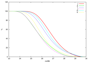
Figure 1: Completeness levels obtained from simulations for the different bands used for high-z sample selection: $I$ (solid red line), $z$ (dashed green line), $Y$ (dotted blue line), $J$ (dotted magenta line),$H$ (dot-dashed cyan line), and $Ks$ (dot-dashed yellow line).

Table 1: Photometric dataset: ground-based optical and near-IR imaging used in the selection of high-z candidates (top) and space-based complementary data (bottom)

Filter	$\lambda_{eff}$	$C_{AB}$	$t_{exp}$	pix	m(3$\sigma$)	m(50%)	seeing
	[nm]	[mag]	[ksec]	[″]	[mag]	[mag]	[″]
$I$	793	0.45	13.0	0.126	27.5	26.8	0.47
$z_{1}$	920	0.54	12.7	0.126	26.1	25.7	0.91
$z_{2}$	920	0.54	13.2	0.126	26.0	25.7	0.54
$Y$	1021	0.62	8.6	0.106	26.9	26.3	0.61
$J$	1260	0.95	9.2	0.106	26.3	25.7	0.64
$H$	1625	1.38	25.3	0.106	26.8	26.5	0.46
$Ks$	2152	1.86	11.0	0.106	25.9	25.8	0.47
						Ref.
$z_{850}$	9106	0.54	8.8	0.05	26.1	A
3.6$\mu$m	3575	2.79	16.8	1.2	25.1
4.5$\mu$m	4528	3.25	17.4	1.2	25.2
5.8$\mu$m	5693	3.70	2.4	1.2	22.7	B
8.0$\mu$m	7958	4.37	2.4	1.2	22.8	B
24$\mu$m	23843	6.69	2.7	2.55	18.7	C

Table 2: Catalogue of $z$, $Y$ and $J$-dropouts in A2667.

Source	RA	Dec	$H$	$\Delta H$	Stell.	FWHM	$\mu$	$\mu$	$\Delta\mu$	Q1	Q2	Q3	Q	$\chi^{2}_{opt}$	Final
	(J2000)	(J2000)				[″]	high-$z$	low-$z$
z1	23:51:45.837	-26:7:07.20	23.59	0.03	0.03	0.74	1.169	1.119	0.018	3	3	1	7-I	-0.03	(low)
Y1	23:52:00.157	-26:8:30.31	23.35	0.03	0.03	0.95	1.028	1.012	0.003	1	1	2	4-III	1.00	low
Y2	23:51:57.156	-26:4:02.37	23.45	0.03	0.40	0.58	1.108	1.031	0.007	2	2	1	5-III	1.19	low
Y3	23:51:43.332	-26:8:00.89	23.68	0.04	0.02	1.24	1.128	1.059	0.012	3	3	2	8-I	0.54	high
Y4	23:51:35.750	-26:7:10.65	23.80	0.04	0.12	0.74	1.371	1.111	0.020	1	3	2	6-II	0.64	high
Y5	23:51:54.448	-26:3:13.65	23.98	0.04	0.03	0.96	1.149	1.037	0.007	2	2	2	6-II	0.68	?
Y6	23:51:53.437	-26:4:29.94	24.37	0.08	0.02	1.81	1.167	1.067	0.011	1	1	3	5-III	0.07	low
Y7	23:51:56.568	-26:7:51.45	24.27	0.05	0.02	1.13	1.045	1.021	0.005	3	3	2	8-I	0.00	low
Y8	23:51:37.151	-26:2:30.46	25.40	0.08	0.97	0.46	1.183	1.140	0.018	1	2	3	6-II	0.58	low
J1	23:51:34.855	-26:3:32.74	25.21	0.08	0.97	0.55	1.299	1.398	0.033	3	3	2	8-I	0.60	(low)

Table 3: Photometric catalogue of bright $z$, $Y$ and $J$-dropouts in A2667.

Source	$I$	$z$	$Y$	$J$	$H$	$Ks$	3.6$\mu$m	4.5$\mu$m	5.8$\mu$m	8.0$\mu$m	24$\mu$m
z1(*)	$>$28.7	$>$27.2	25.63	23.29	23.59	23.00	21.79	21.38	-	21.41	17.57
			$\pm$0.15	$\pm$0.03	$\pm$0.03	$\pm$0.03	$\pm$0.01	$\pm$0.01		$\pm$0.10	$\pm$0.12
Y1	$>$28.7	-	27.04	24.08	23.35	22.73	-	-	-	-	-
			$\pm$0.35	$\pm$0.07	$\pm$0.03	$\pm$0.03
Y2	$>$28.7	$>$27.2	$>$28.1	24.17	23.45	22.81	-	21.80	-	-	-
				$\pm$0.15	$\pm$0.03	$\pm$0.03		$\pm$0.01
Y3(*)	$>$28.7	$>$27.2	25.51	23.85	23.68	23.07	22.84	22.52	-	-	$>$19.93
			$\pm$0.18	$\pm$0.07	$\pm$0.04	$\pm$0.04	$\pm$0.04	$\pm$0.03
Y4(*)	$>$28.7	26.42	$>$28.1	24.59	23.80	23.55	23.19	22.91	$>$23.93	$>$23.98	$>$19.93
		$\pm$0.50		$\pm$0.11	$\pm$0.04	$\pm$0.05	$\pm$0.06	$\pm$0.04
Y5(*)	$>$28.7	$>$27.2	$>$28.1	24.31	23.98	23.28	22.74	22.47	-	-	-
				$\pm$0.08	$\pm$0.04	$\pm$0.04	$\pm$0.04	$\pm$0.03
Y6(*)	$>$28.7	$>$27.2	26.91	24.84	24.37	23.75	-	-	-	-	-
			$\pm$0.33	$\pm$0.13	$\pm$0.08	$\pm$0.06
Y7	$>$28.7	$>$27.2	$>$28.1	25.22	24.27	23.75	22.53	22.68	-	-	18.78
				$\pm$0.12	$\pm$0.05	$\pm$0.08	$\pm$0.03	$\pm$0.03			$\pm$0.36
Y8(*)	$>$28.7	$>$27.2	26.86	25.58	25.40	25.08	-	-	21.24	22.12	$>$19.93
			$\pm$0.24	$\pm$0.30	$\pm$0.08	$\pm$0.12			$\pm$0.10	$\pm$0.19
J1(*)	27.39	$>$27.2	$>$28.1	$>$27.5	25.21	24.77	24.82	24.80	21.96	22.23	$>$19.93
	$\pm$0.49				$\pm$0.08	$\pm$0.11	$\pm$0.25	$\pm$0.22	$\pm$0.18	$\pm$0.21

3 Selection of high-$z$ galaxy candidates

The original catalog on the HAWK-I field of view includes $\sim 5\times 10^{4}$ objets over a $\sim$45 arcmin² area with more than 75% exposure time on the HAWK-I images. Since high-$z$ candidates should be detected both in the $H$ and $Ks$ bands, we first require a detection above 5$\sigma$ level in both filters within a 1.3″ diameter aperture. This means selecting sources with $H<$ 26.22 and $Ks<$ 25.43, corresponding to a completeness level in our survey of $\,\stackrel{{\scriptstyle>}}{{\scriptstyle\sim}}\,$70% for point sources (see Fig. 1). We also require less than a 2$\sigma$ level detection in both $I$ and $z$ bands. This selection yields a sample of 175 objects after removing all noisy areas on the $I$ and $z$ images, i.e. a common clean area of $\sim$42arcmin² (equivalent to $\sim$33arcmin² after correction for lensing dilution).

We then apply the following criteria to the remaining sample in order to select objects at $z>7$:

• $Y-J>0.8$, $J-H<1.2$, and $Y-J>1.25\times(J-H)+0.8$. This window, based on simulations using different spectral templates, selects $Y$-dropout $z\geq 7.3$ candidates. Fig. 2 displays the corresponding color-color diagram for different models, namely E-type galaxies (CWW), Im-type galaxies (constant star-formation model from Bruzual & Charlot 1993, 2003), and starburst templates of Kinney et al. (1996), together with the selection window. Other galaxy templates, such as the UV-to-radio spectral templates of galaxies and AGN from Polletta et al. (2007) used subsequently not shown here, populate a very similar area is this and other color-color plots. Also shown are the synthetic colors of cool stars (M, L, T types) from the SpexGrism spectral library (see Burgasser et al. 2006, and references therein) .

• $J-H>0.76$, $H-Ks<0.5$, and $J-H>1.3\times(H-Ks)+0.76$ illustrated in Fig. 3. Furthermore we require a non-detection in the $Y$ band, below the 2 $\sigma$ limit. This window is intended to select $J$-dropout candidates in the range $8\lesssim z\lesssim 10$ wich are well detected in $H$ and $Ks$ bands (cf. Richard et al. 2006). The corresponding color-color plot is shown in Fig. 3.

• The $z$-dropout selection criteria adopted by Capak et al. (2011) for their sample, i.e. $J<$ 23.7 (their 5$\sigma$ detection level), $z-J\geq 1.5$, $J-Ks>0$, and $Ks-4.5\mu m>0$ (cf. Fig. 4). The last criterium involving the $4.5\mu m$ band was not applied to our sample given the partial coverage of the HAWK-I field of view. Fig. 4 displays the corresponding color-color plot. This selection does in particular not make use of the $Y$ band filter, intermediate between $z$ and $J$, available for our observations.

There is some overlap between the $z$ and $Y$ bands, leading to somewhat ill-defined dropout criteria in $z-Y$. For this reason, we use instead $Y-J$ and $z-J$ in the above selection windows. Including the $Y$ band provides us with a useful discrimination between high-z galaxies and cool stars, as shown in Fig. 2, while improving photometric redshifts.

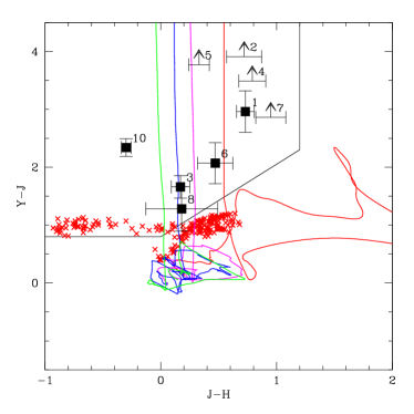
Figure 2: Color-color diagram showing the position expected for spectral templates with redshifts $z\sim$ 0–9.0: E-type galaxies (CWW; red solid line), Im-type galaxies (blue line), and starburst templates of Kinney et al. (1996) (magenta and green lines). Red crosses show the colors of M, L, T, stars from the SpeX Prism libraries of Burgasser et al. (2006). Black lines delimit our selection window for $z$ $\gtrsim$ 7.3 galaxies. Our 9 $Y-$dropout candidates are marked with black squares and arrows: # 1 to # 8 correspond to Y1 to Y8, whereas # 10 is z1.

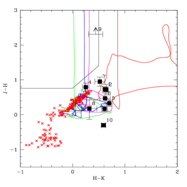
Figure 3: Same as Fig. 2 for (J-H) versus (H-K) colors showing one $J-$drop candidate (J1, #9) and the 9 $Y-$dropout candidates (same identifications as in Fig. 2).

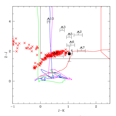
Figure 4: Same as Fig. 4 for (z-J) versus (J-K) colors. Thin black lines denote the selection window (c) (the same as in Capak et al. 2011). The same identifications as in Fig. 2 and Fig. 3 are used for the dropout candidates.

The blind selection windows (a) and (b) include 48 and 52 sources respectively (25 sources in common), i.e. 75 candidates in total out of the initial sample of 175 optical dropouts. Note that this selection does not introduce any restriction in magnitude except for the $\geq$5$\sigma$ level detection in $H$ and $Ks$. When applying the $z$-dropout selection criteria (c), 8 sources are found. All these optical dropouts were carefully examined by a visual inspection in the different (original) bands in order to reject both spurious detections in the near-IR images and false non-detections in the $I$ and $z$ bands. The main sources of contamination were images detected within the haloes of bright galaxies leading to fake measurements or highly contaminated photometry. A mask was created to remove these regions from the subsequent analysis (this corresponds to $\sim$15% of the total surface).

We have also checked that the selection based on the detection in $H$ and $Ks$ bands does not introduce a bias against intrinsically blue sources (see e.g. Finkelstein et al. 2010). The selection was repeated with the requirement of a detection above 5$\sigma$ in the $H$-band alone, all the other conditions for optical dropouts being the same. This new selection includes all the previous objects plus four additional sources, but none of them survived the manual inspection.

At the end of the visual inspection, only 10 candidates survive from the original sample. Their photometry is listed in Table 3. The brightest one in $J$ is the only source retained by selection criteria (c) after manual inspection (identified hereafter as z1). This source and 8 additional objects fulfill the $YJH$ color selection (a) (cf. Fig. 2), which closely follows the selection previously adopted by Bouwens et al. (2008) and Richard et al. (2008) in $zJH$. The latter 8 objects, denoted as Y1 to Y8, are listed in order of increasing $H$ band magnitude within 1.3″aperture (cf. Table 3). Subsequently we refer to these 9 sources as $Y-$drop candidates.

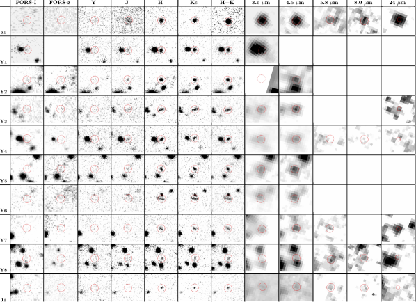
Figure 11: Thumbnail images of the bright $z$, $Y$ and $J$-dropouts found in A2667, covering a $9^{\prime\prime}\times 7.3^{\prime\prime}$ area on the original images from $I$ band to 8.0$\mu$m, and $18^{\prime\prime}\times 14.6^{\prime\prime}$ for MIPS 24$\mu$m. The position of each candidate is displayed by a circle of 2″diameter aperture. Images are displayed in linear scale ranging between -5 and 20 $\sigma$ around the sky background.

Only one candidate, J1, fulfills the selection criteria (b) based on $JHKs$, and is also consistent with the z$\sim$9 $J-$drop selection criteria by Bouwens et al. (2010) (see Fig. 3). This object was formally detected in the $I$ band at $\,\stackrel{{\scriptstyle<}}{{\scriptstyle\sim}}\,$2$\sigma$ level (double-image mode), as indicated in Table 3, although no convincing counterpart is seen in this image (see also Fig. 11). This source has a counterpart detected on the HST F850LP/ACS image, as discussed in Sect. 4.1 below.

It is worth noting that all $Y$-dropout candidates excepted z1 are too faint to be selected by the original Capak et al. criteria (i.e. intrinsic lensing-corrected $J$$\,\stackrel{{\scriptstyle>}}{{\scriptstyle\sim}}\,$24, see below). When the same color selection (c) is applied to fainter $J$-band magnitudes, up to $J<$ 25.7 (our own 5$\sigma$ detection level), 22 objects are selected after manual inspection. Among them, all our Y candidates except Y4 are found. Indeed, Y4 was formally detected in the reference $z$ band at $\,\stackrel{{\scriptstyle<}}{{\scriptstyle\sim}}\,$2$\sigma$ level (as indicated in Table 3, double-image mode), although there is no clear counterpart seen on this image and it is also not detected in the $z_{2}$ field. This sample of fainter $z$-dropout candidates will be discussed elsewhere in a forecoming paper.

Hereafter we concentrate on the bright $z$-dropout z1 and the nine $Y$ and $J$-dropout candidates. We have checked for all these objects that their spectral energy distribution (hereafter SED) remains the same when using SExtractor aperture and MAG_AUTO magnitudes. MAG_AUTO magnitudes were preferred for the subsequent analysis because they are closer to total magnitudes.

4 Results

4.1 Observed properties of the high-$z$ candidates

The identification, position and morphology of the ten bright $Y$ and $J-$dropouts selected in this field is given in Table 2. Table 3 summarizes their photometric properties, and Fig. 11 displays the corresponding postage stamps. Except for J1, all candidates are detected in the $J$, $H$ and $Ks$ bands. The observed $H$ and $Ks$ band magnitudes of our objects range typically from $\sim$ 23 to 25, i.e. in a regime where our sample is close to 100% complete. For the high-$z$ candidates in the common area between $z_{1}$ and $z_{2}$ fields of view (namely z1, Y3, Y4, Y5, Y6, Y8 and J1), we have also cheched the independent non-detection on the two original images.

The SExtractor stellarity index and the FWHM along the major axis, both measured on the $H+Ks$ detection image, were used to quantify the morphology of our candidates. This information was only used to assess the possible contamination by cool stars, in addition to colors. The reliability of the SExtractor stellarity index for galaxies diminishes towards the faintest magnitudes. We have checked that a reliable index can be obtained up to $HK\sim$24.5 for our combined image, becoming hazardous for fainter sources and highly unreliable at $HK\geq$25.0, where the S/N significantly drops below $\sim$10. From Table 2 it appears that all our sources seem to be inconsistent with stars, except Y8 and J1 which are too faint for a robust morphological classification based on the detection image. As shown in Fig. 2 to  4, all candidates but Y8 display colors which are clearly incompatible with cool stars.

J1 is the only candidate located on the central area covered by the HST F850LP/ACS image. A faint and compact object is indeed detected on this image, with FWHM$\sim$0.1″(Sextractor stellarity parameter is 0.7), and $z_{850}=$27.39$\pm$0.18 (MAG_AUTO on the original HST image). This magnitude is fully consistent with the non-detection on the ground-based $z$-band images (AB$\sim$27.2 at 1$\sigma$ level), and confirms the important break between optical and near-IR bands for this object, which is the faintest one in our sample.

Good quality magnitudes were extracted for six and seven sources on the IRAC 3.6$\mu$m and 4.5$\mu$m images respectively. For the remainder, only partial data is available (Y1, Y2), or the photometry is strongly contaminated by nearby sources (see Fig. 11). The only candidates clearly detected and reported in Table 3 for the shallow 5.8$\mu$m and 8.0$\mu$m images are z1, Y8 and J1, even though magnitudes are dubious for Y8 and J1 due to a noisy environment. Two objects, z1 and Y7, are clearly detected on the MIPS 24$\mu$m image.

4.2 Magnification of the drop-out sources

The lensing model for A2667 was originally obtained by Covone et al. (2006). We use this model to compute the magnification maps at different source redshifts with the public lensing software Lenstool, including the new MCMC optimization method (Jullo et al. 2007) providing bayesian estimates on model parameters.

The mass model was used to derive the magnification factor for each object and associated error bars, both for the high and low-z solutions (i.e. typical redshifts of $z\sim 7.5$-9.0 and $z\sim 1.7$-2.0 respectively, see Sect. 4.3). These values are given in Table 2. The magnification factors of our objects typically range between 1.1 and 1.4, e.g. $\sim$0.4 mags being largest for Y4 and J1. None of these candidates is expected to be a multiple image.

Given the location of our candidates with respect to the critical lines, either in the high or in the low-z solutions, the uncertainty in the magnification associated to the uncertainty on the redshift is smaller than 10% in all cases. Also the magnification factor at a given position on the image plane varies slowly with redshift for sources located more than $\sim 10^{\prime\prime}$ apart from the critical lines, and this is indeed the case for all our candidates. Error bars in magnification are also given in Table 2, including both uncertainties on source redshift and systematic errors due to the choice of the parametrization in lensing modelling (see e.g. Maizy et al. 2010). We also used this lensing model to compute the effective surveyed area and volume around $z\gtrsim$7.5 when comparing with blank field surveys. All surface and volume number-densities given in this paper have been corrected for magnification by the lensing cluster.

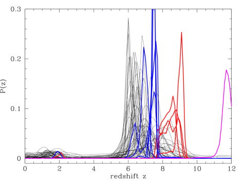
Figure 5: Redshift probability distributions, $P(z)$ for our objects computed using standard templates (BC solar metallicity, no emission lines). Objects Y1, Y3, Y6, Y8, and z1 are shown in blue, Y2, Y4, Y5, and Y7 in red, and J1 in magenta. Black lines show $P(z)$ of other $z\sim$ 6–8 galaxies from HST surveys using NICMOS and WFC3 from the analysis of Schaerer & de Barros (2010), namely Gonzalez et al. (2010) and McLure et al. (2010) sample)

4.3 SED fitting results: photometric redshifts

Photometric redshifts and associated probability distributions were derived for each one of our candidates from the available broad-band photometry, except for the 24$\mu$m MIPS photometry, which is only available for a few candidates (see discussion below in Sect. 4.6). A modified version of the public photometric redshift software $Hyperz$ (Bolzonella et al. 2000) was used, adapted to include nebular emission (see Schaerer & de Barros 2009, 2010, hereafter SB2010). The following spectral templates were used for our SED fits: empirical templates (starbursts from Kinney et al. 1996; galaxies from Coleman et al. 1980; GRASIL templates from Silva et al. 1998, and the UV-to-radio templates of galaxies and AGN from Polletta et al. 2007), and Bruzual & Charlot (2003; hereafter BC) evolutionary sythesis models to which nebular emission (lines and continua) is added optionally.

The free parameters for the SED fits are the metallicity $Z$ (ranging from $\sim$1/50 $Z_{\odot}$ to $Z_{\odot}$), the star-formation history, the age since the onset of star-formation, extinction and redshift. For empirical templates redshift is in principle the only free parameter. However, in some cases we also allow for additional, variable extinction for empirical templates. Extintion is varied from $A_{V}=0$ to 4 in steps of 0.2 mag, using the Calzetti et al. (2000) extinction law. The Lyman forest blanketing is included following the prescription of Madau (1995).

The non-detection in the $I$, $z$, $Y$ and $J$ bands was used as a constraint when computing photometric redshifts. Unless otherwise indicated, the rule applied corresponds to the usual case “1” of $Hyperz$, i.e. the flux in these filters is set to zero, with an error bar corresponding to the flux at 1$\sigma$ level, using both the global value and the local sensitivity computed near each source (see below). We have also computed photometric redshifts by forcing the fluxes in these filters to be below 2$\sigma$ and 3$\sigma$ levels using case “2” of $Hyperz$ for non-detections. As explained below, the results obtained are rather insensitive to the non-detection rule and sensitivity applied (local or global). A minimum error bar of 0.1 magnitudes was assumed for IRAC photometry to account for uncertainties in absolute flux calibrations when combining with the other filters.

The resulting redshift probability distributions $P(z)$ for all our objects, obtained with standard Bruzual & Charlot, solar metallicity templates, is shown in Fig. 5. $P(z)$ displayed in this Figure were obtained using the $Hyperz$ approach, i.e. $P(z)\propto exp(-\chi^{2}(z))$, which is very similar to the results derived from Monte Carlo simulations. As shown by this Figure, most objects have a relatively well defined redshift probability distribution $P(z)$ peaking at high redshift. Five objects (Y1, Y3, Y6, Y8, and z1) show best-fit redshifts $z_{\rm phot}$ $\sim$ 7–8, four objects (Y2, Y4, Y5, and Y7), a higher redshift $z_{\rm phot}$ $\sim$ 7.5–9.5, and for the $J-$drop J1 $z_{\rm phot}$ $>$9.5 is favoured. These redshift ranges and their relative grouping are consistent with expectations from their colors (cf. Fig. 2). For most objects a less significant solution is found at low-$z$, in general within $z\sim$ 1.7 and 2.8. However, even though the high-$z$ solution produces a better fit, several of these sources seem too bright (M${}_{1500}<-23.0$) to be at $z\geq 7.5$, suggesting some contamination by low-$z$ interlopers. This issue will be discussed below.

Fig. 5 also displays for comparison the $P(z)$ derived by SB2010 for a recent sample of $z\sim$ 6–8 galaxies including objects from HST surveys using NICMOS and the recent WFC3 camera. The corresponding $P(z)$ of our candidates compare to and overlap these samples, and our selection function has clearly favoured the $z>$7 domain.

Using standard spectral templates (neglecting the effects of nebular emission) we obtain the best-fit photometric redshifts and physical parameters given in Table 4. We have also examined how the inclusion of nebular lines and continuous emission may alter the photometric redshift. In Fig. 6 and Table 4 we show the best-fit SEDs for all our objects in two different cases: without any redshift prior, and with the restriction of $z<4$. In all cases the best-fit is found at high $z$, irrespective of the inclusion or not of nebular emission. Low redshift solutions (typically at $z\sim$ 1.7–2.1 and $z\sim$ 2.5–2.8 for J1), show fits of lower quality, especially close to the spectral break and between $Y$, $J$, and $H$, as could be expected from the behaviour of spectral templates in these colours. Furthermore, these best-fit, low redshift solutions show generally excess in the optical bands ($I$, $z$) indicating that most of these objects should be detected at a 3–5 $\sigma$ level in at least one of these bands. Note, that in some cases the inclusion of nebular emission allows for somewhat ”unexpected” solutions with strong emission lines plus a high attenuation (see e.g. the fits for z1, Y8, and J1), although the resulting low-$z$ fits remain with a higher $\chi^{2}$.

We have investigated the influence of non-detection rules and limiting fluxes on photometric redshifts results. When applying a local non-detection limit instead of the global one, there is no difference in the high-$z$ solutions (similar $\chi^{2}$ and $\Delta$z$<$0.1). Low redshift fits display the same lower quality as compared to high-$z$, with similar $\chi^{2}$ and, in general, $\Delta$z$\sim$0.1, although there are larger differences for Y2 ($\Delta$z$\sim$1), Y4 ($\Delta$z$\sim$0.4) and Y5 ($\Delta$z$\sim$0.2). As shown in Table 4, the same differences in $\Delta$z are observed when comparing the photometric redshifts achieved with local non-detections and the standard $Hyperz$ models, with those found with global non-detections and the complete library (including nebular emission). In other words, the dispersion in photometric redshifts between local and global non-detection limits is similar to the dispersion due to model uncertainties. And, in all cases, the high-$z$ solution is privileged.

We have also computed photometric redshifts by replacing the non-detection rule “1” of $Hyperz$ by rule “2” in all filters where the candidates are formally not-detected, where the flux and the error bars are set to $F_{\rm lim}/2$, for two different cases, $F_{\rm lim}$=2$\sigma$ and 3$\sigma$ detection levels. Best-fit redshifts remain precisely the same for most of our candidates at 2$\sigma$ level, the only exception being Y8 (degenerate solution with best fit at z$=$1.7). When the fluxes are allowed to reach a 3$\sigma$ level, three other objects become degenerate, with a best-fit at low-$z$, namely Y6, Y7 and J1. Table 4 summarizes the integrated probability distribution at z$>$6 for all candidates when using different assumptions for non-detections.

As mentioned above, there is some overlap between the $z$ and $Y$ bands, but the $Y-$band allows us improving photometric redshifts. Indeed, when SED fitting results are derived without $Y-$band data, we still obtain a best-fit at high-$z$ for all objects. The $P(z)$ distribution for all objects detected in $Y$ (blue lines in Fig. 5) becomes broader (from $z_{\rm phot}$  well peaked at 7–8 to $z_{\rm phot}$ $\sim$ 6.5–9). For all other objects the changes in $P(z)$ are minor. When both $Y$ and $J-$band data are removed, this strongly degrades the photometric redshift $P(z)$ distribution and $z_{\rm phot}$  becomes basically undefined for all objects.

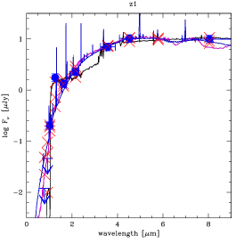
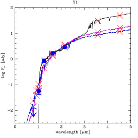
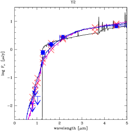
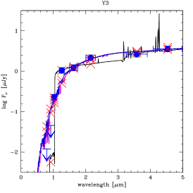
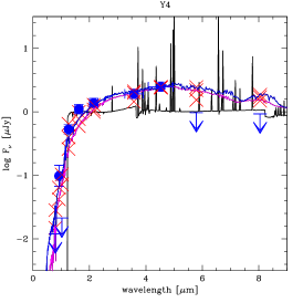
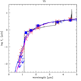
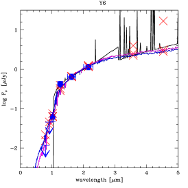
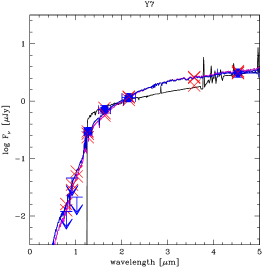
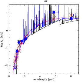
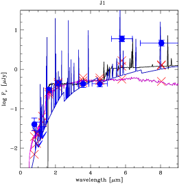
Figure 6: Best-fit SED solutions for high-$z$ (black lines) et low-$z$ (blue and magenta lines) for all the bright $z$, $Y$ and $J-$dropouts found in A2667. Error bars and upper limits correspond to 1$\sigma$ values, as reported in Table 3. Red crosses indicate the synthetic flux in the filters. High-$z$ (black) spectra include nebular emission. Low-$z$ solutions are displayed for the complete library (including nebular emission) in blue, and for the standard templates in magenta. Note the extended wavelength scale for objects with available 5.8 and 8.0 $\mu$m photometry.

Table 4: Properties of bright $z$, $Y$ and $J-$dropouts in A2667.

Source	$z_{phot}$	$\chi^{2}$	$z_{min}-z_{max}$	$A_{V}$	M1500	L1500	SFR	$z_{phot}$	$\chi^{2}$	$A_{V}$	MB	P(z$>$6)
	high-$z$					$\times$1041		low-$z$				(1)	(2)	(3)	(4)
						erg/s/cm2	M⊙/yr
z1 (a)	7.6	75.08	7.5-7.7	0.3	-23.44	13.7	144	1.78	228.27	2.4	-20.06	1.0	1.0	1.0	1.0	(low)
(b)	7.6							1.94
Y1 (a)	7.7	0.02	7.2-7.8	2.4	-23.12	10.2	108	1.72	39.62	0.3	-19.82	1.0	0.0	1.0	1.0	low
(b)	7.4							1.65
Y2 (a)	8.7	0.89	7.7-9.3	2.4	-23.53	14.9	157	2.72	38.01	0.0	-21.78	1.0	0.0	1.0	0.99	low
(b)	9.1							2.11
Y3 (a)	7.5	28.68	7.3-7.6	1.2	-22.97	8.9	94	1.88	72.94	0.6	-20.32	1.0	0.97	1.0	0.79	high
(b)	7.5							1.95
Y4 (a)	9.1	6.98	8.7-9.4	1.2	-23.14	10.4	110	2.58	73.71	0.0	-21.13	1.0	1.0	1.0	0.99	high
(b)	9.2							2.11
Y5 (a)	8.6	10.82	7.7-8.8	2.1	-22.97	8.9	94	1.70	40.95	0.0	-19.32	1.0	0.63	1.0	0.98	?
(b)	8.3							1.94
Y6 (a)	7.5	0.14	6.6-7.7	1.2	-22.15	4.2	44	1.94	3.64	1.50	-19.74	0.94	0.0	0.55	0.46	low
(b)	7.5							1.87
Y7 (a)	9.1	0.05	8.0-9.4	1.8	-22.90	8.3	87	1.72	10.5	0.3	-18.87	0.99	0.0	0.93	0.41	low
(b)	9.2							2.11
Y8 (a)	7.4	0.02	5.9-7.7	0.3	-21.29	1.9	20	1.66	0.77	0.6	-18.33	0.82	0.05	0.37	0.26	low
(b)	7.4							1.70
J1 (a)	11.9	4.93	9.6-12.0	0.0	-22.66	6.7	71	2.80	12.48	0.0	-20.19	1.0	0.94	0.85	0.20	(low)
(b)(c)	11.8							2.50

4.4 Quality grades

Table 2 includes two different quality grades for each source representing its likelihood to be a genuine high-$z$ candidate. The first one is based on the quality of the photometric information gathered for the source in terms of surrounding environment, completeness of the SED and intrinsic UV luminosity if at high-$z$. The second grade is based on the robustness of the optical non-detection criteria, following Bouwens et al. (2010).

The first grade $Q$ includes three independent criteria introduced as follows:

• The first one ($Q1$) is the quality of the surrounding environment, representing the possible contamination by neighbouring or underlying sources. Although all candidates are isolated on the good-seeing detection image $H+Ks$, the presence of another source within a distance of 2″is given the lowest grade (=1), whereas isolated candidates without neighbours closer than $\geq$3″have the highest grade (=3).

• The second one ($Q2$) is the quality of the photometric SED. Objects with robusts constraints available beyond the $Ks$ band, including 5.8 and 8.0 $\mu$m bands, are given the hightest grade (=3). The lowest grade (=1) is given to sources lacking one or several bands at $\lambda\leq$4.5$\mu$m, either because of field coverage or because of confusion problems.

• The third one ($Q3$) is the UV luminosity of the candidate at the best-fit photometric redshift, after correction for lensing effects. The hightest (=3) and the lowest (=1) grades are given respectively to sources fainter than 3$L^{*}$ and brighter than $\sim$10$L^{*}$, where $L^{*}$ stands for the Reddy & Steidel (2009) value assuming no evolution.

As a result of these criteria, the most likely sources are given the highest cumulated value of $Q=Q1+Q2+Q3$, allowing us to define a final grade which represents the quality of a given candidate, ranging between 3 and 9 (for an ideal candidate). As seen in Table 2, four candidates achieve the highest rates, between $Q=$7 (z1) and $Q=$8 (Y3, Y7 and J1). In all these cases, the high intrinsic luminosity is responsible for a lower value of Q3 with respect to the ideal case. These sources are considered as highest quality or category I. Three candidates achieve a fair value of $Q=$6 (Y4, Y5 and Y8) and are therefore considered as reasonably good (category II) candidates. The lowest grade (category III) is achieved for sources with close neighbours potentially affecting the quality of the global SED (Y1, Y2 and Y6).

The second grade is given by the optical $\chi^{2}_{opt}$ computed on the optical bands as follows (see also Bouwens et al. 2010):

$$\chi^{2}_{opt}=\sum_{i}SGN(f_{i})(\frac{f_{i}}{\sigma_{i}})^{2}$$ (1)

where $f_{i}$ is the flux in the band $i$, $\sigma_{i}$ is the corresponding uncertainty, and $SGN(f_{i})$ is equal to 1 if $f_{i}>$0 and equal to -1 if $f_{i}<$0. We have used $IRAF$ package $qphot.apphot$ to measure fluxes in a 1.3” diameter aperture, together with the corresponding noise in the neighbouring sky region. $\chi^{2}_{opt}$ values reported in Table 2 are based on $I$ and $z$-band images. In the case of J1, the $Y$-band was also included in the $\chi^{2}_{opt}$ calculation. Straightforward simulations were conducted in order to determine the $\chi^{2}_{opt}$ distribution expected for truly non-detected sources as well as for sources at different S/N values, in particular for those close to the 2$\sigma$ non-detection criteria in $I$ and $z$. All genuine non-detected sources exhibit $\chi^{2}_{opt}<$ 2, with 90% at $\chi^{2}_{opt}<$ 1 level, whereas only 3% of sources with S/N$\sim$2$\sigma$ in $I$ and $z$ are found with $\chi^{2}_{opt}<$ 2 (1% with $\chi^{2}_{opt}<$ 1). As seen in Table 2, all our candidates exhibit $\chi^{2}_{opt}$ $\,\stackrel{{\scriptstyle<}}{{\scriptstyle\sim}}\,$1, the highest values corresponding to Y1 and Y2 (already ranked among the category III above).

These two quality grades above provide a useful priority for spectroscopic follow up, although they do not take into account all the details regarding SED-fit constraints, as discussed below, which are somehow model-dependent. In particular the 24$\mu$m emission, which is difficult to reconcile with a high-$z$ identification for z1 and J1 despite a high grade. Also the detection of J1 on the HST $z_{850}-$band favours a low-$z$ solution for this source, which is considered hereafter as a possible interloper.

4.5 Photometric redshifts with a luminosity prior

Given the luminosities derived for these candidates in the high-$z$ hypothesis, leading to rather extreme masses and star-formation rates, it seems likely that, despite a best-fit at high-$z$, a large fraction of them actually corresponds to low-$z$ interlopers. In order to better quantify this contamination, we have introduced a luminosity prior when computing photometric redshifts.

A prior probability distribution was introduced as a function of redshift and magnitude, following Benitez (2000). In this case, the prior probability is the redshift distribution for galaxies of a given apparent magnitude $m$. Given the wide redshift domain covered by the $P(z)$, and the fact that we are likely dealing with either genuine high-$z$ or $z\sim$1.5-2.5 star-forming galaxies, we computed the prior probability based on the luminosity function for star-forming galaxies in the $B$-band (Ilbert et al. 2005). This band is indeed directly “seen” by the SED of galaxies in our sample for all redshifts between $z\sim$0.8 and 9. A smooth probability distribution prior was computed for each object as a function of redshift, with the absolute magnitude M_B derived from the apparent magnitude $m$ which is closer to the rest-frame $B$-band. The final probability distribution is given by the previous $Hyperz$ $P(z)$ multiplied by the prior.

Fig. 7 displays the resulting probability distributions for all candidates, arbitrarily normalized to 100 between $z=$0 and 12. As seen in this figure, four candidates still exhibit a dominant high-$z$ solution, namely z1, Y3, Y4, and J1, whereas one candidate is degenerate between low and high-$z$ (Y5). The best high-$z$ candidates also exhibit the better quality grades, as seen in previous section. We use these results to propose a final tentative classification between likely low-$z$ interlopers and high-$z$ candidates in Table 2. Despite a high grade, z1 and J1 are ranked among the likely low-$z$ contaminants based on the detections in the 24$\mu$m and $z_{850}$ bands respectively.

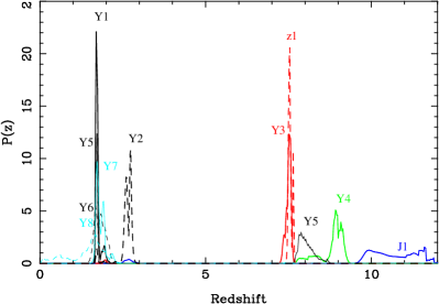
Figure 7: Redshift probability distributions for the sample of high-$z$ candidates, arbitrarily normalized to 100 between $z=$0 and 12, resulting from $Hyperz$ $P(z)$ multiplied by a smooth luminosity prior.

4.6 Physical properties from SED fits

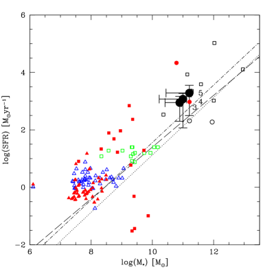
Figure 8: Mass–SFR relation of the $z$, $Y$, and $J$-dropout galaxies resulting from $10^{3}$ Monte Carlo simulations compared to the properties of $z\sim$ 6–8 galaxies from recent surveys analysed by Schaerer & de Barros (2010). The most likely high-$z$ candidates based on photometric redshifts with a luminosity prior, namely Y3, Y4 and Y5, are identified and displayed by large black dots. The positions derived for the other optical-dropouts in this study, if at high-$z$, are indicated by black open squares for comparison. Open symbols (squares, triangles) show the “standard” SFR(UV) value (not corrected for extinction) versus mass derived from the SB2010 reference model for objects from their bright, intermediate, and faint samples respectively. Red filled symbols show the best-fit model SFR and $M_{\star}$ values when assuming $\tau\geq 10$ Myr (model 1 in SB2010). Circles correspond to the 2 objects from Capak et al. 2011). The dotted (dash-dotted) lines show the locus for ${\it SFR}={\rm const.}$ from $z=\infty$ (10) to 7 corresponding to ${\it SSFR}=1.3$ (3.6) Gyr-1. The dashed line shows the relation found by Daddi et al. (2007) for $z\sim 2$ star-forming galaxies. The large spread in SFR is in particular due to the fact that a wide variety of exponentially decreasing star-formation histories are allowed. Note that if at high redshift the properties of our galaxies follow the trends observed for less massive/bright objects a high redshift.

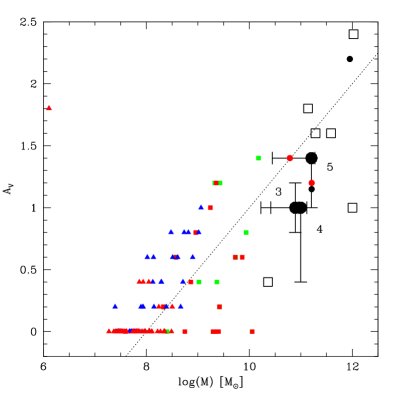
Figure 9: Mass–AV relation for the same objects as shown in Fig. 8 (same symbols).

From our SED fits using the Bruzual & Charlot templates we can also derive the physical properties of the galaxies, such as the age of the stellar population, the stellar mass, star-formation rate, and attenuation. The resulting masses, SFR, and attenuation $A_{V}$ (derived assuming the Calzetti law) and the uncertainties, derived from 1000 Monte Carlo simulations of each object, are shown in Figs. 8 and 9. For comparison we also show the properties of $z\sim$ 6–8 galaxies analysed recently by SB2010 using the same SED fitting tool.

As can be seen, the masses derived for the most likely high-$z$ candidates based on photometric redshifts with a luminosity prior, namely Y3, Y4 and Y5, are among the highest masses found by SB2010, typically of the order of $M_{\star}\sim 2\times 10^{10}$ to $2\times 10^{11}$ ${\rm M_{\odot}}$. Including relatively large corrections for attenuation ($A_{V}\sim$ 0.4–1.4), their SFR range from $\sim$ 100 to $\sim 10^{3}$ ${\rm M_{\odot}yr^{-1}}$. For comparison, the SFR derived from the rest-frame UV luminosity L₁₅₀₀ using the Kennicutt (1998) calibration is typically $\sim$ 100 ${\rm M_{\odot}yr^{-1}}$for these sources (see Table 4).

When including the full sample of optical-dropout candidates, the masses and SFRs achieved are much larger, reaching $M_{\star}\sim 10^{12}$ ${\rm M_{\odot}}$ in most cases, and even $M_{\star}>10^{12}$ ${\rm M_{\odot}}$ for the brightest $Y$-drop candidate, Y1, if at high-$z$. However, for the most extreme objects the uncertainties on $A_{V}$ and SFR are very large. For objects with well defined errors, the SFR may reach up to 2000-3000 ${\rm M_{\odot}yr^{-1}}$. Interestingly enough these values are not in disagreement with the trends found by SB2010 for the fainter $z>6$ galaxies from recent HST surveys, if extrapolated to higher masses. These properties are also similar to those of the two $z\sim 7$ galaxy candidates found by Capak et al. (2011) in the COSMOS wide field survey. However, whether these relatively bright objects are truely high redshift galaxies, and hence objects with such extreme properties, remains of course questionable (see below).

Two of our optical dropout galaxies (z1 and Y7) are detected by MIPS at 24 $\mu$m with fluxes 3.4 and 1.1 $\times 10^{-4}$ Jy respectively, and we have non-detection constraints for three additional sources included in the MIPS image (Y3, Y4 and J1, with 1$\sigma$ fluxes below 38.7 $\mu$Jy), whereas Y8 is highly contaminated by neighbouring galaxies (see Fig. 11). Recently, two objects of this sample have also been detected with Herschel and LABOCA between 160 and 870 $\mu$m (Boone et al., in preparation). This data identifies z1 and Y5 as mid-$z$ interlopers.

For $z\sim$ 1–2 galaxies the MIPS band probes a region in the mid-IR corresponding or close to redshifted PAH emission. If at high redshift ($z\sim$ 7–9), the 24 $\mu$m band samples the region between 2–3 $\mu$m. To illustrate the overall SED of our MIPS-detected (or constrained) objects we show their photometry together with several SED fits in Fig. 10. In addition to our standard spectral templates with/without nebular emission we also show best-fits using (semi)empirical templates of nearby galaxies including in particular very dusty galaxies, LIRG, and ULIRG. In practice we have used the templates from the GRASIL models of Silva et al. (1998), the SWIRE starburst-AGN templates of Polletta et al. (2008), and LIRG–ULIRG templates of Rieke et al. (2009); redshift and additional extinction are kept as free fit parameters. For all of these models we here show the best-fits under the constraint that $z<4$ and without any constraint. We note that the best-fit photometric redshifts at low-$z$ can differ quite significantly depending on the set of spectral templates used and between the objects. For example, we find $z_{\rm phot}$ $\sim$ 0.1, 1.5, and 2.7 for Y3; 1.6–1.7 for Y7, 0.02, 1.6, and 1.6 for Y8, and 0.1–0.5 for J1. Furthermore the 24 $\mu$m flux expected from these fits can vary by more than an order of magnitude. Interestingly fits at high-$z$ show fluxes at 24 $\mu$m which are comparable to those expected from some of low-$z$ best-fits, thus providing weak additional constraints on the redshift.

Several objects in this sample deserve additional specific comments.

• z1: This is the brightest source in our sample. It is an extended isolated object, clearly non-stellar. It is detected in all filter bands between $Y$ and 24$\mu$m  except at 5.8$\mu$m where no data is available. Although the best-fit is obtained at high-$z$, even with a luminosity prior, the 24 $\mu$m flux seems incompatible with the high-$z$ solution (see Fig. 10). It appears even too bright in this band when compared to the best-fit templates at low-$z$. However, the observed flux in the $J-$band, and the fact that, if at low-$z$, it should be also detected in the $I$ and $z$ bands at $\geq$ 3 $\sigma$ level (given the depth of our survey), remain difficult to explain.

• Y3: Although the 24 $\mu$m non-detection of this object helps to exclude at least one of the GRASIL templates at low-$z$, it is still consistent with other templates at low and high-$z$. Probably the main failure of the low-$z$ templates is again the mismatch in $J$ and in the optical bands.

• Y4: As for Y3, the upper limit detection at 24 $\mu$m provides weak additional constraints on the redshift. The non-detection at 5.8 and 8$\mu$m are interesting because both solutions at low and high-$z$ seem to predict a detection at $\sim$2-3$\sigma$ level. The object is formally detected at the $\,\stackrel{{\scriptstyle<}}{{\scriptstyle\sim}}\,$$2\sigma$ level in the $z_{1}$ band, but it is not detected in the $z_{2}$ image.

• Y7: For this object, the expected 24 $\mu$m fluxes for the best-fit at high and low redshifts are very similar. In particular, the flux of the $z\sim 9$ fit is even quite similar to the brightest flux predicted from dusty galaxy templates at $z\sim 1.6$. Therefore, this object cannot be excluded as a genuine high-$z$ based on its MIPS photometry without introducing a luminosity prior. Besides, the observed 24$\mu$m flux seems too high irrespective of the template redshift for a relatively isolated source (see Fig. 11).

• Y8: The 5.8 and 8$\mu$m photometry for this object could be seriously contaminated by bright neighboring sources (see Fig. 11), although this seems to be the only emission at this precise location. The 24 $\mu$m flux shown in Fig. 10 corresponds to the lower limit, and it is compatible with both the low and the high-$z$ solutions.

• J1: This is the faintest candidate in our sample, and the only one which is located on the central area covered by the HST. The best-fit solution is found at high-$z$ even when including the $z_{850}-$band flux and a luminosity prior, as seen in Table 4. However, the detection on the $z_{850}-$band makes the high-$z$ solution unlikely. The upper limit detection at 24 $\mu$m provides weak additional constraints on the redshift. The detection on the HST image is fully consistent with the large break identified on ground-based images. The apparent strong “double-break” between the optical/near-IR and between 4.5/5.8 $\mu$m seems quite unusual. High-$z$ solutions have difficulty reproducing the latter break (see Fig. 6), while low-$z$ solutions predict a flux excess in the optical domain. The break at 4.5–5.8 $\mu$m could be explained by PAH features boosting the 5.8 and 8 $\mu$m fluxes, as shown in Fig. 6. This is one of the candidates for which a spectroscopic follow up is needed to conclude.

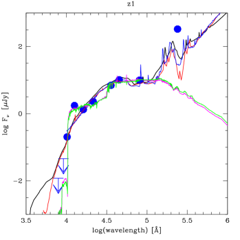
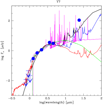
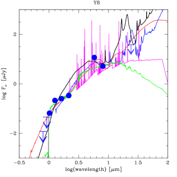
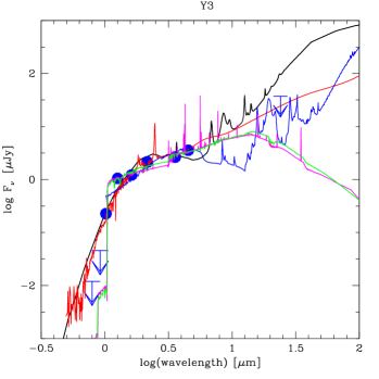
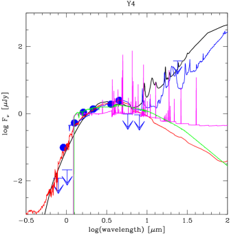
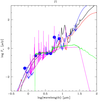
Figure 10: Best-fit SEDs for candidates with available constraints at 24 $\mu$m : z1 and Y7 (sources clearly detected, top row), Y8 (source highly contaminated, middle left panel), and Y3, Y4 and J1 (non-detection, 1$\sigma$ flux $<$ 38.7 $\mu$Jy). Different spectral templates are displayed. Green (pink) lines show the best-fit solutions at $z>7$ using our standard templates based on Bruzual & Charlot models without (with) nebular lines. Black and red lines show the best-fits at low redshift ($z<4$) using the templates from the GRASIL models (Silva et al. 1998) and the SWIRE starburst-AGN templates of Polletta et al. (2008) respectively. Blue lines show best-fits using the empirical LIRG–ULIRG templates of Rieke et al. (2009).

4.7 Contamination level based on stacked images

Based on previous discussions, a large fraction of optical-dropout galaxies in this sample could be low-$z$ contaminants, reaching as high as $\sim$70% based on luminosity priors. In order to better quantify this estimate, we have generated stacked images in the $I$ and $z$ bands, where genuine high-$z$ galaxies are not expected to be detected. On the contrary, the S/N ratio achieved on the stacked image should allow us to estimate the contamination level.

For each candidate, a 10″$\times$ 10″region has been selected in the $I$ and $z$-band images around the centroid position on the detection image $H+Ks$. An additive zero level correction has been applied to each single image to properly remove the local average sky background. $I$ and $z$-band images have been averaged using IRAF routines and different pixel rejection schemes in order to improve the suppression of neighboring sources on the final combined images. Due to the presence of a closeby galaxy, we do not include the Y1 field in the final stacks. We have checked that the sky backgound noise on the final combined images actually improves as expected as a function of the total number of images stacked, i.e. reaching a reduction by a factor close to 3 on the final stacks with respect to the original images.

We used IRAF routines to measure fluxes and magnitudes in a 1.3” diameter aperture, together with the corresponding error bars on the different stacks. The best S/N ratio is achieved in the $I$-band, where we measure up to $I=$28.0$\pm$0.3 for the combined source, i.e. a S/N$\sim$3. The detection in the $z$-band is less significant, reaching $z=$27.7$\pm$0.5 (S/N$\sim$2) on the best-detected final stack. These results confirm that there is indeed some contamination by low-$z$ interlopers in our sample. The detection level in the $I$-band is roughly consistent with $\sim$70% of the sample being detected at $\sim$1$\sigma$ level, although 3-4 objects detected between 1 and 2 $\sigma$ would be enough to account for the signal in this band. The flux measured in the $z$-band seems to favour either a signal below 1$\sigma$ for a large majority of our candidates, or a higher signal coming from a small fraction of contaminants (between $\sim$20% with S/N$\la$2, or $\sim$30% with a mean S/N$\sim$1.5).

5 Discussion

As the selection diagrams (Figs. 2 and 3) show, most of our bright candidates have near-IR colors distinguishing them clearly from normal galaxies at low redshift and late type stars. Also SED-fitting results clearly favor a high-$z$ solution for all these candidates, irrespective of their intrinsic luminosities. However, as seen in Table 4, high-$z$ solutions yield magnification-corrected luminosities which typically range between 3 times (Y8) and 40 times (z1, Y2) L${}_{1500}^{*}$ at these redshifts, according to the evolving LF by Bouwens et al. (2008), suggesting a potential contamination by low-$z$ interlopers. In this section we discuss the observed versus expected number counts of high-$z$ galaxies, and the possible sources of contamination in our survey. We also compare our results and the properties of this sample with those obtained by previous authors using similar techniques.

5.1 Observed versus expected number density of high-$z$ sources

We first compute the expected number counts of bright high-$z$ sources in this lensing field, as a function of redshift and for the range of magnitudes of our candidates (i.e. AB$\sim$23 to 25.5), and we compare these numbers with current observations. This calculation was done following the same procedure as in Maizy et al. (2010). All the noisy regions in the field, in particular around bright galaxies in the cluster core, have been masked. The presence of a strong lensing cluster in this field introduces two opposite effects on the number counts as compared to blank fields. Gravitational magnification increases the number of faint sources by improving the detection towards the faint end of the LF, whereas the dilution effect reduces the effective volume by the same factor. As discussed in Maizy et al. (2010), the difference between lensing and blank field results depends strongly on the shape of the LF. We expect lensing clusters to be more efficient than blank fields in relatively shallow surveys.

Number counts of sources brighter than a limiting magnitude were computed by a pixel-to-pixel integration of the magnified source plane as a function of redshift (see eq. 6 in Maizy et al. 2010), for redshift bins $\Delta z=1$, using the evolving LF by Bouwens et al. (2008), i.e. with the Schechter parameters directly derived from eq. 3 in their paper. For comparison purposes, we also derive the expected counts with the Beckwith et al. (2006) LF for $z\sim 6$ galaxies, assuming no evolution. This LF displays the same Schechter parameters as for Steidel et al. (2003) and Reddy & Steidel (2009), but the normalization factor is 3 times smaller than for Steidel et al. (2003). Table 5 summarizes these results for two different limiting magnitudes, AB$<$25.5, where all the current candidates are found, and AB$<$26.0, which corresponds to our $\sim$5$\sigma$ detection level (in the filter spanning the UV region around 1500Å ). Error bars include Poisson uncertainty and field-to-field variance, following Trenti & Stiavelli (2008). Given the small number counts expected, these fluctuations dominate the error budget (see also the discussion in Maizy et al. 2010). We also computed number counts using the latest Schechter parameters presented by Bouwens et al. (2010) for galaxies at $z\sim$7 in the $z=[7.0,8.0]$ interval, and for galaxies at $z\sim$8 in the $z=[8.0,9.0]$ interval (identified by $*$ in Table 5). The changes with respect to the 2008 version are relatively minor in this case given the luminosity domain, which is largely dominated by statistical uncertainties.

Table 5: Number counts of sources with AB$<$25.5 and AB$<$26.0 expected in the field of A2667, with and without the presence of a lensing cluster, for different redshift bins and for two different LFs: Bouwens et al. 2008 (1) and Beckwith et al. 2006 (2) (see text). Error bars in number counts, including Poisson uncertainty and field-to-field variance, are given in brackets.

	LF(1)		LF(2)
Redshift	Blank	A2667	Blank	A2667
AB$<$25.5
$[6.0,7.0]$	0.5 (1)	1.5 (2)	2.9 (3)	4.2 (3)
$[7.0,8.0]$	$<$0.1 (1)	0.3 (1)	1.5 (2)	2.3 (2)
(*)	0.1 (1)	0.5 (1)
$[8.0,9.0]$	$<$0.1 (1)	0.1 (1)	0.8 (1)	1.4 (2)
(*)	$<$0.1 (1)	0.2 (1)
$[9.0,11.0]$	$<$0.1 (1)	0.1 (1)	0.6 (1)	1.3 (2)
AB$<$26.0
$[6.0,7.0]$	3.1 (3)	5.4 (4)	8.5 (5)	10.5 (5)
$[7.0,8.0]$	0.4 (1)	1.1 (2)	4.9 (3)	6.4 (4)
(*)	0.8 (1)	1.9 (2)
$[8.0,9.0]$	$<$0.1 (1)	0.3 (1)	2.9 (3)	4.0 (3)
(*)	0.3 (1)	0.7 (1)
$[9.0,11.0]$	$<$0.1 (1)	0.1 (1)	2.8 (2)	4.3 (3)

Candidates were selected on a total survey (clean) area of $\sim$42arcmin² ($\sim$33arcmin² when corrected for dilution), i.e. an effective lensing-corrected comoving volume per unit $\Delta z=1$ ranging between 7.4 and 4.9 $\times 10^{4}$ Mpc^-3 (covolume). For the comparison with the current sample, we consider four redshift bins, the same presented in Table 5, and we bin the candidates as follows (cf. Table 4): z1, Y1, Y3, Y6, Y8 (i.e. 5 objects) in bin $[7.0,8.0]$, Y2, Y5 (2 objects) in bin $[8.0,9.0]$, and Y4, Y7 (2 objects) in bin $[9.0,11.0]$. J1 is also in this last bin, but the high-$z$ hypothesis is highly unlikely in this case.

Assuming the evolving LF by Bouwens et al. (2008) or Bouwens et al. (2010), we expect up to a maximum of 1-2 sources at $z\sim 7.0-8.0$ in this wide field with AB$<$25.5, and typically between 2 and 10 sources with the Reddy & Steidel (2009) LF, all of them within 24.5$<$AB$<$25.5. In our sample, only 2 out of the 5 $z\sim 7.5$ candidates are included in this magnitude interval (Y6 and Y8), in full agreement with expectations for an evolving LF, whereas z1, Y1 and Y3 seem too bright. On the other hand, only Y3 qualifies as a high-$z$ candidate when using a luminosity prior (see Sect. 4.5). This result is also consistent with the expectations for a Beckwith et al. (2006) LF.

Regarding the number of bright (24.5$<$AB$<$25.5) higher-redshift sources expected at $z\approx 8.5$ and $z\approx 10$ in this field, it ranges between a maximum of one per bin for an evolving LF, and typically between 1–7 per bin with a constant $z\sim 3$ LF, when including the error bars. Only Y7 and J1 seem to be in agreement with both redshift interval and observed magnitude, whereas Y2, Y4 and Y5 seem too bright when taken at face values to be all at such high redshifts, i.e. we have less than 1/6 chances to find one such an intrinsically bright object in this field, even when assuming no evolution in the LF since $z\sim 4$. On the other hand, only Y4 and Y5 qualify as high-$z$ candidates when using a luminosity prior to derive photometric redshifts (see Sect. 4.5), i.e. a maximum of two candidates per bin. The result is the same when blindly excluding the brightest candidates, as well as J1 for arguments related to its SED (cf. above), our results seem to be in agreement with an evolving LF, and also consistent with Beckwith et al. (2006) counts at $z\sim 6$ when error bars in number counts are taken into account.

In summary, our sample includes some intrinsically bright sources (6 out of 10) for which the best-fit photometric redshifts seem difficult to reconcile with the LF previously measured at high-$z$, even when no evolution is assumed. When these sources are blindly excluded, however, or when the sample is restricted to galaxies surviving a stringent prior in luminosity (namely Y3, Y4 and Y5), observed number counts at z$\gtrsim 7.5$ are in agreement with expectations for an evolving LF, also consistent within the error bars with a constant LF since $z\sim 6$, and inconsistent with a constant LF since $z\sim 4$.

5.2 Contamination

As seen in Sect. 5.1 based on pure LF and counts arguments, 6 out of 10 candidates, seem too bright (or their abundance is too high) as compared to expectations. Also half of our sample could be identified as mid-$z$ interlopers when computing photometric redshifts including a luminosity prior, and two galaxies among the surviving sample can be excluded based on their SED properties (z1 and J1), leading to a contamination level close to 70%. We discuss below on the possible sources of contamination, which must be also present in other current Lyman Break surveys.

Regarding the selection windows, several objects are relatively close to the boundaries. Object Y8, which also shows a high stellarity index, has colors indistinguishable within the errors from late-type stars (cf. also Fig. 4). However, although its flux could not be properly extracted due to blending, it seems to be detected at 24 $\mu$m, which excludes a Galactic late-type star. Most likely, it is therefore a dusty, low redshift galaxy, cf. Fig. 10. Objects Y3 and Y6 are also relatively close to the boundaries of the Y-drop selection box, where stars and low-redshift galaxies lie. However, when colors spanning a wider wavelength range are considered, as in Fig. 4, the difference from “contaminants” is more pronounced, especially for Y3.

As Fig. 4 shows, 4 out of 9 sources (z1, Y2, Y3, Y5) with $z$-band photometry show colors (z-J) $\ga$ 3, redder than the most extreme low redshift objects compiled by Capak et al. from the large field COSMOS survey. Six of our 10 objects (z1 and Y1-Y5) also show (I-J) $>4$, i.e. the depth needed in the z-band to robustly select $z>7$ galaxies, according to the comparison with COSMOS galaxies (cf. Capak et al. 2011). In addition, our data also comprises the $Y-$band, yielding a stronger constraint on the shape of the SED than available e.g. for the COSMOS sample.

In other color-color diagrams, such as (J-K) versus (J-3.6) examined by Stanway et al. (2008) and Capak et al. (2011), our objects are where expected for high-$z$ objects, and they show similar colors as the two $z>7$ candidates of Capak et al. (2011). The (3.6-4.5) color is also as expected from these papers.

Could emission line objects, such as the ultra-strong emission-line galaxies (USELs) recently discovered by Kakazu et al. (2007) at $z\sim$ 0.3–1.5 contaminate our sample? In principle, their strong O [iii] $\lambda\lambda$4959,5007, H$\alpha$ and other emission lines could lead to blue (J-H) colors and a spectral break if at $z\sim$ 1.6–1.8, similar to the behaviour expected for high-$z$ galaxies. However, from the objects properties of the USELs known so far this seems quite unlikely, for several reasons. If we assume a rest-frame equivalent width of $\sim$ 1000 Å for both O [iii] $\lambda$5007, and H$\alpha$, as observed for the most extreme objects (cf. Kakazu et al. 2007), their contribution to the broad band $J$ and $H$ filters (with widths of $\Delta\lambda\sim$ 1400–2700 Å) should at best be $\sim$ 35 –50 %. Assuming a flat underlying continuum (in $F_{\nu}$), as expected for strongly star-forming objects with little/no extinction and roughly also consistent with their observed colors (cf. Kakazu et al. 2007, Hu et al. 2009), these emission lines can therefore not mimick a spectral break much larger than $\sim$ 0.75 mag. Hence such objects, if existant at $z\sim$ 1.6–1.8 are most likely unable to reproduce the break of $(Y-J)\gg 1$ shown by most of our objects.

Our spectral models, allowing also the presence of nebular emission (lines and continua) find indeed some extreme best-fit templates when $z<4$ is imposed. This is for example the case for Y8 and J1, where our fitting procedure exploring a wide range of parameter space identifies relatively young ($<10$ Myr) objects with a very strong extinction ($A_{V}\sim$ 3–3.8) as the best-fits at low redshift, as shown in Fig. 6. These very unusual and probably unrealistic examples illustrate the difficulty to reproduce the strong spectral break present in our objects with strong emission line galaxy spectral at low redshift. In any case, should the near-IR photometry of our relatively bright objects be strongly contaminated by emission lines, these should be detectable with current instruments.

Two of our optical dropout galaxies (z1 and Y7) are detected by MIPS at 24$\mu$m, leading to a preferential identification as mid-$z$ interlopers, and we have constraints for four additional sources (Y3, Y4, Y8 and J1, see Sect. 4.6). However, as discussed in Sect. 4.6, 24 $\mu$m fluxes cannot help distinguishing between high and low-$z$ solutions for a majority of our candidates.

In order to understand the nature of these possible contaminats, we have compared the present candidates/counts with the results found our blank field survey WUDS (WIRCAM Ultra Deep Survey ; Pelló et al. in preparation). WUDS is an extremely deep photometric survey with WIRCAM at CFHT over $\sim$ 400arcmin^-2 on the CFHTLS Deep pointing D3, using the same four filter-bands $YJHKs$ as in this survey, and robust non-detection constraints in the optical bands (i.e. $ugriz$(AB) $\sim$ 27 to 28.3 at 3$\sigma$ level, depending on filters). The main advantage of WUDS with respect to the present survey is the large field of view and the wavelength coverage shortwards to the $i-$band. The depth in the near-IR bands is lower, reaching $YJ\sim$ 25.8 and $HKs\sim$ 25.3 (3$\sigma$). When applying the same selection function introduced here for the $Y-$dropouts (both in optical and near-IR bands), 13 candidates are retained over the WUDS field after visual inspection, and among them 7 candidates in the $H_{AB}\sim 23.0-24.0$ interval (the same where our 5 “bright” candidates are found). When we apply a more restrictive non-detection criterium in the optical bands based the full $ugriz$ domain (detection below 2$\sigma$ in all filters), only 3 candidates survive, all of them within the $H_{AB}\sim 23.0-24.0$ interval. Two of these WUDS candidates display the same properties as the $z\geq 7.5$ in the HAWK-I field in terms of photometric redshifts and $P(z)$ distributions, the third one beeing more dubious (degenerate solution between low and high-$z$). This means that a more robust non-detection in the optical bands bluewards with respect to the $I$-band could have removed between $\sim$50 and 75% of our present candidates in the HAWK-I field.

In summary, the contamination in this field comes essentially from mid-$z$ interlopers, with a negligible contribution from late-type stars. Also strong emission-lines seem unable to reproduce the large breaks observed. Only a young stellar population together with a strong extinction provide a reasonable fit at $z<4$. Based on the comparison with the blank field survey WUDS, and assuming that the nature of contaminant sources is the same in all fields, we could have removed between $\sim$50 and 75% of the present sample with a better wavelength coverage in the optical bands bluewards from the $I$ band.

5.3 Comparison with previous results

We compare the number densities and properties of $z\geq 7.5$ candidates in this sample with those obtained by previous authors using similar techniques to explore this redshift domain. A direct comparison is difficult given the different selection functions.

Our selection criterium (c) is the same adopted by Capak et al. (2011) excepted for the $Ks-4.5\mu m>0$ condition (due to partial coverage of the HAWK-I field of view), making the comparison easier in this case. All our $Y$-dropout candidates fulfil their color selection, except for Y4, which is formally detected in the $z_{1}$ band at $\,\stackrel{{\scriptstyle<}}{{\scriptstyle\sim}}\,$2$\sigma$ level. However, all of them are too faint to be included in their sample (i.e. $J<$ 23.7, their 5$\sigma$ detection level), except for z1. This object, once corrected for magnification, is also $\sim$0.3 to 0.5 mags fainter than all their retained candidates (depending on the candidate and filter). In other words, the density of bright high-$z$ candidates in our field is consistent with the density derived by Capak et al. (2011), leading to a weak constraint on the density $<3\times 10^{-5}Mpc^{-3}$ for M${}_{1500}\sim$ -23 objects.

The colors and SEDs of present candidates are consistent with the selection functions introduced by Bouwens al. (2008, 2010) in the GOODS, HUDF, HDF South and lensing fields. All our candidates fulfil their $z\geq 7$ preselection when using equivalent filter-bands, i.e. our ground-based filters instead of $z_{850}$ and $H_{160}$ filters. Note however that even J1, which is detected in the $z_{850}$ filter, remains in the sample due to its large break ($z_{850}-H$ = 2.2). All our candidates except J1 (which is not detected in the $J-$band) fulfil their $z\sim 7$ $zJH$ selection function, as well as the selection introduced by Hickey et al. (2009) for $6\raisebox{-2.15277pt}{$\,\stackrel{{\scriptstyle<}}{{\scriptstyle\sim}}\,$}z\raisebox{-2.15277pt}{$\,\stackrel{{\scriptstyle<}}{{\scriptstyle\sim}}\,$}9$ galaxies. Instead, J1 satisfies the $z\sim 9$ $JH$ selection function by Bouwens al. (2008, 2010) (see also Fig. 3), although the detection in the $z_{850}$ band excludes it as a genuine $z\sim 9$ candidate. Also, two of the five candidates detected in the $Y-$band (z1 and Y3) fulfil the rough selection defined by Ouchi et al. (2009) for $z\sim 7$ candidates, but they are not included when applying the selections proposed by Wilkins et al. (2010) or Castellano et al. (2010), namely $z-Y>1.2(1.0)$ and $Y-J<2.0$. Our candidates are indeed slightly redder in $Y-J$, which is consistent with the fact that all our sources have photometric redshifts $z\raisebox{-2.15277pt}{$\,\stackrel{{\scriptstyle>}}{{\scriptstyle\sim}}\,$}7.5$. In summary, all the present candidates would have been selected by the usual functions targeting $z\geq 7.5$ sources based on broad-band colors.

Regarding the magnitudes, only two of our candidates, namely Y8 and J1, are found in the range covered by Bouwens al. (2010) in their survey of the GOODS field, i.e. $H_{AB}\sim 25.5-26.0$ once corrected for magnification. At this depth level, our number counts of $z\geq 7.5$ candidates are $\sim$0.06 sources arcmin^-2, in good agreement with their previous findings within the same magnitude interval.

The main difference with respect to previous studies is the presence of several “bright” $M_{1500}\sim-23.0$ candidates at $z\geq 7.5$ which cannot be easily excluded based on broad-band colors and photometric redshifts (see also Sect. 5.2 above), unless a luminosity prior is used in addition.

6 Conclusions

The photometric survey conducted on A2667 has allowed us to identify 10 $z$, $Y$ and $J$-dropout galaxies in the selection windows targeting z$\geq$7.5 candidates within the $\sim 7^{\prime}\times 7^{\prime}$ HAWK-I field of view ($\sim$ 33arcmin² of effective overlapping area in all selection bands). All of them are detected in $H$ and $Ks$ bands in addition to $J$ and/or IRAC 3.6$\mu$m/4.5$\mu$m images, with $H_{AB}$ ranging from 23.4 to 25.2, and modest magnification factors between 1.1 and 1.4. SED-fitting results in all cases yield a best solution at high-$z$ (z$\sim$7.5 to 9), with a less significant solution at low-$z$ ($z\sim$ 1.7 to 2.8). However, several of these sources seem too bright to be at $z\geq 7.5$, suggesting strong contamination by low-$z$ interlopers which must be also present in other current Lyman Break surveys.

A broad and deep wavelength coverage in the optical bands allows to suppress the majority of low-$z$ interlopers. Indeed, based on the comparison with the WUDS survey, we estimate that a fraction between $\sim$50-75% of our bright candidates could be (extreme) low-$z$ interlopers. The same result is achieved when photometric redshifts are computed using a luminosity prior. In this case, only half of the sample survives, and only three objects (namely Y3, Y4 and Y5) are finally retained when including all the available information on the SED presented in this paper. These low-$z$ interlopers, which cannot be easily identified based on broad-band photometry in the optical and near-IR domains alone, are indeed rare objects, in the sense that they are not well described by current spectral templates given the large break. A reasonable good fit for these objects at $z<4$ is obtained assuming a young stellar population together with a strong extinction. On the other hand, at least 1 and up to 3 sources in our sample are expected to be genuine high-$z$. Spectroscopy is needed to ascertain their redshift and nature. Some of them could be also detected in the IR or sub-mm bands given the estimated dust extinction and high SFRs. Indeed, two sources in this sample, z1 and Y5, have been recently detected in the Herschel PACS & SPIRE bands and LABOCA, making the high-$z$ identification highly unlikely (Boone et al.  in preparation).

Only one source (A2667-z1) fulfils the color and magnitude selection criteria by Capak et al. (2011), although it is $\sim$0.4 magnitudes fainter than their candidates once corrected for magnification. Its 24$\mu$m flux seems incompatible with a high-$z$ identification, although the observed flux in the $J-$band, and the non-detection in the $I$ and $z$ bands seem difficult to reconcile with a low-$z$ galaxy.

After removing the brightest candidates, based on luminosity priors and SED properties, the observed number counts of z$\gtrsim 7.5$ candidates in this field seem to be in good agreement with expectations for an evolving LF, and also consistent within the error bars with a constant LF since $z\sim 6$. On the contrary, they are inconsistent with a constant LF since $z\sim 4$.

- (1) Beckwith, S. V. W., Stiavelli, M., Koekemoer, A. M., et al. 2006, AJ, 132, 1729
- (2) Benitez, N., 2000, ApJ 536, 571
- (3) Bertin, E., Arnouts, S., 1996, A & AS, 117,393.
- (4) Bolzonella, M., Miralles, J.M., Pelló, R., 2000, A & A, 363, 476.
- (5) Bouwens, R. J., et al. 2004, ApJ 616, 79
- (6) Bouwens, R. J., et al. 2006, ApJ, 653, 53
- (7) Bouwens, R. J., et al. 2008, ApJ 686, 230
- (8) Bouwens, R. J., et al. 2009, ApJ 690, 1764
- (9) Bouwens, R. J., et al. 2010, ApJ, 709, L133
- (10) Bouwens, R. J., et al. 2010, ApJ submitted, arXiv:1006.4360
- (11) Bradley, L. D., et al. 2008, ApJ 678, 647
- (12) Bruzual, G., & Charlot, S. 1993, ApJ, 405, 538.
- (13) Bruzual, G., & Charlot, S. 2003, MNRAS, 344, 100
- (14) Bunker, A.J., Geballe, T.R., Leggett, S.K., Kirkpatrick, J.D., Golimowski, D.A., 2004, MNRAS 355, 374
- (15) Burgasser, et al. 2006, Astrophys. J., 639, 1095-1113
- (16) Calzetti, D., Armus, L., Bohlin, R.C., Kinney, A.L., Koornneef J., Storchi-Bergmann T. 2000, ApJ, 533, 682.
- (17) Capak, P., et al. 2011, in press, arXiv:0910.0444
- (18) Castellano, M., et al. 2010, A&A, 511, A20
- (19) Coleman, D.G., Wu, C.C., Weedman, D.W. 1980, ApJS, 43, 393.
- (20) Covone, G., et al. 2006, A&A 456, 409
- (21) Cuby, J. G., et al. 2003, A&A 405, L19
- (22) Cuby, J. G., et al. 2007, A&A 461, 911
- (23) Daddi, E., Dickinson, M., Morrison, G., et al. 2007, ApJ, 670, 156
- (24) Egami, E., et al. 2005, ApJ 618, L5
- (25) Egami, E., Misselt, K. A., Rieke, G. H., et al. 2006, ApJ, 647, 922
- Egami et al. (2010) Egami, E., et al. 2010, arXiv:1005.3820
- Ellis et al. (2001) Ellis, R., Santos, M. R., Kneib, J.-P., & Kuijken, K. 2001, ApJ, 560, L119
- (28) Fazio, G. G., Hora, J. L., Allen, L. E., et al. 2004, ApJS, 154, 10
- Finkelstein et al. (2010) Finkelstein, S. L., Papovich, C., Giavalisco, M., Reddy, N. A., Ferguson, H. C., Koekemoer, A. M., & Dickinson, M. 2010, ApJ, 719, 1250
- González et al. (2010) González, V., Labbé, I., Bouwens, R. J., Illingworth, G., Franx, M., Kriek, M., & Brammer, G. B. 2010, ApJ, 713, 115
- (31) Hibon, P., et al. 2010, A&A, 515, A97
- (32) Hickey, S., Bunker, A., Jarvis, M. J., Chiu, K., & Bonfield, D. 2009, arXiv:0909.4205
- (33) Hu et al. 2002, ApJ 568, L75
- Ilbert et al. (2005) Ilbert, O., et al. 2005, A&A, 439, 863
- (35) Iye et al. 2006, Nature 443, 186
- (36) Jullo, E. et al. 2007, New J. Physics 9, 447
- Kennicutt (1998) Kennicutt, R. C. 1998, ARA&A, 36, 189
- (38) Kinney, A.L., Calzetti, D., Bohlin, R.C., McQuade, K., Storchi-Bergmann, T., Schmitt, H.R. 1996, ApJ 467, 38
- (39) Kneib, J. P., et al. 2004, ApJ 607, 697
- (40) Kodaira et al. 2003, PASJ 55, L17
- (41) Maizy, A., et al. 2009, A&A 509, 105
- (42) McLure, R. J., Dunlop, J. S., Cirasuolo, M., Koekemoer, A. M., Sabbi, E., Stark, D. P., Targett, T. A., & Ellis, R. S. 2010, MNRAS, 403, 960
- (43) Oesch et al. 2009, arXiv:0909.5183
- Ouchi et al. (2009) Ouchi, M., et al. 2009, ApJ, 706, 1136
- (45) Oke, J. B., & Gunn, J. E. 1983, ApJ, 266, 713
- (46) Persson, S.E., Murphy, D.C., Krzeminski, W., Roth, M., Rieke, M.J. 1998, AJ, 116, 2475.
- Polletta et al. (2007) Polletta, M., et al. 2007, ApJ, 663, 81
- Reddy & Steidel (2009) Reddy, N. A., & Steidel, C. C. 2009, ApJ, 692, 778
- (49) Richard, J., et al., 2006, A&A 456, 861
- (50) Richard, J., et al., 2008, ApJ 685, 705
- Rieke et al. (2004) Rieke, G. H., et al. 2004, ApJS, 154, 25
- Rigby et al. (2008) Rigby, J. R., et al. 2008, ApJ, 675, 262
- (53) Schaerer, D., & Pelló, R. 2005, MNRAS, 362, 1054
- (54) Schaerer, D., & de Barros, S. 2009, A&A, 502, 423
- (55) Schaerer, D., & de Barros, S. 2010, A&A, 515, A73
- Silva et al. (1998) Silva, L., Granato, G. L., Bressan, A., & Danese, L. 1998, ApJ, 509, 103
- (57) Trenti, M., & Stiavelli, M. 2008, ApJ, 676, 767
- (58) Werner, M. W., Roellig, T. L., Low, F. J., et al. 2004, ApJS, 154, 1
- Wiklind et al. (2008) Wiklind, T., Dickinson, M., Ferguson, H. C., Giavalisco, M., Mobasher, B., Grogin, N. A., & Panagia, N. 2008, ApJ, 676, 781
- (60) Wilkins, S. M., Bunker, A. J., Ellis, R. S., Stark, D., Stanway, E. R., Chiu, K., Lorenzoni, S., & Jarvis, M. J. 2010, MNRAS, 403, 938
- Zheng et al. (2009) Zheng, W., et al. 2009, ApJ, 697, 1907
- Zwicky (1937) Zwicky, F. 1937, Phys. Rev. 51, 290