A Mechanism for the Present-Day Creation of a New Class of Black Holes

Abstract

In this first paper of a series on the formation and abundance of substellar mass dwarf black holes (DBHs), we present a heuristic for deducing the stability of non-rotating matter embedded in a medium against collapse and the formation of a black hole. We demonstrate the heuristic’s accuracy for a family of spherical mass distributions whose stability is known through other means. We also present the applications of this heuristic that could be applied to data sets of various types of simulations, including the possible formation of DBHs in the expanding gases of extreme astrophysical phenomena including Type Ia and Type II supernovae, hypernovae, and in the collision of two compact objects. These papers will also explore the observational and cosmological implications of DBHs, including estimates of the total masses of these objects bound in galaxies and ejected into the intergalactic medium. Applying our formalism to a Type II supernova simulation, we have found regions in one data set that are within a factor of three to four of both the density and mass necessary to create a DBH.

1 Introduction

Simulations reveal that supernovae are extremely chaotic, turbulent events (Fryer and Warren, 2002; Friedland and Gruzinov, 2006) with “high speed fingers that emerge from the core” (Burrows et al., 1995) of the supernovae. These simulated dynamics motivate us to investigate the plausibility of small black holes, with masses less than 2 M_⊙, forming in the ejecta of such events. The critical ingredient in such an investigation is a criterion for determining whether an arbitrary volume of ejecta is stable or whether it will undergo gravitational collapse. In non-relativistic regimes, this is a relatively straightforward calculation of Jeans instability (Jeans, 1902). In a general-relativistic regime, a general theorem for stability becomes much less tractable; Chandrasekhar investigated the problem and published several articles on it throughout his career, declaring in Chandrasekhar (1932):

Great progress in the analysis of stellar structure is not possible before we can answer the following question: Given an enclosure containing electrons and atomic nuclei (total charge zero), what happens if we go on compressing the material indefinitely?

The conclusion of his investigation, decades later (Chandrasekhar, 1964), was a theorem describing the gravitational stability of a static, non-rotating sphere in hydrostatic equilibrium in terms of general relativistic field variables. Given the ongoing absence of a fully-general theorem despite Chandrasekhar’s early recognition of the importance of the problem, we develop a limited, heuristic approach to finding zones of gravitational collapse within more general mass distributions.

Harrison, Thorne, Wakano, and Wheeler (1965, hereafter HTWW), presented Chandrasekhar’s stability theorem (Eq. 116 in HTWW) in terms of physical quantities, unlike the original version, which was stated in terms of general relativistic field variables. Chandrasekhar’s theorem proves the stability or instability against gravitational collapse of a spherically symmetric, non-rotating, general-relativistic distribution of matter in hydrostatic equilibrium bounded by the vacuum, by calculating the squares of frequencies of eigenmodes. The theorem is stated as a variational principle involving arbitrary spherical perturbations, and the eigenmodes are found by successive minimizations constrained by orthogonality to all previously found eigenmodes. If any eigenmode is found to have a negative frequency squared, it will grow exponentially rather than oscillate. Such growth implies that the mass distribution is gravitationally unstable to small perturbations. We expand this theorem into a heuristic that allows us to search for regions of gravitational instability within non-spherical distributions of matter, using the procedure described in Section 5.

Allowing that there are volumes within the ejecta of supernovae, or other extreme events, that become dwarf black holes (DBHs) by the above criterion, it is then possible to calculate the mass spectrum of the DBHs thereby ejected into the interstellar medium. In a subsequent paper, we will convolve that spectrum with the supernova history of a galaxy or cluster of galaxies to derive an estimate for the present-day abundance of dwarf black holes produced by this process.

Our method can detect (within a simulation data set) a region of instability that has the potential to form DBHs of mass less than 3 $M_{\odot}$ (highly dependent on which equation of state (EOS) is being used; see Section 5.2, particularly Figure 2). There exists a phase change with respect to different masses of DBH progenitors. Above this phase change, we can arrive at a definitive diagnosis of stability or instability of regions being considered as candidates for being DBH progenitors. At the present time, below the phase change, we can only definitively rule out instability. The particular value of the phase change, like the maximum mass, depends sensitively and solely on the choice of EOS. The density required to form a DBH increases rapidly as the total mass of the DBH decreases, so we do not consider any DBH of mass less than, say, gas giant planets, to be plausible, given the densities currently found in simulations. The spatial resolution required for definitive diagnosis of stability also increases rapidly with decreasing DBH progenitor mass.

The phase change exists because of a feature intrinsic to the equations governing the structure of spheres in hydrostatic equilibrium (to be discussed in Sections 5.5 and 5.6). Bodies above and below the phase change exhibit qualitatively different behavior when compressed by exterior forces to the point of gravitational collapse, and those below the phase change require a more complex treatment. For these reasons and for the purpose of clarity, we will refer to more massive, less dense, and more tractable DBHs above the phase change as “Type I” and those less massive, denser, less tractable DBHs below the phase change as “Type II.”

Black holes of the Type I and plausible Type II mass ranges exhibit negligible Hawking radiation (Hawking, 1974) over the age of the universe. These DBHs also have Schwarzschild radii under 5 km, and thus present an astrophysically negligible cross section for direct, photon-emitting mass capture and other interactions with gas and dust. Dwarf black holes in the interstellar or intergalactic media, therefore, are MACHOs (Massive Astrophysical Compact Halo Objects, with the possible exception of “Halo”- to be discussed in a moment), in that they are constructed from massive ensembles of ordinary particles and emit very little or negligible electromagnetic radiation. Dwarf black holes, however, may exhibit interesting longer range interactions, such as seeding star formation while crossing HI clouds, generating turbulence in the ISM, and scattering of matter disks surrounding stars, i.e., comet and asteroid disruption.

The possible contribution to galactic halo dark matter from any type of MACHO in the somewhat substellar through 3 $M_{\odot}$ mass range is poorly constrained by present observational projects searching for MACHO dark matter (Alcock et al., 1996, 1998; Freese et al., 2000; Tisserand et al., 2007). These observational programs execute large-scale photometric sweeps searching for microlensing events within the Milky Way’s halo and the Milky Way’s immediate galactic neighbors. These events are observable for compact lensing objects of mass equal to the dwarf black holes we are examining. In addition, Freese et al. (2000) found the best fit of mass for the MACHOs undergoing microlensing events in their data set to be 0.5 $\text{M}_{\odot}$.

Supernova ejecta is expelled at very high speed, perhaps much greater than the escape velocity of galaxies ($\sim$500 km s${}^{\text{-1}}$ for the Milky Way, Carney and Latham (1987)), so it may be that DBHs reside within the IGM rather than galactic halos. There, DBHs would not be subject to the abundance constraints placed on MACHO dark matter by microlensing surveys already completed. DBHs in the IGM, unfortunately, will be extremely challenging to observe, probably requiring large-scale pixel microlensing surveys. In Sections 5.5 and 5.6 we discuss the possibility of detecting DBHs within simulation data sets.

Given their existence, DBHs will contribute to the mass of dark matter in the universe. Our hypothesis, that black hole MAC(H)Os with negligible Hawking radiation are being continuously created, predicts that the contribution of DBHs to the dark matter content of the universe should increase with time, and hence decrease with redshift.

2 Hydrostatic Equations

The spherically symmetric equations of hydrostatic equilibrium presented below are derived in Misner, Thorne and Wheeler (1973, hereafter MTW). We follow their notation apart from re-including factors of $c$ and $G$. All frame-dependent variables relate to rest frame quantities.

In this section we are dealing with spherically symmetric ensembles of matter, which are more mathematically accessible than the most general distributions of matter, as pointed out by MTW, p. 603. In spherical ensembles, the structure is determined by two coupled differential equations, one for the mass enclosed within a given radius and one for the pressure throughout the volume of the ensemble as a function of radius. Further equations must then be added to close the system of equations, as discussed in detail later in this section and Section 3.1. MTW give the integral form of the following equation for the radial mass distribution:

$$\frac{\mathrm{d}m(r)}{\mathrm{d}r}=\frac{4\pi}{c^{2}}r^{2}\rho(r)$$ (1)

where $m(r)$ is the mass enclosed within $r$ (in units of mass), and $\rho(r)$ is the mass-energy density (in units of energy per volume). The simple form of this equation, familiar from its similarity to its Newtonian analog, belies its relativistic complexity. The density, $\rho(r),$ and the enclosed mass, $m(r)$, include energy content as well as rest mass, and $r$ is the Schwarzschild radial coordinate rather than the simple Newtonian radius. Henceforth we will abbreviate “Schwarzschild radial coordinate” as “radius” but it should always be construed in the general relativistic coordinate sense.

The other equation of spherical structure that we need describes how the pressure varies throughout the sphere. The general relativistic correction to the Newtonian rate of change of pressure was first calculated by Oppenheimer and Volkoff (1939):

$$\frac{\mathrm{d}P(r)}{\mathrm{d}r}=-\frac{G}{c^{2}r^{2}}s(r)^{2}\left(\rho(r)+P(r)\right)\left(m(r)+\frac{4\pi}{c^{2}}r^{3}P(r)\right)$$ (2)

where $P(r)$ is the pressure at a given radius, and $s(r)\equiv\left(1-\frac{2Gm(r)}{c^{2}r}\right)^{-\frac{1}{2}}$ is the factor appearing in the Schwarzschild solution to Einstein’s equations.

Equations 1 and 2 are fully general in the sense that they can describe any fluid sphere in hydrostatic equilibrium. These could be stable solutions ranging from a drop of water in zero g to neutron stars, or solutions gravitationally unstable to perturbations. The set of dependent variables in the system of Equations 1 and 2 ($m(r)$, $P(r)$, and $\rho(r)$) has one more member than we have equations and thus at least one more equation must be added to close the system. This equation of state (EOS), which is medium-dependent, relates pressure to density. We discuss the EOS in greater detail in Section 3.

We supplement the coupled structure equations, Equations 1 and 2, and the EOS, with two more equations that provide significant insight into the dynamics of symmetric spheres even though the former equations do not couple to them. The first supplemental equation describes the number of baryons, $a(r)$, enclosed in a given radius. From MTW, p. 606 (noting that their $e^{\Lambda}$ is equivalent to our $s(r)$) :

$$a(r)=\int_{0}^{r}4\pi\bar{r}^{2}n(\bar{r})s(\bar{r})\,\mathrm{d}\bar{r}$$ (3)

Taking the derivative of $a$ with respect to $r$ gives

$$\frac{\mathrm{d}a(r)}{\mathrm{d}r}=4\pi r^{2}n(r)s(r)$$ (4)

where $n(r)$ is the baryon number density as a function of $r$. To calculate $a(r)$, our EOS must include $n$. The largest value of $r$ where $n(r)>0$, denoted $R$, is the radius of the mass distribution. Furthermore, we define $A\equiv a(R)$, the total baryon number within $R$, and $M\equiv m(R)$, the total mass of the configuration as measured by a distant observer. The insight provided by Equation 4 stems from $A$ being the only easily calculable physical quantity that can show that two different configurations are merely rearrangements of the same matter (modulo weak interactions changing the species of baryons). For example, one Fe${}^{\text{56}}$ nucleus has a specific mass and radius while configurations of 56 H nuclei or 14 $\alpha$ particles will in general have different $R$s and, because of different binding energies, different $M$s. All of the above will have an $A$ of 56, however.

Our second supplemental equation describes $\Phi(r)$, the general relativistic generalization of the Newtonian gravitational potential. From MTW, p. 604:

$$\frac{\mathrm{d}\Phi(r)}{\mathrm{d}r}=\frac{G}{r^{2}}s(r)^{2}\left(m(r)+\frac{4\pi}{c^{2}}r^{3}P(r)\right)$$ (5)

This equation is necessary if we want to perform any general relativistic analysis of the dynamics of objects and spacetime in and around the spheres we calculate. It allows us to, e.g., determine the spacetime interval between two events and therefore whether and how they are causally connected, or translate our Schwarzschild radial coordinate into a proper radius, i.e. the distance that an object must actually travel in its own reference frame to reach the origin.

3 The Equation of State

3.1 Background

To solve the system of Equations 1, 2, and optionally Equations 4 and/or 5, we must relate pressure and density. In its most physically fundamental and general form, this relation can be written as an expression of the dependence of both $P$ and $\rho$ on thermodynamic state variables:

$$P=P(n,X)$$ (6)

$$\rho=\rho(n,X)$$ (7)

where $X$ is any other quantity or quantities on which the pressure-density relations might depend, such as temperature, neutron-proton ratio, or entropy per baryon. The variables $P$, $\rho,$ $n$ and/or $X$ may be subscripted to denote multiple particle species as appropriate (MTW, p. 558). When necessary, the sums over particle species should be used in Equations 1-5. Note that any $X$ parameter must be controlled by additional, independent physics, such as radiation transport, the assumption of a uniform temperature distribution, or the enforcement of equilibrium with respect to beta decay. That dependence is completely invisible to the structure equations, however.

The pressure and mass-energy density must satisfy the local relativistic formulation of the First Law of Thermodynamics (MTW, p. 559), i.e.

$$\left(\frac{\mathrm{\partial}\rho}{\mathrm{\partial}n}\right)_{X}=\frac{P+\rho}{n}\equiv\mu$$ (8)

where $\mu$ is the chemical potential, i.e. the energy, including rest mass, necessary to insert one baryon into a small sample of the material while holding all other thermodynamic quantities (denoted here by $X$, similarly to Equations 6 and 7) constant. We see that Equations 6-8 overspecify $P$, $\rho$, and $n$, so only two of these equations need be expressed explicitly. If the EOS is specified in terms of Equations 6 and 7, they must be constructed so as to also obey Equation 8. Pressure and mass-energy density may also appear in a single equation expressed in terms of each other without any reference to number density at all, though this precludes the calculation of total baryon number of the sphere.

We introduce $\mu$ because it is useful in numerical simulations. Overspecifying the thermodynamic characteristics of a sample of material allows one to use whatever subset of variables will lend the best resolution, least computational expense, and/or numeric stability to calculations (e.g., Lattimer and Swesty (1991), p. 17). Using ordinary temperature as the sole measure of “hotness” of a material, for instance, can lead to numerical instability in regions where the physics couples only lightly to temperature such as in degenerate regions. The chemical potential, in contrast, can continue to be a useful indicator of the same information throughout the region of interest.

The “universal” equation of state is in principle a measurable, tabulatable quantity with a single “right answer” for any given composition and set of thermodynamic state variables that spans the composition’s degrees of freedom. However, the massive domain and extreme complexity of physics that such an equation of state, describing all objects everywhere, would encompass renders its formulation unfeasible. We can treat only small patches of the EOS domain at a time. The region of the equation of state domain of interest to this investigation covers the extreme densities and pressures found in violent astrophysical phenomena, and usually electrically-neutral compositions. (With that in mind, we will discuss “baryons” with the implicit assumption of the presence of sufficient leptons as appropriate to the context.) This region is far beyond the reach of present and perhaps all future terrestrial experiments; it therefore must be investigated by theory and the inversion of astronomical observations of extreme phenomena. There remain many different candidates for the right EOS in this regime, a very active area of research. We therefore present Table 1, a compilation of the EOSs that have been of interest to our investigation. They include several past and present candidates. Each EOS, and the reason that it is of interest to our research, is discussed in detail in the proceeding sections.

EOS	Fig. Abbrev.	Reference
Oppenheimer-Volkoff	frudgas	Oppenheimer and Volkoff (1939)
Harrison-Wheeler	hwtblgas	Harrison et al. (1958)
Myers & Swiatecki	myersgas	Myers and Swiatecki (1997)
Douchin & Haensel	dhgas	Douchin and Haensel (2001)
Lattimer & Swesty	lseos, sk1eos, skaeos, skmeos	Lattimer and Swesty (1991)
Non-relativistic, ultradegenerate gas	nrudgas	Kippenhahn and Weigert (1994)

Table 1: Equations of State We tabulate the various equations of state used in this paper. We also denote how they are abbreviated when referenced in Figures in this paper, and from what source they came. They are discussed in more detail throughout the rest of this section.

3.2 Oppenheimer-Volkoff EOS

The simplest EOS we consider assumes that pressure arises solely from the momentum flux of neutrons obeying Fermi-Dirac statistics at absolute zero, called a Fermi gas (Oppenheimer and Volkoff, 1939). Relativistic effects are treated fully. We include this EOS in this investigation because it was used in the original Oppenheimer and Volkoff (1939) paper proposing the existence of neutron stars. Our integration algorithm (to be discussed in detail in Section 4) reproduces within 1% their calculation of 0.71 solar masses for the Tolman-Oppenheimer-Volkoff (TOV) limit (Oppenheimer and Volkoff, 1939) for the Oppenheimer-Volkoff (OV) EOS. The value of the TOV limit will vary depending on which EOS is chosen. Our faithful reproduction of the original, eponymous TOV limit gives us confidence in the accuracy of our integration algorithm and its implementation.

As an actual candidate for the real-world, high-density equation of state, however, the OV EOS must be rejected because its TOV limit is much less than the mass of observed neutron stars, for instance the very heavy 1.97 M_⊙ neutron star observed by Demorest et al. (2010). The OV EOS’ low TOV limit arises from the neglect of the strong force’s repulsive character at densities comparable to atomic nuclei (Douchin and Haensel, 2001); such densities are also seen inside neutron stars and in astrophysical explosions. Calculations assuming this EOS are abbreviated as frudgas (Fully Relativistic, Ultra-Degenerate GAS) in figures to follow.

3.3 Harrison-Wheeler EOS

The Harrison-Wheeler EOS (Harrison et al., 1958) is numerically very similar to the OV EOS of Section 3.2 in the regimes most pertinent to neutron star bulk properties, but includes much more physics in arriving at results and is additionally applicable down to terrestrial matter densities. It is explicitly designed to be the equation of state of matter at absolute zero and “catalyzed to the endpoint of thermonuclear evolution” (HTWW). In other words, this EOS describes the ground states of ensembles of baryons at given pressures, other than configurations containing singularities. The Harrison-Wheeler EOS includes four separate regimes. They are, from least to most dense, “Individualistic collections of [almost entirely Fe${}^{\text{56}}$] atoms,” (HTWW); “Mass of practically pure Fe${}^{\text{56}}$ held together primarily by chemical forces,” (HTWW); a transitional regime where neutrons begin to increase in abundance, forcing baryons to rearrange from Fe${}^{\text{56}}$ to Y${}^{\text{122}}$ atoms; and, finally, a gas dominated by neutrons. The Harrison-Wheeler EOS does not include the solid neutron crystal phase found in the crust of neutron star models using modern equations of state. We include the Harrison-Wheeler EOS because it is used in HTWW for all their results, and we have made extensive comparisons and citations to that reference. Calculations assuming this EOS are abbreviated as hwtblgas in figures to follow.

3.4 Myers & Swiatecki EOS

In a pair of papers, Myers and Swiatecki (1996 and 1997) formulated an EOS “based on the semiclassical Thomas-Fermi approximation of two fermions per $h^{3}$ of phase space, together with the introduction of a short-range (Yukawa) effective interaction between the particles,” (Myers and Swiatecki, 1997). Here, $h$ is Planck’s constant. They solved the Thomas-Fermi approximation for six adjustable parameters and then found the values of these parameters that best fit available empirical data, including corrections “For [nucleon orbital] shell and even-odd [proton and neutron] effects and for the congruence/Wigner energy,” (Myers and Swiatecki, 1997), that the Thomas-Fermi model cannot include. They further explain these corrections in Myers and Swiatecki (1996). This EOS was of interest to us because it is expressed in closed form. We found it useful to compare that with the more common tabulated results, and also allows for unlimited extrapolation to high pressures and densities. While not being necessarily reliable for physical predictions, realizing these extreme extrapolations was necessary for illustrating our discussion in Sections 5.5 and 5.6. Calculations assuming this EOS are abbreviated as myersgas in figures to follow.

3.5 Douchin & Haensel EOS

The EOS obtained by Douchin and Haensel (2001) is calculated from the Skyrme Lyon (SLy) potential (Skyrme, 1958) approximated at absolute zero and with nuclear and chemical interactions catalyzed to produce a ground state composition. This EOS is published as a set of two tables, one on either side of the phase transition between the solid neutron crystal crust of a neutron star and its liquid interior. We included this EOS to investigate the effects of including multiple phases of dense matter on the properties of spherically symmetric ensembles. Calculations assuming this EOS are abbreviated as DHgas in figures to follow.

3.6 Lattimer & Swesty EOS

Lattimer and Swesty (1991) derived an EOS from the Lattimer, Lamb, Pethick, and Ravenhall compressible liquid drop model (Lattimer et al., 1985) that includes photons, electrons, and positrons approximated as ultrarelativistic, noninteracting bosons or fermions, as appropriate; free nucleons; alpha particles standing in for the mixture of light nuclei present; and heavier nuclei represented as a single species with continuously variable composition. Particles are assumed to be in equilibrium with respect to strong and electromagnetic interactions but not necessarily in beta equilibrium. Lattimer and Swesty demonstrate how the subset of configurations that correspond to beta equilibrium can be selected from the larger domain.

This EOS was of interest to us because it includes both finite temperatures and variable composition, so it simultaneously tests all features of our integration routine discussed in Section 4. Several different nuclear interaction parameters are adjustable in this EOS since they are not currently well-measured, and Lattimer and Swesty have published four sets of tables of thermodynamic quantities corresponding to four different choices of these parameters. Calculations incorporating each of these choices are, respectively, abbreviated as lseos, sk1eos, skaeos, and skmeos in figures to follow, after Lattimer and Swesty’s own notation. Sk1 is also used by Fryer and Young (2007), so it was required to make a valid comparison between our results and Fryer’s supernova simulation data as described in Section 5.

3.7 Non-relativistic Ultra-degenerate Gas EOS

We included a non-relativistic EOS adapted from the detailed treatment of a Fermi gas in Kippenhahn and Weigert (1994) as a check for consistency. This equation of state assumes, like the Oppenheimer-Volkoff EOS, that the pressure results solely from the momentum flux of neutrons obeying the Pauli exclusion principle at absolute zero, but includes no relativistic effects. The mass-energy density in the Non-relativistic Ultra-degenerate Gas EOS is calculated only as the rest-mass density, and the speed of light has no special significance. In particular, kinetic energy is calculated solely as $\frac{1}{2}mv^{2}$ and high-energy particle states achieved by very dense samples of matter may have velocities greater than $c$. The inconsistencies inherent in this equation of state, especially when used with General Relativistic structure equations, produced some surprising and easily distinguished artifacts when used to produce a spherically symmetric model, which we discuss in Section 5.2. Calculations assuming this EOS are abbreviated as nrudgas (Non-Relativistic, Ultra Degenerate GAS) in figures to follow.

4 Solving the Structure Equations

Equations 1 and 2 and any two of Equations 6, 7, and 8 can be solved together. To do this numerically, we begin by selecting a central pressure as a boundary condition and solving Equation 6 for $n$ in terms of $P$ in order to find the central number density. We then use Equation 7 to find the mass-energy density. We are interested in the gravitational potential, so we also use Equation 5. We complete our calculation by changing the gauge of $\Phi(r)$ when we know its asymptotic value, but for now we begin with an arbitrary central boundary condition of $\Phi(0)=0$. All of our EOSs provide $n$, so we also calculate $a(r)$ from Equation 4. The structure equations then provide the radial derivatives, so we integrate $m(r),$ $P(r),$ and $a(r)$ outwards using a numeric algorithm (discussed in more detail later in this section). Physical consistency between the integrations of Equations 1 and 2 is maintained by enforcing the chosen EOS at each radial point. If the EOS is not formulated as $\rho(P)$ in the literature, we solve the EOS analytically if possible or numerically if necessary in order to achieve the functional relationship of $\rho$ as a function of $P$.

Our integration stops when $P(r)$ reaches or overshoots zero. Recall that we set $R\equiv r$, the value of the radial coordinate where the integration ends, $M\equiv m(R)$, the total mass of the sphere as measured by a distant observer, and $A\equiv a(R)$ , the total baryon number of the sphere.

At the end of our integration, it is necessary to change the gauge of $\Phi(r)$ so that $\Phi(\infty)=0$. This allows us to make valid comparisons to what the customary relativistic “Observer at Infinity” observes. We determine the gauge by first noting the form that Equation 5 takes in the exterior, vaccuum region $r>R$. Substituting our definition of $s(r)$, and the values of $m(r)$ and $P(r)$ in the exterior region into Equation 5, we have

$$\frac{\mathrm{d}\Phi(r)}{\mathrm{d}r}=\frac{GM}{r^{2}-2GMr/c^{2}}\;\left(\text{for }r\geq R\right)$$ (9)

The analytic solution in our desired gauge ($\Phi(\infty)=0$) is $\Phi(r)=\left(c^{2}/2\right)\ln\left(1-2GM/c^{2}r\right)$. We then add a constant to the interior, numerical solution so that it matches our exterior, analytic solution at $r=R$. Our construction guarantees that $\mathrm{d}\Phi(r)/\mathrm{d}r$ is continuous at the junction and therefore $\Phi(r)$ is smooth.

We use an Adams-Bashforth integration algorithm (Bashforth and Adams, 1883), keeping terms to fourth order in the following calculations. A uniformly-gridded independent variable, in our case the Schwarzschild radial coordinate, is characteristic of this algorithm. We have found that fourth-order integration with a radial step size of 1 m reproduces within 1% models calculated with a higher order algorithm or step size an order of magnitude smaller.

5 The Chandrasekhar Stability Criterion

5.1 Theory

Chandrasekhar (1964) developed a variational principle that calculates the frequencies squared of eigenmodes of a given vaccuum-bounded static sphere in hydrostatic equilibrium. The term “static sphere in hydrostatic equilibrium” includes initially unperturbed configurations whose hydrostatic equilibrium is unstable. The original version of Chandrasekhar’s frequency mode theorem (Chandrasekhar, 1964) for spherical mass distributions in a vaccuum included difficult-to-characterize variables from the general relativistic field equations. HTWW use more physically intuitive variables for all instances of the field equation variables, here in non-geometrized units:

$$\omega^{2}=\frac{\int_{0}^{R}J(r)\,\mathrm{d}r}{\int_{0}^{R}K(r)\,\mathrm{d}r}$$ (10)

where

$$J(r) = c^{6}\mu_{s}^{2}s(R)r^{-2}n(r)^{2}\mu(r)^{-3}\frac{\mathrm{d}\mu(n(r))}{\mathrm{d}n}s(r)\left[\frac{\mathrm{d}}{\mathrm{d}r}\left(r^{2}\mu(r)q(r)\right)\right]^{2}$$

$$-4c^{4}\mu_{s}^{2}s(R)Gn(r)s(r)^{3}\left(2\pi c^{-2}r^{2}P(r)+\frac{m(r)}{r}\right)q(r)^{2}$$

$$-c^{2}\mu_{s}^{2}s(R)G^{2}n(r)s(r)^{5}(4\pi c^{-2}r^{2}P(r)+\frac{m(r)}{r})^{2}q(r)^{2}$$

$$K(r)=s(r)^{3}n(r)\mu(r)^{2}r^{2}q(r)^{2}$$

where $\mu_{s}$ is 1/56 the mass of one free Fe${}^{\text{56}}$ atom, $s(R)$ is the Schwarzschild factor at the surface of the sphere, and $q(r)$ is the displacement from equilibrium as a function of $r$ for the eigenmode in question.

If we were to find and sort in ascending order the squares of the eigenfrequencies of every eigenmode, we would then need consider only the fundamental mode: if the square of its eigenfrequency is positive, corresponding to an oscillatory mode, all higher eigenmodes must also be oscillatory. In contrast, if the square of the fundamental eigenmode’s frequency is negative, then that mode is unstable and grows exponentially. The existence of even a single growth eigenmode demonstrates that random perturbations would grow as well, making the sphere unstable to gravitational collapse. To prove instability, we must therefore minimize Equation 10, guaranteeing that we have found the fundamental eigenmode. This is nominally a calculus of variations problem, very expensive to compute numerically. We can reduce the complexity of the problem significantly, however, through the following analysis:

We note that the denominator of Equation 10 is positive definite for nontrivial spheres and vibrational modes. Since we are not interested in the actual frequency but only the sign of the fundamental, and have no interest in higher modes, we can henceforth ignore the denominator and focus our attention solely on the numerator:

$$\omega^{2} \propto \int_{0}^{R}r^{-2}n(r)^{2}\mu(r)^{-3}\frac{\mathrm{d}\mu(n(r))}{\mathrm{d}n}s(r)\left[\frac{\mathrm{d}}{\mathrm{d}r}\left(r^{2}\mu(r)q(r)\right)\right]^{2}\,\mathrm{d}r$$

$$-\int_{0}^{R}4Gc^{-2}n(r)s(r)^{3}\left(2\pi c^{-2}r^{2}P(r)+\frac{m(r)}{r}\right)q(r)^{2}\,\mathrm{d}r$$

$$-\int_{0}^{R}G^{2}c^{-4}n(r)s(r)^{5}(4\pi c^{-2}r^{2}P(r)+\frac{m(r)}{r})^{2}q(r)^{2}\,\mathrm{d}r$$

We can achieve greater insight into $\omega^{2}$ by temporarily generalizing each $q(r)^{2}$ into $q_{1}(r)q_{2}(r)$. This separation does not change the mathematical content of the equation.

$$\omega^{2} \propto \int_{0}^{R}r^{-2}n(r)^{2}\mu(r)^{-3}\frac{\mathrm{d}\mu(n(r)}{\mathrm{d}n}s(r)\left[\frac{\mathrm{d}}{\mathrm{d}r}\left(r^{2}\mu(r)q_{1}(r)\right)\right]\left[\frac{\mathrm{d}}{\mathrm{d}r}\left(r^{2}\mu(r)q_{2}(r)\right)\right]\,\mathrm{d}r$$

$$-\int_{0}^{R}4Gc^{-2}n(r)s(r)^{3}\left(2\pi c^{-2}r^{2}P(r)+\frac{m(r)}{r}\right)q_{1}(r)q{}_{2}(r)\,\mathrm{d}r$$

$$-\int_{0}^{R}G^{2}c^{-4}n(r)s(r)^{5}(4\pi c^{-2}r^{2}P(r)+\frac{m(r)}{r})^{2}q_{1}(r)q_{2}(r)\,\mathrm{d}r$$

We see that each integral takes the form of an inner product over the vector space of real functions. We will express those inner products as a single linear operator $\widehat{M}$, as such:

$$\omega^{2}\propto<q_{1}|\widehat{M}|q_{2}>$$ (13)

where

$$\widehat{M} = r^{-2}n(r)^{2}\mu(r)^{-3}\frac{\mathrm{d}\mu(n(r))}{\mathrm{d}n}s(r)\left[\frac{\mathrm{d}}{\mathrm{d}r}\left(r^{2}\mu(r)\Leftarrow\right)\right]\left[\frac{\mathrm{d}}{\mathrm{d}r}\left(r^{2}\mu(r)\Rightarrow\right)\right]$$

$$-4Gc^{-2}n(r)s(r)^{3}\left(2\pi c^{-2}r^{2}P(r)+\frac{m(r)}{r}\right)$$

$$-G^{2}c^{-4}n(r)s(r)^{5}(4\pi c^{-2}r^{2}P(r)+\frac{m(r)}{r})^{2},$$

a $\Leftarrow$ indicates that $\widehat{M}$ acts on the bra vector in that location, a $\Rightarrow$ similarly indicates that $\widehat{M}$ acts on the ket vector, and the inner product operation is taken to be an integral from $0$ to $R$ over $\mathrm{d}r$. Note that we can use the chain rule and integration by parts to express $\widehat{M}$ in the more familiar fashion of an operator acting only on the ket vector.

The expression of $\omega^{2}$ in the form of Equation 13 allows us to use the tools of linear algebra to achieve the aforementioned reduction in the complexity of our problem via the following method.

Let $\left\{\mathbf{v}{}_{j}\right\}$ be a complete, orthonormal eigenbasis for $\widehat{M}$ with corresponding eigenvalues $\lambda_{j}$, where $\widehat{M}\mathbf{v}{}_{j}=\lambda_{j}\mathbf{v}{}_{j}$. Any vector $\mathbf{q}$ can be expressed as a linear combination, $\mathbf{q}=\sum_{j}a_{j}\mathbf{v}{}_{j}$. We note by inspection that

$$<q|\widehat{M}|q>=\left(\sum_{j}a_{j}\mathbf{v}{}_{j}\right)\cdot\widehat{M}\left(\sum_{k}a_{k}\mathbf{v}{}_{k}\right)=\left(\sum_{j}a_{j}\mathbf{v}{}_{j}\right)\cdot\left(\sum_{k}a_{k}\lambda_{k}\mathbf{v}_{k}\right)=\sum_{k}a_{k}^{2}\lambda_{k}$$ (15)

For there to exist a $\mathbf{q}$ that yields a negative value for $<q|\widehat{M}|q>$ , at least one $\lambda_{j}$ must be negative. Our minimization problem is therefore reduced to finding the sign of the lowest eigenvalue of the operator $\widehat{M}$. Unfortunately, $\widehat{M}$ acts on an infinite-dimensional vector space, so to proceed farther we must approximate $\widehat{M}$ as a matrix over a finite-dimensional subspace with basis to be chosen in a moment. We call our approximation $\widehat{M_{n}}$, where $n$ is the number of basis vectors we include. Because we integrated Equations 1-5 numerically and thus have no analytic form for the physical variables present in Equation 10, we can not state a priori a closed form for the eigenspectrum of the $\widehat{M}$ operator for a given sphere. Therefore, we must express displacements $q(r)$ in terms of an arbitrary basis, but which one? HTWW analyzed the general case of the fundamental mode, which is a simultaneous expansion and/or contraction of the entire star with a central node, as demanded by symmetry. (If that mode is oscillatory, it will do one and then the other. If it is a growth mode, it will do only one, in a runaway process.) Let us select, then, the simplest possible basis, i.e. the monomials $r^{i}$, where the exponent $i$ runs from 1 to $n$. We exclude the negative powers of $r$ and $r^{0}$ because they violate our symmetry condition of a central node. We will determine the lowest eigenvalue in terms of this basis.

5.2 Computational Implementation and Verification

We select $n=20$, the largest possible $n$ for this basis that reliably does not overflow 64-bit floating point variables. We expect that such a large basis should be more than sufficient to accurately model the true fundamental eigenmode, and indeed our results as shown in Figure 1 and discussed later in this section show that to be the case. We found, in our calculations using the $r^{i}$ basis, that upper-left matrix elements of $M_{n}$, corresponding to small powers of $r$, are many orders of magnitude smaller than lower-right matrix elements. Having tabulated the matrix elements of $M_{n}$ for a given sphere, we then use the built-in eigenvalue function of ITTVIS’ IDL language to determine the lowest value and therefore the stability of the sphere.

Figure 1 is a graph of the total baryon number vs. central density (converted to mass units) of spheres in hydrostatic equilibrium, calculated according to our previously discussed procedure, for the EOSs presented in Section 3. Each curve represents a family of spheres of different central densities, for a single equation of state. We draw the curves as solid lines where the Chandrasekhar theorem-based stability criterion indicates that the sphere is stable (i.e. $\omega^{2}>0$), while we draw the curves as dotted lines where the criterion indicates instability (i.e. $\omega^{2}<0$).

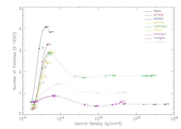
Figure 1: Total Baryon number, A, vs Central Density, $\rho{}_{\text{0}}$, of a self-gravitating sphere in hydrostatic equilibrium. These curves represent continuous sequences of the final results of integrations of Equation 4 using different central pressures as boundary conditions for the system of differential equations of structure. Each different line represents the choice of a different EOS. The asterisked points on the curves represent configurations corresponding to critical points of various quantities. The capital letters A, M, and R indicate local maxima of baryon number, mass, and radius, respectively, vs. $\rho{}_{\text{0}}$. Lower-case letters represent analogous local minima. The curves are drawn solid where our implementation of the Chandrasekhar stability theorem indicates that the solution corresponds to stable hydrostatic equilibrium. The curves are drawn as dotted lines where it indicates unstable hydrostatic equilibrium. HTWW showed that solutions lying to the left of the maximum on any particular curve shown here are stable, while solution lying to the right are unstable. Note the close agreement between these two independent methods of calculating stability.

We can also interpret the stable (solid-line) portion of each line as the construction, by slow mass accretion, of an object consistently obeying a single EOS, to the point of collapse. As long as material of the appropriate composition and temperature is added with negligible bulk kinetic energy at a rate negligible within a hydrodynamic timescale, a single object will move along a given line from left to right.

To continue moving the so-constructed object to the right, into and through the unstable portion, requires a different action. We see that the total mass of the object must decrease for a finite span, even as the central density increases. This means simply that we have reached the maximum possible mass that our chosen EOS can support, and to achieve any greater compression in the core of the object we must remove a quantity of matter while increasing that compression, or else the object will immediately collapse. (Note that this must be accomplished while somehow avoiding the introduction of the slightest hydrodynamic perturbation not orthogonal to an overall compression. No easy feat!) This technique will carry us to the first minimum of an EOS’s curve in Figure 1 after the first maximum. That family of solutions to the structure equation gives rise to Type I DBHs. Material can then be added as before, which will bring us to the second maximum, at a price of having to employ a still-more-sophisticated technique to avoid introducing catastrophic perturbations. However, as one might expect we can only return a very small fraction of the removed matter before reaching that second maximum. We must then remove material once again, and so on ad infinitum, in a strongly damped oscillation of baryon number with respect to central density. All of the configurations resulting from the latter manipulations correspond to the progenitors of Type II DBHs, though not as simple identifications, as with the Type I solutions.

Figure 2 is a similar graph of total mass as measured by an observer at infinity (the “Keplerian mass”) vs. central density. It shows some subtle but critical differences from Figure 2 that we will elaborate with the next figure. We include Figure 2 because the Keplerian mass is useful for comparisons to observations and the TOV limit for a given EOS may be found directly as the maximum of that EOS’s curve. The bold, red line indicates the mass of the neutron star observed by Demorest et al. (2010). Although some corrections beyond the scope of this work must be made for rotation, any EOS whose TOV limit falls below this line must be rejected as incorrect.

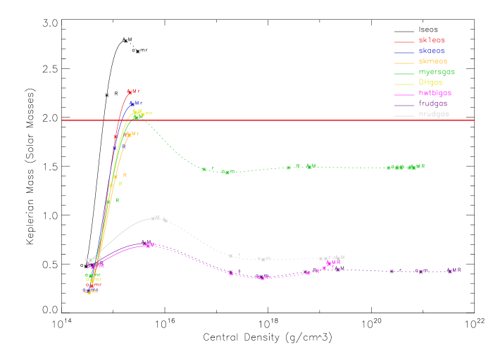
Figure 2: Keplerian Mass, M, vs. Central Density, $\rho{}_{\text{0}}$, of a self-gravitating sphere in hydrostatic equilibrium. These curves are drawn with the same conventions as those in Figure 1. This graph shows us the total mass of a sphere in hydrostatic equilbrium as measured by a very distant observer. The maximum of the frudgas curve (Fully Relativistic, UltraDegenerate GAS, the same EOS used by Oppenheimer and Volkoff (1939)), demonstrates that we have accurately reproduced the original, eponymous prediction of the TOV limit of 0.71 M_⊙. The bold, red line indicates the mass of the neutron star observed by Demorest et al. (2010). Modulo corrections due to rotation, any EOS whose maximum falls below this line must be rejected as incorrect.

We demonstrate the accuracy of our implementation of the stability criterion by comparing it to an independent method of calculating stability. This latter method (developed by HTWW, p. 50) is based on a group property of a family of spheres calculated with the same equation of state, but differing central densities. HTWW demonstrated that spheres with lower central densities, i.e. left of the baryon number maxima, denoted A in Figure 1, are in stable equilibrium and correspond to physical neutron stars, while those at higher central density to the right of the mass maxima are unstable. The close agreement between the family stability property (left of the mass maximum is stable, right is unstable) and the single-sphere, independent calculation of the Chandrasekhar stability criterion (whether the curve is solid or dashed) gives us great confidence in our interpretation and implementation of the latter.

5.3 The Fate of an Unstable Equilibrium Configuration

We know that unstable objects precisely at the TOV limit will collapse gravitationally rather than disassociate because no stable equilibrium configuration exists for that number of baryons, and no catastrophically exothermic physics comes into play with our EOSs in this regime. The fate of an unstable equilibrium configuration with central density greater than the TOV-limit (located to the right of the first maximum on each curve shown in Figures 1 and 2), however, is not predetermined.

Let us consider an informative merging of the previous two figures in order to make evident the differences between the two. The results are shown in Figure 3, where we have plotted the Keplerian mass of objects in equilibrium versus their baryon number, i.e., correlated values of the dependent variables of Figures 1 and 2. In addition to matching different variable values for particular configurations as above, using Equation 4 to calculate baryon number also allows us to link different configurations that correspond to rearrangements of the same amount of matter. Those relationships would otherwise be impossible to detect.

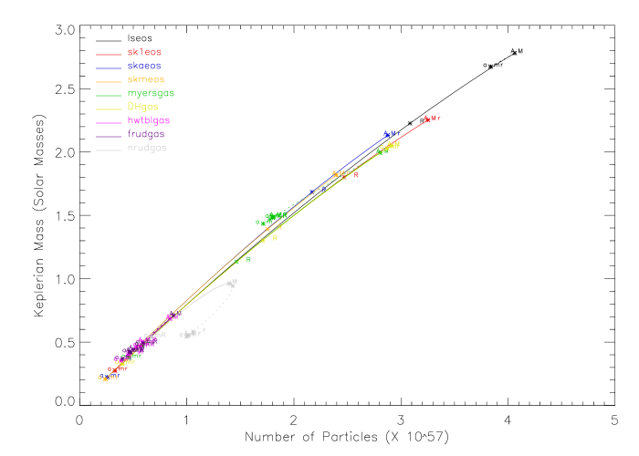
Figure 3: Keplerian Mass, M, vs Total Baryon Number, A, of a self-gravitating sphere in hydrostatic equilibrium. These curves are drawn with the same conventions as those in Figure 1. The vertical distance between the stable equilibrium branch (solid) and unstable equilibrium branch (dashed) of a given EOS for a given number of baryons is the mass equivalent of the PV work necessary to compress the stable equilibrium configuration to the verge of collapse. The non-relativistic EOS included as a test for consistency (nrudgas, see Section 3.7) is detected immediately as the one curve that takes a “wrong turn,” as its mass calculation includes rest mass and binding energy but assumes kinetic energy is negligible.

Note that the non-relativistic EOS (nrudgas, See Section 3.7) curve in Figure 3 shows two unique deviations from the behavior exhibited by the properly relativistic curves. The first deviation is that it takes a “wrong turn”- the unstable branch of the curve lies below the stable branch. This defect arises from the neglect of kinetic energy, which is significantly greater in an unstable configuration than the stable configuration of the same number of baryons, in the calculation of the Keplerian mass. The second defect is that while all the relativistic EOSs come to sharp points at the upper right, the non-relativistic EOS is rounded. The discontinuity of the parametric graph indicates that both the Keplerian mass and baryon number are stationary with respect to their underlying independent parameter, central pressure. The non-relativistic EOS’ rounded end indicates a defect in the calculation of the chemical potential, also traceable to the neglect of kinetic energy.

For clarity we extract one curve from Figure 3 and display it in Figure 4. Note that central density increases along the stable (solid line) portion of the curve from lower left to upper right, and then increases still more along the unstable (dotted line) portion of the curve. Due to the strongly damped oscillations in both baryon number and Keplerian mass, extending this curve (or any other curve from Figure 3) even to infinite central density would result in only a minute zig-zag pattern at the lower left of its unstable branch, terminating at a finite mass and baryon number barely distinguishable from the endpoint shown.

We can examine the compression process using the relationship between different configurations with the same baryon number as mentioned above. The vertical interval demarcated on Figure 4 is bounded by the stable and first unstable hydrostatic equilibrium configurations of the same baryon number for a given EOS. This vertical distance is the mass equivalent of the net work (Pressure-volume work minus gravitational potential energy released) required to compress the stable configuration to the point of gravitational collapse. One such relationship between an arbitrary stable configuration and the corresponding compressed, unstable configuration with the same baryon number is illustrated in Figure 4 with a bold vertical line.

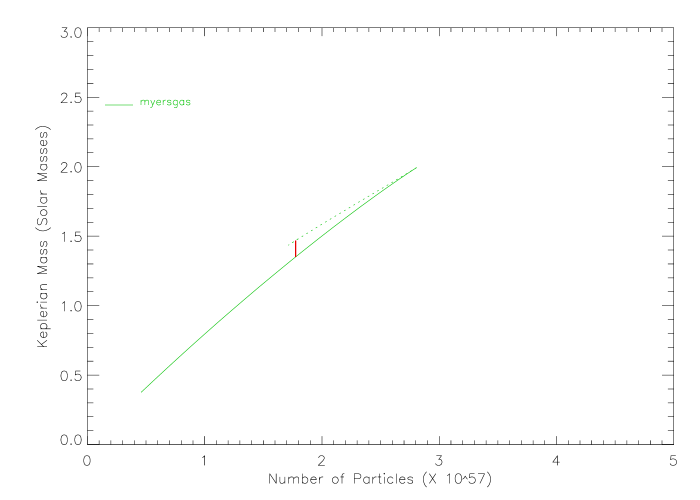
Figure 4: Keplerian Mass, M, vs. Total Baryon Number, A, of a self-gravitating sphere in hydrostatic equilibrium, excerpt. A single curve is extracted from Figure 3 in order to clarify discussion. The vertical interval highlighted in red on this figure marks the difference in mass between the stable and unstable equilibrium configurations of an arbitrary number of baryons. The energy equivalent of the mass difference is equal to the net work needed to compress the stable configuration into the unstable configuration.

Consider the process of quasistatically compressing an ensemble of matter from its stable hydrostatic equilibrium configuration to its second hydrostatic equilibrium, this one unstable. The equilibrium configurations at either end of the process must necessarily both have pressures that vanish approaching their surfaces. Otherwise, the finite outward pressure on the surface layer of the sphere would cause it to expand into the vaccuum immediately (i.e., not in response to a stochastic or microscopic perturbation), violating the definition of hydrostatic equilibrium. The intermediate configurations (same total baryon number and central density lying somewhere between the central densities of the equilibrium configurations), however, cannot possibly have pressures vanishing near their surfaces because these configurations are in equilibrium with the external force compressing the configuration. Figure 4 demonstrates that an initially constrained, intermediate configuration, once allowed to slowly relax and radiate mass-energy content, will come deterministically to rest by expanding to the stable equilibrium configuration.

A simple analogy for the behaviors just described is that of a boulder lying in a hilly region. A stable equilibrium configuration corresponds to a boulder location at the bottom of a valley. Any small amount of work done on it will displace the boulder from its original location. A force is then required to maintain the boulder’s displaced position, and if it is removed, the boulder will relax back to its initial location. A large amount of work done, however, can displace the boulder to the top of the nearest hill, from which it may return to its original position or roll down the other side of the hill, depending on the details of its perturbation from the top.

The boulder analogy highlights several important observations regarding self-gravitating spheres in hydrostatic equilibrium. The two equilibrium positions, stable and unstable, are self-contained in the sense that they require no containment pressure and therefore have a zero pressure boundary, corresponding to zero force required to maintain the boulder’s position at the top and bottom of the hill. In the intermediate positions, however, a containment pressure is required to maintain the structure of the sphere, just as a force is required to hold the boulder in place on the side of the hill. Because the containment pressure required to maintain or enhance the compression of the sphere is known to be zero at either equilibrium configuration, yet positive in between, continuity requires that there be a maximum containment pressure somewhere in the middle. Analogously, the hill must rise from a flat valley to a maximum steepness, then return to a flat hilltop.

Like a boulder at the top of a hill, once a self-gravitating sphere in hydrostatic equilibrium has been compressed from its stable equilibrium position to its first unstable equilibrium, it may follow one of two different paths depending on the details of its perturbation. The sphere will either gravitationally collapse or expand back to its stable configuration. All components of an evolving arbitrary perturbation corresponding to oscillatory eigenmodes will soon be negligible compared to the exponential growth eigenmodes. Moreover, unless the initial perturbation is fine-tuned, the fastest growing mode, i.e. the mode with the largest magnitude of frequency, is likely to soon dominate all other modes. In the case of self-gravitating, hydrostatic spheres, growth modes are determined by the sign of the square of their frequencies, so the largest (imaginary) frequency will correspond to the lowest (real) frequency squared- our fundamental mode, as discussed in Section 5.1. Recall that it is a pure expansion or contraction when that mode grows rather than oscillates, with no nodes except at the center, as required by symmetry. Whether the self-gravitating unstable hydrostatic sphere returns to its original, stable configuration or collapses most likely depends, then, solely on whether the initial phase of the “breathing” mode corresponds to a contraction or expansion.

In Figure 5, with vertical lines we show the change in radius necessary to bring two example configurations from stable to unstable equilibrium. We see that the softer EOSs such as HWTblGas require much greater compression than the stiffer EOSs, such as LS. We have drawn our comparisons at 0.7 and 3.9 x 10${}^{\text{57}}$ baryons, respectively. These baryon numbers are both 95% of the baryon number of the equilibrium configuration at the TOV limit for that EOS.

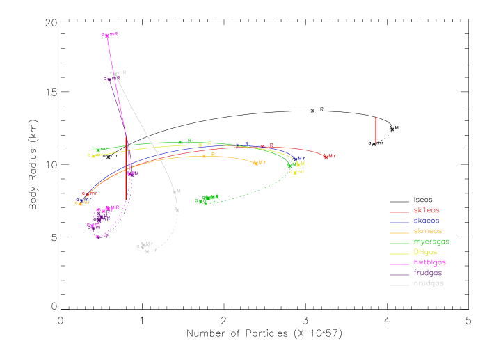
Figure 5: Radius, R vs. Baryon Number, A, of a self-gravitating sphere in hydrostatic equilibrium. In order to perturb a self-gravitating sphere in stable hydrostatic equilibrium, one must compress the sphere from the larger radius indicated by a solid curve vertically downwards to the corresponding unstable equilibrium point. Soft EOSs require much compression to go unstable. This is illustrated by the long vertical line connecting the stable configuration of 0.8 x 10${}^{\text{57}}$ baryons in the HWTblGas EOS to the unstable configuration of the same number of baryons in the same EOS. Stiff EOS require a much smaller change in radius. This is illustrated by the short vertical line connecting the stable and unstable configurations of 3.8 x 10${}^{\text{57}}$ baryons in the LS EOS. Both of these baryon numbers correspond to 95% of the baryon number of the configuration at the TOV limit.

5.4 Generalization of the Theorem

Chandrasekhar’s stability theorem as stated in HTWW has two limitations within which we must work: the theorem is only applicable to spheres, and it is assumed that those spheres are surrounded by vaccuum. Because gravity interferes only constructively, if a given sphere in hydrostatic equilibrium is unstable to gravitational collapse, then any arbitrary mass distribution containing a spherical region everywhere denser than that given sphere will also be gravitationally unstable. We implement this observation by considering only spherical regions excerpted from within computer simulation data sets in order to detect zones of gravitational collapse. We then estimate the mass contained within the spherical region as the lower limit of mass of a DBH formed from that zone of collapse. This only makes our criterion more conservative.

Because simulation data are very noisy, we are forced to take an average over angles for a given inscribed spherical region in a simulation data set. In Figure 6 we plot the density profile thus generated from a region we examined for instability. This procedure is discussed in more detail in Section 5.7. This approximation is not a strictly conservative assumption, so it may introduce false positives. These false positives may be weeded out by conducting a post-processing, ultra-high-resolution mini-simulation focused on the region in question, using the original data set as a spatial boundary condition throughout the mini-simulation.

In Figure 6 we show the region around the densest data point in the Fryer Type II supernova simulation data set. To generate this radial profile, all data points within 20 km are extracted and sorted by distance from the densest data point. The profile shown is roughly one half of a solar mass. Type I DBHs, with this EOS, are between 1.5 and 2 $M_{\odot}$, so this region is not a Type I DBH progenitor. Its central density also precludes it from being a Type II DBH progenitor, but that diagnosis is sensitive to the simulation’s spatial resolution at the center of the region. We discuss an avenue for detecting arbitrarily small, Type II DBHs in Sections 5.5 and 5.6.

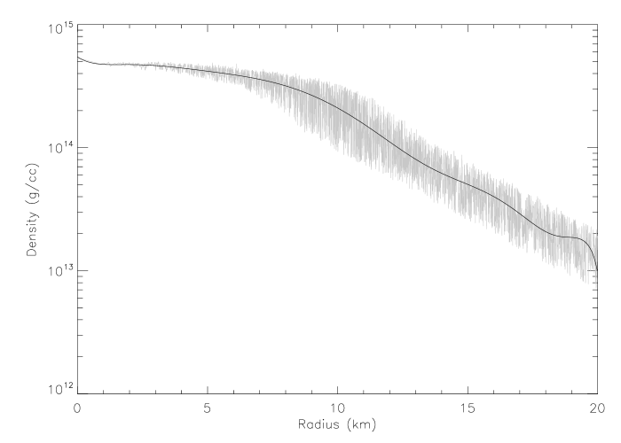
Figure 6: Radial Profile of a Typical Spherical Region Being Analyzed for Stability. This profile comes from the Fryer supernova simulation discussed in detail in Section 6.2. For economy, one out of every ten data points extracted from simulation data are shown plotted in gray. The tenth-order polynomial fit to the full ensemble of extracted data points is overplotted in black. This region comprises roughly one half of a solar mass. The Type I technique developed in this paper, with this EOS, can detect DBHs between 1.5 and 2 $M_{\odot}$, so this region is ruled out as a Type I DBH progenitor. We discusss the detection of Type II DBHs, which extend to arbitrarily small masses, in Sections 5.5 and 5.6.

To address the second limitation of Chandrasekhar’s stability theorem, the vaccuum boundary condition, we compare a non-vaccuum bounded spherical region extracted from a simulation data set to a vaccuum-bounded theoretical model sphere known to be unstable via Chandrasekhar’s theorem. Since gravity only constructively interferes, if the spherical region of data is everywhere denser than the unstable sphere, the spherical region will also be unstable.

5.5 Smaller-Still Dwarf Black Holes?

The work we have presented thus far deals with spherical configurations only so compacted as to have a single mode of instability. For very large baryon numbers, greater than the maxima shown in Figure 1, no stable equilibrium configuration exists- this is the familiar result that, above the very restrictive TOV limit of at most a few solar masses (Demorest et al., 2010), material can only be supported by an active engine in the interior (e.g. fusion, for stellar bodies), and when that engine shuts down, catastrophe ensues. Counterintuitively, there is also a minimum baryon number for finding an unstable equilibrium state in the manner previously described. For any given EOS, the first minimum in baryon number or Keplerian mass vs. central density after the maximum signifying the TOV limit is the absolute minimum for all higher central densities. The curves shown in Figures 1, 2, and 9, if extrapolated arbitrarily while maintaining constraints of physicality, would be characterized by damped oscillation in baryon number, mass, and radius, respectively, with increasing central density. For instance, from Figure 2, we can see for the Myers and Swiatecki EOS, no vaccuum-bounded, unstable configuration of mass 1 $M_{\odot}$ exists. Yet, if one slowly compresses a small amount of matter to an arbitrarily high pressure, a gravitational collapse must ensue sooner or later. What, then, does $\sim$1 $M_{\odot}$-worth of material look like, just before it is compressed to the point of gravitational collapse?

Since we have posited that the extreme DBH progenitors result from compressing a small amount of material, let us consider a small, isolated, hydrodynamically stable, static, spherical configuration of matter bounded by vaccuum. We then introduce outside that configuration (through sufficiently advanced technology) a rigid, impermeable, spherical membrane whose radius can be changed at will. If we gradually shrink the membrane, even to the verge of the gravitational collapse of its contents, then the configuration of matter inside must at all times obey Equations 1 and 2. This is because the interior layers of the matter inside the membrane are insensitive as to what is causing the layers above them to exert a particular inward pressure.

The structure equations are first order in $r$, so if two solutions are found with the same (central) boundary condition, they must be identical from the center to the radius of the membrane. The progenitors of extreme DBHs (when constructed quasi-statically), therefore, are truncated solutions of the structure equations, with central density high enough that the complete solution (out to sufficient radius for pressure and density to reach zero) would have two or more radial eigenmodes that grow rather than oscillate. In Table LABEL:tab:Mass-Range-Scenarios we have compiled the scenarios under which different amounts of matter would collapse, gravitationally.

Table 2: Mass Ranges of Qualitatively Different Gravitational Collapse Scenarios Any amount of matter is vulnerable to gravitational collapse if it becomes sufficiently dense. Different amounts of matter will exhibit qualitatively different gravitational collapse scenarios. The numerical figures of 3/2 and 2 M_⊙ are approximate and derived from the Myers and Swiatecki (1997) EOS and the Demorest et al. (2010) neutron star. That neutron star is assumed to be very near the TOV limit since it is so much more massive than any other yet observed. That EOS is chosen because its TOV limit is the closest to 2 M_⊙, and its first post-TOV-limit mass minimum gives rise to the 3/2 M_⊙ number.

Mass Range	Exemplar	Discussion
> 2 M⊙	Direct collapse without supernova of a very massive star	This mass range lies above the TOV limit of the real-world, universal EOS. There is no permanent equilibrium configuration for this amount of matter whatsoever. Thus it can only be supported in short-term hydrostatic equilibrium by an active (i.e., explicitly out of chemical- or other-equilibrium) engine consuming some sort of fuel on a longer characteristic time scale, such as fusion in massive stars or energy released by a black hole capturing matter, as in AGNs. When the fuel is expended, catastrophe will inevitably ensue.
2 M⊙	Collapse of accreting neutron star	This is the collapse of an object that has reached precisely the TOV limit by growing quasi-statically, as through slow accretion. Catastrophe ensues with the accretion of one more particle. The approximate value of this mass is taken from Demorest et al. (2010), assumed to be very near the TOV limit.
$\frac{3}{2}$ - 2 M⊙	Type I DBH formed in, perhaps, hypernova	A configuration of matter in this range will assume a stable equilibrium configuration. If it is then slowly compressed by exterior force, it will eventually reach a second equilibrium, this time unstable. As the configuration approaches that second equilibrium, the external, boundary pressure decreases, and vanishes entirely upon reaching it. It will collapse if perturbed in a manner dominated by compression, or expand to its stable equilibrium configuration if perturbed in a manner dominated by expansion. The limits of this mass range are defined by the region in which the curve of an assumed EOS decreases in Figure 2, to the right of the TOV limit. We give a value of $\frac{3}{2}$ M⊙ because that is the approximate limit corresponding to the myersgas EOS, the EOS we examined with a TOV limit closest to Demorest et al. (2010).
< $\frac{3}{2}$ M⊙	Type II DBH formed in, perhaps, SN Ia	A configuration of matter in this range will settle into a stable equilibrium configuration. It will exhibit no second, unstable equilibrium configuration, for any amount of compression it is forced to undergo. Instead, if compressed to the point of collapse, its core will commence doing so even while its upper layers continue to exert a pressure against the container compressing it.

To physically realize a truncated mathematical solution, we have no choice but to constrain a configuration with something functionally equivalent to the membrane of the above paragraphs. In the supernova simulations in which we would like to find extreme DBHs, this role would be fulfilled by turbulence or fallback driving mass collisions. In other words, the potentially unstable region is surrounded by high pressure gas acting to compress it.

Because they are truncated before the radius where pressure reaches zero, the progenitors of extreme DBHs will not appear in the figures depicting self-gravitating spheres in hydrostatic equilibrium, which have containment pressures of zero. As described in Section 5.3, the extreme DBH progenitor spheres would expand if the membrane (or, realistically, the surrounding gas) were withdrawn, but under the influence of the membrane they can achieve instability to gravitational collapse.

HTWW (p. 46) demonstrate that the zero-containment-pressure configurations lying in the first unstable region with increasing baryon number of Figure 1 have two growth eigenmodes. The second eigenmode will have a single node, and in the case of two growth eigenmodes, this enables the outer layers to expand while the inner layers contract catastrophically. This is the collapse scenario by which very small DBHs could form. Unfortunately, detecting this instability is a far less tractable problem than the work we have already presented, instabilities arising in zero-containment pressure configurations from the growth of the lowest eigenmode. It is less tractable because in order to reach a definite conclusion about stability we must be able to calculate the radius necessary to bring a Type II DBH progenitor to the brink of collapse, or equivalently, calculate where we must truncate a mathematical solution to the structure equations (1-5) in order to leave a configuration only marginally stable. In contrast, for Type I DBHs, the critical radius arises from the integration of the structure equations automatically.

The complete, equilibrium sphere solutions from which we obtained our truncated solutions lie to the right of the first unstable minimum in Figure 1. This location means that they have two or more eigenmodes of exponential growth. Our thought experiment of slowly compressing small amounts of matter, however, demonstrated that the truncated solutions, on the other hand, can have only a single mode of growth. That is the very criteria by which we decided to halt our thought-compression; we stopped as soon as the sphere became unstable to gravitational collapse, and that requires only a single growth mode (Section 5.1). We find, therefore, that truncating a solution apparently changes its eigenspectrum.

This may seem strange. Why shouldn’t the truncated, inner layers simply collapse in the same manner as the whole sphere would? How do the inner layers know and respond to the behavior (or even existence) of the upper layers? Considering the boundary condition resolves the puzzle. The untruncated solution can expand into the vaccuum in response to an outgoing perturbation, so the outer boundary condition is transmissive. The kinetic energy of the perturbation would be gradually converted to potential energy or radiated entirely. It could return to the center only as the entire sphere relaxed. The truncated solution, in contrast, is abutted by a physical obstacle that may reflect some perturbation. Some of the kinetic energy of a perturbation of such a sphere would rebound directly to the center. Just as in the simple classroom demonstration of changing the pitch of a pipe organ pipe by opening and closing its end, changing the boundary condition of a self-gravitating sphere changes its eigenspectrum. To detect these instabilities, we must decide where to truncate a solution so that it includes just enough material to be unstable. Our calculation to determine where to truncate follows in the next section.

5.6 Detecting Higher-Order Instabilities

The marginally stable progenitors of Type II DBHs have very high central densities. From Figure 1 we see that for the Myers and Swiatecki EOS, for instance, the onset of instability of a second mode (first minimum after first maximum) occurs at a central density roughly 30 times greater than the onset of instability of the first eigenmode (first maximum). For this EOS, these critical points are at central densities of   $\sim$10${}^{\text{17}}$ g cm${}^{\text{-3}}$ and $\sim$  3 $\times$ 10¹⁵ g cm${}^{\text{-3}}$, respectively. As will be discussed in more detail in Section 6.2, the highest density we have yet found in a simulation is   $\sim$7 $\times$ 10${}^{\text{14}}$ g cm${}^{\text{-3}}$. We are currently seeking data sets achieving higher densities. Happily, as shown in Figure 7, the radial profiles of Type II DBH progenitors are very sharply peaked. The required region of extreme, thus-far-unprecendented density may be very small indeed. The curve shown in this figure with the lowest central density is the first Type II DBH progenitor, i.e., the first hydrostatic sphere that has more than one growth eigenmode.

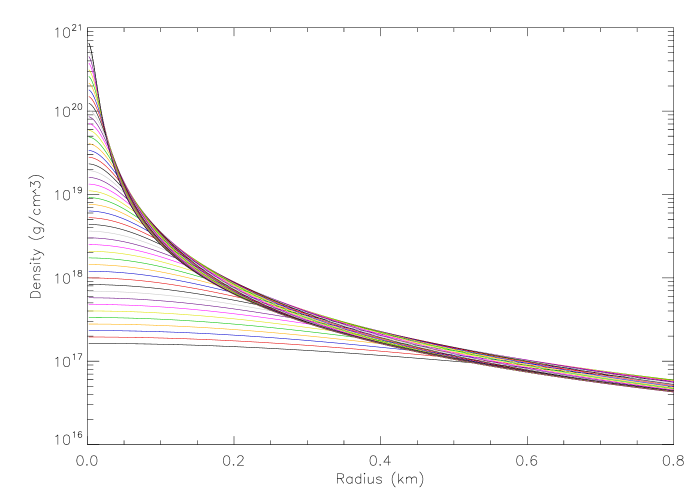
Figure 7: Central radial density profiles of extreme self-gravitating spheres in hydrostatic equilibrium. These curves, plotting the innermost regions of Type II DBH progenitors, show that these progenitors may not be detectable in simulation data at all unless the resolution is extremely fine, perhaps smaller than 100 m, because even the most and least extreme Type II DBH progenitors are nearly indistinguishable outside 600 m. The curve with lowest central density is the first Type II DBH progenitor, i.e., the first curve that, taken all the way to $P=0$, displays two or more modes of instability. This figure extrapolates the myersgas EOS much farther than it is intended to be taken, but any physically realistic EOS will display the same qualitative behavior.

In Figure 7 we see that the curves plotted that have the highest central density decrease in density by three orders of magnitude within roughly 200 m, and even the most and least extreme curves plotted on this chart are virtually indistinguishable outside 600 m. DBH progenitors have no chance at all of being resolved in a simulation data set except in regions where the spatial resolution is on the order of 100 m or less. In Figure 8 we plot the distance to the nearest neighboring data point for a sampling of data points in the Fryer Type II Supernova we analyzed. This simulation was conducted recently using the full computing resources of Los Alamos National Laboratory, yet even it achieves the necessary resolution only for a 10 km radius around its center of mass, or less.

Figure 8: Distance to Nearest Neighbor vs. Distance from Center of Mass for the Fryer Type II Supernova Simulation For economy we plot the distance to nearest neighbor for 1/10 of the data points in the Fryer data set. Figure 7 demonstrated the need for simulations of very high resolution, of order 100 m. Even with the computing resources available at Los Alamos National Laboratory that resolution is only found within $\sim$10 km of the center of mass of this simulation.

The high-central density termination point of the lseos, sk1eos, skaeos, skmeos, and DHgas curves in Figures 1, 2, 3, 4, and 5, are defined by the upper limits of published tables. In several of those cases we see very little of even the single growth-eigenmode regime, much less the two growth-eigenmode. (The myersgas, hwtbl, frudgas, and nrudgas EOSs are published or known in closed form and thus their curves are extended indefinitely, but in configurations with central densities much beyond roughly 8 $\times$ 10${}^{\text{14}}$ g cm${}^{\text{-3}}$, that is, twice nuclear density, these should be regarded as ambitious extrapolations suitable for illustrative purposes only.) For confidence in calculating the properties of DBH quasi-static progenitors, the upper limits of present EOSs must be extended.

Let us optimistically suppose some time in the future we will have an EOS reliably applicable to ambitious extremes, and that high-resolution, future supercomputer simulations of extreme phenomena reveal very high densities. How then should we proceed, i.e., could we generate some theoretical compressed and constrained configurations on the verge of higher-order acoustical collapse to compare to our hypothetical, hydrodynamic supercomputer simulation? This suggested procedure is in analogy to the algorithm discussed in Section 5.7, where theoretical curves describing Type I DBH progenitors are compared to spherical regions of existing simulation data.

We must conduct a thought experiment in order to discover more detail about the progenitors of Type II DBHs. For concreteness, let us use the myersgas EOS and assume it is absolutely accurate to all densities with infinite precision. Let us consider two ensembles of matter of slightly different total masses. Let both lie below the TOV limit, roughly 2 M_⊙, so a stable equilibrium configuration exists for both. Allow the more massive ensemble to come to hydrostatic equilibrium, and spherically compress the less massive ensemble through outside forces so that its central density is equal to the central density of the first ensemble. Because the structure differential equations governing hydrostatic equilibrium (Equations 1 and 2, along with their adjuncts, Equations 4 and 5) are first order (in radius) and we are maintaining equal (central) boundary conditions by fiat, both ensembles will have identical radial dependence of their physical quantities. The only difference between the two is that the more massive ensemble extends from $r=0$ to $R$, that is, the radius where pressure vanishes, while the less massive ensemble truncates at $r\lesssim R$, where pressure is still finite.

Let us then quasistatically compress both of our spherical ensembles, maintaining equal central density between the two. That central density will increase monotonically. The more massive ensemble will reach the verge of gravitational collapse first, while the less massive ensemble will need to be compressed to a slightly higher density to gravitationally collapse. Since we have made the masses of the two ensembles arbitrary apart from being below the TOV limit, we have proven the lemma that:

1. The central density of a static sphere on the verge of gravitational collapse increases monotonically as the total mass of the sphere decreases.

This statement applies to progenitors of both Type I and Type II DBHs. We already know the central density objects of roughly 2 M_⊙ down to 1.5 M_⊙ (in the myersgas EOS) on the verge of collapse (i.e., Type I DBH progenitors, which lie between the first maximum and following minimum on Figure 2 of a curve corresponding to a selected EOS) will have central densities of roughly 2 $\times$ 10${}^{\text{15}}$ erg cm${}^{\text{-3}}$ - 10${}^{\text{17}}$ erg cm${}^{\text{-3}}$, respectively. To look for objects of smaller mass on the verge of collapse, we must increase the central density even more.

2. A Type II DBH progenitor will have a central density greater than the minimum following the first maximum of an EOS’s curve as shown in Figure 2.

Type I DBH progenitors exert a vanishing pressure on their containers at the end of their compression because they are then identical to full, vaccuum-bounded solutions to the structure equations. If we look beyond central densities of 10${}^{\text{17}}$ erg cm${}^{\text{-3}}$ on Figure 2, however, the vaccuum-bounded solutions of the structure equations then commence increasing, while the mass of Type II DBH progenitors decrease, by construction. Nevertheless, since we arrived at these configurations by quasi-static compression, the Type II DBH progenitors must obey the structure equations. To reconcile this paradox, we have only one possible conclusion.

3. A Type II DBH progenitor is not described by the full, vaccuum-bounded solution of the structure equations with corresponding central density. It is a radial truncation of that solution at a smaller radius, where the pressure is still finite and the mass enclosed is less than the full solution.

Let us call the radius at which an ensemble reaches the verge of collapse the critical radius for that mass and baryon number. HTWW (p. 46) proved that the full, vaccuum-bounded solutions of the structure equations from which DBH progenitors are truncated have two or more growth eigenmodes. From our construction in the thought experiment, we dubbed a compressed sphere a DBH progenitor at the moment it acquired its first growth eigenmode. We could therefore discover the value of the critical radius for a particular central density by selecting different test radii at which to truncate that solution. We would then use a version of Chandrasekhar’s stability theorem (Equation 10) generalized to non-zero exterior boundary pressure to determine how many growth eigenmodes that truncation exhibits. The critical radius lies at the boundary between zero growth eigenmodes and one. Finally, repeating that procedure with structure equation solutions of many different central pressures would allow us to derive the relationships between other physical quantities of spheres on the verge of collapse such as total mass, exterior pressure, and density at the center and at the exterior boundary.

Unfortunately for us, Chandrasekhar’s derivation (Chandrasekhar, 1964), being a calculus of variations technique, necessarily assumes the existence of a node at the outer boundary of the spherical region to which it is applied and therefore inextricably assumes vanishing pressure at the outer radius of the body in question. However, since we have not yet discovered any regions within simulations dense enough to be comparable to the central density of Type II DBHs, we have concluded that deriving a generalization of Chandrasekhar’s theorem utilizing non-zero exterior pressure boundary conditions is unnecessary at this time.

5.7 The Algorithm for Finding Dwarf Black Holes

We summarize the results of our arguments for determining if there exists a region of matter in a spacelike slice of a general relativistic simulation that will collapse into a DBH as follows:

1. Find the densest data point inside a computational simulation of an extreme phenomenon (e.g. supernovae as described above) and take a spherical “scoop” out of the data centered on the densest point. For guidance on the size of scoops to remove, we can consult Figure 9. For a given EOS, the size of the scoops we need examine are limited to the range of radii from the radius of spheres at the onset on instability, i.e. the junction between solid and dashed curves, and the radius of spheres with central density equal to the highest single data point in the simulation data set.

   

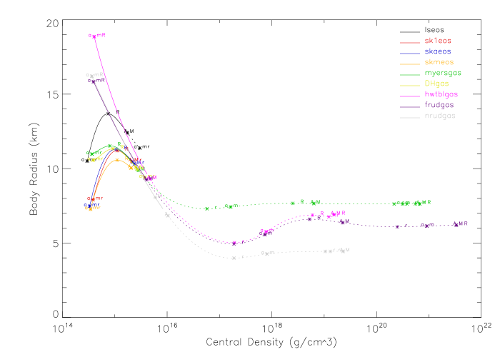
   Figure 9: Radius, R, vs Central Density, $\rho{}_{\text{0}}$, of a self-gravitating sphere in hydrostatic equilibrium. These curves are drawn with the same conventions as those in Figure 1. We can observe quantitatively the effects of having a “stiff” equation of state. Those EOSs that lead to a large estimate for the TOV limit also lead to an increase in radius with increasing $\rho{}_{\text{0}}$ before the final decrease in radius approaching the onset of instability. “Soft” equations of state lead to monotonic decreases in radius as $\rho{}_{\text{0}}$ increases from the lower limit of this figure to the onset of instability. The high central density limits of the lseos, sk1eos, skaeos, skmeos, and DHgas are defined by the upper limits of their published tables. The other curves are known in closed form and are thus extended indefinitely, but beyond roughly twice nuclear density these data points should be considered for illustrative purposes only.

2. Construct a sphere in hydrostatic equilibrium according to the structure equations tailored to match the physical properties of the scoop as closely as possible. The central pressure of the theoretical sphere is set equal to the central pressure of the data scoop. The temperature and other “$X$” thermodynamic variables are, as functions of $r$, fitted to the radial profile of the data scoop. Our experience with supernova simulation data sets reveals that this radial profile is quite noisy, so we make a tenth-order polynomial least-squares fit for each $X$ parameter for each scoop using IDL’s poly_fit routine.

3. Calculate the stability of the tailored hydrostatic sphere using Chandrasekhar’s theorem as described in Sections 5.3 and 5.4 for Type I DBHs and in Sections 5.5 and 5.6 for Type II DBHs. Proceed only if it is unstable.

4. Compare the tailored, unstable hydrostatic sphere to the scoop. If the scoop is everywhere denser than the sphere, it follows that the scoop should also be unstable to gravitational collapse. If the scoop is denser than the sphere only for an interior fraction of the sphere’s radius, then the scoop may still be unstable, as per our discussion in Sections 5.5 and 5.6. For this to occur, the sphere must be dense enough to exhibit at least two growth eigenmodes, i.e., two negative eigenvalues of oscillation frequency squared. Conveniently, the algorithm we use for calculating eigenvalues returns all of them simultaneously, so we have the second eigenvalue ready at hand. We have not yet found any simulations where this scenario comes into play.

5. Determine the total mass of the scoop inside the radius of the tailored, unstable hydrostatic sphere, and include it in the mass spectrum of black holes produced in this simulation.

6. Repeat these steps, through scoops of descending central density, until the pressure at the center of a scoop is less than the lowest central density necessary to achieve instability. That density is the central density of the sphere of mass equal to exactly the TOV-limit. This is a purely conservative assumption. Larger spheres with lower maximum densities also can achieve instability to gravitational collapse, but are not equilibrated, so we have no mathematical tools to prove that they are unstable, other than a direct comparison to the Schwarzschild radius for that amount of matter or the execution of a detailed hydrodynamic simulation.

6 Applications

6.1 Discussion

We are acquiring and testing simulation data of various extreme astrophysical phenomena from different research groups. For best results, it is desirable to employ the same EOS when constructing a tailored, unstable sphere as was used in constructing the “scoop” of simulation data (as described in Section 5.7) to which it will be compared. Due to the constantly evolving and patchwork nature of EOSes implemented in real-world simulations, this is not always possible, however. We have already completed the analysis of one simulation data set, a three dimensional, Type II supernova simulation provided to us by Chris Fryer of Los Alamos National Laboratory.

6.2 Type II Supernova

In order to determine whether a simulation has sufficient spatial resolution to detect DBHs, we consult Figure 10, which shows the radii of unstable spheres in hydrostatic equilibrium as a function of Keplerian Mass. The $R$ vs. $M$ relation is also critical to observational investigations of extreme phenomena, especially neutron stars, as probes of the extreme EOSs. The simulation conducted by Chris Fryer of the Los Alamos National Laboratory is fully three-dimensional, and it easily has fine enough spatial resolution, especially in the densest regions near the surface of the central proto-neutron star.

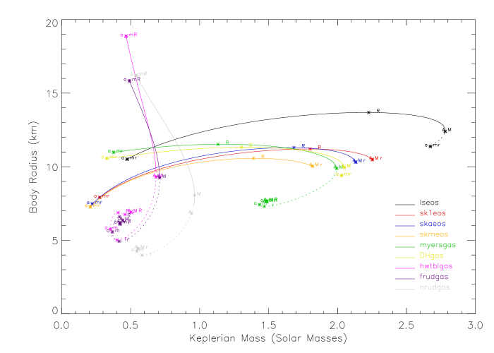
Figure 10: Radius, R, vs. Keplerian Mass, M, of a self-gravitating sphere in hydrostatic equilibrium. This graph gives a minimum estimate of the spatial resolution necessary for accurately detecting DBHs of a given mass in a simulation data set.

Fryer’s simulation uses the SK1 EOS from the Lattimer-Swesty quartet described in Section 3.6. This simulation was evolved from the canonical 23 M_⊙ progenitor developed by Young and Arnett (2005) using a discrete ordinates, smooth particle hydrodynamics code. The progenitor code, TYCHO, is a “One-dimensional stellar evolution and hydrodynamics code” that “uses an adaptable set of reaction networks, which are constructed automatically from rate tables given a list of desired nuclei.” (Young and Arnett, 2005) The TYCHO code is “evolving away from the classic technique (mixing-length theory) of modeling convection to a more realistic algorithm based on multidimensional studies of convection in the progenitor star.” (Fryer and Young, 2007) Fryer’s supernova simulation is described in more detail in Fryer and Young (2007), particularly Section 2 of that paper.

The maximum density found in this simulation was 6.95 $\times$ 10${}^{\text{14}}$ g cm${}^{\text{-3}}$, while the minimum density necessary to create a sphere in unstable equilibrium in this EOS is 2-3 $\times$ 10${}^{\text{15}}$ g cm${}^{\text{-3}}$. We do not have firm grounds on which to predict the creation of dwarf black holes from Type II supernovae, but being within a factor of 3-4 of the necessary density in one of the milder members of the menagerie of extreme astrophysical phenomena suggested we publish these results and proceed with investigating other supernova simulations and simulations of other phenomena.

6.3 Other Applications

We are currently seeking data sets from other simulations to analyze for possible DBH formation. One type of simulation in which we are interested is those with large total mass, such as the death of very massive stars or phenomena larger than stellar scale. We feel that those types of simulation supply the best arena for the Type I (i.e., the most massive, least dense) DBHs to arise, as even a single specimen of that end of the DBH spectrum would comprise a significant fraction (or all!) of the ejecta from small-scale events. We are also interested in smaller scale but extremely violent simulations, such as the explosive collapse of a white dwarf or neutron star, or compact object mergers, as these may give rise to the extremely high densities necessary for Type II DBHs to form, even though they probably do not have enough total mass involved in the event to create Type I DBHs.

Hypernovae, for instance, are a promising candidate for observing Type I DBHs. In addition to the especially large amount of energy released, hypernovae also occur in the context of very large ensembles of matter, the better for carving off into somewhat subsolar mass chunks. A recent study (Fryer et al., 2006) examined the collapse and subsequent explosion of 23 $M{}_{\odot}$ and 40 $M{}_{\odot}$ progenitors. While this physical phenomenon may be a promising candidate in the search for DBHs, the particular assumptions used by this group to render the calculation tractable, while fully valid for their intended research purposes, make it unlikely that we would find any DBHs in their simulation of it.

First, their study was one-dimensional, thus precluding a detailed treatment of aspherical phenomena including localized clumping into DBHs. They also treat the densest regions of the simulation as a black box with an artificially prescribed behavior, furthermore assumed to be neutrino-neutral. Details critical to the formation of DBHs may have been lost here. From Fryer et al. (2006):

We follow the evolution from collapse of the entire star through the bounce and stall of the shock... At the end of this phase, the proto–neutron stars of the 23 and 40 M_⊙ stars have reached masses of 1.37 and 1.85 M_⊙, respectively.

At this point in the simulation, we remove the neutron star core and drive an explosion by artificially heating the 15 zones ($\sim$3 × 10${}^{\text{-2}}$ M_⊙) just above the proto–neutron star. The amount and duration of the heating is altered to achieve the desired explosion energy, where explosion energy is defined as the total final kinetic energy of the ejecta (see Table 1 for details). The neutron star is modeled as a hard surface with no neutrino emission. Our artificial heating is set to mimic the effects of neutrino heating, but it does not alter the electron fraction as neutrinos would. The exact electron fraction in the ejecta is difficult to determine without multidimensional simulations with accurate neutrino transport. Given this persistent uncertainty, we instead assume the electron fraction of the collapsing material is set to its initial value (near Ye = 0.5 for most of the ejecta).

In addition, the very material most critical in generating DBHs plays no role in their investigation. Again, from Fryer et al. (2006):

As this material falls back onto the neutron star its density increases. When the density of a fallback zone rises above 5 × 10${}^{\text{8}}$ g cm${}^{\text{-3}}$, we assume that neutrino cooling will quickly cause this material to accrete onto the neutron star, and we remove the zone from the calculation (adding its mass to the neutron star).

They conclude their discussion with a very nearly prescient warning to a reader interested in DBHs:

Be aware that even if no gamma-ray burst is produced, much of this material need not accrete onto the neutron star. Especially if this material has angular momentum, it is likely that some of it will be ejected in a second explosion. (In a case with no GRB this will presumably be due to a similar mechanism, but without the very high Lorentz factors.) This ejecta is a site of heavy element production (Fryer et al. 2006). As we focus here only on the explosive nucleosynthesis, we do not discuss this ejecta further.

We are interested in the results of an updated study focused more on the dynamics and/or ejecta of the supernova explosion and less on nucleosynthetic yields, or one that preserved more of the information that was irrelevant to Fryer, Young, and Hungerford’s investigation.

7 Conclusions

We have proposed that a variety of extreme astrophysical phenomena, some newly recognized to be more turbulent and aspherical than previously appreciated, may compress local density concentrations beyond their points of gravitational instability. Upon gravitational collapse and expulsion, these local concentrations would become dwarf black holes (DBH). We expect that, due to the enormous velocities with which e.g. supernova ejecta is expelled, many or most DBHs may not be bound in galaxies but will instead be found in the intergalactic medium. As such, DBHs would not be subject to the constraints placed upon the abundance of Massive Astrophysical Compact Halo Objects (MACHOs) by observational searches for microlensing events in the halo of the Milky Way and its immediate neighbors.

We developed a heuristic for detecting regions within data sets of simulations of extreme astrophysical phenomena that are gravitationally unstable. In this investigation, it was revealed that the marginally stable objects that collapse into DBHs exhibit two qualitatively different collapse scenarios depending on the mass of the DBH progenitor. We termed DBHs whose progenitor fell into the more massive scenario Type I and those whose progenitor fell into the low mass scenario Type II. Type I DBH progenitors exhibit vanishing pressure on their surroundings before collapse, and therefore can be treated fully by our adaptation of the Chandrasekhar stability criterion. Type II DBH progenitors exhibit finite pressure on their surroundings before collapse, and thus cannot be fully treated by the Chandrasekhar stability criterion. At the present time we can merely rule out the presence of Type II DBH progenitors in a given, hypothetical data set only insofar as no data points exhibit densities as high as the central density of the least extreme DBH progenitor as shown in Figure 7. Due to the extremely small length scale of the core of a Type II DBH progenitor, however, we should not consider the lack of evidence for Type II DBHs in a data set to be completely conclusive. Sub-mesh scale dynamics could in theory create the very small but very dense regions that are necessary for Type II DBH progenitors but which are invisible in the data set.

We analyzed a data set from a Type II supernova simulation conducted by Christopher L. Fryer of Los Alamos National Laboratory and Patrick A. Young of Arizona State University for the presence of DBH progenitors. We found local density concentrations within a factor of 3-4 of both the minimum mass and density necessary to create Type I DBHs. We did not find any evidence of the densities necessary to create Type II DBHs, although the simulation had sufficient resolution to detect even the largest, most massive, and therefore least dense progenitors (if they were there) for only a few tens of kilometers around its center of mass.

Being within an order of magnitude of the conditions necessary for the creation of DBHs within one of the milder members of the menagerie of extreme astrophysical phenomena leads us to publish this work and seek data sets of simulations of any highly energetic astrophysical phenomena.

8 Acknowledgements

This research was made possible in part by a grant from the Maine Space Grant Consortium, two Frank H. Todd scholarships, and a Summer Graduate Research Fellowship and University Graduate Research Assistantship from the University of Maine. The authors would like to thank Chris Fryer of Los Alamos National Laboratory and Patrick Young of Arizona State University for their invaluable data set. Andrew Hayes would like to thank my wife Kate and daughter Evangeline for my entire universe.

References

- Alcock et al. (1996) Alcock, C. et al. 1996, ApJ, 471, 774
- Alcock et al. (1998) Alcock, C. et al. 1998, ApJ, 499, L9
- Bashforth and Adams (1883) Bashforth, F. & Adams, J. C., 1883, An Attempt to test the Theories of Capillary Action by comparing the theoretical and measured forms of drops of fluid. With an explanation of the method of integration employed in constructing the tables which give the theoretical forms of such drops, (Cambridge University Press)
- Burrows et al. (1995) Burrows, A., Hayes, J. & Fryxell, B., 1995, ApJ, 450, 830
- Carney and Latham (1987) Carney, B. W., Latham, D.W., 1987, Proc. IAU Symp., 117, 39C
- Chandrasekhar (1932) Chandrasekhar, S., 1932, ZA, 5, 321
- Chandrasekhar (1964) Chandrasekhar, S., 1964, PRL, 12, 114–116
- Demorest et al. (2010) Demorest, P. B., et al., 2010, Nature, 467, 1081–1083
- Douchin and Haensel (2001) Douchin, F. & Haensel, P., 2001, A&A, 380, 151-167
- Freese et al. (2000) Freese, K., Fields, B., & Graff, D., 2000, Nuclear Physics B Proceedings Supplements, 80, C305
- Friedland and Gruzinov (2006) Friedland, A. & Gruzinov, A., 2006, arXiv:astro-ph/0607244
- Fryer and Young (2007) Fryer, C. & Young, P., 2007, ApJ, 659, 1438-1448
- Fryer et al. (2006) Fryer, C., Young, P., & Hungerford, A., 2006, ApJ, 650, 1028-1047
- Fryer and Warren (2002) Fryer, C. & Warren, M., 2002, ApJ, 574, L65-L68
- Harrison et al. (1958) B. K. Harrison, M. Wakano, and J. A. Wheeler, 1958, in Onzieme Conseil de Physique Solvay, La Structure el l’evolution de l’univers, (Stoops, Brussels)
- Harrison et al. (1965) Harrison, B. K., Thorne, K. S., Wakano, M., & Wheeler, J. A., Gravitation Theory and Gravitational Collapse (1965, University of Chicago Press)
- Hawking (1974) Hawking, S. W., 1974, Nature, 248, 30-38
- Jeans (1902) Jeans, J., 1902, Philosophical Transactions, 199-A, 312
- Kippenhahn and Weigert (1994) Kippenhahn, R., & Weigert, A., 1994, Stellar Structure and Evolution (Springer)