Spin diffusion in $n$-type (111) GaAs quantum wells

Abstract

We utilize the kinetic spin Bloch equation approach to investigate the steady-state spin diffusion in $n$-type (111) GaAs quantum wells, where the in-plane components of the Dresselhaus spin-orbit coupling term and the Rashba term can be partially canceled by each other. A peak of the spin diffusion length due to the cancellation is predicted in the perpendicular electric field dependence. It is shown that the spin diffusion length around the peak can be markedly controlled via temperature and doping. When the electron gas enters into the degenerate regime, the electron density also leads to observable influence on the spin diffusion in the strong cancellation regime. Furthermore, we find that the spin diffusion always presents strong anisotropy with respect to the direction of the injected spin polarization. The anisotropic spin diffusion depends on whether the electric field is far away from or in the strong cancellation regime.

I INTRODUCTION

The spintronics with the aim to incorporate the spin freedom of the electrons to the traditional electronic devices to design novel devices has attracted much attention in the past decades.opticalorientation ; Awschalom ; Zutic ; Glazov ; Chen ; wuReview ; Korn ; Wolf For the application of such spintronic devices, the suitable spin relaxation time and spin diffusion/injection length are of essential importance,Tombros ; DattaDas ; Wunderlich ; Koo which requires comprehensive investigation for the thorough understanding of the spin properties in these systems. Actually, the spin relaxation and spin diffusion/injection have been widely investigated both experimentally and theoretically for a long period. opticalorientation ; wuReview ; Glazov ; Zutic ; Chen ; Awschalom ; Korn ; Wolf

In $n$-type III-V zinc-blende semiconductors, the D’yakonov-Perel’ (DP) mechanism,Dyakonov which results from the spin precession under the momentum-dependent effective magnetic field (inhomogeneous broadeningwu ) together with any scattering process, is identified as the predominant spin relaxation mechanism.Awschalom ; wuReview ; jiang ; jiang2 In the absence of the external magnetic field, the inhomogeneous broadening is mainly supplied by the spin-orbit couplings composed of the Dresselhaus termDresselhaus and the Rashba one.Rashba While the former one is due to the bulk inversion asymmetry of the crystal, the latter one originates from the structure inversion asymmetry and is tunable, e.g., via the electric field along the growth direction. The spin manipulation based on the competition of the Dresselhaus and Rashba spin orbit couplings is an interesting issue in semiconductor spintronics.Averkiev ; Schliemann ; Cheng2 ; Zarbo ; Sun ; Cartoixa ; Vurgaftman In the previous works, it was shown that the electron spin relaxation time in $n$-type (111) GaAs quantum wells (QWs) can be significantly enhanced when the in-plane components of the Dresselhaus term in the vicinity of the Fermi surface are strongly canceled by the Rashba term.Sun ; Cartoixa ; Vurgaftman This suggests the intriguing spin diffusion property in this system, which is however still not very clear, to our best knowledge. Therefore, the goal of this paper is to supply more knowledge for the spin diffusion in (111) GaAs QWs.

Differing from the spin relaxation in time domain, the inhomogeneous broadening in spin diffusion is determined by ${\mbox{\boldmath$\omega$\unboldmath}_{\bf k}}=m^{\ast}[{\bf\Omega}({\bf k})+g\mu_{B}{\bf B}]/k_{x}$,Cheng where ${\bf\Omega}$ and ${\bf B}$ are the spin-orbit coupling and external magnetic field, respectively. According to the previous works, the spin diffusion properties are strongly dependent on the detailed form of the inhomogeneous broadening. Specifically, in $n$-type (001) GaAs QWs where the inhomogeneous broadening is introduced by Dresselhaus spin-orbit coupling, Cheng et al.Cheng showed that the spin diffusion is enhanced by the scattering but suppressed with the increase of the temperature in the strong scattering regime. In contrast, the spin diffusion length is reduced by increasing the scattering strength when the scattering is rather weak. For the inhomogeneous broadening supplied solely by the external magnetic field in Si/SiGe QWs, Zhang and WuZhang found that the spin diffusion is suppressed by scattering monotonically. Interestingly, the spin diffusion length is reduced by the scattering in the weak scattering regime and turns to be a constant in the strong scattering limit (independent of the electron density, temperature, and scattering strength) in the monolayer graphene, where the Rashba spin-orbit coupling is dominant.Zhanggraphene Due to the partial cancellation between the Dresselhaus and Rashba terms, the influence of the electron density, temperature, and scattering strength on the spin diffusion length in $n$-type (111) GaAs QWs is expected to be an interesting issue.

In the present paper, we investigate the steady-state spin diffusion in $n$-type (111) GaAs QWs by solving the kinetic spin Bloch equations (KSBEs),wuReview which include all the relevant scatterings, i.e., electron-impurity, electron-acoustic/longitudinal-optical-phonon, and electron-electron scatterings. This work only focuses on the DP-limited spin relaxation in the strong scattering regime. We find that the electric field (along the growth direction) dependence of the spin diffusion length shows a peak due to the strong cancellation between the Dresselhaus and Rashba spin-orbit couplings. We find that the spin diffusion length, out of the strong cancellation regime, is insensitive to the temperature, doping density and electron density. However, the spin diffusion length is markedly manipulated by changing temperature and doping density around the peak. For the degenerate electron gas, the electron density can also lead to observable influence on the spin diffusion length. Last but not the least, we investigate the anisotropy of the spin diffusion with respect to the spin polarization direction of the injected electrons. The analytical solution of the KSBEs with only electron-impurity scattering is also presented to explain the numerical calculation.

This paper is organized as follows. In Sec. ii@, we introduce the KSBEs and give an analytical investigation for the case with only the electron-impurity scattering. In Sec. iii@, the spin diffusion is investigated by solving the KSBEs numerically with all the relevant scatterings included. A brief summary is given in Sec. iv@.

II KSBEs AND THE ANALYTICAL INVESTIGATION

We start our investigation from $n$-type (111) GaAs QWs under the infinite-depth-square-well approximation. The well width $a$ is taken to be 7.5 nm and only the lowest subband is relevant in our investigation. The electrons with their spins polarized along the direction ${\bf\hat{n}}$ are injected into the QWs at the left boundary ($x=0$) and diffuse along the $x$-axis. The right boundary is set to be $x=L$ with $L$ much longer than the spin diffusion distance. Therefore, the spin polarization of the electrons at the right boundary is always set to be zero. Since no magnetic field is applied in our model, the spinors precess only due to the DP term. Setting the $z$-axis along the growth direction [111], $x$-axis along [1$\bar{1}$0] and $y$-axis along [11$\bar{2}$], the total DP term reads

$$\begin{cases}\Omega_{x}({\bf k})=\gamma({-k^{2}+4{\langle k_{z}^{2}\rangle}})k_{y}/{2\sqrt{3}}-\alpha eE_{z}k_{y},\\ \Omega_{y}({\bf k})=-\gamma({-k^{2}+4{\langle k_{z}^{2}\rangle}})k_{x}/{2\sqrt{3}}+\alpha eE_{z}k_{x},\\ \Omega_{z}({\bf k})=\gamma({k_{x}^{3}-3k_{x}k_{y}^{2}})/\sqrt{6}.\end{cases}$$ (1)

Here, $\gamma$ and $\alpha$ are the Dresselhaus and Rashba spin-orbit coupling coefficients, respectively. $E_{z}$ stands for the electric field along $z$-axis and ${\langle k_{z}^{2}\rangle}=(\pi/a)^{2}$ is the average of the operator $-(\partial/\partial z)^{2}$ over the electron state of the lowest subband. It is clear that for the particular electric field

$$E^{c}_{z}=(4{\langle k^{2}_{z}\rangle}-\overline{k^{2}})\gamma/(2\sqrt{3}\alpha e),$$ (2)

the in-plane components of the Dresselhaus spin-orbit coupling are strongly canceled by the Rashba term.Cartoixa ; Vurgaftman ; Sun $\overline{k^{2}}$ here is the average of $k^{2}$ over the imbalance of the spin-up and -down electrons.

The KSBEs readwuReview ; wu

$$\partial_{t}{\rho_{\bf k}(x,t)}=-{e}{\partial_{x}\Psi(x,t)}{\partial_{k_{x}}\rho_{\bf k}(x,t)}-({k_{x}}/{m^{\ast}}){\partial_{x}\rho_{\bf k}(x,t)}$$

$$\hskip 22.76228pt\mbox{}+{\partial_{t}\rho_{\bf k}(x,t)}\big{|}_{\mbox{coh}}+{\partial_{t}\rho_{\bf k}(x,t)}\big{|}_{\mbox{scat}}.$$ (3)

Here, $\rho_{\bf k}(x,t)$ are the single-particle density matrices of electrons with the in-plane wave-vector ${\bf k}$ at position $x$ and time $t$. $m^{\ast}$ is the effective mass. $\Psi(x,t)$ is the electric potential satisfying the Poisson equation $\nabla^{2}_{x}\Psi(x,t)=e[N_{e}(x,t)-N_{0}]/(a\kappa_{0}\varepsilon_{0})$ with $N_{e}(x,t)=\sum_{\bf k}{\rm Tr}[\rho_{\bf k}(x,t)]$ standing for the local electron density. $N_{0}$ is the background positive charge density and $N_{e}(x,0)=N_{0}$ denoting the initial condition. $\varepsilon_{0}$ and $\kappa_{0}$ are the vacuum and relative static dielectric constants, respectively. ${\partial_{t}\rho_{\bf k}(x,t)}\big{|}_{\mbox{coh}}=-{i}[{\mbox{\boldmath$\Omega$\unboldmath}}({\bf k})\cdot{\mbox{\boldmath$\sigma$\unboldmath}}/2+\Sigma_{\bf k}(x,t),\rho_{\bf k}(x,t)]$ is the coherent term with $\Sigma_{\bf k}(x,t)=-\sum_{\bf q}V_{q}\rho_{{\bf k}-{\bf q}}(x,t)$ being the Hartree-Fock term.Haug Here, $\sigma$ are the Pauli matrices and $V_{q}$ is the Coulomb potential within the random phase approximation.Zhou The scattering term ${\partial_{t}\rho_{\bf k}(x,t)}\big{|}_{\mbox{scat}}$ includes the electron-impurity, electron-acoustic/longitudinal-optical-phonon, and electron-electron scatterings, of which the expressions can be found in Refs. Zhou, and weng, .

To speculate the properties of the spin diffusion, we first simplify the KSBEs with only the elastic impurity scattering included in the scattering term. Then, by taking the steady-state condition, i.e., $\partial_{t}{\rho_{\bf k}(x,t)}=0$, and performing the Fourier transformation with respect to $\theta_{\bf k}$ [with ${\bf k}=k(\cos\theta_{\bf k},\sin\theta_{\bf k})$], one obtains

$$\partial_{x}(\rho^{l+1}_{k}+\rho^{l-1}_{k}) = -{2}{\rho^{l}_{k}}{/({v_{k}}\tau^{l}_{k})}-\gamma_{k}[\sigma_{z},\rho^{l-3}_{k}+\rho^{l+3}_{k}]$$ (4)

$$\mbox{}-\beta_{k}[\sigma_{+},\rho^{l+1}_{k}]+\beta_{k}[\sigma_{-},\rho^{l-1}_{k}],$$

where $\sigma_{\pm}=(\sigma_{x}\pm i\sigma_{y})/2$, $v_{k}=\frac{k}{m^{\ast}}$, $\beta_{k}=m^{\ast}[{\gamma({k^{2}-4{\langle k_{z}^{2}\rangle}})/{2\sqrt{3}}+\alpha eE_{z}}]/2$, $\gamma_{k}=i\gamma k^{2}m^{\ast}/(2\sqrt{6})$, and $\rho^{l}_{k}=\frac{1}{2\pi}\int^{2\pi}_{0}d\theta_{\bf k}\rho_{\bf k}e^{-il\theta_{\bf k}}$. Here, $1/\tau^{l}_{k}=m^{\ast}N_{i}\int^{2\pi}_{0}d\theta_{\bf k}[1-\cos(l\theta_{\bf k})]U^{2}_{\bf q}/(2\pi)$ is the $l$th-order momentum-relaxation rate. $N_{i}$ stands for the bulk impurity density and $U^{2}_{\bf q}=\int^{\infty}_{-\infty}\frac{dq_{z}}{2\pi}|\frac{e^{2}}{\epsilon(q)(q^{2}+q^{2}_{z})}|^{2}|I(iq_{z})|^{2}$ is the impurity scattering potential with $|{\bf q}|=\sqrt{2k^{2}(1-\cos\theta_{\bf k})}$. $\epsilon(q)$ and the $I(iq_{z})$ are the screening functionZhou and form factor,weng respectively. In the strong scattering limit, the electron distribution approaches isotropy in the momentum space. Therefore, one can involve only the lowest two orders of $|l|$ ($=0$, 1) and obtainZhanggraphene ; Zhang

$$\partial^{2}_{x}\rho^{0}_{k}= -2i\beta_{k}[\sigma_{y},\partial_{x}\rho^{0}_{k}]+\beta^{2}_{k}[\sigma_{x},[\sigma_{x},\rho^{0}_{k}]]$$ (5)

$$\mbox{}+\beta^{2}_{k}[\sigma_{y},[\sigma_{y},\rho^{0}_{k}]].$$

The steady-state spin vector ${\bf S}^{0}_{k}(x)=\mbox{Tr}[\rho^{0}_{k}(x){\mbox{\boldmath$\sigma$\unboldmath}}]$ then can be obtained from Eq. (5) together with the boundary conditions ${\bf S}^{0}_{k}(0)={\bf S}^{0}_{k}$ and ${\bf S}^{0}_{k}(\infty)=0$. Obviously, ${\bf S}^{0}_{k}$ are determined by not only the spin polarization at the left boundary but also the electron density and temperature. (i) For the injected electrons polarized along the $x$-axis, i.e., ${\bf S}^{0}_{k}=(S^{0}_{k},0,0)^{T}$, the spin polarization vector of the steady state is given by

$${\bf P}(x) =\frac{1}{(2\pi)^{2}N_{e}}\int d{\bf k}{\rm Tr}[\rho_{\bf k}(x){\mbox{\boldmath$\sigma$\unboldmath}}]$$ (9)

$$=\int_{0}^{\infty}dk\frac{kS^{0}_{k}}{2\pi N_{e}}e^{\frac{-x}{l_{x}(k)}}\left(\begin{array}[]{c}\sqrt{1+\Delta^{2}}\sin(|K_{k}|x+\phi)\\ 0\\ c_{1}\sin(K_{k}x)\\ \end{array}\right).$$

(ii) For ${\bf S}^{0}_{k}=(0,S^{0}_{k},0)^{T}$, the spin polarization vector is

$${\bf P}(x)=\int_{0}^{\infty}dk\frac{kS^{0}_{k}}{2\pi N_{e}}e^{\frac{-x}{l_{y}(k)}}\left(\begin{array}[]{c}0\\ 1\\ 0\\ \end{array}\right).\\$$ (10)

(iii) For ${\bf S}^{0}_{k}=(0,0,S^{0}_{k})^{T}$, one obtains

$${\bf P}(x)=\int_{0}^{\infty}dk\frac{-kS^{0}_{k}}{2\pi N_{e}}e^{\frac{-x}{l_{z}(k)}}\left(\begin{array}[]{c}c_{2}\sin(K_{k}x)\\ 0\\ \sqrt{1+\Delta^{2}}\sin(|K_{k}|x-\phi)\\ \end{array}\right).$$ (14)

Here, $\Delta={(8\sqrt{2}-11)}/{\sqrt{7}}$, $\phi=\arctan({1}/{\Delta})$, $l_{x}(k)=l_{z}(k)=(2\sqrt{2}+1)/({\sqrt{7+14\sqrt{2}}|\beta_{k}|})$, $l_{y}(k)={1}/{(2|\beta_{k}|)}$, $K_{k}=\sqrt{1+2\sqrt{2}}\beta_{k}$, $c_{1}=-\frac{4}{(1+\sqrt{2})\sqrt{1+2\sqrt{2}}}$, and $c_{2}=\frac{(20\sqrt{2}-24)\sqrt{1+2\sqrt{2}}}{7}$. At low temperature, these equations give the frequency of the spin precession in the space domain, $K_{k_{F}}$, and the corresponding spin diffusion lengths $l_{x}(k_{F})$, $l_{y}(k_{F})$ and $l_{z}(k_{F})$ for the injected spin polarized along $x$-, $y$- and $z$-axes, respectively. Here, $k_{F}$ is the Fermi wave vector. Since the electrons are in the quasi-equilibrium state in the strong scattering regime, one can still treat Eq. (4) up to the second order and the scattering term can be approximately written as $\rho^{\pm 1}_{k}/\tau^{\pm 1}_{k}$ for the inelastic scatterings. Moreover, from the symmetry of the scattering matrices, $1/\tau^{0}_{k}=0$ and $1/\tau^{1}_{k}=1/\tau^{-1}_{k}$ are still tenable. Therefore, the solutions of the spin polarization are still the same as Eqs. (9)-(14). However, the carrier exchange effect for the electrons with different $k$ due to the inelastic scattering mechanisms, which is not included in these equations, results in a unique spatial precession frequency.Cheng As we will show latter, this effect can be clearly seen in the vicinity of the cancellation.

III NUMERICAL RESULTS

To include the electron-electron and electron-phonon scatterings, the KSBEs are solved numerically by employing the double-side injection boundary conditionsCheng as

$$\rho_{\bf k}(0,t)=\frac{F_{{\bf k}\uparrow}^{0}+F_{{\bf k}\downarrow}^{0}+(F_{{\bf k}\uparrow}^{0}-F_{{\bf k}\downarrow}^{0}){\mbox{\boldmath$\sigma$\unboldmath}\cdot{\bf\hat{n}}}}{2}, ({\rm for}\hskip 5.69046ptk_{x}>0),$$ (15)

$$\rho_{\bf k}(L,t)=\frac{F_{{\bf k}\uparrow}^{L}+F_{{\bf k}\downarrow}^{L}}{2}, ({\rm for}\hskip 5.69046ptk_{x}<0),$$ (16)

and $\Psi(0,t)=\Psi(L,t)=0$ since no in-plane static electric field is applied. Here, the spins are polarized along ${\bf\hat{n}}$. $F^{i}_{{\bf k}\uparrow}$ ($F^{i}_{{\bf k}\downarrow}$), with $i=0,L$, satisfy the Fermi distribution for the spinors parallel (antiparallel) to the ${\bf\hat{n}}$ direction. In the calculation, the Rashba coefficient $\alpha$ is taken to be 28 Å² (Ref. Hassenkam, ), the initial spin polarization at the left boundary is set to be 5% and the other parameters are taken from Ref. weng, . With $\rho_{\bf k}(x,+\infty)$ obtained from the KSBEs, the spin polarization signal along the detection direction ${\bf\hat{m}}$ is described by $P_{m}(x)=\sum_{\bf k}$Tr$[\rho_{\bf k}(x,+\infty)\sigma_{\bf\hat{m}}]/N_{e}(x,+\infty)$, which can be well fitted byfitting

$$P_{m}(x)=A\exp(-x/L_{t{\bf\hat{m}}})\cos(K_{t{\bf\hat{m}}}x+\phi_{t}).$$ (17)

One then defines the spin diffusion length $L_{t{\bf\hat{m}}}$ and the spatial precession frequency $K_{t{\bf\hat{m}}}$. The acquisition of the unique diffusion length and precession frequency from Eq.(17) reflects the carrier exchange effect as discussed in Sec. II.

We first investigate the effect of $E_{z}$ by taking both injection and detection polarization along $z$-direction. The spatial precession frequency and the corresponding spin diffusion length as function of $E_{z}$ are plotted in Fig. 1.

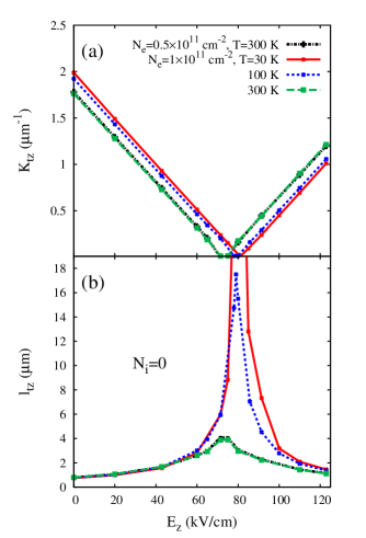
Figure 1: (Color online) $E_{z}$ dependence of (a) the spatial precession frequency and (b) the corresponding spin diffusion length at different temperatures and electron densities. The impurity density $N_{i}=0$ and the spin polarization is along the $z$-axis.

As shown in Fig. 1(a), $K_{tz}$ is approximately proportional to $|E_{z}-E_{z}^{c}|$, where the cancellation electric field $E_{z}^{c}$ is calculated from Eq. (2) ($E^{c}_{z}=82$ kV/cm at 30 K, $80$ kV/cm at 100 K, and $77$ kV/cm at 300 K). This originates from the weak momentum dependence of $\beta_{k}$ out of the strong cancellation regime, where $k^{2}\ll 4{\langle k_{z}^{2}\rangle-2\sqrt{3}\alpha eE_{z}^{c}/\gamma}$. In Fig 1(b), a peak is clearly seen in the $E_{z}$ dependence of the spin diffusion length. One finds that this peak locates just around $E_{z}^{c}$, which suggests that the peak should originate from the cancellation effect of the Dresselhaus and Rashba terms. Furthermore, it is revealed that the temperature and the electron density have marginal influence on the spin diffusion length for $E_{z}$ far away from $E^{c}_{z}$ as predicted by Eq. (14). However, when $E_{z}$ is around $E^{c}_{z}$, $\beta_{k}$ is strongly dependent on the moment and Eq. (14) fails for the inelastic scattering as we explained in Sec. II. In this case, one finds that, the spin diffusion length at the peak becomes shorter as the temperature increases. The underlying physics lies in the fact that, for higher temperature, the electrons disperse into a broader range in the ${\bf k}$ space, which means that fewer electrons are located in the regime with the in-plane Dresselhaus term significantly canceled by the Rashba term.Vurgaftman One also notices that the spin diffusion length for $N_{0}=0.5\times 10^{11}$ cm^-2 (with the Fermi temperature $T_{F}\approx 21$ K) is almost the same as that for $10^{11}$ cm^-2 ($T_{F}\approx 41$ K) at room temperature. This is because that the inhomogeneous broadening as well as the scattering strength (dominated by the electron-phonon scattering) is weakly dependent on the electron density in the non-degenerate regime at high temperature. When the electron gas enters into the degenerate regime, we find that the spin diffusion length can be tuned via the electron density. For example, the diffusion length changes from 17.5 $\mu$m to 15.2 $\mu$m as the density increases from $10^{11}$ to $4\times 10^{11}$ cm^-2 ($T_{F}\approx 166$ K) for $E_{z}=79$ kV/cm at 100 K.

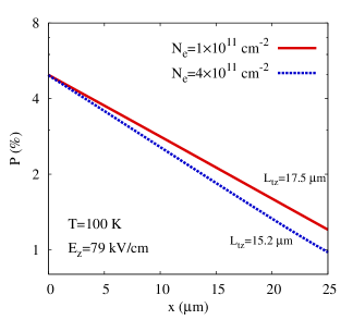
Figure 2: (Color online) The magnitude of the steady-state spin polarization as function of the position at 300 K with $N_{0}=10^{11}$ cm^-2 and $N_{s}=aN_{i}/N_{0}$.

To observe the role of the scattering strength further, we introduce the impurities into our GaAs QWs. The magnitude of the spin polarization with and without impurities are plotted as function of position in Fig. 2. In the absence of the perpendicular electric field, far away from the cancellation condition, the additional impurity scattering channel only slightly changes the spin diffusion length ($\sim 1$ %) which is consistent with Eq. (14). However, around $E^{c}_{z}$, the spin diffusion can be significantly influenced by the high doping density as shown in the figure, where $L_{tz}$ changes from 4.0 (3.0) to 3.3 (2.7) $\mu$m with $E_{z}=75$ (80) kV/cm by introducing the impurities.

We also investigate the anisotropy of the spin diffusion by taking the injection and detection polarizations along different directions. The position dependence of the magnitude of the spin polarization with $E_{z}=0$ and $79$ kV/cm are plotted in Fig. 3, where the notation $i$-$j$ means the injected spin polarization along $i$-direction and the detected one along $j$-direction. Since the signal in the $x$-$y$, $y$-$x$, $y$-$z$ and $z$-$y$ configurations are negligible as predicted by Eqs. (9)-(14), we only show the relevant components in the figure. For $E_{z}=79$ kV/cm, in the vicinity of the cancellation electric field, the spin polarizations for the $x$-$z$ and $z$-$x$ configurations also vanish due to the absence of the spatial spin precession. Interestingly, it is seen from Fig. 3 that the spin diffusion lengths for the $x$-$x$ and $z$-$z$ cases for $E_{z}=0$ kV/cm are equal

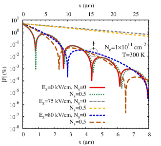
Figure 3: (Color online) The magnitude of the steady-state spin polarization as function of the position with different polarization directions in the absence of impurity. We take T=100 K and $N_{0}=10^{11}$ cm^-2. Here, $i$-$j$ represents the measured spin projection along $j$-axis while the injected spin polarization is along $i$-axis.

[$L_{tx}=L_{tz}=0.76$ $\mu$m and $L_{ty}=0.51$ $\mu$m, well consistent with the relation $l_{x}=l_{z}\approx 1.48l_{y}$ from Eqs. (9)-(14)], while the $x$-$x$ and $y$-$y$ cases share the same spin diffusion length ($L_{tx}=L_{ty}=9.3$ $\mu$m and $L_{tz}=17.8$ $\mu$m) for the electric field $E_{z}=79$ kV/cm. In the latter case without spatial spin precession, the drift-diffusion model performs well.Zhanggraphene Therefore, the spin diffusion length can be expressed by $L_{{\bf\hat{n}}}=\sqrt{D_{s}\tau_{s{\bf\hat{n}}}}$ with $\tau_{s{\bf\hat{n}}}\sim 1/\overline{(|{\mbox{\boldmath$\Omega$\unboldmath}}({\bf k})|^{2}-\Omega^{2}_{\bf\hat{n}})\tau_{p}}$ standing for the spin relaxation time. $D_{s}$ denotes the spin diffusion constant and $\tau_{p}$ represents the momentum relaxation time.wuReview ; opticalorientation According to Eq. (1), one has $\overline{|{\mbox{\boldmath$\Omega$\unboldmath}}({\bf k})|^{2}-\Omega^{2}_{x}}=\overline{|{\mbox{\boldmath$\Omega$\unboldmath}}({\bf k})|^{2}-\Omega^{2}_{y}}\approx 3.3\overline{|{\mbox{\boldmath$\Omega$\unboldmath}}({\bf k})|^{2}-\Omega^{2}_{z}}$, which lead to the relation $L_{x}=L_{y}\approx 0.55L_{z}$ by considering $D_{s}$ and $\tau_{p}$ free from the small spin polarization. This agrees well with the result from the KSBEs ($L_{tx}=L_{ty}\approx 0.52L_{tz}$).

Finally, we should point out that the correction of the envelope function due to the perpendicular electric field is neglected, even though it can modify the spin orbit coupling via the quantity $\langle k_{z}^{2}\rangle$ and the scattering strength via the form factor in the scattering term.Zhou ; weng This is because: (i) the modification of $\langle k_{z}^{2}\rangle$ due to electric field is quite small (within 3 %); (ii) the spin diffusion is insensitive to the scattering strength as discussed above. Direct calculation shows that only slight modification of the diffusion length is introduced by the electric field, for example, around 3 % at 100 K with $E_{z}$=79 kV/cm.

IV CONCLUSION

In conclusion, we have investigated the spin diffusion in $n$-type (111) GaAs QWs by solving the microscopic KSBEs. In the perpendicular electric dependence of the spin diffusion length, a peak due to the cancellation between the in-plane Dresselhaus spin-orbit coupling and the Rashba term is predicted. We find that, for the perpendicular electric field away from the strongest cancellation value, the spin diffusion length is insensitive to the electron density, temperature, and doping density. However, in the vicinity of the cancellation electric field, the spin diffusion length shows strong dependence on the temperature and doping density. For high electron density, the electron gas is degenerate, and the spin diffusion length is found to be also affected by the electron density. Finally, we uncover the anisotropic spin diffusion with respect to the spin polarization direction.

- (1) Optical Orientation, edited by F. Meier and B. P. Zakharchenya (North-Holland, Amsterdam, 1984).
- (2) S. A. Wolf, D. D. Awschalom, R. A. Buhrman, J. M. Daughton, S. von Molnár, M. L. Roukes, A. Y. Chtchelkanova, and D. M. Treger, Science 294, 1488 (2001).
- (3) Semiconductor Spintronics and Quantum Computation, edited by D. D. Awschalom, D. Loss, and N. Samarth (Sprinter, Berlin, 2002).
- (4) I. uti, J. Fabian, and S. Das Sarma, Rev. Mod. Phys. 76, 323 (2004); J. Fabian, A. Matos-Abiague, C. Ertler, P. Stano, and I. uti, Acta Phys. Slov. 57, 565 (2007); Spin Physics in Semiconductors, edited by M. I. D’yakonov (Springer, Berlin, 2008); and references therein.
- (5) M. W. Wu, J. H. Jiang, and M. Q. Weng, Phys. Rep. 493, 61 (2010); and references therein.
- (6) Z. G. Chen, S. G. Carter, R. Bratschitsch, and S. T. Cundiff, Physica E 42, 1803 (2010).
- (7) T. Korn, Phys. Rep. 494, 415 (2010).
- (8) M. M. Glazov, E. Ya. Sherman, and V. K. Dugaev, Physica E 42, 2157 (2010).
- (9) N. Tombros, C. Jozsa, M. Popinciuc, H. T. Jonkman, and B. J. van Wees, Nature (London) 448, 571 (2007).
- (10) S. Datta and B. Das, Appl. Phys. Lett. 56, 665 (1990).
- (11) J. Wunderlich, B. G. Park, A. C. Irvine, L. P. Zârbo, E. Rozkotová, P. Nemec, V. Novák, J. Sinova, and T. Jungwirth, Science 330, 1801 (2010).
- (12) H. C. Koo, J. H. Kwon, J. Eom, J. Chang, S. H. Han, and M. Johnson, Science 325, 1515 (2009).
- (13) M. I. D’yakonov and V. I. Perel’, Zh. ksp. Teor. Fiz. 60, 1954 (1971) [Sov. Phys. JETP 33, 1053 (1971)].
- (14) M. W. Wu and C. Z. Ning, Eur. Phys. J. B 18, 373 (2000); M. W. Wu, J. Phys. Soc. Jpn. 70, 2195 (2001).
- (15) J. H. Jiang, Y. Zhou, T. Korn, C. Schüller, and M. W. Wu, Phys. Rev. B 79, 155201 (2009).
- (16) J. H. Jiang and M. W. Wu, Phys. Rev. B 79, 125206 (2009).
- (17) G. Dresselhaus, Phys. Rev. 100, 580 (1955).
- (18) Y. A. Bychkov and E. I. Rashba, J. Phys. C 17, 6039 (1984); Pis’ma Zh. ksp. Teor. Fiz. 39, 66 (1984) [JETP Lett. 39, 78 (1984)].
- (19) N. S. Averkiev and L. E. Golub, Phys. Rev. B 60, 15582 (1999).
- (20) J. Schliemann, J. C. Egues, and D. Loss, Phys. Rev. Lett. 90, 146801 (2003).
- (21) J. L. Cheng, M. W. Wu, and I. C. da Cunha Lima, Phys. Rev. B 75, 205328 (2007).
- (22) L. P. Zârbo, J. Sinova, I. Knezevic, J. Wunderlich, and T. Jungwirth, Phys. Rev. B 82, 205320 (2010).
- (23) X. Cartoixà, D. Z.-Y. Ting, and Y.-C. Chang, Phys. Rev. B 71, 045313 (2005).
- (24) I. Vurgaftman and J. R. Meyer, J. Appl. Phys. 97, 053707 (2005).
- (25) B. Y. Sun, P. Zhang, and M. W. Wu, J. Appl. Phys. 108, 093709 (2010).
- (26) J. L. Cheng and M. W. Wu, J. Appl. Phys. 101, 073702 (2007).
- (27) P. Zhang and M. W. Wu, Phys. Rev. B 79, 075303 (2009).
- (28) P. Zhang and M. W. Wu, arXiv:1012.0973v1.
- (29) H. Haug and A. P. Jauho, Quantum Kinetics in Transport and Optics of Semiconductors (Springer, Berlin, 1996).
- (30) J. Zhou, J. L. Cheng, and M. W. Wu, Phys. Rev. B 75, 045305 (2007).
- (31) M. Q. Weng, M. W. Wu, and L. Jiang, Phys. Rev. B 69, 245320 (2004).
- (32) T. Hassenkam, S. Pedersen, K. Baklanov, A. Kristensen, C. B. Sorensen, P. E. Lindelof, F. G. Pikus, and G. E. Pikus, Phys. Rev. B 55, 9298 (1997).
- (33) The asymptotic standard errors are less than 0.1% in the worst case.