Scientific Inquiry 7, No. 1, June 30, pp. 25 - 50 (2006).                   IIGSS Academic Publisher

Reasons for nuclear forces in light of
the constitution of the real space

Volodymyr Krasnoholovets

22 April 2005

Abstract

The concept of microstructure of the real space, considered as a mathematical lattice of cells (the tessellattice), and notions of canonical particles and fields, which are generated by the space, are analyzed. Submicroscopic mechanics based on this concept is discussed and employed for in-depth study of the nucleon-nucleon interaction. It is argued that a deformation coat is developed in the real space around the nucleon (as is the case with any other canonical particle such as electron, muon, etc.) and that they are the deformation coats that are responsible for the appearance of nuclear forces. One more source of nuclear forces is associated with inerton clouds, excitations of the space tessellattice (the excitations are a substructure of nucleons’ matter waves), which accompany moving nucleons as in the case of any other canonical particles. Two nuclear systems are under consideration: the deuteron and a weight nucleus. It is shown that a weight nucleus is a cluster of interacting protons and neutrons. The condition of the cluster stability is obtained in the framework of the statistical mechanical approach. On the whole, the paper proposes a radically new approach to a very old unsolved problem, the origin of the nuclear forces, allowing the understanding mechanism(s) occurring at low energy nuclear transmutations.

Key words: inertons, nucleons, nuclear forces, quantum mechanics, space structure, tessellattice

PACS: 21.30.-x nuclear forces;  21.80.+a hypernuclei;  21.60.Gx cluster models;   24.80.+y nuclear tests of fundamental interactions and symmetries;  24.60.-k statistical theory and fluctuations;  11.90.+t other topics in general theory of fields and particles

1. Introduction and preliminaries

1.1. Conventional views

Although nuclear physics is a well-developed branch of modern physical science, avenues for the resolution of the problem of the origin of nuclear forces are still beyond understanding. At present the model approach to deriving nuclear forces from the quark-quark interaction prevails among researchers. Nevertheless, such an approach is open to question, especially owing to the confinement problem, which is the most difficult one for quantum chromodynamics (QCD).

It is a matter of fact that the understanding how QCD works remains one of the great puzzles of many-body physics. Indeed, the degrees of freedom observed in low energy phenomenology are totally different from those appearing in the QCD Lagrangian. In the case of many-nucleon systems, the question of the origin of the nuclear energy scale is immediately arouse: the typical energy scale of QCD is on the order of 1 GeV, though the nuclear binding energy per particle is very small, on the order of 10 MeV. Is there some deeper insight from which this scale naturally arises? Or the reason should one searches in complicated details of near cancellations of strongly attractive and repulsive terms in the nuclear interaction?

This large separation between the hadronic energy scale and the nuclear binding scale has led to an alternative approach, especially at the description of the physics of small A nuclei. Namely, effective field theory techniques, which arise from chiral symmetry, allow quantitative calculations of energy parameters of such nuclei. In particular, these methods have been employed to account for the physics of pions in the context of chiral perturbation theory. Currently efforts are made to combine these effective field theories with the low energy constants from QCD, which then might be considered as first principles calculations. A further fundamental progress is expected from the lattice field theory and the use of super computers.

Nevertheless, recent high precision measurements (Gilman and Gross [1]) of the deuteron electromagnetic structure functions (A, B and $T_{20}$) extracted from high-energy elastic ed scattering, and the cross sections and asymmetries extracted from high-energy photodisintegration $\gamma+d\rightarrow n+p$, have been reviewed and compared with the theory. The theoretical consideration included nonrelativistic and relativistic models using the traditional meson and baryon degrees of freedom, effective field theories, and models based on the underlying quark and gluon degrees of freedom of QCD, including nonperturbative quark cluster models and perturbative QCD. The conclusion has been drawn that analyzes of the elastic ed scattering experiment and the photodisintegration experiment require very different theoretical approaches.

In other words, the rigorous results of work [1] demonstrate that QCD and the meson theory seem disagree. Hence the origin of nuclear forces in a unperturbed nucleus is still unclear.

1.2. Hadronic mechanics

Although QCD and quantum field theories are rather considered as independent disciplines, they, however, are strongly based on nonrelativistic and relativistic quantum mechanics. Santilli proposed (see, e.g. Ref. [2,3]) the broadening foundations of quantum mechanics known under the title of hadronic mechanics. This mechanics has been developing now by numerous researchers both theoreticians and experimentalists. In particular, hadronic mechanics has successfully been applied for the study of stimulated nuclear transmutations in the range of low and intermediate energies [2].

Santilli has shown [2] how conventional quantum mechanics is insufficient to solve its most fundamental problem: the physical origin of the strong interaction of nuclear constituents (a number of potentials used does not give any explanation whatever of the origin of attraction between nucleons); the theoretical prediction of quantum mechanics for the correct representation of the deuteron in its ground state misses 2.3% of the experimental value. There are also other strong insufficiencies of quantum mechanics for the representation of nuclear data [2].

Regarding a possibility of deriving nuclear forces from the quark-quark interaction, Santilli [2] reasonably remarks that quarks can only be defined in a mathematical unitary space that has no direct connection to an actual physical reality. Then he continues: “It is known by experts that, because of the impossibility of being defined in our space-time, quarks cannot have any scientifically meaningful gravitation, and their “masses” are pure mathematical parameters in the mathematical space of SU(3) with no known connection to our space-time.” Indeed, quarks cannot be defined through special relativity and its fundamental Poincar${\rm\acute{e}}$ symmetry. Therefore, this means that mass cannot be introduced as the second order Casimir invariant, however, this is only the necessity for mass to exist in our space-time.

In other words, the basic challenge of deducing the gravitational interaction from quarks seems completely unfeasible.

Taking into account the mentioned fundamental difficulties, Santilli, developing hadronic mechanics, started from the hypothesis that in a system of strongly interacting particles the total Hamiltonian cannot be subdivided to kinetic and potential parts. Hadronic mechanics is constructed via a nonunitary transform of orthodox quantum mechanics, namely, the unitary character appears only at a distance larger than the radius of nuclear forces $r_{\rm n.{\kern 1.0pt}f.}\approx 10^{-15}$ m:

$$U\times U^{\dagger}={\hat{I}}\left\{\begin{array}[]{ll}\neq I&\textrm{for}\quad r\ll r_{\rm n.{\kern 1.0pt}f},\\ =I&\textrm{for}\quad r\gg r_{\rm n.{\kern 1.0pt}f.}.\\ \end{array}\right.$$

Then a simple yet in fact effective, realization of this assumption for the relativistic treatment of a system of two nucleons, i.e. deuteron, is Animalu-Santilli isounit [2]

$${\hat{I}}_{12}=\prod\limits_{k}{\rm Diag}\left(n^{2}_{1{\kern 1.0pt}k},n^{2}_{2{\kern 1.0pt}k},n^{2}_{3{\kern 1.0pt}k},n^{2}_{4{\kern 1.0pt}k}\right)\times\exp\left(N\int d{\kern 1.0pt}v{\kern 2.0pt}{\hat{\psi}}^{{\dagger}}_{\uparrow k}({\bf{r}})\times{\hat{\psi}}_{\downarrow{\kern 0.5pt}k}({\bf{r}})\right)$$

where $k=1,{\kern 1.0pt}2$. The functions $n^{2}_{ik}$ represent the shape of the nucleon and characterizes semiaxes of spheroidal ellipsoids normalized to the values for the perfect shape and to the volume preserving simple conditions.

Such a transform allows the introduction of a modernized Lie product, Pauli matrices, Dirac equation, etc. So, the conventional Hamiltonian of relativistic quantum mechanics and the appropriate spinors are transformed to a new Santilli’s isomathematical presentaions. The mathematics developed enabled the calculation of basic parameters of nuclear systems, which exactly agreed the experimental data [2].

Unlike conventional quantum mechanics that operate with point particles and their appropriate wave packets, or wave functions, hadronic mechanics deals with the extended particles that feature peculiar shapes in our space-time.

Hadronic mechanics indeed yields remarkable predictions both in chemical and nuclear physics. In particular, it has predicted new stable chemical species such as hydrogen and etc., which have been verified experimentally, and which are specified by the stronger binding energy of electrons with atoms (around 2 times larger than in case of conventional species). A similar hypothesis has been offered for the structure of the neutron: the neutron has been treated as a strongly coupled proton-electron pair. This enabled one to associate the nuclear forces with the pure Coulomb interaction between protons and neutrons. Thus in hadronic mechanics the origin of nuclear forces is complete plain: this is the usual Coulomb interaction between nucleons.

1.3. Submicroscopic consideration

QCD, effective quantum theories and hadronic mechanics widely employ notions and means of orthodox quantum mechanics, first of all Schrödinger’s wave $\psi$-function and Dirac’s spinor formalisms, which themselves are exposed to significant conceptual difficulties [4].

Nonlocality, which the wave $\psi$-function introduced, and action at-a-distance forces are the most challenging questions of orthodox quantum mechanics [4]. In fact, in quantum mechanics all potentials are treated as static and long-distance: a parabolic potential in the harmonic oscillator problem, the Coulomb potential in the hydrogen atom problem, etc. (see also Arunasalam [5]).

So, all modern quantum theories including quantum mechanics, QCD, hadronic mechanics and etc. imply long-range action. Therefore, in this respect they do not differ from the phenomenological Newton’s gravitational law, which indeed establishes the link $G{\kern 1.0pt}M_{1}M_{2}/r$ between two distant objects, but does not account for the mechanism that realizes the interaction. General relativity also does not account for the origin of Newton’s potential, but simply employs it as a starting point complicating the theory.

Moreover, no one of quantum theories available does pay any attention to the background of systems studied, i.e. the structure and peculiarities of the real physical space. The theories are developed in abstract spaces: energy, momentum, phase, Hilbert and so on. Instead of the background space they use such complete undetermined notions as a “physical vacuum” or/and an “aether” providing them with every possible and imaginary properties. It seems the aforementioned Santilli’s quotation regarding quarks as objects that are not determined in the space-time is the apt turn of phrase, which emphasizes the validity of our criticism.

Having overcome difficulties of quantum physics caused by the deficiency of knowledge about the background, Bounias and the author [6-9] have recently undertaken an in-depth study of space as it is. Starting from topology, set theory and fractal geometry we have revised the principal mathematical notions, by which time the mathematical and physical literature has presented.

We have based our consideration [6-9] on the assumption that the real space, i.e. a 3D space or a 4D space-time, is not a dim vacuum but a quantum substrate that shares discrete and continual properties. Similarly to condensed matter physics in which the availability of a regular/irregular atom lattice plays the fundamental role, we have introduced a special mathematical lattice of topological balls, which characterizes the real space in detail. This space generates matter (particles) and provides for the creation of physics laws. In particular, the interaction of a particle with the surrounding space, cells of the mathematical lattice called the “tessellattice”, has to produce short-range action, i.e. excitations of the tessellattice, which are capable of carrying the interaction for long distances from the particle, as in the case of excitations of the crystal lattice of a solid.

A particle appears as a local deformation of the tessellattice. The deformed cell being stable represents an actual core of any canonical particle.

It is assumed [10] that the size of a superparticle, the building block of the tessellattice, is on the order of $10^{-30}$ m. In fact, it is known that on this scale three of four physical interactions (electromagnetic, weak and strong, except for the gravitational interaction) should come together. Besides, in particle physics researchers use the notion of an abstract superparticle whose different states are electron, positron, muon, quarks, etc.

A cell deformation of the tessellattice means the induction of mass in the appropriate cell and the value of mass is directly proportional to the degree of the cell deformation. Such deformation can only be the fractal deformation [7,8]. Besides, the class of leptons (electron, muon and $\tau$-lepton) is characterized by the fractal reduction of the initial volume of a cell, though the class of quarks features the fractal expansion of the initial volume of a cell [8,9].

The electric charge is associated with a quantum of fractality that is complete located in one cell [8,9]. The charge state is located on the surface of the particled cell. A positive charged particle has naturally been determined as an object whose surface covered by protuberances, then a negative charged particle is specified by the surface covered by cavities [8,11]. A detailed theory of the charge and the submicroscopic interpretation of the Maxwell equations have been developed in paper [11].

The theory of the real space allows the construction of a mechanics of particles, which incorporates the interaction of a moving particle with the tessellattice essentially representing the degenerate, or non-manifest, state of the space. In other words, this is a dynamics of the mathematical lattice, the tessellattice, which being developed will complete substitute all modern theories and their attempts aimed at the construction of a unified theory of the nature.

In the present work we briefly describe submicroscopic quantum mechanics developed in the real space, which has been constructed by the author [12-16]. It should be emphasized that the theory has successfully been verified experimentally [17-19] and agree well with many data. Then the results obtained in the framework of submicroscopic approach are applied to the consideration of nuclei. That is, we will study peculiarities of the nucleon structure, which generate nuclear forces, and disclose the inner reasons for these forces. After that we will investigate actual trajectories of nucleons in the deuteron, i.e. trajectories of the deuteron’s nucleons in the real space. Furthermore, we will analyze the origins of major potentials, which are present in weight nuclei and which show that a nucleus should be treated as a cluster of nucleons.

2. Dynamics of tessellattice

We have shown [6-9] that the universe indeed can be constructed of nothing, or in other words, the universe allows the description in the form of a mathematical lattice of empty sets, i.e. degenerate cells that can be called superparticles. Obviously, a dynamics of the mathematical lattice, called the tessellattice [6-9], should include all possible kinds of transformations and movements allowable by the combinations of mathematical rules in the structure of packed cells taking into account possible cells’ shapes and kinds of symmetries, the inversion of cell deformation (e.g., the transition quark - lepton), the exchange of fractal deformations, and the real motion of deformed cells, i.e. particles, in the tessellattice. The theory of dynamics of the tessellattice is still in the rudimentary state and its further development will need the tremendous work of numerous researchers.

At the same time, the motion of a particle in the tessellattice should be related to pure mechanics, but what kind of a mechanics? The problem has been studied by the author in a series of works [4,10-19]. The research has shown that the mechanics of particles in the tessellattice (i.e. in the real space) constitutes submicroscopic deterministic quantum mechanics, because it is easily reduced to the formalism of conventional quantum mechanics: Schrödinger’s [12,13] and Dirac’s [14], which is developed in abstract phase or Hilbert spaces.

We recall that quantum mechanics, as such, being based on indeterminism is constructed in the phase space and establishes probabilistic links between measurable characteristics of the system studied. The most essential characteristics, or parameters, of particles are their energy, momentum, moment of momentum, and position. Submicroscopic deterministic quantum mechanics, which is called submicroscopic mechanics below, makes broader the framework of orthodox quantum mechanics. The deterministic approach has been constructed in the real space in which the particle’s parameters mentioned above are determined. Thus submicroscopic mechanics being developed in the real space allows causal links between the given particle parameters.

In submicroscopic mechanics, the creation of a canonical particle is treated as the appearance of a local deformation in the tessellattice, i.e. a stable change in the volume of a superparticle is associated with the formation of a massive particle. The mass is determined as the ratio between the initial volume of a superparticle in the degenerate state of the tessellattice and the volume of the same superparticle in the deformed state, $M_{{\kern 0.4pt}0}\propto{\kern 1.0pt}{\kern 1.0pt}{\kern 1.0pt}{\kern 1.0pt}{\kern 1.0pt}{\mathcal{V}}^{\left({\rm sup}\right)}/{\kern 1.0pt}{\kern 1.0pt}{\mathcal{V}}^{\left({\rm part}\right)}$. A quasi-particle, or elementary excitation of the space tessellattice, is also associated with the appearance of a local deformation that is small and unstable in comparison with a particle; the mass of an excitation of the tessellattice $m_{{\kern 1.0pt}0}\propto{\kern 1.0pt}{\kern 1.0pt}{\kern 1.0pt}{\kern 1.0pt}{\kern 1.0pt}{\mathcal{V}}^{\left({\rm sup}\right)}/{\kern 1.0pt}{\kern 1.0pt}{\mathcal{V}}^{\left({\rm excit}\right)}$. Therefore, $M_{{\kern 0.4pt}0}\gg m_{{\kern 0.3pt}0}$.

Note that in the case of mechanics, there is no need to take into account peculiarities of the volume decrease of a cell, which results in the induction of mass in the corresponding cell. Although the pure volume decrease is not sufficient for providing a cell with mass; only the fractal-related decrease of the volume of the cell causes an actual deformation that is associated with mass [7,9].

In solid state physics, the occurrence of a foreign particle in the crystal lattice automatically induces a range of a deformation in the crystal lattice, i.e. the so-called deformation coat, which covers from several lattice constants to several tens of the lattice constants. By analogy, we should construct a deformation coat around a canonical particle in the tessellattice, which plays the role of a screen that separates the particle from the degenerate space. Indeed a particled cell should be characterized by a strong local deformation. Hence the tessellattice should responses to this deformation in such a way that all cells in a range $R$ around the particled cell become deformed down to the boundary where edge cells are bounded by a rupture of the remaining fractality. We equal the size $R$ of the deformation coat to the Compton wavelength $\lambda_{{\kern 1.0pt}\rm Com}=h/M_{0}{\kern 1.0pt}c$ of the particle in question [14]. Hence the radius of the deformation coat coincides with the value of $\lambda_{{\kern 1.0pt}\rm Com}$. Since cells, or superparticles, inside the coat are deformed, they possess mass as well as the particle that is found in the center of the formation.

When a particle starts to move with a velocity $v$, it pushes its way through coming fluctuating superparticles and thus the particle collides with superparticles. Owing to the interaction with coming superparticles the particle has to emit elementary excitations. As the excitations represent inert properties of the particle, they were called “inertons” [12-14]; inertons are generated due to the resistance of the space that the moving particle experiences (see also Ref. [7]). The moving particle also pulls its deformation coat, but superparticles in the coat remain motionless. The superparticles’ massive state travels by a relay mechanism, i.e. the particle adjusts surrounding superparticles to the deformation coat state; it is suggested that this state is adjusted with a speed no less than the speed of light c.

The particle emits inertons along a section $\lambda/2$ of its path and hence it loses the velocity, $v\to 0$; on the next section $\lambda/2$ the elastic tessellattice sends inertons backward to the particle and the particle velocity is restored to the value $v$ and so on. The section $\lambda$ is the equivalent of the de Broglie wavelength of the particle. In such a manner inertons make up a substructure of the matter waves and therefore they should be considered as carriers of the quantum mechanical force, or quantum mechanical potential, generated by the particle in the ambient space. The velocity of inertons cannot be lesser than the speed of light c. Thus inertons allow us to completely remove long-range action from quantum mechanics.

Inertons transmitting the energy and the momentum also carry fragments of local deformation of the tessellattice, i.e. they atomize the particle’s inert mass in the surrounding of the particle. This means that the mentioned quantum mechanical potential (or the deformation of the space) should be identified with the gravitational potential of the particle. This problem has been studied in detail in papers [21,16] where the process of inerton emission and the reentry of inertons into the particle have also been investigated. The transition to the formalism of orthodox quantum mechanics takes place by relationships

$$E=h{\kern 1.0pt}{\kern 1.0pt}\nu,\quad\quad\lambda=\frac{{h}}{{p}},$$ (1)

which are derived in the frame of the submicroscopic consideration.

Relationships (1) were first written down for a particle by Louis de Broglie in 1924 (see, e.g. Ref. [20]) and then were derived by the author [12,13] in the framework of the submicroscopic approach briefly stated herein. The availability of relationships (1) enables [20] a simple derivation of the Schrödinger wave equation.

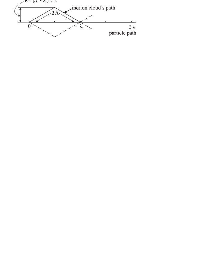
Figure 1: Schematic representation of the section $\lambda$ along the particle path and the effective path length $2\Lambda$ of the particle’s inerton cloud.

In the submicroscopic approach the parameter E is equal to the total kinetic energy of the particle $\tfrac{{1}}{{2}}M_{0}v^{2}/\sqrt{1-v^{2}/c^{2}};\quad\nu$ denotes the frequency of oscillations of the particle along its path, namely, the frequency of the oscillation of the particle’s velocity due to the periodic emission and reabsorption of inertons, $v\to 0\to v\to 0\to...$ (besides, $\nu$ is connected with the period of collisions $T$ of the particle with its inerton cloud, $\nu=1/2T$); the de Broglie wavelength $\lambda$ represents here the spatial period, or amplitude, of oscillations of the particle along its path; $p=M_{\kern 1.0pt0}v/\sqrt{1-v^{2}/c^{2}}$ is the total momentum of the particle.

The mentioned parameter T also enables other presentations: $T=v\lambda$ and $T=c\Lambda$ where $\Lambda$ is the free path length of the cloud of inertons, which the cloud passes between two sequential collisions with the particle ($\Lambda$ can also be called the amplitude of the inerton cloud). Similarly, $\lambda$ can be called the free path length of the particle. Such a presentation makes it possible to consider the particle’s behavior in terms of kinetic theory. The particle’s path and the particle’s parameters $\lambda$ and $\Lambda$ are sketched in Figure 1. As follows from Figure 1, the range covered by the inerton cloud around the particle can be estimated by a radius $R=\sqrt{\left({\Lambda/2}\right)^{2}-\left({\lambda/2}\right)^{2}}$, i.e. $R\sim\Lambda$.

So, the availability of the inerton cloud enclosing a canonical particle endows the abstract (probabilistic) wave $\psi$-function with an actual physical sense: The $\psi$-function covers the range of the space disturbed by the moving particle, $R\sim\Lambda$, and sets up links between the parameters of the particle and those of the particle’s inerton cloud. In other words, the $\psi$-wave function describes the inerton field of the particle, which spreads out of the particle up to the range $\sim\Lambda$.

Equating relations $T=v\lambda$ and $T=c\Lambda$, we get the relationship

$$\Lambda=\lambda{\kern 1.0pt}{\kern 1.0pt}\frac{{c}}{{v}}{\kern 4.0pt}$$ (2)

that relates the particle parameters $\lambda$ and $v$ to corresponding parameters of the particle inerton cloud, $\Lambda$ and $c$. Relationship (2) can be rewritten by using the Compton wavelength $\lambda_{{\kern 1.0pt}{\kern 1.0pt}\rm Com}$ of the particle,

$$\Lambda=\lambda_{{\kern 1.0pt}{\kern 1.0pt}\rm Com}{\kern 2.0pt}{\kern 1.0pt}\frac{{c^{2}}}{{v^{2}}}{\kern 4.0pt}.$$ (3)

We see from expression (3) that when the particle velocity $v$ tends to $c$, the inerton cloud becomes practically closed in a range embraced by the Compton wavelength, or in other words, the deformation coat (or the space crystallite) that is developed around the particle in the space tessellattice.

The submicroscopic quantum theory stated above could be usefully employed in the studies of those quantum systems to which conventional quantum mechanics is also applied. Perhaps the main value of the submicroscopic approach is its short-range action, which so far has been overlooked in the other concepts. Besides, submicroscopic mechanics could solve such difficult theoretical problems as disagreement on the Schrödinger equation and Lorentz invariance [13], the interpretation of the spin [14,8], the nature of the phase transition that occurs in the quantum system under consideration when we pass from the description based on the Schrödinger formalism to that resting on the Dirac one [14], the origin of gravity [16,21], the nature of the photon [22,11] and so on. Moreover, the theory has predicted the existence of a new physical field – the inerton field – that then has successfully been fixed experimentally [17] (see also Refs. [18,19]).

All these results allow us to anticipate that the submicroscopic approach should also be useful when considering the intricate challenge associated with the nature of nuclear forces, the more so, as experimentalists who investigate low energy nuclear reactions claim that they fix a new “strange” radiation at the transmutation of nuclei [23,24]. Clearly, that “strange” radiation was nothing else as inertons, which radiated from the appropriate inerton clouds of nucleons when the latter rearranged in nuclei.

3. Deformation coat of the nucleon

Since superparticles in the deformation coat surrounding a particle possesses masses, they should fall within collective vibrations by analogy with massive entities (atoms, molecules) in the crystal lattice. This analogy has also allowed us to call the deformation coat the space crystallite and then to investigate its vibratory mode [14]. In the crystallite, vibrations of all superparticles co-operate and the total energy of superparticles, which is equal to the total energy of the particle, $M_{{\kern 1.0pt}0}{\kern 1.0pt}c^{2}$, is quantized,

$$\hbar{\kern 1.0pt}{\kern 1.0pt}\omega_{k_{0}}=M_{{\kern 1.0pt}0}{\kern 1.0pt}c^{2}$$ (4)

where $k_{{\kern 1.0pt}0}=2\pi/\lambda_{{\kern 1.0pt}\rm Com}$ is the wave number and $\omega_{k_{{\kern 1.0pt}0}}=ck_{{\kern 1.0pt}0}$ is the cyclic frequency of an oscillator in the $k$-space (the quantity $\lambda_{{\kern 1.0pt}\rm Com}$ is the amplitude of the oscillator, which is given by the crystallite size, i.e. the Compton wavelength). For the moving particle expression (4) is transformed to

$$\hbar{\kern 1.0pt}{\kern 1.0pt}\omega_{k_{v}}=M{\kern 1.0pt}c^{2}$$ (5)

where $M=M_{{\kern 1.0pt}0}/\sqrt{1-v^{2}/c^{2}}$ and $k_{{\kern 1.0pt}v}=2\pi/\left({\lambda_{{\kern 1.0pt}\rm Com}/\sqrt{1-v^{2}/c^{2}}}\right)$. The crystallite travels together with the particle, namely, coming superparticles adjust to the massive state in the range covered by the crystallite size $\lambda_{{\kern 1.0pt}\rm Com}/\sqrt{1-v^{2}/c^{2}}$ by a relay mechanism with a speed no less than the speed of light $c$.

Figure 2 depicts the deformation coat, or crystallite, that is progressing around the canonical particle in the degenerate tessellattice. Figure 2 rather sketches the spatial pattern of a lepton (electron, positron, muon, etc.).

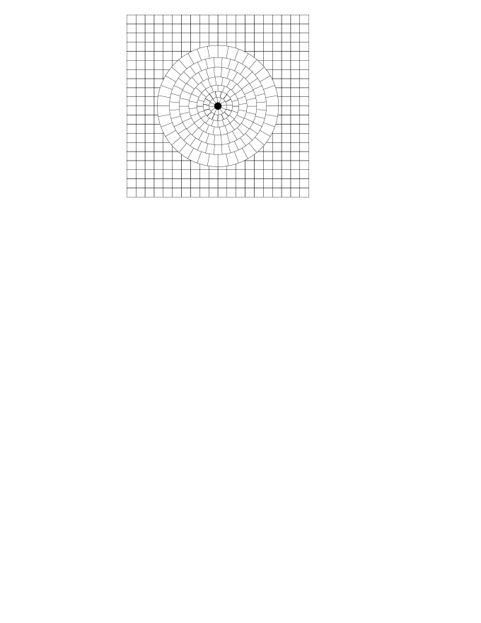
Figure 2: Canonical particle surrounded by its deformation coat, or space crystallite, in the space tessellattice.

In the case of a quark we should anticipate a similar picture, though the quark itself and superparticles in its deformation coat should be characterized by a deformation that is inverse in comparison with that that specifies leptons and superparticles in the lepton’s coat. This is the only feature that distinguishes a family of quarks from that of leptons and only this feature can account for the non-stability of isolated quarks. The only way for quarks to survive is their integration into groups of a smaller total size, hadrons, which have to lower the degree of the inverse deformation of space associated with the quark and thus should stabilize them. Here we will not analyze peculiarities of the spatial pattern of quarks in a hadron and the motion of quarks in it (though the motion should not in principle be disobedient to the rules of submicroscopic mechanics stated above). We shall restrict our consideration to the fact that the hadron features first quarks’ generalized deformation coat and then an outer, or usual deformation coat shown in Figure 3 in which superparticles of the space tessellattice have a smaller size than that in the degenerate state.

For the nucleon we may ascribe the radius $R_{{\kern 1.0pt}\rm c}\simeq 0.4\times 10^{-15}$ m to the quark’s generalized deformation coat, because on this size, as is known (see, e.g. Ref. [25]), nuclear forces of attraction are converted into forces of repulsion. The masses of nucleons, $M_{0{\kern 1.0pt}\rm neutron}\cong M_{0{\kern 1.0pt}\rm proton}=M_{{\kern 1.0pt}0}=1.67\times 10^{-27}$ kg and therefore the nucleon’s Compton wavelength $\lambda_{{\kern 1.0pt}{\kern 1.0pt}\rm Com}=h/M_{0}{\kern 1.0pt}c=1.32\times 10^{-15}$ m. This magnitude should be identified with an actual radius of the (outer) deformation coat of the nucleon. Figure 3 depicts the nucleon in the real space: there is the main body (the hadron core) with the radius $R_{\rm c}\simeq 0.4\times 10^{-15}$ m in the center part, which includes three quarks, and the deformation coat (crystallite) surrounding the core with the radius $\lambda_{{\kern 1.0pt}{\kern 1.0pt}\rm Com}=1.32\times 10^{-15}$ m.

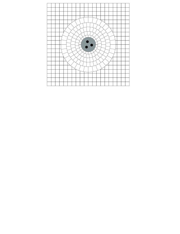
Figure 3: Degenerate space and the nucleon, which consists of the main body, or core (shaded) and the deformation coat that surrounds the core.

Since the size of a nucleus $R\simeq R_{{\kern 1.0pt}0}{\kern 1.0pt}A^{1/3}$ where $R_{{\kern 1.0pt}0}=\left({1.2\,\,\,{\rm to}\,\,\,1.3}\right)\times 10^{-15}$ m and $A$ is the number of nucleons, we may identify the parameter $R_{{\kern 1.0pt}0}$ with the said Compton wavelength $\lambda_{{\kern 1.0pt}{\kern 1.0pt}\rm Com}$ and therefore $R_{{\kern 1.0pt}0}$ becomes the radius of the deformation coat of the nucleon. Beyond the coat superparticles are found in the degenerate state where they do not possess any mass.

3.1. Behavior of the deformation coat in the phase space

The value of the potential energy accumulated in the deformation coat of a nucleon ($M_{0{\kern 1.0pt}\rm n}{\kern 1.0pt}c^{2}$ for neutron and $M_{0{\kern 1.0pt}\rm p}{\kern 1.0pt}c^{2}$ for proton) stores up in the vibrating mode of the coat, which shows expression (5) that has been derived at the consideration in the energy space (see Appendix in Ref. [14]). Vibrations of atoms in the crystal lattice simplify periodical oscillations of atoms around their equilibrium positions. In the case of the deformation coat the vibratory process can occur according to a similar scenario. Besides, owing to the spherical form of the crystallite we may reduce the problem to the well-known task of mathematical physics on small vibrations of a gas contained in a sphere (see, e.g. Ref. [26]).

The velocities potential $u$ of the gas fulfills the wave equation

$$\frac{{\partial^{{\kern 1.0pt}2}u}}{{\partial{\kern 1.0pt}r^{2}}}+\frac{{2}}{{r}}\frac{{\partial{\kern 1.0pt}{\kern 1.0pt}u}}{{\partial{\kern 1.0pt}r}}=\frac{{1}}{{c^{2}}}\frac{{\partial{\kern 1.0pt}{\kern 1.0pt}u^{2}}}{{\partial{\kern 1.0pt}t^{2}}};$$ (6)

here $u$ for radial vibrations is a function of $r{\kern 1.0pt}$ and $t$ alone where $r{\kern 1.0pt}$ is the distance from a vibrating particle of the gas to the center of the sphere and $t$ is the time. Equation (6) is solved by substitution

$$u(r,{\kern 2.0pt}t)=w\left({r}\right){\kern 1.0pt}\theta\left({t}\right).$$ (7)

The surface of the sphere is treated as a hard envelope and therefore the normal component of the velocity is equal to zero, which leads to the boundary condition

$$\left.{\frac{{\partial{\kern 1.0pt}{\kern 1.0pt}w\left({r}\right)}}{{\partial{\kern 1.0pt}{\kern 1.0pt}r}}}\right|_{\,\,r=R_{{\kern 1.0pt}0}}\,=0$$ (8)

where $R_{{\kern 1.0pt}0}$ is the radius of the spherical envelope (the radius of the deformation coat). The solution for $w\left({r}\right)$ is

$$w\left({r}\right)=C{\kern 1.0pt}{\kern 1.0pt}{\kern 1.0pt}\frac{{\sin\left({\eta{\kern 1.0pt}{\kern 1.0pt}r+\varphi}\right)}}{{r}},$$ (9)

or in the explicit form

$$w_{s}\left({r}\right)=\frac{{1}}{{r}}{\kern 1.0pt}{\kern 1.0pt}{\kern 1.0pt}{\kern 1.0pt}{\kern 1.0pt}{\kern 1.0pt}\sin\left({\frac{{\mu_{{\kern 1.0pt}s}+\alpha}}{{R_{{\kern 1.0pt}0}}}{\kern 1.0pt}{\kern 1.0pt}{\kern 1.0pt}r}\right)$$ (10)

where

$$\mu_{{\kern 1.0pt}s}=\left({s+\tfrac{{1}}{{2}}}\right){\kern 1.0pt}{\kern 1.0pt}\pi-\varepsilon_{s},$$ (11)

$\alpha$ is the positive constant and the function $\varepsilon_{s}$ satisfies equation

$$\varepsilon_{{\kern 1.0pt}s}=\frac{{2}}{{\left({2s+1}\right){\kern 1.0pt}{\kern 1.0pt}\pi}}+\frac{{4{\kern 1.0pt}\varepsilon_{{\kern 1.0pt}s}^{2}}}{{3{\kern 1.0pt}{\kern 1.0pt}\left({2s+1}\right){\kern 1.0pt}{\kern 1.0pt}\pi}}.$$ (12)

The partial solution to the task is

$$u_{{\kern 1.0pt}s}\left({r,\,\,t}\right)=U_{s}{\kern 1.0pt}{\kern 1.0pt}\frac{{1}}{{r}}{\kern 1.0pt}{\kern 1.0pt}{\kern 1.0pt}{\kern 1.0pt}\sin\left({\frac{{\mu_{{\kern 1.0pt}s}+\alpha}}{{R_{{\kern 1.0pt}0}}}{\kern 1.0pt}{\kern 1.0pt}{\kern 1.0pt}r}\right)\,\,\sin\left({c{\kern 1.0pt}\frac{{{\kern 1.0pt}{\kern 1.0pt}\mu_{{\kern 1.0pt}s}+{\kern 1.0pt}{\kern 1.0pt}\alpha}}{{R_{{\kern 1.0pt}0}}}{\kern 1.0pt}{\kern 1.0pt}{\kern 1.0pt}t+\beta_{s}}\right).$$ (13)

Although the total solution is $u=\sum\nolimits_{s}{u_{{\kern 1.0pt}s}}$, we restrict our study by expression (13) for $u_{{\kern 1.0pt}s}\left({r,\,\,t}\right)$ as we assumed that massive superparticles should vibrate in the deformation coat only in one collective mode [14].

Nuclear forces appear when deformation coats of separate nucleons overlap. Indeed, vibrating superparticles of one coat begin to interact with those of the other coat. It is a matter of fact that the interaction between two oscillators reduces the total energy of the oscillators. In our situation the overlapping means that boundary condition (8) is destroyed: the derivative $\partial{\kern 1.0pt}w/\partial{\kern 1.0pt}{\kern 1.0pt}r$ becomes other than zero at $r=R_{{\kern 1.0pt}0}$. The nucleon-nucleon interaction expends the potential $w\left({r}\right)$ of one participant beyond its spherical envelope inside of the potential induced by the other participant. Therefore we can expect that condition (8) will now be realized at the other effective distance $r=R_{{\kern 1.0pt}0}+\Delta R$, i.e.

$$\left.{\frac{{\partial{\kern 1.0pt}{\kern 1.0pt}w\left({r}\right)}}{{\partial{\kern 1.0pt}{\kern 1.0pt}r}}}\right|_{\,\,r=R_{{\kern 1.0pt}0}+\Delta R}\,=0.$$ (14)

Boundary condition (14) alters arguments $\left({\mu_{{\kern 1.0pt}s}+\alpha}\right)r/R_{{\kern 1.0pt}0}{\kern 1.0pt}$ and $\left({\mu_{{\kern 1.0pt}s}+\alpha}\right)c{\kern 1.0pt}t/R_{{\kern 1.0pt}0}{\kern 1.0pt}{\kern 1.0pt}{\kern 1.0pt}$ in expression (13) to $\left({\mu_{{\kern 1.0pt}s}+\alpha}\right)r/\left({R_{{\kern 1.0pt}0}+\Delta R}\right)$ and $c\left({\mu_{{\kern 1.0pt}s}+\alpha}\right)t/\left({R_{{\kern 1.0pt}0}+\Delta R}\right)$, respectively. This enables us to rewrite the solution (13) in the form

$$u_{{\kern 0.5pt}s}\left({r,\,\,t}\right)=U_{s}{\kern 1.0pt}{\kern 1.0pt}\frac{{1}}{{r}}{\kern 1.0pt}{\kern 1.0pt}{\kern 1.0pt}{\kern 1.0pt}{\kern 1.0pt}\sin\left({\frac{{\mu_{{\kern 1.0pt}s}+\alpha}}{{R_{{\kern 1.0pt}0}+\Delta R}}{\kern 1.0pt}{\kern 1.0pt}{\kern 1.0pt}r}\right)\,\,\sin\left({c\frac{{{\kern 1.0pt}{\kern 1.0pt}\mu_{{\kern 1.0pt}s}+{\kern 1.0pt}{\kern 1.0pt}\alpha}}{{R_{{\kern 1.0pt}0}+\Delta R}}{\kern 1.0pt}{\kern 1.0pt}{\kern 1.0pt}t+\beta_{s}}\right).$$ (15)

Solution (15) shows that the union of nucleons lowers their energy. In fact the multipliers at time $t$ in expressions (13) and (15) are the respective cyclic frequencies $\omega_{{\kern 1.0pt}s}$ and $\tilde{\omega}_{{\kern 1.0pt}s}$, that is,

$$\omega_{{\kern 1.0pt}s}=c{\kern 1.0pt}{\kern 1.0pt}\frac{{{\kern 1.0pt}{\kern 1.0pt}\mu_{{\kern 1.0pt}s}+{\kern 1.0pt}{\kern 1.0pt}\alpha}}{{R_{{\kern 1.0pt}0}}},\quad\quad\tilde{\omega}_{{\kern 1.0pt}s}=\omega_{{\kern 1.0pt}s}\times\left({1-\frac{{\Delta R}}{{R_{{\kern 1.0pt}{\kern 1.0pt}0}}}}\right).$$ (16)

It is reasonable to assume that proper harmonic vibrations of massive superparticles in the deformation coat occur at the fundamental tone that is characterized by the frequency $\omega_{{\kern 0.3pt}1}={\kern 1.0pt}\left({\mu_{{\kern 0.3pt}1}+\alpha}\right)c{\kern 1.0pt}/R_{{\kern 1.0pt}0}$ where $\mu_{{\kern 0.3pt}1}\simeq 4.494$ [27]. If we set $\alpha=1.785$, we indeed reach the equality

$$\hbar{\kern 1.0pt}{\kern 1.0pt}\omega_{{\kern 0.4pt}1}=M_{\kern 0.4pt0{\kern 1.0pt}\rm n}{\kern 1.0pt}c^{2}\cong M_{\kern 0.4pt0{\kern 1.0pt}\rm p}{\kern 1.0pt}{\kern 1.0pt}c^{2}=938.26{\kern 4.0pt}{\rm MeV}.$$ (17)

Since the interaction of nucleons can reduce their energy by $W=47$ MeV (in agreement with the Fermi gas model, see e.g. Ref. [28]), we can write the equality

$$\hbar{\kern 1.0pt}{\kern 1.0pt}\omega_{{\kern 0.3pt}1}{\kern 1.0pt}{\kern 1.0pt}{\kern 1.0pt}\frac{{1}}{{1+\Delta R/R_{0}}}\simeq\left({938.26-47}\right){\rm MeV}$$ (18)

that makes it possible to estimate an effective range of the overlapping of deformation coats of two nucleons, $\Delta R\simeq 0.053{\kern 1.0pt}R_{{\kern 1.0pt}0}$. Such an overlapping can virtually draw two nucleons together, but only a little. A deeper penetration into the core size $R_{{\kern 1.0pt}c}$ can be achieved only in the case of weight nuclei when the collective motion of a great number of nucleons is allowed for.

Thus the study conducted in the framework of the phase space has shown that the coupling of nucleons is a beneficial process. Now let us take a look at the behavior of nucleons in the real space.

3.2. Behavior of the deformation coat in the real space

Submicroscopic mechanics briefly discussed above has been constructed [10,12-15] as the kinetic theory of a particle, which does not pay any attention to the reasons that ensure the re-absorption of inertons emitted by the particle at its motion.

The problem of reversion of inertons has been studied in Refs. [16,21]. During the period of oscillations of a particle/superparticle the value of its mass periodically changes between $M_{\kern 0.5pt0}/\sqrt{1-v^{2}/c^{2}}$ and $M_{\kern 0.5pt0}$, i.e., any motion of a particle is associated with the periodical disintegration of its inert mass. Since by definition the mass characterizes a local deformation of the space tessellattice, i.e. $M_{{\kern 0.4pt}0}$ reflects a change in the volume of a degenerate superparticle, the mass oscillation implies periodical changes of the particle/superparticle’s volume between the oblate state, ${\mathcal{V}}/\sqrt{1-v^{2}/c^{2}}$, and the rest one, ${\mathcal{V}}$. The potential part of the total energy of the oscillating superparticle corresponds to the deviation of the superparticle from its equilibrium position in the space tessellattice.

In the case of the nucleon’s crystallite, we can follow a similar pattern: Vibrations of superparticles in the crystallite means that the values of their masses oscillate in such a way that the local deformation (the mass) periodically passes into the local deformation of the tessellattice as the whole (called the rugosity in Refs. [16,21]). In other words, the contraction of one superparticle (the mass) competes with the shift of the superparticle from its equilibrium position (the rugosity) in the tessellattice. So, we can construct the following specific Lagrangian that describes the behavior of superparticles in the deformation coat (compare with Ref. [16])

$$L=\sum\limits_{\vec{n}}{\left({\tfrac{{1}}{{2}}{\kern 1.0pt}{\kern 1.0pt}\dot{m}_{{\kern 1.0pt}{\bf n}}^{2}+\tfrac{1}{2}{\kern 1.0pt}{\kern 1.0pt}{\dot{\bf\Xi}_{{\kern 1.0pt}{\bf n}}}^{\kern 1.0pt2}-c{\kern 1.0pt}{\kern 1.0pt}\dot{m}_{{\kern 1.0pt}{\bf n}}\nabla{\kern 1.0pt}{{\bf\Xi}}_{{\kern 1.5pt}{\bf n}}}\right)}.$$ (19)

Here $m_{{\kern 1.0pt}{\bf n}}$ is the mass of a superparticle that is specified by the radius vector ${\bf n}$ and ${{\bf\Xi}}_{{\kern 1.0pt}{\bf n}}$ is the deviation of the said superparticle from its equilibrium position in the deformation coat.

Euler-Lagrange equations of motion written for $m_{{\kern 1.0pt}n}$ and ${{\bf\Xi}}_{{\kern 1.5pt}{\bf n}}$ are reduced to two uncoupled wave equations below where we omit the index ${\bf n}$ (see technical details in Refs. [16,21])

$$\frac{{\partial^{{\kern 1.0pt}2}m}}{{\partial{\kern 1.0pt}r^{2}}}+\frac{{2}}{{r}}\frac{{\partial{\kern 1.0pt}{\kern 1.0pt}m}}{{\partial{\kern 1.0pt}r}}=\frac{1}{c^{2}}\frac{\partial^{\kern 1.0pt2}{\kern 1.0pt}m}{\partial{\kern 1.0pt}t^{2}},$$ (20)

$$\frac{{\partial^{{\kern 1.0pt}2}{\kern 1.0pt}{\Xi}}}{{\partial{\kern 1.0pt}r^{{\kern 1.0pt}{\kern 1.0pt}2}}}+\frac{{2}}{{r}}\frac{{\partial{\kern 1.0pt}{\kern 1.0pt}{\Xi}}}{{\partial{\kern 1.0pt}r}}=\frac{{1}}{{c^{2}}}\frac{\partial^{\kern 1.0pt2}{\kern 1.0pt}\Xi}{{\partial{\kern 1.0pt}t^{2}}}.$$ (21)

In equations (20) and (21) owing to the spherical symmetry $m$ and $\Xi$ are functions of the distance $r$ alone ($r$ is the distance from the superparticle under consideration to the center of the sphere) and time $t$. Once again, the local radial translational deformation $\Xi$, which is the only component of the vector ${\bf\Xi}$, is treated as a collective parameter of the vibrating deformation coat describing a deformed range of the space as a whole; that is why the term ”rugosity” of the space has been used to name it [16,21].

Equations (20) and (21) are similar in form with Eq. (6), however, they do not require such a hard boundary condition as expression (8) prescribes. Taking into account that values $m$ and $\Xi$ should oscillate in opposite phases, we arrive at appropriate boundary condition

$$\left.{m\left({r,\,\,t}\right)}\right|_{{\kern 1.0pt}r=R_{{\kern 1.0pt}0}}=0;\quad\quad\left.{\Xi\left({r,\,\,t}\right)}\right|_{{\kern 1.0pt}r=0}=0.$$ (22)

Then the solution for $m$ becomes

$$m{\kern 1.0pt}{\kern 1.0pt}\left({r,\,\,t}\right)=m_{0}\frac{r_{01}}{r}\left|{\kern 1.0pt}\cos{\kern 1.0pt}\frac{{\pi{\kern 1.0pt}r}}{{2R_{{\kern 1.0pt}0}}}\right|\left|{{\kern 1.0pt}\cos{\kern 1.0pt}\frac{{\pi{\kern 1.0pt}t}}{{2T}}{\kern 1.0pt}{\kern 1.0pt}}\right|;$$ (23)

$$\Xi{\kern 1.0pt}{\kern 1.0pt}\left({r,\,\,t}\right)=\Xi_{\kern 0.6pt0}{\kern 1.0pt}{\frac{r_{02}}{r}}{\kern 2.0pt}\left|{\kern 1.0pt}\sin{\kern 1.0pt}\frac{{\pi{\kern 1.0pt}r}}{{2R_{{\kern 1.0pt}0}}}{\kern 1.0pt}{\kern 1.0pt}\right|\left|{\kern 1.0pt}\sin{\kern 1.0pt}\frac{{\pi{\kern 1.0pt}{\kern 1.0pt}t}}{2T}{\kern 1.0pt}{\kern 1.0pt}\right|;$$ (24)

here $r\leq R_{0}$; the parameters $r_{01}$ and $r_{0{\kern 0.2pt}2}$ are normalized constants; $m_{{\kern 0.4pt}0}$ is the maximum value of mass, which is realized at the center of the sphere; $\Xi_{{\kern 0.5pt}0}$ is the maximum value of the rugosity, which is reached at the boundary $r=R_{{\kern 0.5pt}0}$.

Solutions (23) and (24) bring out the behavior of superparticles in the deformation coat in the real space. In fact, the most interesting for us the solution (23) shows that the mass $m$ of a superparticle located at a distance $r$ from the center periodically oscillates with $t$, i.e. the volume of the superparticle oscillates. From the viewpoint of the constitution of the space this means that one kind of the deformation is periodically transformed into the other one, namely, a local deformation of the tessellattice is transferred to a local translational radial deformation and on the contrary. In the deformation coat the mass distribution is given by the respective amplitude in expression (23),

$$\mathcal{A}_{{\kern 1.0pt}\rm mass}\propto\frac{m_{{\kern 0.5pt}0}}{r}{\kern 1.0pt}{\kern 1.0pt}\cos{\kern 1.0pt}\frac{{\pi{\kern 1.0pt}r}}{{2R_{{\kern 1.0pt}0}}}{\kern 1.0pt}{\kern 1.0pt}.$$ (25)

In the state of the pure translational deformation the superparticle under consideration does not possess any mass, $m\left({r,{\kern 1.0pt}{\kern 1.0pt}{\kern 1.0pt}{\kern 1.0pt}t}\right)=0$, i.e. its volume equals the volume of a superparticle located in the degenerate tessellattice, but it is slightly shifted from the equilibrium position. Therefore, the deformation coat that consists of massive superparticles represents an actual deformed range of the space surrounding the nucleon. The degree of the spatial deformation is distributed in the coat in line with the amplitude $\mathcal{A}_{{\kern 1.0pt}\rm mass}$ (25).

In such a manner the deformation coat with the range of $R_{{\kern 1.0pt}0}=\lambda_{{\kern 1.0pt}\rm Com}=h/M_{0}{\kern 1.0pt}c$ represents the actual deformation potential of the nucleon. This is the mass field, or deformation field, which is responsible for the availability of attractive nuclear forces in nuclei. The nucleon-nucleon interaction changes the boundary conditions (22); in particular, for the mass the condition is affected to

$$\left.{m\left({r,\,\,{\kern 1.0pt}t}\right)}\right|_{{\kern 1.0pt}r=R_{{\kern 1.0pt}0}+\Delta R}=0,$$ (26)

that is, the overlapping of two coats extends the range of action of the massive (deformation) potential. This brings about the replacement of $R_{{\kern 1.0pt}0}$ for $R_{{\kern 1.0pt}0}+\Delta R$ in the solution (23).

The amplitude of inerton cloud $\Lambda$ (3) much exceeds the object size. Because of that, the interaction between objects is carried out by their inerton clouds, which overlap similarly to the overlapping of deformation coats of interacting nucleons. Consequently, the nature of macroscopic gravity and that of microscopic nuclear forces are completely the same, they vary only in scale. In fact, in the case of the gravitation [16,21], we have obtained solutions for the inerton cloud, which have the form of expressions (23) and (24); the difference is only in scale: If the boundary of the deformation coat is found at the distance of $R_{0}=\lambda_{\rm Com}$ from the center of a nucleon, the boundary $\Lambda$ of the nucleon’s inerton cloud is determined by relationship (3). The interaction of overlapping inerton clouds of two distant particles with masses $M_{1}$ and $M_{2}$ is characterized by the energy $GM_{1}M_{2}/r$ that is extremely small in comparison with the interaction of overlapping deformation coats of nucleons in a nucleus (several tens of MeV).

Thus the phenomenon of the attraction, in essence, is caused by the contraction of the space that surrounds physical objects. In both the deformation coat and the inerton cloud, masses represent deformed cells (or superparticles) of the space tessellattice and hence these domains of the space being in the contracted state induce actual deformation potentials of the objects.

The overlapping of the deformation coats means that one core comes under the influence of the deformation coat surrounding the other core. In other words, due to the overlapping superparticles in the deformation coats become more deformed, or massive, and the value of the appropriate deformation should depend on the degree of the overlapping of the coats, which is proportional to the radius change $\Delta R$ evaluated above. Using the experimental data on the minimum value of the potential well ($W=$ 35 to 47 MeV), we can evaluate an increase in the total mass of superparticles found in the deformation coat. Since the total energy $M_{0}{\kern 1.0pt}c^{2}\to M_{0}{\kern 1.0pt}c^{2}-\Delta E$, we may write for the total mass of superparticles in the coat: $M_{0}\to M_{0}+\Delta M$ where $\Delta M=M_{{\kern 1.0pt}0}\times\Delta E/\left({M_{0}{\kern 1.0pt}c^{2}}\right)\simeq\left({0.037\;\,{\rm to}\;\,0.05}\right)\times M_{0}$. Hence the notion of a ”potential well” implies that in the range of space covered by the well, spatial blocks, i.e. superparticles, are found in a more contracted state than in the space beyond the potential well.

4. Nucleons in deuteron

Although the deuteron is the simplest nuclear system, the thorough theory of the deuteron is still far being complete. Of course, many parameters of the deuteron have already been clarified; for instance, the low boundary of the minimum of the potential well, $W_{0}=35$ MeV, the binding energy, $\Delta E=2.22$ MeV, the effective radius in triplet and singlet states, $R_{{\kern 1.0pt}\rm d{\kern 2.0pt}t(s)}$, etc. (see, e.g. Ref. [29]). Nevertheless, the inner reasons for the proton-neutron coupling and many peculiar details associated with the behavior of nucleons in the deuteron are not yet entirely known.

Let us now look at the problem of the deuteron from the viewpoint of the constitution of the real space that is developing. It is reasonable to associate the potential well with the overlapping of deformation coats of two nucleons. Since the radius of the nucleon coat is $R_{{\kern 1.0pt}0}=h/M_{\rm n{\kern 1.0pt}(p)}{\kern 1.0pt}c=1.32\times 10^{-15}$ m, the inequality $R_{\rm{\kern 0.5pt}d}>R_{{\kern 0.5pt}0}$, where $R_{\rm{\kern 0.5pt}d}$ stands for the radius of the deuteron, should mean that the deuteron’s proton and neutron are found outside the overlapping of their deformation coats for a long period of time. Such a pattern implies that the space tessellattice must take part in the oscillating process of the nucleons. The deuteron’s proton and neutron feature virtually the same mass and velocity, therefore, their interaction should be like the behavior of elastic balls in a viscous substrate [21]. In other words, the elastic space plays the role of a spring that holds each of the two nucleons in place.

Let us study the behavior of these two nucleons in term of the submicroscopic approach. Any particle, including a nucleon, moves emitting and reabsorbing its inerton cloud. These processes occur in the section that equals the de Broglie wavelength $\lambda$. Emitted inertons are elastically reflected from the space tessellattice at a distance of $\Lambda\sim\lambda{\kern 1.0pt}{\kern 1.0pt}c/v$ (2) from the particle and then come back to the particle. Note that at the range of $\Lambda$, local deformations of the space, which are carried by inertons, are converted into the rugosity of the space, which is a kind of a tension of the space, i.e. roughly speaking, $m\to\Xi$. The space tessellattice straightens the rugosity and initiates the reverse inerton motion: the rugosity passes into the local deformation, $\Xi\to m$, and so on.

Let us now calculate the de Broglie wavelength in a nucleus. The specific energy per nucleon $E_{{\kern 1.0pt}1}$ in a nucleus is around 8 MeV [30] and therefore from equality

$$\frac{{M_{{\kern 1.0pt}0{\kern 1.0pt}}{\kern 1.0pt}v^{2}}}{{2\sqrt{1-v^{2}/c^{2}}}}=E_{{\kern 1.0pt}1}$$ (27)

we get for the nucleon velocity $v\approx\sqrt{2E_{1}/M_{{\kern 1.0pt}0}}\approx 5.8\times 10^{7}$ m/s. Hence the de Broglie wavelength of the nucleon $\lambda=h/Mv\approx 0.6\times 10^{-14}$ m. These parameters allow us to calculate the amplitude of the inerton cloud of the nucleon by relation (2), $\Lambda=\lambda{\kern 2.0pt}{\kern 1.0pt}c/v\approx 3.5\times 10^{-14}$ m.

For the deuteron, putting the binding energy $\Delta E=2.22$ MeV, which is equal to the kinetic energy of a nucleon $E_{{\kern 1.0pt}1}$, we get from expression (27): $v\simeq 2.06\times 10^{7}$ m/s, $\lambda\simeq 1.79\times 10^{-14}$ m, and $\Lambda\simeq 2.6\times 10^{-13}$ m.

It is interesting to note that the estimated values of $R_{{\kern 1.0pt}0}$ and $\Lambda$ imply that in an atom whose size is $\sim 10^{-10}$ m neither deformation coats of the nucleus’ nucleons nor inerton clouds of nucleons can reach electron orbits. This fact on its own means the nucleus does not hold the electrons in the orbital position. At the same time, for an electron in an atom the Compton wavelength (i.e. the electron’s deformation coat) $\lambda_{{\kern 1.0pt}\rm Com}^{({\rm electr})}=h/M_{\rm electr}{\kern 1.0pt}c\simeq 2.4\times 10^{-12}$ m, the de Broglie wavelength $\lambda_{{\kern 1.0pt}\rm electr}=h/M_{\rm electr}{\kern 1.0pt}v\simeq 3.5\times 10^{-10}$ m, and the range covered by the electron’s inerton cloud $R_{{\kern 1.0pt}\rm electr}\approx\tfrac{1}{2}\Lambda_{\rm electr}=\lambda_{{\kern 1.0pt}\rm electr}{\kern 1.0pt}{\kern 1.0pt}c/2{\kern 1.0pt}v\sim 10^{-8}$ m. So the amplitude of the inerton cloud of an atom’s electron far exceeds the atom size. As has recently been shown [22,11], photons represent nothing else but electromagnetically polarized inertons. That is why in the atom, only electromagnetically polarized inerton clouds of electrons capture the atomic nucleus. In other words, polarized inertons of atomic electrons directly interact with the nucleus. Hence contrary to the consensus, those are electrons that generate the Newton (and Coulomb) potential $1/r$ of an atom.

The difficult problem of the motion of nucleons in the deuteron, which takes into account their interaction with the space, can be reduced to a more simple study that employs the kinetic approach first proposed in submicroscopic mechanics of a free particle [12-14]. Let us construct the Lagrangian that makes allowance for the actual contraction of a moving object, i.e. the nucleus in our case (the so-called relativistic Lagrangian), the overlapping of deformation coats of nucleons (i.e. a potential well), the emission of the proper inerton cloud of one nucleon and the absorption of the other inerton cloud emitted by another nucleon. To simplify the investigation, we will consider the two-dimensional Lagrangian,

$${\begin{array}[]{*{20}c}{L=-2M_{{\kern 1.0pt}0}{\kern 1.0pt}c^{2}\Big{\{}{1-\frac{1}{{2M_{0}{\kern 1.0pt}c^{{\kern 1.0pt}{\kern 1.0pt}2}}}}{\kern 1.0pt}\Big{[}{M_{{\kern 1.0pt}0}\sum\limits_{\iota=1}^{2}{\left({\dot{\rho}_{\iota}^{2}+\rho_{\iota}^{{\kern 1.0pt}2}\dot{\Phi}_{\iota}^{{\kern 1.0pt}2}}\right)}+m_{{\kern 1.0pt}0}\sum\limits_{\iota=1}^{2}{\left({\dot{r}_{\iota}^{2}+r_{\iota}^{{\kern 1.0pt}2}\dot{\phi}_{\iota}^{{\kern 1.0pt}2}}\right)\hfill}}}\\ {\quad{\kern 2.0pt}-\frac{{\pi}}{{T}}{\kern 1.0pt}\sqrt{m_{{\kern 1.0pt}0}M_{{\kern 1.0pt}0}}{\kern 2.0pt}\sum\limits_{\iota=1}^{2}{f\left({\rho_{\iota,{\kern 1.0pt}{\kern 1.0pt}{\kern 1.0pt}\iota+1}}\right)}\times\left({\rho_{\iota}\times\left({\dot{r}_{\iota}+\dot{r}_{\iota+1}}\right)+\rho_{\iota}\Phi_{\iota}\times\left.{({r_{\iota}{\kern 1.0pt}\dot{\phi}_{\iota}+r_{\iota+1}{\kern 1.0pt}\dot{\phi}_{\iota+1}})}\right)}\right.\hfill}\\ {{\kern 5.0pt}{{{\kern 1.0pt}{\kern 1.0pt}{\kern 1.0pt}\,-\left[{1-U_{+}\left({|\rho_{{\kern 1.0pt}1}+\rho_{{\kern 1.0pt}2}|-2\lambda_{{\kern 1.0pt}{\kern 1.0pt}\rm Com}}\right)}\right]\times W\left({|\rho_{{\kern 1.0pt}1}-\rho_{{\kern 1.0pt}2}|}\right){\kern 1.0pt}{\kern 1.0pt}{\kern 1.0pt}}\Big{]}}\Big{\}}^{1/2}.\hfill}\\ \end{array}}\,\,$$ (28)

Here $M_{0}$ is the mass of a nucleon and $m_{{\kern 0.5pt}0}=M_{{\kern 0.5pt}0}/\sqrt{1-v^{2}/c^{2}}$ is the mass of the nucleon’s inerton cloud. In the polar frame of reference $\rho_{\iota}$ is the distance to the $\iota$th nucleon reckoned from the center of inertia of the deuteron that is considered in the flat model, $\Phi_{\iota}$ is the azimuth of the $\iota$th nucleon; $\dot{\rho}_{\iota}$ and $\rho_{\iota}\dot{\Phi}_{\iota}$ are components of appropriate nucleon velocities. Similarly, $r_{\iota},\;{\kern 1.0pt}{\kern 1.0pt}{\kern 1.0pt}{\kern 1.0pt}r_{\iota}{\kern 1.0pt}{\kern 1.0pt}\phi_{\iota},\,\,\,\dot{r}_{\iota}$ and $r_{\iota}{\kern 1.0pt}\dot{\phi}_{\iota}$ are corresponding variables of the inerton cloud accompanying the $\iota$th nucleon. $\pi/T$ is the cyclic frequency of collisions of the nucleon with its inerton cloud or with the partner’s inerton cloud. The function $f(\rho_{\iota})$ correlates the behavior of the $\iota$th nucleon due to the intervention of the inerton cloud of the other nucleon. Terms like this ones, $\rho_{\iota}\left({\dot{r}_{\iota}+\dot{r}_{\iota+1}}\right)$, mean that the $\iota$th nucleon interacts simultaneously with its own inerton cloud (emits the $\iota$th cloud) and with the inerton cloud of the other nucleon (absorbs the $\left({\iota+1}\right)$th cloud). The last term under the radical sign in the Lagrangian (28) represents the interaction induced between two nucleons where their deformation coats overlap; $W\left({|\rho_{{\kern 1.0pt}\iota}-\rho_{{\kern 1.0pt}\iota+1}|}\right)$ is the potential well that is formed at the overlapping, which is put constant below, and $U_{+}\left({x}\right)$ is the step function: $U_{+}\left({x}\right)=0$ if $x\leqslant 0$ and $U_{+}\left({x}\right)=1$ if $x>0.$ Note that the expression under the radical sign in the Lagrangian (28) is equal to $\sqrt{1-v^{2}/c^{2}}$ [13].

The equations of motion obtained from Euler-Lagrange equations based on the Lagrangian (28) are too difficult. That is why let us introduce the following canonical variables, which can facilitate our consideration in many aspects:

$${\begin{array}[]{*{20}c}{Q_{{\kern 1.0pt}1{\kern 1.0pt}\iota}=r_{\iota}{\kern 1.0pt}\dot{\phi}_{{\kern 1.0pt}\iota}\quad-{\kern 2.0pt}{\kern 2.0pt}{\kern 1.0pt}\frac{{\pi}}{{2T}}\sqrt{\tfrac{{M_{{\kern 1.0pt}0}}}{{m_{{\kern 1.0pt}0}}}}{\kern 1.0pt}{\kern 1.0pt}\rho_{\iota}\Phi_{\iota},{\kern 1.0pt}{\kern 1.0pt}{\kern 1.0pt}{\kern 1.0pt}{\kern 1.0pt}{\kern 1.0pt\hfill}}\\ {Q_{2{\kern 1.0pt}\iota}=r_{\iota+1}{\kern 1.0pt}\dot{\phi}_{{\kern 1.0pt}\iota}{\kern 1.0pt}-{\kern 5.0pt}\frac{{\pi}}{{2T}}\sqrt{\tfrac{{M_{{\kern 1.0pt}0}}}{{m_{{\kern 1.0pt}0}}}}{\kern 1.0pt}{\kern 1.0pt}\rho_{\iota}\Phi_{\iota},\hfill}\\ {q_{{\kern 1.0pt}1{\kern 1.0pt}{\kern 1.0pt}\iota}\,\,=\dot{r}_{\iota}\quad{\kern 9.0pt}-{\kern 6.0pt}\frac{{\pi}}{{2T}}\sqrt{\tfrac{{M_{{\kern 1.0pt}0}}}{{m_{{\kern 1.0pt}0}}}}{\kern 1.0pt}{\kern 1.0pt}\rho_{\iota}{\kern 1.0pt},\hfill}\\ {q_{{\kern 1.0pt}2{\kern 1.0pt}{\kern 1.0pt}\iota}\,=\dot{r}_{\iota+1}\quad-{\kern 7.0pt}\frac{{\pi}}{{2T}}\sqrt{\tfrac{{M_{{\kern 1.0pt}0}}}{{m_{{\kern 1.0pt}0}}}}{\kern 1.0pt}{\kern 1.0pt}\rho_{\iota}.{\kern 1.0pt\hfill}}\\ \end{array}}$$ (29)

The transition to new variables (29) changes the Lagrangian (28) to the canonical form

$${\begin{array}[]{*{20}c}L=-2M_{{\kern 1.0pt}0}{\kern 1.0pt}c^{2}\Big{\{}1-\frac{1}{{2M_{{\kern 1.0pt}0}{\kern 1.0pt}c^{2}}}\Big{[}M_{{\kern 1.0pt}0}\sum\limits_{\iota=1}^{2}\big{(}{\dot{\rho}_{\iota}^{{\kern 1.0pt}2}-\omega^{2}({\rho_{{\kern 1.0pt}\iota}}){\kern 1.0pt}{\kern 1.0pt}\rho_{\iota}^{{\kern 1.0pt}2}}\big{)}\hfill\\ {\;\quad\quad\quad\quad{\kern 1.0pt}{\kern 1.0pt}\,\,+M_{{\kern 1.0pt}0}\sum\limits_{\iota=1}^{2}\big{(}{\rho_{\iota}^{{\kern 1.0pt}2}{\kern 1.0pt}\dot{\Phi}_{\iota}^{{\kern 1.0pt}2}-\omega^{2}({\rho_{{\kern 1.0pt}\iota}}){\kern 1.0pt}{\kern 1.0pt}\rho_{\iota}^{{\kern 1.0pt}2}{\kern 1.0pt}{\kern 1.0pt}\Phi_{\iota}^{{\kern 1.0pt}2}}\big{)}\hfill}\\ \quad\quad\quad\quad\quad\,+{\kern 1.0pt}m_{{\kern 0.5pt}0}\sum\limits_{\iota=1}^{2}{\big{(}{\dot{Q}_{1{\kern 1.0pt}{\kern 1.0pt}\iota}^{{\kern 1.0pt}2}+\dot{Q}_{{\kern 1.0pt}2{\kern 1.0pt}{\kern 1.0pt}\iota}^{{\kern 1.0pt}2}+\dot{q}_{1{\kern 1.0pt}{\kern 1.0pt}\iota}^{\kern 1.0pt2}{\kern 1.0pt}+\dot{q}_{2{\kern 1.0pt}{\kern 1.0pt}\iota}^{{\kern 1.0pt}2}{{\kern 1.0pt}}}\big{)}\hfill}\\ \quad\quad\quad\quad\quad-W\cdot\big{[}1-U_{+}({|\rho_{{\kern 1.0pt}1}+\rho_{{\kern 1.0pt}2}|-2\lambda_{{\kern 1.0pt}{\kern 1.0pt}\rm Com}})\big{]}\Big{]}\Big{\}}^{1/2}\hfill\\ \end{array}}$$ (30)

where

$$\omega{\kern 1.0pt}\left({\rho_{{\kern 1.0pt}\iota}}\right)=\frac{{\pi}}{{2T}}{\kern 2.0pt}f\left({\rho_{\iota}}\right)$$ (31)

is the effective frequency. Euler-Lagrange equations got from the Lagrangian (30) for variables $\rho_{{\kern 1.0pt}\iota}$ and $\Phi_{\iota}$ are

$$\ddot{\rho}_{{\kern 1.0pt}\iota}+\omega_{{\kern 1.0pt}\iota}^{2}\rho_{{\kern 1.0pt}\iota}+\omega_{{\kern 1.0pt}\iota}\frac{{\partial{\kern 1.0pt}\omega_{\iota}}}{{\partial\rho_{\iota}}}{\kern 1.0pt}\rho_{{\kern 1.0pt}\iota}^{{\kern 0.5pt}2}=0,$$ (32)

$${\begin{array}[]{*{20}c}{\ddot{\Phi}_{\iota}+\omega_{\iota}^{2}\Phi_{\iota}=0.\hfill}\\ \hfill}{\hfil\\ \end{array}}$$ (33)

If we choose the interaction parameter $f\left({\rho_{{\kern 1.0pt}\iota}}\right)$ in the form

$$f({\rho_{{\kern 0.3pt}\iota}})\equiv f(\rho_{{\kern 0.3pt}\iota,{\kern 2.0pt}\iota+1})=1$$ (34)

we obtain instead of Eq. (32) the equation

$$\ddot{\rho}_{{\kern 1.0pt}\iota}+\omega_{{\kern 1.0pt}0}^{2}\,\rho_{{\kern 1.0pt}\iota}=0$$ (35)

where $\omega_{0}=2\pi/T.$

The choice of the parameter $f\left({\rho_{{\kern 1.0pt}\iota}}\right)$ in form (34) allows the harmonic solution to equations (35) and (33),

$$\rho_{{\kern 1.0pt}1}=(-1)^{[t/T]}{\kern 1.0pt}\rho_{{\kern 1.0pt}0}\sin(\omega_{\kern 0.6pt0}{\kern 1.0pt}t),\quad\quad\rho_{{\kern 1.0pt}2}=(-1)^{[t/T]}{\kern 1.0pt}\rho_{{\kern 1.0pt}0}\cos\left({\omega_{\kern 0.6pt0}{\kern 1.0pt}t+\varphi}\right);$$ (36)

$$\Phi_{1}=(-1)^{[t/T]}{\kern 1.0pt}\Phi_{0}\sin(\omega_{0}{\kern 1.0pt}t),\quad\quad\Phi_{2}=(-1)^{[t/T]}{\kern 1.0pt}\Phi_{0}\cos\left({\omega_{0}{\kern 1.0pt}t+\varphi}\right).$$ (37)

The notation $[t/T]$ in expressions (36) and (37) means an integral part of the integer $t/T$.

Solutions (36) and (37) show that nucleons in the deuteron oscillate along the polar axis and also undergo rotational oscillations. In other words, the nucleons execute radial and rotationally oscillatory motions.

In expression (36) $\rho_{{\kern 1.0pt}0}$ means the maximum removal of the nucleon from the center of inertia of the deuteron. In other words, the amplitude $\rho_{{\kern 1.0pt}0}$ can be associated with the actual radius of the deuteron. If we suppose that nucleons are quasi-free at the distance of $\rho_{{\kern 1.0pt}0}$, in the first approximation we can prescribe the frequency $1/T$ to the frequency of collisions of a free nucleon with its inerton cloud. Note that in this event the de Broglie wavelength of the nucleon, the said frequency and the nucleon velocity are linked by the relation $\lambda=v{\kern 1.0pt}{\kern 1.0pt}T$. The value of radius $\rho_{{\kern 1.0pt}0}$ can be deduced by recognizing that $2{\kern 1.0pt}\pi\rho_{{\kern 1.0pt}0}=\lambda$. Since the de Broglie wavelength calculated above comes out to $\lambda\simeq 1.79\times 10^{-14}$ m, we gain $\rho_{{\kern 1.0pt}0}=\lambda/2\pi\simeq 2.85\times 10^{-15}$ m that is in excess of the radius of the deformation coat $R_{{\kern 1.0pt}0}=1.32\times 10^{-15}$ m as it must be for the deuteron.

The calculated value for the radius of deuteron

$$R_{\rm d}=\rho_{{\kern 1.0pt}0}=2.85\times 10^{-15}\quad{\rm m}$$ (38)

is very close to the estimated effective radius of a coupled neutron-proton system in the singlet state, i.e. the deuteron singlet state: $R_{{\kern 0.5pt}\rm d{\kern 1.0pt}s}=\left({2.77\pm 0.05}\right)\times 10^{-15}$ m [31]. In the framework of hadronic mechanics Santilli [32] estimates the value of the deuteron radius as $R_{\rm d}=1.41\times 10^{-15}$ m.

The complete stability of the deuteron depends on many consistent factors; in particular, the spin factor should also be taken into account. As has recently been shown [14,15], the particle’s spin introduces an additional kinetic energy in the quantum system studied. The notion of spin determined in the phase space is compatible with the proper asymmetric pulsation of the particle in the real space, which happens forward or backwards (the respective spin projections $+1/2$ or $-1/2$) relative to the particle vector velocity [14] (see also Ref. [7]). Therefore the stable triplet state that is realized in the deuteron should imply that the correction to the kinetic energy of the nucleons on the side of spin increases their total energy during collisions inside the deuteron (hence the Lagrangians (28) and (30) should be complemented by additional terms). The increase in energy helps them move closer to one another, which in turn should strengthen the overlapping of the nucleons’ deformation coats, i.e. this will enhance the attraction of the nucleons.

Since we touch upon the problem of the spin, the following points need to be made. It is generally recognized that nuclear forces depend on spin. In the case of the nucleon, spin-1/2 should correspond to the nucleon’s proper pulsations, as in the case with a canonical particle [14]. Namely, anisotropic pulsations of the nuclear core (with radius $R_{{\kern 1.0pt}\rm c}$), which represents a hard ball holding quarks, should be associated with spin-1/2 of the nucleon. The nucleon’s cloud of inertons transports all the properties of the core. Therefore, inertons, oscillating around the moving nucleons, should carry fragments of the core pulsations, i.e. the nucleon core emitting inertons along a section $\lambda/2$ passes fragments of its anisotropy to inertons and gradually loses the anisotropy deformation (spin). During the next section $\lambda/2$ the nucleon core absorbs inertons, which gives back the anisotropy pulsation to the core, and so on. So, the inerton cloud also transports, among other properties of the nucleon core, its spin polarization. Owing to the nucleon-nucleon interaction, which occurs by means of the nucleons’ inertons, the spin component should also be imposed upon nuclear forces (in particular, at scattering of neutrons/protons by molecular compounds, especially those, which include molecular or atomic hydrogen).

In the limiting case of zero energy of the relative motion of neutron and proton the cross-section for their scattering $\sigma$ is defined by the value of the binding energy of deuteron $\Delta E=2.22$ MeV. Since the actual size of a moving nucleon lies in in the range of the deformation coat $R_{{\kern 1.0pt}0}$ and the radius of the inerton cloud $R=\tfrac{{1}}{{2}}\sqrt{\Lambda^{2}-\lambda^{2}},$ the value of $\sigma$ should satisfy the inequality $\pi R_{\kern 1.0pt0}^{\kern 1.0pt2}<\sigma<\tfrac{\pi}{2}\left({\Lambda^{2}-\lambda^{2}}\right)$. The effective value of $\sigma$ can be deduced from the scheme shown in Figure 1. Indeed, the cloud of inertons spreads on $\lambda$ along the nucleon path and on the distance of $\tfrac{1}{2}\sqrt{\Lambda^{2}-\lambda^{2}}$ around the nucleon in the transverse directions. The cross-section of such a spindle-shaped body is

$$\sigma=\tfrac{1}{2}{\kern 1.0pt}\lambda{\kern 1.0pt}\sqrt{\Lambda^{2}-\lambda^{2}}=2.33\times 10^{-27}\ {\rm m}^{2}$$

(we use here numerical values of the corresponding parameters calculated above: $\lambda\simeq 1.79\times 10^{-14}$ m and $\Lambda\simeq 2.6\times 10^{-13}$ m). This estimate has been obtained under the assumption that nucleons are scattered across the space. The estimate correlates well with the experimental value of the cross-section $\sigma_{\rm exper}=2.05\times 10^{-27}$ m² [33].

5. Nucleus as a cluster of nucleons

Since nuclei consist of protons and neutrons, it should be the reason for such a combination of nucleons. Let us consider the nucleus stability reasoning from the statistical description of the system of a great quantity of interacting protons and neutrons.

An interesting approach to the statistical description of the system of interacting particles, which makes allowance for spatial nonhomogeneous states of particles in the system studied, was first proposed in Ref. [34]. However, if the inverse operator of the interaction energy cannot be determined, a different method should be applied. It will make it possible to take into account a possible nonhomogeneous particle distribution. In paper [35] systems of interacting particles were treated from the same standpoint. Nevertheless, the number of variables describing the systems in question was reduced because of introducing a new canonical variable into equations of equilibrium, which characterized a nascent nonhomogeneous state (i.e. a cluster). So the nonhomogeneous state automatically arose as the logical consequence of the behavior of particles. It should be noted that the major peculiarity of the said approach is that the pair potential has been broken into two components, namely, the approach allows the isolation of attractive and repulsive components with the further study of a possible equilibrium nonhomogeneous state of particles.

Before applying the aforementioned statistical approach, we shall first clarify the structure (or nature) of the pair potential, which acts between nucleons, and then subdivide the potential into attractive and repulsive components.

5.1. Hamiltonian of two kinds of interacting particles

We shall start from the construction of the Hamiltonian for a system of two kinds of interacting particles, namely, neutrons and protons. Let particles, i.e. nucleons, form a 3D lattice and let $n=\{0,\,1\}$ be the filling number of the sth lattice knot. The energy for such a system can be written in the form [36]

$${\begin{array}[]{*{20}c}{H=\sum\limits_{\bf r,{\kern 1.0pt}{\kern 1.0pt}{\bf r}^{\kern 1.0pt\prime}}{\upsilon_{\rm{\kern 1.0pt}n{\kern 1.0pt}n}\left({\bf r,{\kern 1.0pt}{\kern 1.0pt}{\bf r}^{\kern 2.0pt\prime}}\right){\kern 1.0pt}{\kern 1.0pt}}c_{\rm n}\left({\bf r}\right){\kern 1.0pt}{\kern 1.0pt}c_{\rm n}\left({{\bf r}^{\kern 2.0pt\prime}}\right)+2\sum\limits_{\bf r,{\kern 1.0pt}{\kern 1.0pt}{\bf r}^{\kern 2.0pt\prime}}{\upsilon_{\rm{\kern 1.0pt}n{\kern 1.0pt}p}\left({{\bf r},{\kern 1.0pt}{\kern 1.0pt}{\bf r}^{\kern 1.0pt\prime}}\right){\kern 1.0pt}{\kern 1.0pt}}c_{\rm n}\left({\bf r}\right){\kern 1.0pt}{\kern 1.0pt}c_{\rm p}\left({{\bf r}^{\kern 2.0pt\prime}}\right)\hfill}\\ {\quad\quad+\sum\limits_{\bf r,{\kern 1.0pt}{\bf r}^{\kern 2.0pt\prime}}{\upsilon_{\rm{\kern 1.0pt}p{\kern 1.0pt}p}\left({\bf r,{\kern 1.0pt}{\kern 1.0pt}{\bf r}^{\kern 1.0pt\prime}}\right){\kern 1.0pt}{\kern 1.0pt}}c_{\rm p}\left({\bf r}\right){\kern 1.0pt}{\kern 1.0pt}c_{\rm p}\left({{\bf r}^{\kern 1.0pt\prime}}\right)\hfill}\\ \end{array}}$$ (39)

where $\upsilon_{{\kern 0.3pt}ij}$ is the interaction potential of nucleons of two kinds, $i,{\kern 1.0pt}{\kern 1.0pt}{\kern 1.0pt}j={\rm n},\,{\rm p}$ (n stands the neutron and p stands for the proton). They occupy knots in Ising’s lattice described by the radius vectors $\bf r$ and ${\bf r}^{{\kern 1.0pt}\prime}$ and $c_{{\kern 1.0pt}i}({\bf r})=\{0,{\kern 2.0pt}1\}$ are the random functions, which satisfy condition

$$c_{\rm n}\left({\bf r}\right)+c_{\rm p}\left({\bf r}\right)=1.$$ (40)

The Hamiltonian (39) can be written as follows

$$H=H_{0}+\tfrac{1}{2}\sum\limits_{\bf r,\,{{\bf r}^{\kern 1.0pt\prime}}}{\upsilon\left({{\bf r},\,{\kern 1.0pt}{{\bf r}}^{\kern 1.0pt\prime}}\right)}{\kern 1.0pt}{\kern 1.0pt}{\kern 1.0pt}c_{\rm n}\left({{\bf r}}\right){\kern 1.0pt}{\kern 1.0pt}{\kern 1.0pt}c_{\rm n}\left({{{\bf r}}^{\kern 1.0pt\prime}}\right)$$ (41)

where

$$H_{0}=\tfrac{{1}}{{2}}\sum\limits_{{\bf r}}{\left[{1-2{\kern 1.0pt}c_{\rm n}\left({{\bf r}}\right)}\right]}\sum\limits_{{{\bf r}}^{\kern 1.0pt\prime}}{\upsilon_{\rm p{\kern 1.0pt}p}\left({{\bf r},\,{{\bf r}}^{\kern 2.0pt\prime}}\right)}+\sum\limits_{{\bf r}}{c_{\rm n}\left({\bf r}\right){\kern 1.0pt}}\sum\limits_{{{\bf r}}^{\kern 1.0pt\prime}}{\upsilon_{\rm p{\kern 1.0pt}n}\left({{\bf r},\,{{\bf r}}^{\kern 1.0pt\prime}}\right)},$$ (42)

$$\upsilon\left({{\bf r},\,{{\bf r}}^{\kern 1.0pt\prime}}\right)=\upsilon_{\rm n{\kern 1.0pt}n}\left({{\bf r},\,{{\bf r}}^{\kern 1.0pt\prime}}\right)+\upsilon_{\rm p{\kern 1.0pt}p}\left({{\bf r},\,{{\bf r}}^{\kern 1.0pt\prime}}\right)-2{\kern 1.0pt}\upsilon_{\rm p{\kern 1.0pt}n}\left({{\bf r},\,{{\bf r}}^{\kern 1.0pt\prime}}\right).$$ (43)

Let us rewrite the Hamiltonian (41) in the form

$$H=H_{0}-\tfrac{{1}}{{2}}\sum\limits_{{\bf r},\,{\kern 1.0pt}{{\bf r}}^{\kern 1.0pt\prime}}{V_{{\bf r}{\kern 1.0pt}{{\bf r}}^{\kern 1.0pt\prime}}}{\kern 1.0pt}{\kern 1.0pt}c{\kern 1.0pt}{\kern 1.0pt}\left({{\bf r}}\right){\kern 1.0pt}c\left({{{\bf r}}^{\kern 1.0pt\prime}}\right)+\tfrac{{1}}{{2}}\sum\limits_{{\bf r},\,{\kern 1.0pt}{{\bf r}}^{\kern 1.0pt\prime}}{U_{{\bf r}{\kern 1.0pt}{{\bf r}}^{\kern 1.0pt\prime}}}{\kern 1.0pt}{\kern 1.0pt}c{\kern 1.0pt}\left({{\bf r}}\right){\kern 1.0pt}c\left({{{\bf r}}^{\kern 1.0pt\prime}}\right)$$ (44)

where the index p is omitted at the function $c{\kern 1.0pt}\left({r}\right)$ and the following designations are introduced:

$$V_{{\bf r}{\kern 1.0pt}{{\bf r}}^{\kern 1.0pt\prime}}=\upsilon_{\rm p{\kern 1.0pt}n}\left({{\bf r},{\kern 2.0pt}{{\bf r}}^{\kern 2.0pt\prime}}\right),$$ (45)

$$U_{{\bf r}{\kern 1.0pt}{{\bf r}}^{\kern 1.0pt\prime}}=\tfrac{{1}}{{2}}{\kern 1.0pt}\left[{\upsilon_{\rm n{\kern 1.0pt}n}\left({{\bf r},\,{{\bf r}}^{\kern 1.0pt\prime}}\right){\kern 1.0pt}\,{\kern 1.0pt}+\,\,\upsilon_{\rm p{\kern 1.0pt}p}\left({{\bf r},{\kern 2.0pt}{{\bf r}}^{\kern 1.0pt\prime}}\right)}\right].$$ (46)

If the potentials $V_{{\bf r}{\kern 1.0pt}{{\bf r}}^{\kern 2.0pt\prime}}$, $U_{{\bf r}{\kern 1.0pt}{{\bf r}}^{\kern 2.0pt\prime}}>0$, the second term in the right-hand side of the Hamiltonian (42) corresponds to the effective attraction (45) and the third term conforms to the effective repulsion (46). This allows one to represent the Hamiltonian (42) in the form that is typical for the model of ordered particles, which is characterized by a certain nonzero order parameter,

$$H\left(n\right)=\sum\limits_{s}E_{s}{\kern 1.0pt}n_{s}-\tfrac{1}{2}\sum\limits_{s,{\kern 1.0pt}s^{{\kern 1.0pt}\prime}}{\kern 1.0pt}V_{s{\kern 1.0pt}s^{{\kern 1.0pt}\prime}}{\kern 1.0pt}n_{s}{\kern 1.0pt}n_{s^{{\kern 1.0pt}\prime}}+\tfrac{1}{2}\sum\limits_{s,{\kern 1.0pt}s^{{\kern 1.0pt}\prime}}{\kern 1.0pt}U_{s{\kern 1.0pt}s^{{\kern 1.0pt}\prime}}{\kern 1.0pt}n_{s}{\kern 1.0pt}n_{s^{{\kern 1.0pt}\prime}}.$$ (47)

Here $E_{s}$ is the additive part of the particle energy (the kinetic energy) in the sth state. The main point of our approach is the initial separation of the total nucleon potential into two terms: the repulsion and attraction components. So, in the Hamiltonian (47) the potential $V_{s{\kern 1.0pt}s^{\kern 0.5pt\prime}}$ represents the paired energy of attraction and the potential $U_{s{\kern 1.0pt}s^{\kern 0.5pt\prime}}$ is the paired energy of repulsion. The potentials take into account the effective paired interaction between nucleons located in states $s$ and $s^{\kern 1.5pt\prime}$. The filling numbers $n_{s}$ can run only two meanings: 1 (the $s$th knot is occupied in the model lattice studied) or 0 (the $s$th knot is not occupied in the model lattice studied). The signs before positive functions $V_{s{\kern 1.0pt}{s}^{\kern 0.5pt\prime}}$ and $U_{s{\kern 1.0pt}s^{\kern 0.5pt\prime}}$ in the Hamiltonian (47) directly specify proper signs of attraction (minus) and repulsion (plus).

5.2. Statistical mechanical approach

The statistical sum of the system under consideration

$$Z=\sum\limits_{\{n\}}{\exp{\kern 1.0pt}\left({-H\left({n}\right)/k_{\rm B}\Theta}\right)}$$ (48)

can be presented in the field form

$$Z = \int\limits_{-\infty}^{\infty}D{\kern 1.0pt}{\kern 1.0pt}\phi\int\limits_{-\infty}^{\infty}D{\kern 1.0pt}{\kern 1.0pt}\psi\sum\limits_{\{n\}}\exp\Big{[}-\sum\limits_{s}E_{s}{\kern 1.0pt}n_{s}+\sum\limits_{s}\big{(}\psi_{s}+i{\kern 1.0pt}\phi_{s}\big{)}{\kern 1.0pt}{\kern 1.0pt}n_{s}$$ (49)

$$\qquad\qquad\qquad\qquad\qquad\quad-\frac{1}{2}\sum\limits_{s,{\kern 1.0pt}s^{{\kern 0.5pt}\prime}}\big{(}{\kern 1.0pt}{\tilde{V}}_{s{\kern 1.0pt}s^{\kern 1.0pt\prime}}^{-1}{\kern 1.0pt}\psi_{s}{\kern 1.0pt}\psi_{s^{{\kern 0.5pt}\prime}}+{\tilde{U}}_{s{\kern 1.0pt}s^{\kern 0.5pt\prime}}^{-1}{\kern 1.0pt}{\kern 1.0pt}\phi_{s}{\kern 1.0pt}{\kern 1.0pt}\phi_{s^{\kern 0.5pt\prime}}{\kern 1.0pt}\big{)}\Big{]}$$

due to the following representation known from the theory of Gauss integrals

$$\begin{array}[]{l}\exp\left({\tfrac{{\beta}}{{2}}\sum\limits_{s,{\kern 0.6pt}s^{\kern 0.5pt\prime}}{W_{ss^{\kern 0.5pt\prime}}{\kern 1.0pt}n_{s}{\kern 1.0pt}n_{s^{\kern 0.5pt\prime}}}}\right)={\rm Re}\int\limits_{-\infty}^{\infty}{{D}{\kern 1.0pt}{\kern 1.0pt}\chi}\exp{\kern 1.0pt}\left({\beta\sum\limits_{s}{n_{s}\chi_{s}}-\tfrac{{1}}{{2}}\sum\limits_{s,{\kern 1.5pt}s^{\kern 0.5pt\prime}}{W_{ss^{\kern 0.5pt\prime}}^{-1}}{\kern 1.0pt}\chi_{s}{\kern 1.0pt}\chi_{s^{\kern 1.5pt\prime}}}\right),\\ \qquad\quad\quad\ \ \ W_{ss^{\kern 0.5pt\prime\prime}}^{-1}{\kern 1.0pt}W_{s^{\kern 0.5pt\prime\prime}{s^{\kern 0.5pt\prime}}}=\delta_{ss^{\kern 0.5pt\prime}}\\ \end{array}$$ (50)

where $D\chi\equiv\prod\nolimits_{s}{\sqrt{\det||W_{s{\kern 1.0pt}{s}^{\prime}}||}}{\kern 1.0pt}{\kern 1.0pt}{\kern 1.0pt}2\pi{\kern 1.0pt}{d}\chi_{s}$ implies the functional integration with respect to the field $\chi$, $\beta^{{\kern 1.0pt}2}=\pm 1$ in relation to the sign of interaction (+1 for attraction and $-1$ for repulsion). The dimensionless energy parameters $\tilde{V}_{s{s}^{\prime}}=V_{ss^{\prime}}/k_{\rm B}\Theta$, $\tilde{U}_{ss^{\prime}}=U_{ss^{\prime}}/k_{\rm B}\Theta$ and $\tilde{E}_{s}=E_{s}/k_{\rm B}\Theta$, where $\Theta$ is the temperature, are introduced into expression (48). Passing to the canonical ensemble of N particles and summing over $n_{s}$ (note $\sum\nolimits_{s}{n_{\kern 0.3pts}=N}$), we will get instead of (49) for the case of the Fermi statistics [35]

$$Z={\rm Re}\frac{1}{2\pi i}\int D{\kern 1.0pt}{\kern 1.0pt}\phi\int D{\kern 1.0pt}{\kern 1.0pt}\psi{\kern 1.0pt}{\kern 1.0pt}\oint d{\kern 1.0pt}z{\kern 2.0pt}\exp\left[S\left({\phi,\,\psi,\,z}\right)\right]$$ (51)

where

$${\begin{array}[]{*{20}c}{S=\sum\limits_{s}{\left\{{-\tfrac{{1}}{{2}}\sum\limits_{{s}^{\prime}}{\left({\,\tilde{U}_{s{s}^{\prime}}^{-1}{\kern 1.0pt}\phi_{s}{\kern 1.0pt}\phi_{{s}^{\prime}}+\tilde{V}_{s{s}^{\prime}}^{-1}{\kern 1.0pt}\psi_{s}{\kern 1.0pt}\psi_{{s}^{\prime}}}\right)}\;\;\;\;\;\;\quad}\right.\hfill}}\\ {\quad\quad\quad\ \ \ \ \left.{+\ln\left|{{\kern 1.0pt}1+\frac{{1}}{{z}}{\kern 1.0pt}\exp\left(-{\tilde{E}}_{s}+\psi_{s}\right)\cos\phi_{s}}\right|}\right\}+\left({N-1}\right)\ln z.\hfill}\\ \end{array}}$$ (52)

Let us set $z=\xi+i{\kern 1.0pt}\zeta$ and consider the action $S$ on the transit path passing through the saddle-point with a fixed imaginable variable ${\rm Im}{\kern 1.0pt}z=\zeta_{{\kern 1.0pt}0}$. In this case, it stands to reason that the action S, similarly to quantum field theory, is the variational functional that depends on three variables, namely, fields $\phi_{{\kern 1.0pt}s}$ and $\psi_{{\kern 1.0pt}s}$, and the fugacity $\xi=\exp(-\mu/k_{\rm B}\Theta)$ where $\mu$ is the chemical potential. The extremum of the functional must be realized at solutions of the equations $\delta{\kern 1.0pt}S/\delta{\kern 1.0pt}\phi_{{\kern 1.0pt}s}=0,\ \delta{\kern 1.0pt}S/\delta{\kern 1.0pt}\psi_{{\kern 1.0pt}s}=0\quad$ and $\delta{\kern 1.0pt}S/\delta{\kern 1.0pt}\xi=0$. These equations appear as follows:

$$\sum\limits_{s^{\prime}}{\tilde{U}{\kern 1.0pt}_{s{\kern 1.0pt}s^{\kern 0.5pt\prime}}^{-1}}{\kern 1.0pt}{\kern 1.0pt}\phi_{s^{\kern 0.5pt\prime}}{\kern 1.0pt}=-\frac{{2{\kern 1.0pt}{\kern 1.0pt}\exp(-{\tilde{E}}_{s}+\psi_{s}){\kern 1.0pt}\sin\phi_{s}}}{{\xi-\exp(-{\tilde{E}}_{s}+\psi_{s}){\kern 1.0pt}\cos\phi_{s}}},$$ (53)

$$\sum\limits_{s^{\prime}}{\tilde{V}{\kern 1.0pt}_{s{\kern 1.0pt}s^{\kern 0.5pt\prime}}^{-1}}{\kern 1.0pt}{\kern 1.0pt}\psi_{s^{\kern 0.5pt\prime}}{\kern 1.0pt}={\kern 1.0pt}\frac{{2{\kern 1.0pt}{\kern 1.0pt}\exp(-{\tilde{E}}_{s}+\psi_{s}){\kern 1.0pt}\cos\phi_{s}}}{{\xi-\exp(-{\tilde{E}}_{s}+\psi_{s}){\kern 1.0pt}\cos\phi_{s}}}{\kern 1.0pt},$$ (54)

$$\sum\limits_{s}\frac{\exp(-{\tilde{E}}_{s}+\psi_{s}){\kern 1.0pt}\cos\phi_{s}}{\xi-\exp(-{\tilde{E}}_{s}+\psi_{s}){\kern 1.0pt}\cos\phi_{s}}=N-1.$$ (55)

If we introduce denotation

$$A_{{\kern 1.0pt}s}=\frac{\exp(-{\tilde{E}}_{s}+\psi_{s})\cos\phi_{s}}{{\xi-\exp(-{\tilde{E}}_{s}+\psi_{s})\cos\phi_{s}}},$$ (56)

we will see from Eqs. (53)-(55) that the sum $\sum\nolimits_{s}{A_{{\kern 1.0pt}s}}+1$ is exactly equal to the total number of particles $N$ in the system studied, i.e.

$$\sum\limits_{s}{A_{{\kern 1.0pt}s}}=N-1.$$ (57)

So it follows from Eq. (53)-(55) that the parameter $A_{{\kern 1.0pt}s}$, which combines variables $\phi_{s}$, $\psi_{s}$, and $\xi$, is a typical variable that characterizes the number of particles contained in the sth cluster.

The action (52) can be rewritten in terms of variables $A_{{\kern 1.0pt}s}$ and $\xi$ as follows [35]:

$${\begin{array}[]{*{20}c}{S=-\frac{1}{2}\sum\limits_{s,{\kern 1.0pt}{s}^{\prime}}{{\kern 1.0pt}\tilde{V}_{s{\kern 1.0pt}{s}^{\prime}}}{\kern 1.0pt}A_{{\kern 1.0pt}s^{\kern 0.4pt\prime}}{\kern 1.0pt}A_{{\kern 1.0pt}s}+\sum\limits_{s}{\ln|1+A_{{\kern 1.0pt}s}|}+\left({N-1}\right)\ln\xi-\frac{1}{2}\sum\limits_{s,{\kern 1.0pt}{s}^{\prime}}{\tilde{U}_{s{\kern 1.0pt}s^{\kern 0.4pt\prime}}\hfill}}\\ {\quad\quad\quad\times\left\{{\xi^{{\kern 1.0pt}-2}{\kern 2.0pt}\exp\left(-2\tilde{E}_{s^{\kern 0.5pt\prime}}{\kern 1.0pt}+2\sum\nolimits_{s^{{\kern 0.5pt}\prime\prime}}{\tilde{V}}_{s^{\kern 0.5pt\prime}s^{\kern 0.5pt\prime\prime}}{\kern 1.0pt}A_{s^{\prime\prime}}\right)\left({1+A_{{\kern 1.0pt}s^{\kern 0.5pt\prime}}}\right)^{2}-A_{{\kern 1.0pt}{s^{\kern 0.5pt\prime}}}^{2}}\right\}^{1/2}\hfill}\\ {\quad\quad\quad\times\left\{{\xi^{{\kern 1.0pt}-2}{\kern 2.0pt}{\kern 2.0pt}\exp\left(-2{\tilde{E}}_{s}{\kern 1.0pt}+{\kern 1.0pt}2\sum\nolimits_{s^{{\kern 0.5pt}\prime\prime}}{\kern 1.0pt}{\tilde{V}}_{s{\kern 1.0pt}s^{{\kern 0.5pt}\prime\prime}}{\kern 1.0pt}A_{s^{\prime\prime}}\right)\left(1+A_{{\kern 1.0pt}s}\right)^{2}{\kern 1.0pt}-{\kern 1.0pt}A_{{\kern 1.0pt}s}^{2}}\right\}^{1/2}}.\hfill\\ \end{array}}$$ (58)

We can simplify our consideration if we deem that all nucleons are distributed by clusters and each cluster includes the same number A of nucleons. This changes Eq. (55) to the following:

$$A{\kern 1.0pt}K=N-1$$ (59)

where the combined variable A now represents a number of nucleons in one cluster of the system of N nucleons. Now we can pass to continual variables into the action (58). Assuming that the density of particles is different from zero only in the cluster volume $\mathcal{V}=4\pi g^{3}A/3$ where $g$ is the distance between nucleons in a cluster (i.e. the lattice constant) and therefore $g{\kern 1.0pt}A^{1/3}$ is the radius of the cluster, we can strongly facilitate the form of the action (58) [35]

$$S = \tfrac{1}{2}{\kern 1.0pt}K\times\left\{{\left({a-b}\right){\kern 1.0pt}{\kern 1.0pt}A^{\kern 1.0pt2}-\frac{{1-\langle n\rangle}}{{\langle n\rangle}}{\kern 1.0pt}{\kern 1.0pt}{\kern 1.0pt}\exp\left({\kern 1.0pt}2{\kern 1.0pt}b{\kern 1.0pt}A\right){\kern 1.0pt}\left({A^{-1}+1}\right)^{2}{\kern 1.0pt}-\ln\left({A+1}\right)}\right\}$$ (60)

$$+\left({N-1}\right)\ln\xi$$

where the following functions are introduced:

$$a=3{\kern 1.0pt}\int_{1}^{A^{1/3}}{\tilde{U}({g{\kern 1.0pt}x}){\kern 1.0pt}{\kern 1.0pt}{\kern 1.0pt}x}{\kern 1.0pt}^{2}{\kern 1.0pt}d{\kern 1.0pt}x,$$ (61)

$$b=3{\kern 1.0pt}\int_{1}^{A^{1/3}}{\tilde{V}({g{\kern 1.0pt}x}){\kern 1.0pt}{\kern 1.0pt}{\kern 1.0pt}x}{\kern 1.0pt}^{2}{\kern 1.0pt}d{\kern 1.0pt}x$$ (62)

(recall that tilde over the symbols means division by the factor $k_{\rm B}\Theta$). Here, in expression (60), we have substituted the function $\xi^{-2}\exp(-2\tilde{E})$ for the mean number of Fermions $\langle n\rangle$ in one-particle state, i.e.

$$\xi^{-2}{\kern 1.0pt}\exp(-2\tilde{E})\equiv\exp(-2\tilde{E}+\tilde{\mu})=\left({1-\langle n\rangle}\right){\kern 1.0pt}{\kern 1.0pt}/{\kern 1.0pt}{\kern 1.0pt}\langle n\rangle;$$

besides, we have introduced the dimensionless variable $x$ under integrals in expressions (61) and (62).

5.3. Realistic potentials

Nucleons fill shells in a nucleus and move in the field of the same potential. The potential shape is formed in a range of the space that features an additional deformation of superparticles, i.e. the attraction, owing to i) the overlapping of deformation coats of nucleons and ii) the overlapping of inerton clouds of nucleons, which carry the space deformation, i.e. mass, as well. It is evident that in the field of the potential nucleons move along their proper trajectories and each of the nucleons possesses its own energy, the moment of momentum and spin. If we project such a dynamic behavior of nucleons on a model lattice, we arrive at the pattern in which each nucleon occupies its own knot. Let us leave room for the interaction between nucleons located in the said knots.

Although the mass distribution in the inerton cloud of a nucleon is governed by law (23), the paired interaction on the scale $r\ll\Lambda$ can be simulated according to harmonic law (see also Ref. [21]): Nucleons having the same energy and momentum shall behavior like elastic balls. In other words, nucleons’ inerton clouds will elastically interact each other in the range $r<\Lambda$. Therefore, we can reason that in the model lattice of a system of the huge number $N$ of nucleons the attraction between nucleons, associated with the space deformation of the kinds i) and ii) mentioned above, can be presented in the form of two terms, namely,

$$V=-{\kern 1.0pt}{\kern 1.0pt}\hbar{\kern 1.0pt}{\kern 1.0pt}\omega_{1}{\kern 2.0pt}\frac{{\Delta R}}{{R_{{\kern 1.0pt}0}}}\,\,\,+\ \ \tfrac{1}{2}{\kern 1.0pt}{\kern 1.0pt}\gamma{\kern 1.0pt}{\kern 1.0pt}r^{{\kern 0.5pt}2}$$ (63)

where ${\kern 1.0pt}{\kern 1.0pt}\hbar{\kern 1.0pt}{\kern 1.0pt}\omega_{1}$ is the total energy of nucleon (17); $r$ is the difference between positions of a pair of nucleons in the lattice studied and $\gamma$ is the elasticity/force constant. Such harmonic potential is often employed in nuclear physics, though so far its origin has remained complete unclear. The potential (63) should be identified with the effective attractive potential (45), which enters in the function $b$ (62).

The electromagnetic interaction, i.e. repulsion, which happens between protons, is realized via protons’ deformation coats. According our results [22,11,8] the electromagnetic polarization, which is a peculiar surface fractality of cells of the tessellattice, is imposed upon the mass deformation (i.e. the volume fractality change of a cell) that places the leading role in the deformation of the space. Therefore we shall preserve law (23) for the description of the charge drop in the polarized nucleon’s coat with distance. If we denote the repulsion between protons associated with their electromagnetic interaction as

$$U_{\rm el.-magn.}=\frac{{1}}{{4{\kern 1.0pt}\pi{\kern 1.0pt}\varepsilon_{\kern 0.2pt0}}}{\kern 2.0pt}\frac{e^{{\kern 1.0pt}2}}{r},$$ (64)

we can rewrite the potential of effective repulsive (46) as follows

$$U=\tfrac{{1}}{{2}}\left[{\left({-{\kern 1.0pt}{\kern 1.0pt}\hbar{\kern 1.5pt}{\kern 1.0pt}\omega_{1}{\kern 1.0pt}\frac{{\Delta R}}{{R_{{\kern 1.0pt}0}}}\,\,\,+\,\,\,\tfrac{{1}}{{2}}{\kern 1.0pt}{\kern 1.0pt}\gamma{\kern 1.0pt}{\kern 1.0pt}r^{\kern 0.5pt2}}\right)+\left({-{\kern 1.0pt}{\kern 1.0pt}\hbar{\kern 1.0pt}{\kern 1.5pt}\omega_{1}{\kern 1.0pt}\frac{{\Delta R}}{{R_{{\kern 1.0pt}0}}}\,\,+{\kern 1.0pt}{\kern 1.0pt}\frac{1}{{4{\kern 1.0pt}\pi{\kern 1.0pt}\varepsilon_{{\kern 0.2pt}0}}}{\kern 2.0pt}\frac{e^{{\kern 1.0pt}2}}{r}}\right)}\right].$$ (65)

Calculating functions $a$ (61) and $b$ (62) we get instead of action (60)

$$S\cong\tfrac{1}{2}{\kern 1.0pt}K\times\left\{\Big{(}{\frac{{3{\kern 1.0pt}{\kern 1.0pt}e^{\kern 0.4pt2}A^{\kern 1.0pt2/3}}}{{16{\kern 1.0pt}{\kern 1.0pt}\pi{\kern 1.0pt}\varepsilon_{0}{\kern 1.0pt}g{\kern 2.0pt}k_{\rm B}\Theta}}{\kern 1.0pt}{\kern 1.0pt}{\kern 1.0pt}{\kern 1.0pt}-{\kern 1.0pt}{\kern 1.0pt}{\kern 1.0pt}{\kern 1.0pt}\frac{{3{\kern 1.0pt}{\kern 1.0pt}\gamma{\kern 1.0pt}{\kern 1.0pt}g^{\kern 0.4pt2}A^{{\kern 1.0pt}5/3}}}{{20{\kern 1.0pt}{\kern 1.0pt}{\kern 1.0pt}k_{\rm B}\Theta}}\Big{)}A^{\kern 1.0pt2}-\ln{\kern 1.0pt}{A}}\right\}$$

$$\quad\quad+\ O\left({1-\langle n\rangle}\right)+\left({N-1}\right)\ln\xi$$ (66)

where the function $O\left({1-\langle n\rangle}\right)$ denotes small terms, which can be neglected owing to the strong degeneration of nucleons, i.e. due to the inequality $1-\langle n\rangle\ll 1$.

The minimum of action (66) is reached at the solution of the equation $\partial S/\partial A=0$ (if the inequality $\partial^{{\kern 1.0pt}2}S/\partial A^{2}>0$ holds). With the approximation $A\gg 1$ the corresponding solution is

$$A=\frac{5{\kern 2.0pt}e^{{\kern 0.4pt}2}}{4{\kern 1.0pt}\pi\varepsilon_{0}{\kern 1.0pt}\gamma{\kern 1.0pt}{\kern 1.0pt}g^{{\kern 0.5pt}3}}\equiv\frac{5}{3}{\kern 1.0pt}{\kern 1.0pt}{\kern 1.0pt}{\kern 1.0pt}\frac{{e^{2}\rho_{{\kern 0.4pt}\rm nucl}}}{{\varepsilon_{0}{\kern 1.0pt}\gamma}}$$ (67)

where $\rho_{\rm nucl}$ is the density of the nuclear matter; below we set $\rho_{\rm nucl}=1.68\times 10^{44}$ m^-3. This solution shows that the number of nucleons $A$ in a nucleus is set for a given number of charged protons whose repulsion is balanced out by the mean inerton field of all the $A$ nucleons.

A solution similar to the result (67) has been obtained in our paper [35] with the use of the Yukawa potential. However, the result obtained is rather formal, though it has taken into account the deviation of the potential from the pure Coulomb law, as expression (23) prescribes.

5.4. Nuclear instability

In Table 1 based on result (67) some major parameters of a nucleus with $A$ nucleons are presented. The value $\hbar{\kern 1.0pt}{\kern 1.0pt}\omega$ represents the difference between equidistant levels of energy in the solution of the corresponding oscillatory problem. We see from Table 1 that, with A increasing it is the elasticity constant $\gamma$ of the inerton field that mostly changes, which in turn leads to a dramatic decrease in $\hbar{\kern 1.0pt}{\kern 1.0pt}\omega$. In fact, when $\hbar{\kern 1.0pt}{\kern 1.0pt}\omega$ falls to the critical value 0.75 MeV, which corresponds to the Coulomb repulsion between protons, the cluster (i.e. the nucleus) begins to decompose.

Table 1. Estimation of some parameters

50 100 200 250

16.2 ${\kern 1.0pt}\times{\kern 1.0pt}$ 1015 8.1 ${\kern 1.0pt}\times{\kern 1.0pt}$ 1015 4.05 $\times$ 1015 3.24 $\times$ 1015

3.1 $\times$ 1021 2.46 $\times$ 1021 1.55 $\times$ 1021 1.39 $\times$ 1021

2.05 1.45 1.42 0.92

1.9 $\times$ 10-14 2.24 $\times$ 10-14 2.67 $\times$ 10-14 2.83 $\times$ 10-14

4.42 $\times$ 10-15 5.57 $\times$ 10-15 7.01 $\times$ 10-15 7.56 $\times$ 10-15

0.23 0.25 0.26 0.27

In the model considered above the percent composition of protons and neutrons has not been taken into account and quantities of protons and neutrons have rather been the same. It is obvious that the increase in protons should make softer the elasticity of the inerton field, which, therefore, will decrease to a critical value $\gamma_{c}$ with further decay of the nucleus. At the same time, in the case when the quantity of neutrons significantly prevails that of protons, we cannot expect of the cluster solution, i.e. a mixture of nucleons will be unable to form weight nuclei. Of course, taking into account other factors should correct result (67). First of all this is the spin interaction between nucleons, Fermi particles, which should induce some additional increase in the energy of the system of N nucleons. Nevertheless, the quantitative pattern of the reasons for the restriction on the weight of nuclei as a function of A has became evident.

6. Concluding remarks

In the present work, starting from first principles of the constitution of the real space we have examined in depth founding physical conditions for the occurrence of nuclear forces in a system of interacting nucleons. It has been argued that any canonical particle representing a local deformation of the space is surrounded by its own deformation coat. The size of the deformation coat, or crystallite, is identified with the Compton wavelength of the particle, $\lambda_{{\kern 1.0pt}\rm Com}=h/M{\kern 1.0pt}c$. And it is this size $\lambda_{{\kern 1.0pt}\rm Com}$ that characterizes the effective radius of nuclear forces. The overlapping of deformation coats of nucleons results in the induction of some additional deformation in the space between nucleons, which in an abstract (energy or phase) space is treated as the induction of the so-called potential well.

Due to the interaction of a moving particle with the space tessellattice, a cloud of spatial excitations called “inertons” [12,13] is accompanied the particle. The same takes place in the case of a moving nucleon when its inertons cloud representing a substructure of the nucleon’s matter waves extends for a distance $\sim\Lambda$ (2) from the nucleon. These standing inerton waves, oscillating with the velocity approaching the velocity of light $c$, induce a massive (or deformation, or gravitational) dynamic potential around the particle. In other words, inertons are quasi-particles that form the relief of the particle massive potential, which is treated as static. So inertons alone are responsible for the direct interaction between particles and hence they are those quasi-particles that ensure short-range action and reject action at-a-distance forces from quantum systems. The particle’s inerton cloud determines the range (see expression (2)) of application of the wave $\psi$-function formalism employed in orthodox quantum mechanics. Besides, the availability of the particle’s inerton cloud supports the formalism of hadronic mechanics developed by Santilli and others [2,3] for strongly interacting particles: From the submicroscopic viewpoint, the unification of the kinetic and potential parts of the energy means the presence of a dynamic field that unifies interacting particles. It is the inerton field that is capable to ensure such unification (see, e.g. the structure of the Lagrangian (28)).

Additional characteristics of particles such as the electromagnetic polarization and spin, which have respective been clarified in Ref. [14] and Ref. [11], are imposed upon the particle’s structure introducing new properties that manifest themselves when the particle interacts with its inerton cloud and other particles.

The above-listed results have allowed us to investigate the major reasons for the instability of weight nuclei. The study has shown that the number of nucleons $A$ that enter into a cluster, i.e. the nucleus, is defined by condition (67). This condition links the value of $A$ to the elasticity constant of the inerton field $\gamma$ in the nucleon, the nuclear density $\rho_{{\kern 1.0pt}\rm nucl}$, and the elementary electric charge $e$ of the proton. The solution (67) depicts that the value of $A$ is inversely proportional to the elasticity constant $\gamma$ of the inerton field in a nucleus: an increase in $A$ requires a decrease in $\gamma$, approaching it to the critical value $\gamma_{\rm c}$ such that at $\gamma<\gamma_{\rm c}$ the inerton field is incapable of holding nucleons in the cluster, i.e. nucleus, state.

Trying to account for the reasons for nuclear forces, we have analyzed major views available in the literature including QCD, quantum field theories, hadronic mechanics, and the Vedic literature as well. In the epigraph we have quoted the verse from The Ṛgveda, which may seem inappropriate, but only at a first glance. Owing to Roy’s decoding [37], it now becomes clear that this is a handbook on the constitution of the real space, particle physics and cosmology. In The Ṛgveda, the nucleus was encoded under the name of Sage Vasiṣṭha, a very respected personage of ancient Vedic and post-Vedic manuscripts (Vasiṣṭha is translated from Sanskrit as rich, a rich man). Among other decodings, we would like to cite the following instances: God Savit$\bar{\rm a}$, God Varuna, God Mitra, God Aryam$\bar{\rm a}$ and God Rudra who were interpreted as the creation-annihilation energy, the electron, the proton, the neutron and radiation, respectively. Besides, we should note that the three steps of God Viṣnu (the universe) have been explained by Roy as the space web, which consists of 1) indivisible cells, 2) their interface and 3) the observer space, i.e. the aggregation of cells. This decoded Vedic pattern exactly agrees our theory of the real space described above.

Thus the knowledge base of the ancients was inexplicably deep and we would go ahead keeping in mind their profound views on the surrounding world. This can help to answer questions that challenge numerous investigators dealing with nuclear transmutations that are fixed at low energy reactions today. Sage Vasiṣṭha be praised!

Acknowledgement

I am very thankful to an anonymous sponsor who paid the page-charges for this article.

References

- [1] R. Gilman and F. Gross, Electromagnetic structure of the deuteron, J. Phys. G: Nucl. Part. Phys. 28 R37-R116 (2002).
- [2] R. M. Santilli, The physics of new clean energies and fuels according to hadronic mechnics, J. New Energies 4, no. 1, 5-314 (1999).
- [3] R. M. Santilli, Foundations of hadronic chemistry with applications to new clean energies and fuels (Kluwer Academic Publisher, Boston-Dordrecht-London, 2001).
- [4] V. Krasnoholovets, On the origin of conceptual difficulties of quantum mechanics, in Developments in quantum physics, eds.: F. Columbus and V. Krasnoholovets (Nova Science Publishers, Inc., New York, 2004), pp. 85-109.
- [5] V. Arunasalam, Do incompatible views exist among the giants of physics? Phys. Essays 14, 76-81 (2001).
- [6] M. Bounias and V. Krasnoholovets, Scanning the structure of ill-known spaces. Part 1. Founding principles about mathematical constitution of space, Kybernetes: The Int. J. Systems and Cybernetics 32, 945-975 (2003) (also arXiv.org e-print archive physics/0211096).
- [7] M. Bounias and V. Krasnoholovets, Scanning the structure of ill-known spaces. Part 2. Principles of construction of physical space, Kybernetes: The Int. J. Systems and Cybernetics 32, 976-1004 (2003) (also arXiv.org e-print archive physics/0212004).
- [8] M. Bounias and V. Krasnoholovets, Scanning the structure of ill-known Spaces. Part 3. Distribution of topological structures at elementary and cosmic scales, Kybernetes: The Int. J. Systems and Cybernetics 32, 1005-1020 (2003) (also arXiv.org e-print archive physics/0301049).
- [9] M. Bounias and V. Krasnoholovets, The universe from nothing: A mathematical lattic of empty sets, Int. J. Comp. Anticipat. Systems 16, 3-24 (2004) (also physics/0309102).
- [10] V. Krasnoholovets, Space structure and quantum mechanics, Spacetime & Substance 1, no. 4, 172-175 (2000) (also arXiv.org e-print archive quant-ph/0106106).
- [11] V. Krasnoholovets, On the nature of the electric charge, Hadronic Journal Supplement 18, no. 4, 425-456 (2003) (also /physics/0501132).
- [12] V. Krasnoholovets and D. Ivanovsky, Motion of a particle and the vacuum, Phys. Essays 6, no. 4, 554-263 (1993) (also arXiv.org e-print archive quant-ph/9910023).
- [13] V. Krasnoholovets, Motion of a relativistic particle and the vacuum, Phys. Essays 10, no. 3, 407-416 (1997) (also arXiv.org e-print archive quant-ph/9903077).
- [14] V. Krasnoholovets, On the nature of spin, inertia and gravity of a moving canonical particle, Ind. J. Theor. Phys. 48, no. 2, 97-132 (2000) (also arXiv.org e-print archive quant-ph/0103110).
- [15] V. Krasnoholovets, Submicroscopic deterministic quantum mechanics, Int. J. Comput. Anticipat. Systems 11, 164-179 (2002) (also arXiv.org e-print archive quant-ph/0103110).
- [16] V. Krasnoholovets, Newton’s static potential 1/r as the space relief formed by dynamic inertons, carriers of the gravitational interaction, Spacetime & Substance 4 no. 4, 145-151.
- [17] V. Krasnoholovets and V. Byckov, Real inertons against hypothetical gravitons. Experimental proof of the existence of inertons. Ind. J. Theor. Phys. 48, no. 1, 1-23 (2000) (also arXiv.org e-print archive quant-ph/0007027).
- [18] V. Krasnoholovets, Collective dynamics of hydrogen atoms in the KIOHIO3 crystal dictated by a substructure of the hydrogen atoms’ matter waves, arXiv.org e-print archive cond-mat/0108417.
- [19] V. Krasnoholovets, On the theory of the anomalous photoelectric effect stemming from a substructure of matter waves, Ind. J. Theor. Phys. 49, no. 1, 1-32 (2001) (also arXiv.org e-print archive quant-ph/9906091).
- [20] L. de Broglie, Heisenberg’s uncertainty relations and the probabilistic interpretation of wave mechanics (Mir, Moscow, 1986), p. 39 (Russian translation).
- [21] V. Krasnoholovets, Gravitation as deduced from submicroscopic quantum mechanics, arXiv.org e-print archive hep-th/0205196.
- [22] V. Krasnoholovets, On the notion of the photon, Ann. Fond. L. de Broglie 27, no. 1, 93-100 (2002) (also arXiv.org e-print archive quant-ph/0202170).
- [23] L. I. Urutskoev,V. I. Liksonov, V. G. Tsioev, Observation of transformation of chemical elements during electric discharge, Ann. Fond. L. de Broglie 27, no. 4, 701-726 (2002).
- [24] M. S. Benford, Probable axion detection via consistent radiographic findings after exposure to a Shpilman axion generator, J. Theoretics 4 – 1 (2002), http://www.journaloftheoretics.com/Articles/4-1/Benford-axion.htm
- [25] O. H. Sytenko and V. K. Tartakovsky, The theory of nucleus (Lybid, Kyiv, 2002), p. 8 (in Ukrainian).
- [26] N. S. Koshlyakov, E. B. Gliner and M. M. Smirnov, Equations in partial derivatives of mathematical physics (Vysshaya Shkola, Moscow, 1970), p. 184 (in Russian).
- [27] See, e.g. Ref. 26, p. 187.
- [28] See, e.g. Ref. 25, p. 175.
- [29] See, e.g. Ref. 25, p. 9.
- [30] See, e.g. Ref. 25, p. 169.
- [31] See, e.g. Ref. 25, p. 22.
- [32] See Ref. 2, p. 174.
- [33] See, e.g. Ref. 25, p. 16.
- [34] E. D. Belotsky and B. I. Lev, Formation of clusters in condensed media, Theor. Math. Phys. 60, 120-132 (1984) (in Russian).
- [35] V. Krasnoholovets and B. Lev, Systems of particles with interaction and the cluster formation in condensed matter, Cond. Matt. Phys. 6, no. 1, 67-83 (2003) (also arXiv.org e-print archive cond-mat/0210131).
- [36] A. G. Khachaturian, The theory of phase transitions and the structure of solid solutions (Nauka, Moscow, 1974), p. 100 (in Russian).
- [37] R. R. M. Roy, Vedic physics. Scientific origin of Hinduism (Golden Egg Publishing, Toronto, 1999).