Smoothly-varying hopping rates in driven flow with exclusion

Abstract

We consider the one-dimensional totally asymmetric simple exclusion process (TASEP) with position-dependent hopping rates. The problem is solved, in a mean field/adiabatic approximation, for a general (smooth) form of spatial rate variation. Numerical simulations of systems with hopping rates varying linearly against position (constant rate gradient), for both periodic and open boundary conditions, provide detailed confirmation of theoretical predictions, concerning steady-state average density profiles and currents, as well as open-system phase boundaries, to excellent numerical accuracy.

I Introduction

In this paper we investigate the one-dimensional totally asymmetric simple exclusion process (TASEP) derr98 , in the presence of non-uniform hopping rates. The TASEP is a biased diffusion process for particles with hard-core repulsion (excluded volume) derr98 ; sch00 ; derr93 ; be07 . Notwithstanding the simplicity of formulation of its basic rules, this model can exhibit a wealth of non-trivial properties, and is considered a paradigm in the field of non-equilibrium phenomena. Quenched random inhomogeneities in the TASEP have been extensively considered earlier tb98 ; bbzm99 ; k00 ; ssl04 ; ed04 ; hs04 ; dqrbs08 ; gs08 . In contrast, the case of deterministically-varying, position-dependent physical parameters has received less attention lak05 ; lak06 .

The TASEP and its generalizations have been applied to a broad range of non-equilibrium physical contexts, from macroscopic ones such as highway traffic sz95 to microscopic ones, including sequence alignment in computational biology rb02 and current shot noise in quantum-dot chains kvo10 . Situations may arise where monotonic spatial variations in an associated parameter can be relevant (such as gradients in the first case, and the "gap-cost", or an applied electric field, for the latter two cases). By contrast, the effects of, e.g., temperature gradients on the equilibrium pkt07 and transport grant properties of spin systems have been studied in detail; the same applies to concentration gradients in percolation sapoval ; nolin08 ; gastner10 . One typically gets a picture of spatial phase separation, in which a high-temperature (or low-concentration) disordered region connects to a low-temperature (high-concentration) ordered one via an interface, whose features (e.g., width) scale in a non-trivial way with the inhomogeneity parameters. More recently, experimental progress in cold-atom trapping trapexp has been one motivation behind the theoretical study of (pseudo)–spin systems in trapping potentials such as magnetic fields with a wedge-like or parabolic profile pbs08 ; cv09 ; trap10 .

We consider the problem of flow with exclusion, for which the time evolution of the $1+1$ dimensional TASEP is the fundamental discrete model. The particle number $n_{\ell}$ at lattice site $\ell$ can be $0$ or $1$, and the forward hopping of particles is only to an empty adjacent site. The current across the bond from $\ell$ to $\ell+1$ depends also on the stochastic attempt rate, $p_{\ell}$, associated to it and is thus given by $J_{\ell,\ell+1}=p_{\ell}\,n_{\ell}(1-n_{\ell+1})$ . For the usual homogeneous case of $p_{\ell}=p$, in numerical simulations one can effectively make $p=1$, provided that the inherent stochasticity of the process is kept, via e.g. random selection of site occupation update dqrbs08 . This amounts to a trivial renormalization of the time scale.

Here, we consider a position-dependent hopping rate (which cannot thus be simply renormalized away). By using periodic or open boundary conditions, with assorted overall densities in the former case, and injection/ejection rates in the latter, we investigate the consequent effects upon the associated particle density profiles and currents.

To begin with we give the generic dynamic mean field theory for arbitrary "slow" space-dependence of the hopping rate. We then turn, for more specific results, to the steady state in the case of a linear dependence of $p_{\ell}$ on position (uniform gradient). It is remarkable that, from the combination of the mean field approach with an adiabatic approximation (to be described below), many accurate results are obtained, including some such as current, and open-system phase boundaries, which appear to be exact in the large-system limit.

Section II below gives the mean-field/adiabatic theory. In Section III we investigate the TASEP with periodic boundary conditions; in Sec. IV, we examine open-boundary TASEP systems in the following phases: (a) maximal-current, (b) low-density, (c) high-density, and (d) on the coexistence line. Finally, in Sec. V, concluding remarks are made.

II Preliminaries and Basic Theory

II.1 Preliminaries

We start by imposing periodic boundary conditions (PBC) for the TASEP at the ends of the chain, thus the total number of particles is fixed. For a uniform system in the steady state, the local average density at all sites coincides with the position-averaged particle density $\langle\rho\rangle$ (also to be denoted below by $\rho$, wherever no chance of a misunderstanding arises) .

Although this is a discrete model, we denote positions along the lattice by a continuous variable $x$, thus (with the lattice parameter being of unit length), the bond labelled by $x$ connects sites $x-\frac{1}{2}$ and $x+\frac{1}{2}$ . The use of a continuum description is consistent with our emphasis throughout the paper on results applying in the infinite-system limit.

We consider a linearly-varying hopping rate; although the theory developed in Subsection II.2 below applies to a general position dependence (provided some rather general smoothness assumptions are valid), this constant-gradient case will be our choice of concrete application in the subsequent sections. For a system of size $L$, we take

$$p(x)=p_{0}+\theta\,\frac{x}{L}\ ,\qquad-\frac{L}{2}\leq x\leq\frac{L}{2}\ ,$$ (1)

where $\theta$ denotes the intensity of the hopping-rate gradient; we keep $p_{0}=1/2$ henceforth.

The effect of the hopping-rate gradient, given by Eq. (1), on local densities is rather remarkable, as illustrated in Figure 1 .

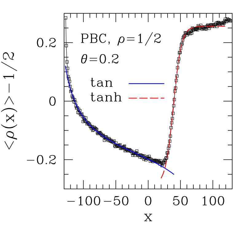
Figure 1: (Color online) Points give steady-state density profile for TASEP with hopping-rate gradient, for periodic boundary conditions, $\langle\rho\rangle=1/2$, lattice size $L=256$, and $\theta=0.2$ (see Eq. (1)). Full lines are fits to forms inspired by the theory of randomly-disordered systems (see text).

A schematic interpretation of the profile shape displayed in Figure 1 can be provided as follows, using ideas from previous treatments of the quenched random-bond version of the TASEP tb98 ; hs04 ; dqrbs08 . For the TASEP with uniform rates $p$, it is known derr98 ; sch00 ; derr93 ; be07 that, for currents greater or less than $J_{c}(p)=\frac{p}{4}$ the steady state phases are characterized by density profiles which are either: monotonically decreasing, $\langle\rho(x)\rangle-\frac{1}{2}=-q\,\tan q(x-x_{0})$ (high-current phase) or monotonically increasing, $\langle\rho(x)\rangle-\frac{1}{2}=k\,\tanh k(x-x_{0})$ (kink-like, low-current phase). Here, $q$ and $k$ are characteristic inverse lengths such that $q^{2}=-k^{2}=(J-J_{c})/4p$ derr93 ; hs04 ; mukamel , where $J$ is the steady-state current; the profile forms result from the fact that $J$ is constant throughout the system. This latter fact has strong bearing on the local shape of density profiles in the quenched random-bond case: in regions with weak (strong) bonds, i.e. bonds with low (high) hopping probability $p_{w}$ ($p_{s}$), $J$ can be larger (smaller) than the local critical current $J_{c}(p_{w})$ ($J_{c}(p_{s})$), in which case the profile is of high-current (low-current) type. With $\theta>0$ in Eq. (1), the features shown in Figure 1 appear roughly consistent with the theoretical framework just sketched. However, we shall see from the full treatment developed in Subsection II.2 below that, although the concepts of high- and low-current phases still persist here, their effects are strongly modified by factors specific to the present case. In particular, the separation in space of the two phases is actually very close to the left boundary in Figure 1, not where the tan and tanh functions join in the fit shown in that same Figure. This is because the actual profiles involve tan and tanh functions with spatially varying "envelope" factors (see Subsection II.2). Many new features will be seen to arise from the "registration" in space of the envelope, i.e. its position in the system; as we shall see, the location of the envelope relative to the region of weakest bonds is set by the current.

From the conjunction of PBC with the form of $p(x)$ given in Eq. (1), one sees that particles find a hopping-rate discontinuity of amplitude $-\theta$ as they jump across the chain’s endpoint. Although, from elementary considerations, PBC impose continuity of $\rho$ across the gap, it is important to emphasize that the kink-like profile seen in Figure 1 is not an artifact brought about by the discontinuity just mentioned. As we shall see in the following, kinks may (or may not) be present with PBC. Their existence, or lack thereof, depends on combinations of $\rho$ and $\theta$ according to mechanisms described by our theory.

One should note that, if the sign of $\theta$ is reversed in Eq. (1), the plot of $\langle\rho\rangle-1/2$ versus $x$ simply gets point-reflected relative to the origin.

The steady-state currents in the type of system studied here also differ markedly from their uniform counterparts. We recall that, for the latter with PBC, the relationship between current $J_{0}\equiv J(\theta=0,p,\rho)$ and density is

$$J_{0}=p\,\rho\,(1-\rho)\ ,$$ (2)

where $p$ is the uniform hopping rate. Eq. (2) is one example of relationships and quantities which mean field factorization gives exactly derr93 ; mukamel , and whose generalization for non-uniform rates is also exactly given by the generalized mean field theory developed here, as we shall see.

For now, we restrict ourselves to $\rho\leq\frac{1}{2}$ . The question of whether or not the $J-\rho$ diagram here displays the same symmetry, relative to $\rho=\frac{1}{2}$, as that for the uniform case will be discussed later, with help of the theory developed in Subsection II.2 . The effects on the current of a position-dependent $p(x)$ given by Eq. (1) are shown in Figure 2, for various densities, all of them not far removed from $\rho=1/2$. It is seen that as $\theta$ increases, the $J-\theta$ relationship becomes independent of $\rho$ for an increasingly broad range of densities, following the same nearly linear form as that of a system with $\rho=1/2$. In other words, for fixed $\theta$ a plateau develops around $\rho=1/2$ in the $J-\rho$ diagram, whose width increases with $\theta$ . Again, a similar effect is seen in TASEP with quenched randomness tb98 ; hs04  .

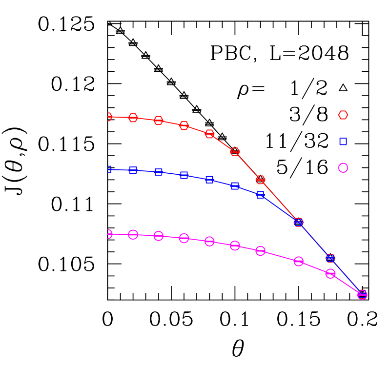
Figure 2: (Color online) Steady-state currents $J$ against gradient intensity $\theta$ for a system with $L=2048$ and PBC, for densities as shown. Each point is an average taken over $100$ independent samples, each in its turn containing $1.2\times 10^{6}$ successive steady-state configurations. Error bars are smaller than symbol sizes.

II.2 Mean-field theory

For uniform $p$, the Burgers equation fns77 ; vBks85 ; ks91 ; kk08 , linearized via the Cole-Hopf transformation hopf50 ; cole51 gives the general time-dependent mean field solution, analogous to a superposition of moving solitons, corresponding to waves in the linearized system, with possibly complex wave-vectors. Real and imaginary wave vectors distinguish the two general soliton-like steady states which, because of particle conservation, are uniform-current ones. These steady states correspond to phases of maximal current ($J\simeq J_{c}=p/4$) or low current ($0\leq J<J_{c}$, and low or high density); the square of the wave vector is proportional to $(J/J_{c}-1)$. For the special case of PBC, the two steady states become states of uniform density, while for open boundary conditions the steady state profiles are of tan and tanh form.

For space-dependent $p(x)$, the solution given below (for general time-dependence and then steady state) uses an adiabatic generalisation of constant-$p$ ideas.

We start from the continuity equation:

$$\frac{\partial\rho}{\partial t}=-\frac{\partial}{\partial x}\,J(x)\ ,$$ (3)

with (using a mean field factorization)

$$J(x)=p(x)\,\rho(x-\frac{1}{2})\,\left(1-\rho(x+\frac{1}{2})\right)\ ;$$ (4)

defining $\sigma$ via $\rho\equiv\frac{1}{2}(1+\sigma)$, Eq. (3) becomes, upon taking the continuum limit on Eq. (4):

$$2\,\frac{\partial\sigma}{\partial t}=\frac{\partial}{\partial x}\,\big{\{}p(x)\,[\sigma^{2}(x)+\frac{\partial\sigma}{\partial x}-1\,]\big{\}}\ .$$ (5)

Using the Cole-Hopf transformation hopf50 ; cole51 , we introduce the auxiliary variable $u$ via $\sigma=\partial\ln u/\partial x$, in terms of which, after a partial integration with respect to $x$, Eq. (5) turns into the linear form:

$$2\,\frac{\partial u}{\partial t}-f(t)\,u=p(x)\,\left\{\frac{\partial^{2}u}{\partial x^{2}}-u\right\}\ ,$$ (6)

where $f(t)$ is the integration "constant". Writing $u=X(x)\,T(t)$, one has

$$\frac{2}{T}\frac{dT}{dt}-f(t)=p(x)\left\{\frac{1}{X}\frac{d^{2}X}{dx^{2}}-1\right\}\equiv-\omega\ ,$$ (7)

whence

$$T=\exp(-\frac{1}{2}\omega t+F(t))\quad{\rm with}\quad\frac{dF}{dt}=\frac{1}{2}f(t)\ .$$ (8)

Putting

$$(\mu_{\omega}(x))^{2}\equiv 1-\frac{\omega}{p(x)}\ ,$$ (9)

and making the ansatz $X=e^{\gamma(x)}$, one gets

$$\frac{d\gamma}{dx}=\pm\mu_{\omega}(x)\ ,$$ (10)

provided $d\mu_{\omega}(x)/dx\ll(\mu_{\omega}(x))^{2}$ (adiabatic approximation). In this limit $X=e^{\pm\gamma_{\omega}(x)}$, with $\gamma_{\omega}(x)=\int^{x}\mu_{\omega}(x)\,dx$. Thus,

$$XT=\exp(\pm\gamma_{\omega}(x)-\frac{1}{2}\omega t+F(t))\ .$$ (11)

The general solution for $u(x,t)$ is

$$u=\sum_{\omega}A_{\omega}\cosh\left(\gamma_{\omega}(x)-\gamma_{\omega}(a_{\omega})\right)\,e^{-\frac{1}{2}\omega t+F(t)}\ ,$$ (12)

where the $A_{\omega}$ and $a_{\omega}$ are arbitrary constants. Finally, in terms of $\sigma(x,t)$:

$$\sigma(x,t)=\frac{\sum_{\omega}A_{\omega}\,\mu_{\omega}(x)\sinh\left(\gamma_{\omega}(x)-\gamma_{\omega}(a_{\omega})\right)\,e^{-\frac{1}{2}\omega t}}{\sum_{\omega}A_{\omega}\cosh\left(\gamma_{\omega}(x)-\gamma_{\omega}(a_{\omega})\right)\,e^{-\frac{1}{2}\omega t}}\ ,$$ (13)

in the mean field/adiabatic approximation.

The following comments are in order:

(i) If we take a single component in Eq. (13) the $e^{-\frac{1}{2}\omega t}$ factor cancels and we are left with a steady state solution:

$$\sigma(x)=\mu_{\omega}(x)\tanh\left(\gamma_{\omega}(x)-\gamma_{\omega}(a)\right)\ .$$ (14)

When the validity criterion for the adiabatic approximation applies, this state is associated with the current

$$J=\frac{1}{4}\,p(x)(1-\mu_{\omega}(x)^{2})=\frac{1}{4}\omega\ ,$$ (15)

[ using Eqs. (4), (9), and (14) ], which is constant as necessary for the steady state.

(ii) In the $t$-dependent general form Eq. (13), each sum evolves for long times into a single component, which is the one having the least $\omega$, corresponding to the steady state, i.e., $\omega=4J$ , by (i).

(iii) At long but not infinite times the sums in Eq. (13) are dominated by the terms with the smallest $\omega$’s. Then the denominator, whose logarithmic derivative gives $\sigma$, becomes a combination of the steady state component and a wave packet whose group velocity $v(x)$ can be obtained by a straightforward adiabatic generalisation of standard procedures, using the analogue $d\mu_{\omega}(x)/dx$ of the wave vector. The result is, generally,

$$v(x)=\pm p(x)\left(1-\frac{\omega}{p(x)}\right)^{\frac{1}{2}}\ ,$$ (16)

becoming $v(x)=\pm p(x)^{\frac{1}{2}}(p(x)-4J)^{\frac{1}{2}}$ for the kink dynamics in the late-time approach to the steady state.

In what follows we shall be mostly concerned with the steady state, so the following distinctions and details may be helpful. In Eq. (15),

$$J_{c}(x)\equiv\frac{1}{4}\,p(x)$$ (17)

acts like a local critical current, since the sign of $J-J_{c}$ determines whether $\mu(x)$ there is real or imaginary and, consequently, whether the profile in Eq. (14) involves a tanh or tan function. This is a generalization of the case with space-independent rate $p$, where $J_{c}=p/4$ is the maximal current, associated to flat or $\tan$ profiles, while low currents $J<J_{c}$ exhibit $\tanh$ profiles.

For the space-dependent $p(x)$ the most important new features are the $x$-dependence of $J_{c}(x)$, the $J$-dependent location ($x_{0}$) of the division between phases, and the occurrence of the space-dependent amplitude function $\mu(x)$ in the profile, Eq. (14). Where it is necessary, to avoid confusion, we distinguish the possibilities by using, in place of $\mu(x)$, the specific real functions $k(x)$, $q(x)$ defined by

$$k(x)=\mu(x)=(1-4J/p(x))^{\frac{1}{2}}=(1-J/J_{c}(x))^{\frac{1}{2}}\ ,$$

$$J<J_{c}(x)\ ;\quad$$

$$q(x)=i\,\mu(x)=(4J/p(x)-1)^{\frac{1}{2}}=(J/J_{c}(x)-1)^{\frac{1}{2}}\ ,$$

$$J>J_{c}(x)\ .\quad$$ (18)

Then

$$\sigma(x)=k(x)\,\tanh(K(x)-K(a)),\quad J<J_{c}(x)\ ;\$$

$$\sigma(x)=-q(x)\,\tan(Q(x)-Q(b)),\quad J>J_{c}(x)\ ,\$$ (19)

where $K(x)=\int^{x}k(x)\,dx$ and $Q(x)=\int^{x}q(x)\,dx$. For $x$-dependent rates, the $\tan$ form can only apply in at most a very limited region (of size set by the weakest rates). This is because the $\tan$ function in $\sigma(x)$ diverges, violating the physical requirement on the local density, $|\sigma(x)|\leq 1$, unless its argument $Q(x)$ is limited to a range less than $\pi$. So the $\tanh$ form will actually account for most of the profile. If the integration constant $a$ is inside the system the change of sign of the argument of the $\tanh$ function at $x=a$ corresponds to a kink there. For the $\tanh$, $k(x)$ acts like an envelope, and its crucial effects in distinguishing scenarios and phases partly relate to its registration, for which the $\tan$ part of the profile can play a dominant role.

III Steady State with PBC

III.1 Introduction

For the non-uniform system with $x\in[-L/2,L/2]$, PBC impose the constraint on $\sigma(x)$:

$$\sigma\left(-L/2\right)=\sigma\left(L/2\right)\ .$$ (20)

In addition to this, in order to fix arbitrary constants and determine the steady state current $J$ and profile $\sigma(x)$, we need also to specify the average density $\langle\rho\rangle$, in the equation

$$2\,(\langle\rho\rangle-\frac{1}{2}\,)=\langle\sigma\rangle=\frac{1}{L}\,\int_{-L/2}^{L/2}\sigma(x)\,dx\ .$$ (21)

With the mean field/adiabatic approximation this becomes

$$\langle\sigma\rangle=\frac{1}{L}\,\int_{-L/2}^{L/2}\mu(x)\tanh\left(\gamma(x)-\gamma(a)\right)\,dx=$$

$$=\left[\ln\cosh\left(\gamma(x)-\gamma(a)\right)\,\right]_{-L/2}^{L/2}\ .$$ (22)

Here we used $\mu=d\gamma/dx$, and have reverted to non-specific notation, not distinguishing $\tanh$ or $\tan$ (nor $\cosh$ or $\cos$). We will later have to verify that the criterion for use of the adiabatic approximation is satisfied.

From the general formulation above, $\mu$ and hence $\gamma$ are related to the current $J$; it and the other parameter $a$ (the kink position in the case of real $\gamma(a)$) are determined in terms of $\langle\rho\rangle$ by Eqs. (21) and (22) (for large systems, the kink position will be sharp when the adiabatic approximation is satisfied) .

III.2 Rate gradient

From now on we deal with the specific case of linearly-varying $p(x)$ given in Eq. (1) . With PBC and $\theta\geq 0$, one gets in the adiabatic approximation, with the help of Eqs. (9), (10), and (15):

$$\mu(x)=\left[1-\frac{4J}{p(x)}\,\right]^{\frac{1}{2}}=\left[\frac{X}{X+c}\,\right]^{\frac{1}{2}}\ ,$$ (23)

and

$$\gamma=\int^{x}\mu(x)\,dx=[X(X+c)]^{\frac{1}{2}}-c\tanh^{-1}\left[\frac{X}{X+c}\right]^{\frac{1}{2}}$$

$$\equiv{\widetilde{K}}(X)\ ,\qquad\quad$$ (24)

where

$$X=x-x_{0}\ ,\qquad\qquad\qquad\qquad\quad$$

$$x_{0}=(8J-1)\,\frac{L}{2\theta}\equiv-\lambda\,\frac{L}{2}\ ;\qquad\qquad$$

$$c=\frac{4JL}{\theta}=x_{0}+\frac{L}{2\theta}=\frac{L}{2}\,\left(\frac{1}{\theta}-\lambda\right)\ .$$ (25)

$x_{0}$ corresponds to the place where $\mu(x)$ vanishes, hence to the position of the apex of the envelope function $\pm|\mu(x)|$, i.e., where $\mu(x)$ [ and $\gamma(x)\,$] cross over between real and imaginary values $k(x)$ or $-i\,q(x)$ [ and $K(x)$ or $-i\,Q(x)\,$]. Subsequently explicit forms will be needed, particulary for $\gamma$ for the real case, and it will then be convenient to use both $K$ and (real) $\widetilde{K}$, where

$$K(x)={\widetilde{K}}(X)\ ,$$ (26)

with $X=X(x)=x-x_{0}$, and where $\widetilde{K}$ is as in Eq. (24). $x_{0}$ also corresponds to the place where $J$ is equal to the local critical current; this plays a central role in the discussion. For graphical illustrations, refer to Figure 4 in subsection III.4 below. $c$ is a characteristic length related to the rate gradient. $\lambda$, the ratio of $x_{0}$ to $-L/2$, conveniently distinguishes scenarios, and parametrizes analytic expressions, particulary in the $L\to\infty$ limit.

III.3 Scenarios for steady state behavior

We next discuss the character and location of steady state phases, and relationships to positions of the "envelope" and kinks. The generalised maximal current and low current phases of the system turn out to be described by two scenarios, I and II, as follows.

For the rate gradient case with $\theta>0$ ($\theta<0$ has dual character), the smallest $p(x)$ is at the left-hand side edge, giving a severe bottleneck there. As we shall see in the following, this has the consequence that the current $J$ adjusts itself in such a way that the apex position $x_{0}=-\lambda L/2$ turns out to be either: (I) near the left boundary, but still inside the system, or (II) to the left of the left boundary. These give, respectively:

Scenario I: $\lambda\lesssim 1$. Here the $\tan$ function applies near the left edge and its spatial extent $\Delta x$ is limited by the condition $\Delta Q(x)=q(x)\,\Delta x<\pi$. Since $q(x)$ is related to the difference $J-J_{c}(x)$ of the steady state current $J$ from its local critical value, this condition also limits $J$ as well as the position, $x=x_{0}$, where $J-J_{c}(x)$ vanishes.

Scenario II: $\lambda>1$. Here only the $\tanh$ function applies inside the system.

The two scenarios become very evident in the "family" of profiles corresponding to all possible average densities $\langle\rho\rangle$, for PBC and a given $\theta$ (see the numerical results in Figure 4).

Scenario I corresponds to a common envelope (nearly parabolic in shape, see Eq. (23)) and applies for an intermediate range of $\langle\rho\rangle$’s (not very far from $1/2$). It is consistent with a fixed position $x_{0}$ of the apex of the envelope, close to the left hand boundary. It is (through Eq. (25)) consistent with an observed constant ($\langle\rho\rangle$-independent) plateau current $J$, about $(1/8)(1-\theta)$. Near the left boundary there is a small region of $\tan$ profile, and everywhere else the profile approaches the $\tanh$ form (including the kink).

Scenario II, applying for larger $|\langle\rho\rangle-1/2|$, has profiles not near a common envelope, corresponding to varying apex position; indeed, in this case $x_{0}$ is outside of the system (to the left of the left boundary) and the profile is entirely of $\tanh$ type. In this scenario the currents depend on $\langle\rho\rangle$.

These scenarios and related phenomena can be quantitatively explained using the mean field adiabatic formulation, except near the envelope apex if that lies inside the system. This is because the apex is where $\mu(x)$ vanishes, i.e., where the adiabatic approximation fails utterly (see the validity criterion, below Eq. (10)). To the right of the apex, where $J<J_{c}(x)$, the adiabatic approximation is valid for $X>c^{\,1/3}$, so the adiabatic form $\sigma_{R}=k(x)\,\tanh(K(x)-K(a))$ applies; similarly, in the region to the left of the apex, $J>J_{c}(x)$, and the adiabatic form $\sigma_{L}=-q(x)\,\tan(Q(x)-Q(b))$ is valid for $X<-c^{\,1/3}$ . Between these a (nonadiabatic) form $\sigma_{C}\propto(x+{\rm const.})^{-1}$ is adequate. So the profile can be a piecewise combination of $\sigma_{L}$, $\sigma_{C}$, and $\sigma_{R}$, except for scenario II, where only $\sigma_{R}$ applies.

In all cases, for the integral in Eq. (21) for ($2\langle\rho\rangle-1$) it turns out that at large $L$ the contribution from $\sigma_{R}$ dominates, and it alone gives the $L\to\infty$ value. This is because of the limitation of the range of the $\tan$ function in $\sigma_{L}$, to prevent its divergence, and of the range [$\,\sim\leavevmode\nobreak\ c^{1/3}\leavevmode\nobreak\ \propto\leavevmode\nobreak\ L^{1/3}\,$] of $\sigma_{C}$. This makes their contributions to the integral less than that from $\sigma_{R}$ by a factor which vanishes as $L$ increases.

Note that, quite generally, the limitation of $\sigma_{L}$ requires $x_{0}$ to satisfy $x_{0}-(-L/2)<\pi/q(-L/2)$; in the limit $L\to\infty$ this restricts the variable $\lambda$ defined above to the two possibilities $\lambda=1$ (envelope apex very near the left boundary) or $\lambda>1$ (apex [well] outside). These are respectively Scenarios I and II, whose details are now exhibited.

III.3.1 Scenario I

In this case, where $\lambda=1$, we investigate its quantitative character and which values of $\langle\rho\rangle$ and $J$ are consistent with it. Firstly, from Eq. (25), $\lambda=1$ makes $J=(1/8)(1-\theta)$. For possible values of $\langle\rho\rangle$, we consider Eqs. (21) and (22). We chose the integration constant $a$ so that $x=a$ is the center of the kink. If the kink is inside the system, the further it is to the right the smaller will be the integral, and the associated $\langle\rho\rangle-1/2$. There is clearly a least $\langle\rho\rangle$ in Scenario I, applying when the kink is as far to the right as it can be (consistent with PBC). But Scenario II allows displacement of the envelope to the left ($\lambda>1$), and with fixed kink position this affects the value of the integral, since the more the envelope is displaced to the left, the larger will be the amplitude $k(x)$ of the $\tanh$ at any particular $x$ inside the system.

So, small $|\langle\rho\rangle-1/2|$ can be achieved with envelope apex near the left hand boundary, by adjusting the kink position (Scenario I), while $\langle\rho\rangle$ nearer $0$ or $1$ needs a large displacement (${\cal O}(L)$) of the envelope to the left, corresponding to $\lambda>1$ (Scenario II).

For illustration, consider the special case $\langle\rho\rangle=1/2$ for which the numerical profile is actually shown in Fig.1. In the Figure it is evident that the required zero value of the integral between the profile curve and the $x$-axis is achieved by having the abrupt rise of the curve, corresponding to the kink, where it is. To the right(left) of the kink the curve follows the upper (lower) branch of the envelope function ($k(x)$ is monotonically increasing). At the extreme left is the region around $x_{0}$ (necessarily small) where the $\tanh$ has become $\tan$; its near divergence makes it easily able to match the PBC requirement. Thus one sees, in retrospect, that the fit shown in Fig.1 is in fact quite misleading.

Scenario I is consistent as long as the kink stays within the right boundary of the system. Then, $\sigma(L/2)$ at that boundary is positive and the PBC requiring $\sigma(-L/2)$ to have the same positive value can be readily satisfied, as the $\tan$ form needs only a very small adjustment of its argument (within $\approx\pi$) to achieve this. At the same time the spatial range in which the $\tan$ form applies has to be very small to prevent unphysical $\sigma_{L}$’s . Of course $\sigma_{L}$ and $\sigma_{C}$, and the relationship of their constants to $a$ are needed to complete the determination of the profile.

This discussion is easily generalized and made more quantitative by using the integration result in Eq. (22), with the appropriate real version $K(x)$ of $\gamma(x)$, together with the fact that when the kink at $X=a-x_{0}\equiv A$ lies well inside the system ${\widetilde{K}}(X)-{\widetilde{K}}(A)$ is large (${\cal O}(L)$) at both limits, but of opposite signs. Further, the kink width ($\equiv w$), such that the argument of $\tanh$ in Eq. (22) changes by ${\cal O}(1)$ between $x=a\pm w/2$, is $w\approx[d{\widetilde{K}}(A)/dA]^{-1}=[(A+c)/A]^{1/2}$, which is ${\cal O}(1)$ for $a={\cal O}(L)$, except near $x_{0}$ where $w$ diverges. Hence the integration result is, in the limit of large $L$,

$$2\,(\langle\rho\rangle-\frac{1}{2}\,)=\frac{1}{L}\,\left({\widetilde{K}}(L)-2{\widetilde{K}}(A)\right)\ ,$$ (27)

where

$${\widetilde{K}}(X)=[X(X+c)]^{1/2}-c\tanh^{-1}\left[\frac{X}{X+c}\right]^{1/2}\ .$$ (28)

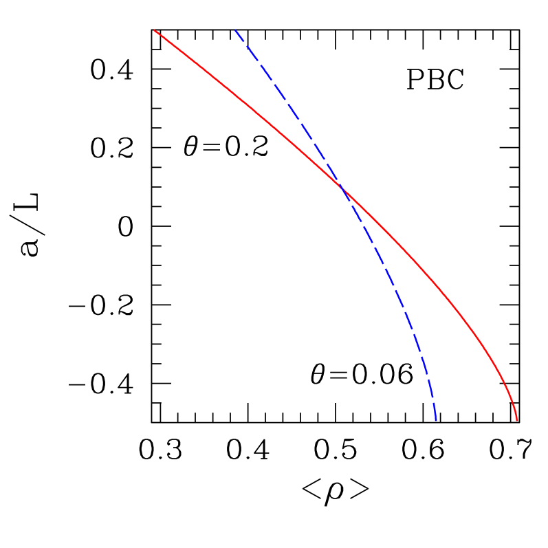
Figure 3: (Color online) Kink position $a/L$ against density $\langle\rho\rangle$ [ see Eqs. (27) and (28) ], for systems with PBC and rate-gradient values $\theta$ as shown.

For the special case $\langle\rho\rangle=1/2$ the kink position then has to be such that ${\widetilde{K}}(A)=(1/2){\widetilde{K}}(L)$ which, using the explicit form of $\widetilde{K}$ [ see Eqs. (26) and (28) ], gives $A/L=(1/2)+a/L\approx 0.61$ for $\theta=0.2$, consistent with the kink position in Figure 1. The general solution for the kink position against particle density is exhibited in Figure 3, for illustrative values of $\theta$. Note that the range of values of $\langle\rho\rangle$ for which solutions are found is symmetric relative to $\langle\rho\rangle=1/2,$ and gets broader with increasing $\theta$ [ see also Eq. (29) below ].

Larger values of $a$ are associated, through Eq. (22), with $\langle\rho\rangle<1/2$, up to the limit $a=L/2$ when the kink center is at the right boundary. Then the mean density takes the limiting value $\langle\rho\rangle_{c}$ such that

$$(\langle\rho\rangle_{c}-\frac{1}{2}\,)=-\frac{1}{2L}\,{\widetilde{K}}(L)=\qquad\qquad\quad$$

$$=\frac{1}{4}\{[2(1+\frac{1}{\theta})]^{1/2}-(\frac{1}{\theta}-1)\tanh^{-1}\left[\frac{2\theta}{1+\theta}\right]^{1/2}\}\ .\qquad$$ (29)

This marks the condition where the two scenarios meet, and will correspond to the limit of a plateau region (in which, for $L\to\infty$, $J=\frac{1}{8}(1-\theta)$ applies) in the "fundamental" diagram relating $J$ with $\langle\rho\rangle$ and $\theta$.

At $\langle\rho\rangle>1/2$ one finds equations identical in form to Eq. (27), (28), and (29), with $\frac{1}{2}-\langle\rho\rangle$ replacing $\langle\rho\rangle-\frac{1}{2}$. For small $\theta$, Eq. (29) gives $\langle\rho\rangle_{c}-1/2=-(\sqrt{2}/3)\,\theta^{\,1/2}$. Thus, the extent of the plateau in the $J-\langle\rho\rangle$ diagram vanishes as $\theta\to 0$. In this limit, for $\langle\rho\rangle$ still within the plateau, one can show that the height of the kink vanishes as $\theta^{1/2}$.

III.3.2 Scenario II

Scenario II applies at $\langle\rho\rangle$’s so small (for a given $\theta$) that the kink center is beyond the right boundary of the system (see, e.g., the curves for $\langle\rho\rangle=0.25$, $0.125$ in Figure 4). Then the apex position $x_{0}$ of the $\tanh$ envelopes has to go outside of the system on the left, and there has to be a small upturn in $\sigma$ at the extreme right of the system to satisfy the PBC, so the start of the kink is just visible there in Figure 4, and the kink center is actually beyond the right boundary. This means that the $\tanh$ profile applies throughout the system:

$$\sigma(x)=\sigma_{R}=k(x)\,\tanh(K(x)-K(a))\ ,$$ (30)

where $K(x)$ is again as in Eqs. (24) and (26). We will now have $x_{0}<-L/2$ and $L/2<a<L/2+w$, where $w$ is the kink width (of order $1$).

As discussed above, for given $\theta$ specifying $\langle\rho\rangle<\langle\rho\rangle_{c}<1/2$ [ see Eq. (29) ] will lead to $x_{0}/L<-1/2$, so making $J<(1/8)(1-\theta)$ and $\lambda>1$. As before, we use Eqs. (22) and (24). But now, since $x_{0}<-L/2$, and for all $x$ in the system $x<a$, ${\widetilde{K}}(x)-{\widetilde{K}}(a)$ is at both limits negative (and large). So we have [ ignoring contributions to $2(\langle\rho\rangle-1/2)\,L$ of lower order in $L$ (from corrections to the adiabatic approximation, and from width of the kink), and the comparable small distance the center lies beyond the right boundary ]:

$$2(\langle\rho\rangle-\frac{1}{2})\approx\frac{1}{L}\{\,{\widetilde{K}}(\frac{L}{2}(\lambda+1))-{\widetilde{K}}(\frac{L}{2}(\lambda-1))\,\}$$ (31)

where ${\widetilde{K}}(X)$ is as in Eq. (28). This gives $\lambda$ in terms of $\langle\rho\rangle$ and $\theta$, for $\langle\rho\rangle$ less than the critical value, and hence provides the following current-density relation outside of the plateau region

$$J=\frac{1}{8}\,(1-\lambda\theta)\ ,$$ (32)

with

$$4\,(\frac{1}{2}-\langle\rho\rangle)=[(\lambda+1)(\frac{1}{\theta}+1)]^{\frac{1}{2}}-[(\lambda-1)(\frac{1}{\theta}-1)]^{\frac{1}{2}}-$$

$$-(\frac{1}{\theta}-\lambda)\,\{\tanh^{-1}\left[\frac{\lambda+1}{\theta^{-1}+1}\right]^{\frac{1}{2}}-\tanh^{-1}\left[\frac{\lambda-1}{\theta^{-1}-1}\right]^{\frac{1}{2}}\}\ .$$

(33)

A similar procedure applies for the complementary subcase, $(1-\langle\rho\rangle)<\langle\rho\rangle_{c}<1/2$, by particle-hole duality.

Eqs. (32) and (33) can be combined to give $J$ as a function of $\langle\rho\rangle$ in Scenario II, for fixed $\theta$. The range of values of $\langle\rho\rangle$ for which physically acceptable solutions are found is complementary to that limited by Eq. (29), which marks the extremes of validity of Scenario I.

III.3.3 Weak-bond interpretation of plateau current

Before moving to numerical results, we introduce an additional piece of mean-field theory which will be useful later.

As remarked above, a plateau current, similar to that predicted in Scenario I, is found in the TASEP with random rates $p(x)$ tb98 ; hs04 ; dqrbs08 . There, an interpretation is given in terms of the current limitation provided by the weakest bonds, $p_{w}$, which suggests that the "maximal" current satisfies $J_{\rm max}\leq p_{w}/4$. The following generalization provides a direct interpretation and confirmation of the result $J_{\rm max}=\frac{1}{8}(1-\theta)$ predicted for the plateau phase in Scenario I.

In the continuum mean field formulation, Eqs. (3), (4), and (5) give for all $x$:

$$J=\frac{1}{4}\,p(x)\,\{1-\sigma^{2}(x)-\frac{\partial\sigma}{\partial x}\}\ .$$ (34)

The most limiting rate, occurring at $x=-L/2$, is $p_{w}=\frac{1}{2}\,(1-\theta)$, so $J_{\rm max}$ is obtained from applying Eq. (34) there. In Scenario I, with $\lambda=1$, the $\tan$ solution Eq. (19) applies in that region [ i.e. $X={\cal O}(1)\,$], which yields for the right-hand side of Eq. (34), using Eqs. (18), (23), and  (25):

$$\frac{1}{4}\,p_{w}\,(1+q^{2})=\frac{1}{4}\,p_{w}\,\{1-\frac{X}{X+c}\}=\frac{1}{4}\,p_{w}\,\{1+{\cal O}(\frac{1}{L})\}\ ,$$ (35)

hence confirming the infinite-system maximal current $\frac{1}{8}\,(1-\theta)$.

III.4 Numerical results

We considered lattices with $L=2^{m}$ sites, $8\leq m\leq 13$. A time step is defined as a set of $L$ sequential update attempts, each of these according to the following rules: (1) select a site at random; (2) if the chosen site, here denoted by $x$, is occupied and its neighbor to the right is empty, then (3) move the particle with probability $p(x)$. Thus, in the course of one time step, some sites may be selected more than once for examination, and some may not be examined at all.

We have found that the time needed to attain steady-state flow varies roughly with $L^{3/2}$, similarly to the uniform-rate case dqrbs08 , for which this is well-known fns77 ; gwa ; dhar , and is in agreement with the correspondence between the (uniform) TASEP and evolution of a KPZ interface ks91 ; kk08 ; kpz ; meakin86 .

For density profiles, local densities were usually averaged over snapshots (taken at appropriately long times) of $10^{4}$ independent samples. For example, for $L=256$ we found that steady state has been reached by time $t=10^{4}$ in most cases, except for points on the coexistence line for open BCs (see Section IV) where the approach to stationarity is markedly slower. Although finite-size effects can be observed, they are generally small and act towards making any kinks sharper, relative to system size, without any qualitative change. Thus we can be confident that no significant physical features are missed by generally exhibiting profiles corresponding only to $L=256$, as done here.

Figure 4 shows steady-state density profiles for $\theta=0.2$, which although still in the scaling regime is a relatively steep gradient. The behavior is in full agreement with the theory developed in Subsection II.2: (i) according to Scenario I, there is a common envelope, pinned to the left-hand extreme of the system, for intermediate densities roughly between $0.3$ and $0.7$; (ii) within this range of densities a kink is present, whose location varies against $\langle\rho\rangle$ as predicted by Eqs. (27) and (28); (iii) for densities further removed from $1/2$, Scenario II takes over, and profiles follow either the lower branch of the envelope (with its $\langle\rho\rangle$- dependent displacement) with an incipient kink at the right boundary (for $\langle\rho\rangle<1/2$), or the upper branch, in this case with a narrow downward turn at the left edge in order to satisfy PBC ($\langle\rho\rangle>1/2$).

Envelope functions are already familiar in the profiles of constant-rate asymmetric exclusion processes (e.g., on the coexistence line), but they only involve new scenarios when their delimitation of density profiles is space-dependent (as above or, e.g., in asymmetric exclusion problems with Langmuir dynamics pff04 ).

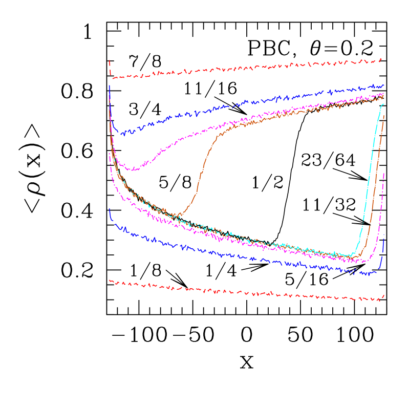
Figure 4: (Color online) Steady-state local density profiles for system with $L=256$ and PBC, $\theta=0.2$. Curve labels denote average particle densities.

There are slight numerical discrepancies between predictions of Subsection II.2 and the data displayed in Fig. 4, which exemplify the finite-size effects referred to above. For instance, according to Eqs. (27), (28), and (29) [ see also Fig. 3 ], for $\theta=0.2$ Scenario I should hold for $0.293\dots\leq\langle\rho\rangle\leq 0.707\dots$. However, the profile for $\langle\rho\rangle=5/16=0.3125$ already shows some deviation from the common envelope. Overall, we have found that the quantification of finite-system corrections, together with accurate analysis and extrapolation to the $L\to\infty$ limit, can best be accomplished when dealing with steady-state currents, as shown in the following.

Evaluation of steady-state currents involved averaging over $N_{s}=100$ independent samples, for each of which $N_{c}=a_{L}\,L^{3/2}$ successive instantaneous current values were accumulated. We took $a_{L}\approx 130$ for $L=256$ and $512$, and $\approx 13$ for larger $L$. The instantaneous current is $n_{\rm moves}/L$, where $n_{\rm moves}$ is the number of particles which undergo successful move attempts in the course of a unit time interval, i.e., $L$ stochastic site probings as defined above. As is well known dqrbs96 , the width $\delta J$ of the distribution thus found is essentially independent of $N_{s}$ as long as $N_{s}$ is not too small, and varies as $N_{c}^{-1/2}$. With the parameters as specified here, we managed to keep $\delta J$ well below the finite-size difference between $J$ estimates for consecutive values of $L$ (for fixed $\theta$, $\rho$). The relevance of finite-size effects for currents is illustrated for $\rho=1/2$ in Fig. 5, where $\theta$ is restricted to small values for clarity of presentation; one can see that the curvature present in finite-$L$ data is essentially absent upon extrapolation to $L\to\infty$.

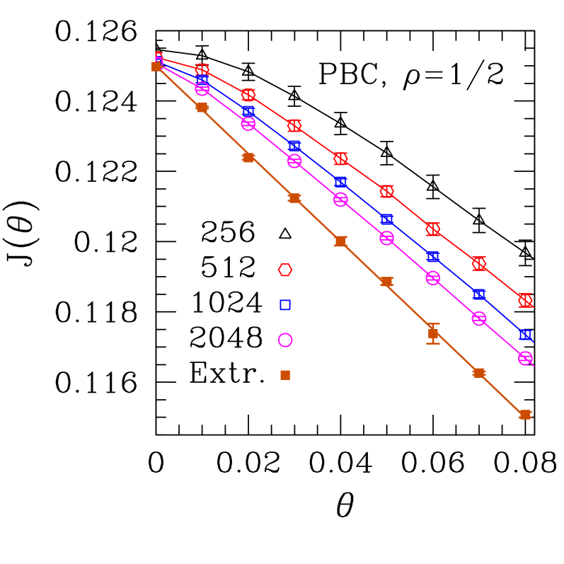
Figure 5: (Color online) Steady-state currents $J$ against gradient intensity $\theta$ for $\rho=1/2$ and PBC, for system sizes as shown, plus extrapolated curve; for details of extrapolation, see text.

We now discuss guidelines for extrapolation of finite-system currents $J_{L}$ to their thermodynamic-limit value $J_{\infty}$.

In line with general finite-size scaling ideas, we attempted single-power fits of our sequences of finite-$L$ current data with an adjustable finite-size scaling exponent $\psi$, for all available pairs $\theta$ and $\rho$. We denote by $\theta_{c}(\rho)$ the gradient intensity value above which $J(\rho,\theta)$ becomes independent of $\rho$.

So, $\theta<\theta_{c}(\rho)$ corresponds to Scenario II of Subsection III.3 above, while $\theta>\theta_{c}(\rho)$ is associated with Scenario I. Although $\theta_{c}$ still carries an $L$-dependence (thus, e.g., the mergings of $J-\theta$ curves shown in Fig. 2 take place at slightly different locations for $L\neq 2048$), it is a rather small effect compared to the overall range of $\theta$-variation investigated.

Results were as follows:

(1) For $0\leq\theta\lesssim\theta_{c}(\rho)$, $\psi\approx 1$ (Scenario II);

(2) For $\theta\gtrsim\theta_{c}(\rho)$, $\psi\approx 1/2$ (Scenario I).

In the immediate vicinity of $\theta_{c}(\rho)$, on both sides, we had rather serious convergence issues, so there we generally resorted to fixing $\psi=1/2$, for which the corresponding extrapolations fell in smoothly with the remaining ones outside that interval. For region (2), we estimate the uncertainty for $\psi$ to be of order $10\%$ at most.

Thus, for the extrapolated points in Fig. 5, $\psi\in(0.45,0.55)$ was found in all cases except that corresponding to $\theta=0$, for which $\psi\approx 1$. The case of $\langle\rho\rangle=1/2$ shown in that Figure is somewhat exceptional in that, as remarked at the end of Subsection III.3.1 above, there the extent of validity of Scenario II corresponds only to the limit $\theta\to 0$.

In Fig. 6 below we present the set of extrapolated currents for $\rho=1/2$, corresponding to $0\leq\theta\leq 0.2$, together with the mean-field prediction of a straight line $J_{\rm MF}(\theta)=\frac{1}{8}\,(1-\theta)$  for Scenario I (see also the weak-bond interpretation given in Subsec. III.3.3). The agreement is remarkable.

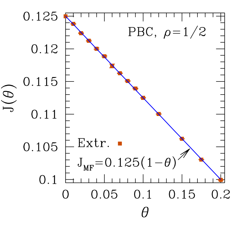
Figure 6: (Color online) Points are extrapolated currents for system with $\rho=1/2$, PBC. Full line is the mean-field approximation (see text).

Considering now the extrapolated currents for $\langle\rho\rangle\neq 1/2$, one sees in Fig. 7 that the variation of $J$ against $\theta$ is generally much slower where Scenario II holds. In the vicinity of $\theta_{c}(\rho)$, due to the convergence issues mentioned above, we considered systems of sizes up to $L=8192$ (away from that region, we found that using $L\leq 2048$ was generally enough to distinguish a reliably smooth trend as $L^{-1}\to 0$). Upon extrapolation we found the small overshoots shown in the Figure, which when translated to $J-\langle\rho\rangle$ diagrams for fixed $\theta$, would amount to reentrant behavior. For the largest deviation found, corresponding to $\rho=5/16$ at $\theta=0.175$, one gets $J=0.1039(1)$, while the value for $\rho=1/2$ at the same $\theta$ is $0.1030(1)$. Although the average values differ by just under $1\%$, when converted in terms of (estimated) uncertainties this difference is equivalent to nine error bars. So, this effect appears to be real.

The data in Fig. 7 can be used to test Eq. (29). In order to do so, for fixed $\langle\rho\rangle<1/2$ one needs to establish the boundary between the ranges of validity of Scenarios I and II, as given by numerical simulations. Due to the overshoots just referred to, this task carries some ambiguity. For simplicity, we assumed such location to be where the respective $J-\theta$ curve first crosses that for $\langle\rho\rangle=1/2$, upon increasing $\theta$. Fitting the data thus obtained to the form $\frac{1}{2}-\langle\rho\rangle=a\,\theta^{b}$, one finds $a=0.471(4)$, $b=0.51(1)$. These are to be compared, respectively, to $a=\sqrt{2}/3=0.4714\dots$, $b=1/2$, from the small-$\theta$ expression of Eq. (29) (see paragraph below that Equation). Thus, the above assumption seems justified.

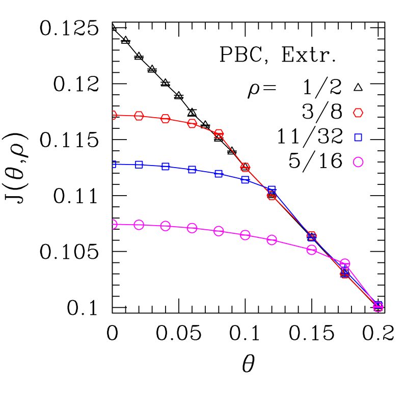
Figure 7: (Color online) Extrapolated steady-state currents versus gradient intensity for systems with PBC, and densities as shown. Note overshoots.

Furthermore, data within the region of validity of Scenario II can be compared with the predictions of Eqs. (32) and (33). We used $\theta=0.06$. One sees in Fig. 8 that the agreement between theory and extrapolated numerical results is indeed excellent. The prediction of a plateau for Scenario I is also borne out by numerics, within error bars. One cannot see unequivocal evidence here for a reentrant behavior similar to that found in Fig. 7. It is possible that such an effect, if present, is smaller than for the cases depicted in the latter Figure. This would be in line with the observation that the amplitude of the reentrance decreases with decreasing $\theta$ .

Fig. 8 also shows the $J-\langle\rho\rangle$ relation for uniform hopping-rate systems, for comparison.

A current-density diagram very similar to Fig. 8 was obtained in Ref. lak06, , for the partially asymmetric exclusion problem with spatially-varying hopping rates.

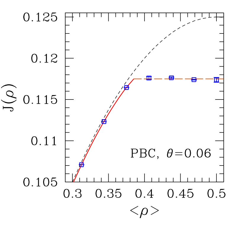
Figure 8: (Color online) Points are extrapolated ($L\to\infty$) steady-state currents; full line is $J-\langle\rho\rangle$ relationship from Eqs. (32) and (33) [ Scenario II ]; long-dashed horizontal line is $J=0.1175$, from Eq.(25) with $\lambda=1$ [ Scenario I ]. Short-dashed line is $J-\langle\rho\rangle$ relationship for uniform hopping-rate systems, Eq.(2).

IV Open boundary conditions

IV.1 Introduction

With open boundary conditions, the following additional quantities are introduced: the injection (attempt) rate $\alpha$ at the left end, and the ejection rate $\beta$ at the right one. Calling $\rho_{L}$, $\rho_{R}$ the stationary densities respectively at the left and right ends of the chain, one has for the current $J$ at the boundaries, and anywhere inside:

$$\alpha\,(1-\rho_{L})=J=\beta\,\rho_{R}\ .$$ (36)

Scenarios I and II, regarding the existence and location of an "envelope", discussed in the preceding section, still apply here, with similar consequences upon the system-wide current. The overall picture turns out to be rather like that for open systems with uniform hopping rate derr98 ; sch00 ; derr93 ; ds04 ; rbs01 ; be07 ; nas02 ; ess05 : a maximal-current phase arises for suitably large $\alpha$, $\beta$ (where Scenario I takes hold); elsewhere, one has less-than-maximal current, although with either low or high density, the latter two subphases being separated by a coexistence line; Scenario II applies. See Fig. 9 and corresponding insets.

The robustness of the three-phase structure in the present case is in line with the results of Ref. lak06, . In their study of the partially asymmetric exclusion problem, with spatially-varying right- and left- hopping rates $p(x)$ and $q(x)$ respectively, those authors always found three phases, as long as $p(x)-q(x)$ did not change sign.

In the maximal current phase, the following specific features are noteworthy:

(i) the steady-state system-wide density $\langle\rho\rangle$ is very close to the value which, for PBC, corresponds to the lower limit of validity of Scenario I. This is because, from the conditions given in Eq. (36), for large $\alpha,\beta$ one must have $\rho_{L}$ "large" and $\rho_{R}$ "small". Thus the density profile essentially follows the lower branch of the envelope function. Slight departures from that occur within short ("healing") distances from the extremes, in order to comply with the exact values dictated by Eq. (36). The latter effects account for the fact that $\langle\rho\rangle$ is not strictly constant throughout the maximal-current phase. Although Eq. (36) imposes the same constraints for systems with uniform hopping rates, there the envelope is trivially $x-$independent, and $\langle\rho\rangle$ is close to $1/2$ sch00 ; mukamel ; rbs01 .

(ii) In contrast to Scenario I with PBC, the steady-state profiles here do not show a kink inside the system.

(iii) Similarly to Scenario I with PBC, the $\tan$- like segment of the profile at the extreme left of the system is essential in the local density adjustment near that edge. However, as just mentioned, such adjustment is here imposed by Eq. (36), as opposed to the former case where the constraint arises from demanding continuity of $\rho$ to obey PBC (combined with the existence of a kink further to the right).

IV.2 Theory and Scenarios

In the "low current" Scenario II, with the apex left of the system’s left boundary ($x_{0}=-\lambda\,L/2$, with $\lambda>1$), one has only $\tanh$ type solutions for all $x$; $\sigma=2(\langle\rho\rangle-\frac{1}{2})$ is limited by the envelope $\pm k(x)$:

$$k(x)=\left[1-\frac{4J}{p(x)}\right]^{1/2}=\left[\frac{(2\theta/L)(x-x_{0})}{1+(2\theta/L)\,x}\right]^{1/2}\ .$$ (37)

So,

$$J=\frac{p(x)}{4}\,(1-k^{2}(x))=\frac{1}{8}\left(1+\frac{2\theta}{L}\,x\right)\,(1-k^{2}(x))\ .$$ (38)

Taking $x=x_{0}$, where $k(x_{0})=0$, gives

$$J=\frac{1}{8}\,(1-\lambda\,\theta)\ ,$$ (39)

while evaluating Eq. (37) at $x=\mp L/2$ gives

$$k_{L,R}=k(\mp\frac{L}{2})=\left[\frac{\theta(\lambda\mp 1)}{1\mp\theta}\right]^{1/2}\ ,$$ (40)

which sets the upper ($\rho_{L,R}^{>}$) and lower ($\rho_{L,R}^{<}$) bounds for the density at the extremes:

$$\rho_{L,R}^{>,<}=\frac{1}{2}\left(1\pm k_{L,R}\right)\ .$$ (41)

With $\sigma(x)=k(x)\,\tanh(K(x)-K(a))$, where $x=a$ is the position of the kink, and $K=\int k(x)\,dx$, one can see from the insets in Fig. 9 that, considering the situations corresponding to profiles types (i), (ii), and (iii) shown there, the following constraints hold:

$$\begin{cases}{\rho_{L}^{<}\leq\rho_{L}\leq\rho_{L}^{>}\qquad\quad\ {\rm(i)}}\cr{\rho_{L}=\rho_{L}^{<}\qquad\quad\qquad{\rm(ii),(iii)}}\end{cases}\ ;$$

$$\noindent\begin{cases}{\rho_{R}=\rho_{R}^{>}\qquad\qquad\quad{\rm(i),(ii)}}\cr{\rho_{R}^{<}\leq\rho_{R}\leq\rho_{R}^{>}\qquad\quad{\rm(iii)}}\end{cases}\ .$$ (42)

So, using Eqs. (36) and (38) we obtain, for the possible values of $\alpha$ and $\beta$ in the three situations:

$$\alpha_{\rm(i)}\in\left[\frac{J}{1-\rho_{L}^{<}}\,,\,\frac{J}{1-\rho_{L}^{>}}\right]=\frac{1}{4}(1-\theta)\,\left[1-k_{L},1+k_{L}\right]\ ;$$

$$\alpha_{\rm(ii),(iii)}=\frac{J}{1-\rho_{L}^{<}}=\frac{1}{4}(1-\theta)\,(1-k_{L})\ ;$$

$$\beta_{\rm(i),(ii)}=\frac{J}{\rho_{R}^{>}}=\frac{1}{4}(1+\theta)\,(1-k_{R})\ ;$$

$$\beta_{\rm(iii)}\in\left[\frac{J}{\rho_{R}^{>}}\,,\,\frac{J}{\rho_{R}^{<}}\right]=\frac{1}{4}(1+\theta)\,\left[1-k_{R},1+k_{R}\right]\ .$$

(43)

For the coexistence line (CL), in which the kink lies wholly inside the system, i.e., profile type (ii) above, the results established in Eqs. (43), together with Eqs. (39) and (40), give the current:

$$J_{\rm CL}=\alpha\left(1-\frac{2\alpha}{1-\theta}\right)=\beta\left(1-\frac{2\beta}{1+\theta}\right);$$ (44)

and the equation for the CL shape as follows:

$$\frac{2\alpha^{2}}{1-\theta}-\alpha=\frac{2\beta^{2}}{1+\theta}-\beta\ .$$ (45)

In this "low current" Scenario II, $\lambda>1$ and, from Eq. (39), $\lambda\leq 1/\theta$. So the extent of the CL in $(\alpha,\beta)$ parameter space, and the current there, are limited to:

$$0\leq\alpha\,\left(1-\frac{2\alpha}{1-\theta}\right)=\beta\,\left(1-\frac{2\beta}{1+\theta}\right)=J_{\rm CL}\leq\frac{1}{8}(1-\theta)\ .$$ (46)

The same form of current, Eq. (39), and the same limitation $1\leq\lambda\leq 1/\theta$, apply for the high density and low density sub-phases (corresponding to profiles of types (i), (iii)) which the coexistence line separates in this low-current Scenario II. Actually $\lambda=1$ is the boundary between maximal (plateau) current phase (corresponding to profiles of type (iv)) and the lower current phase(s). Since for $\lambda=1$, $k_{L}=0$, $k_{R}=\left(2\theta/(1+\theta)\right)^{1/2}$, using Eq. (43) the phase boundaries are (in addition to the coexistence line):

$$\alpha=\alpha_{c}(\theta)\ ,\ \beta\geq\beta_{c}(\theta)$$ (47)

(between subphase (iii) and maximal current phase), and

$$\beta=\beta_{c}(\theta)\ ,\ \alpha\geq\alpha_{c}(\theta)$$ (48)

(between subphase (i) and maximal current phase), where

$$\alpha_{c}=\frac{1}{4}\,(1-\theta)\ ,\quad\beta_{c}=\frac{1}{4}\,(1+\theta)\,\left[1-\left(\frac{2\theta}{1+\theta}\right)^{\frac{1}{2}}\right]\ .$$ (49)

From Eqs. (45) and (49), the slope of the CL is unity at the origin, i.e. the same there as that for the uniform-rate case, and diverges at the endpoint ($\alpha_{c}$, $\beta_{c}$).

Figure 9: Schematic phase diagram for TASEP with hopping-rate gradient for open boundary conditions. Locations of phase boundaries are $\theta$- dependent [ see Eqs. (45)–(49) ]. CL stands for coexistence line (between high- and low- density phases). The insets show typical density profiles for each phase (see text).

Given $\alpha$ and $\beta$, Eqs. (39), (40), and (43) give $J$ and $\lambda$, and then Eqs. (31) and (33) can be used for the determination of $\langle\rho\rangle$, anywhere on the phase diagram where Scenario II applies. For points on the CL, however, an adaptation is needed in order to account for the presence of a kink inside the system. Then, the amended form of Eq. (31) reads:

$$2(\langle\rho\rangle-\frac{1}{2})\approx\frac{1}{L}\{\,{\widetilde{K}}(\frac{L}{2}(\lambda+1))+{\widetilde{K}}(\frac{L}{2}(\lambda-1))-2\,{\widetilde{K}}(A)\,\}\ ,$$ (50)

where $X=A$ is the position of the kink. This can be found by keeping track of the leading finite-size corrections (from the asymptotic values $\pm 1$) to the $\tanh$ forms at the ends [ to obey the constraints given by Eq (36) ]. One gets the prediction $\langle\rho\rangle=\frac{1}{2}$ everywhere on the CL, for any $\theta$.

IV.3 Numerical results

In numerical work with open boundary conditions, we kept to $\theta=0.2$.

Initially we investigated the shape of steady-state profiles deep inside the high-density, low-density, and maximal current regions given in Fig. 9, as well as at a point on the CL at $(\alpha,\beta)=(0.1,0.087868)$ [ about halfway between the origin and the endpoint of the CL, see Eqs. (45) and (49) ]. We found profiles which conform respectively to types (i), (iii), (iv), and (ii) shown in the Figure, in agreement with the theoretical results given above.

Deep inside the maximal-current phase, at $\alpha=\beta=0.375$, we carried out a finite-size scaling analysis of steady state currents, using systems with $L\leq 8192$. The finite-$L$ values $J_{L}$ thus obtained were very close to those corresponding to PBC and $\theta=0.2$, for $\langle\rho\rangle$ in Scenario I. They approach the same extrapolated value $J_{\infty}=\frac{1}{8}(1-\theta)$ found there, with the same type of finite-size corrections, i.e. $J_{L}-J_{\infty}\sim L^{-\psi}$, $\psi\approx 0.5$.

Elsewhere on the phase diagram, we calculated steady-state currents and densities at selected points, using only $L=1024$. Results are shown in Table 1.

For the point on the CL, the central value of $\langle\rho\rangle$ is close to $1/2$, as predicted in Subsection IV.2, but the density fluctuations, associated to phase coexistence, are apparently very large. Related profiles (at the relatively small value $\theta=0.2$ being used) are consistent with the kink being located with roughly equal probability anywhere in the system, as in the $\theta=0$ case be07 ; dqrbs08 . An approximate calculation, assuming this , and replacing the envelope by one with $k_{L}$ and $k_{R}$ both set equal to their root-mean-square value, provides an estimate for the root-mean-square density deviation, $\langle\delta\rho\rangle_{\rm rms}=0.17$, in line with the result quoted in Table 1. The relationship between the current $J_{CL}$, $\alpha$, and $\beta$ given in Eq. (44) is verified to very good accuracy.

In the high-(HD) and low-density (LD) phases, agreement between theory and numerics is excellent, in part because finite-size effects are small there, where Scenario II holds.

For the set of three points inside the maximal current (MC) phase, the currents are indeed close to each other, their value differing from the infinite-system one $J_{\infty}=\frac{1}{8}(1-\theta)$ by well-understood finite-size corrections. The corresponding densities are also very close, and in good accord with the prediction that the corresponding profiles should essentially coincide with the lower branch of the envelope function. Recall that, for PBC, this is expected to happen, at $\theta=0.2$, for $\langle\rho\rangle$ close to $0.3$ (see Section III). The larger spread between densities in the MC phase, when compared to that between currents, is to be expected (see comments in Subsection IV.1). One gets a smaller difference between numerical results and theoretical predictions by looking at a point on the borderline between LD and MC phases (LD/MC). Even then, the agreement is not as close as that found deep inside the HD and LD phases. Such effects reflect the $L^{-1/2}$ corrections pertaining to Scenario I.

Table 1: Average steady-state currents $J$ and densities $\langle\rho\rangle$ for systems with $\theta=0.2$, $L=1024$, and assorted injection/ejection rates $(\alpha,\beta)$. $J_{\rm th}$ and $\langle\rho\rangle_{\rm th}$ refer, respectively, to currents and average densities calculated by the theory given in Subsec. IV.2. Phases specified in column 1 are, respectively: CL: coexistence line; HD: high-density; LD: low-density; MC: maximal-current. Refer to Fig. 9 and text.

Type	$\alpha$	$\beta$	$J$	$J_{\rm th}$	$\langle\rho\,\rangle$	$\langle\rho\,\rangle_{\rm th}$
CL	$0.100$	$0.087868$	$0.0750(3)$	$\frac{3}{40}$	$0.51(10)$	$\frac{1}{2}$
HD	$0.400$	$0.100$	$0.0834(4)$	$\frac{1}{12}$	$0.781(1)$	$0.78241\dots$
LD	$0.100$	$0.400$	$0.0751(3)$	$\frac{3}{40}$	$0.188(1)$	$0.18839\dots$
LD/MC	$0.200$	$0.400$	$0.1015(2)$	$\frac{1}{10}$	$0.297(1)$	$0.29245\dots$
MC	$0.450$	$0.450$	$0.1036(1)$	$\frac{1}{10}$	$0.3113(7)$	$0.29245\dots$
MC	$0.650$	$0.250$	$0.1036(1)$	$\frac{1}{10}$	$0.3120(6)$	$0.29245\dots$
MC	$0.250$	$0.650$	$0.1031(1)$	$\frac{1}{10}$	$0.3074(7)$	$0.29245\dots$

V Discussion and Conclusions

We have developed a mean-field/adiabatic theory for the one-dimensional TASEP with smoothly-varying hopping rates. Its application to the uniform-gradient case is shown, upon comparison with extrapolations to the $L\to\infty$ limit of numerical simulation data, to give very accurate results. Evidence for this is exhibited especially in Figs. 4, 6, 7, 8, and Table 1. Thus, for PBC it appears that the $J-\langle\rho\rangle-\theta$ relationship given by Eqs. (32) and (33) is exact for Scenario II of a $\langle\rho\rangle$- dependent current. While simulations essentially find the constant-current plateau predicted for Scenario I with PBC (at values of $J$ in full accord with theory), a small amount of nonmonotonic dependence of $J$ on $\langle\rho\rangle$, near the edge of the corresponding region, appears to be present. Although extrapolation of finite-system current results turns out to be plagued with convergence issues precisely in this region, a systematic trend is found towards increasing values of the calculated overshoot as $\theta$ increases (see Fig. 7). Thus one cannot definitely discard the possibility that such overhangs are real effects.

Being mean field in character, the theory presented here cannot predict, e.g., current fluctuations dl98 ; ess11 , nor fluctuation-related finite-size corrections. However, our numerical evidence shows that in the plateau region, i.e., within Scenario I (both for PBC and open BC’s), the dominant finite-size current corrections are of order $L^{-\psi}$, $\psi\approx 0.5$. This indicates that an additional mechanism is present, whose effects obscure the usual (uniform- hopping rate) fluctuation-induced $L^{-1}$ terms [ the latter are clearly identified in our numerics, not only for $\theta=0$, but also wherever Scenario II holds ].

The mean-field theory explains the $L^{-1/2}$ corrections as arising from a $\tan-$like part of the profile which lies inside the system only in Scenario I. This occurs near the envelope apex, in a region of width $\pi/{\widetilde{q}}(X)$, where ${\widetilde{q}}=d{\widetilde{Q}/dX}$, see Eqs. (18) and (19). There, $X={\cal O}(1)$, $c={\cal O}(L)$, hence from Eqs. (23), (24), and (25), $\pi/{\widetilde{q}}(X)={\cal O}(L^{1/2})$. One must quantify the subdominant size-dependent effects originating from this region.

For PBC, notice that in the range of $x$ where the $\tan$– like profile holds, $\sigma={\cal O}(1)$ so it gives a contribution to the integral for $L\,\langle\rho\rangle$ of order $L^{1/2}$, out of a total of order $L$. This provides a correction of relative size $L^{-1/2}$ in $\langle\rho\rangle$ for given $J$. By inverting the $J-\langle\rho\rangle$ relationship (since for PBC it is the density which is fixed), one is left with the observed current corrections ${\cal O}(L^{-1/2})$.

The argument for open boundary conditions is slightly different, because $\langle\rho\rangle$ is not fixed by initial conditions and $J$ is determined by the boundary injection/ejection rates. So, we look directly at the current and its relationship with $\alpha$ and $\rho_{L}$, as given in Eq. (36), since the $\tan$ solution applies near the left edge. By Eq. (19), this is $\sigma\sim-q_{w}\,\tan\ q_{w}(x-{\rm const.})$, where $q_{w}$ is the value of $q=(-X/(X+c))^{1/2}$ at $X=x-x_{0}={\cal O}(1)$, with $X<0$. So $q_{w}={\cal O}(L^{-1/2})$, again by Eqs. (23), (24), and (25). To provide the required injection current, one must have $\sigma={\cal O}(1)$ near the left edge, while only a small change $\Delta x$ in position, of order $\Delta x\approx 1/q_{w}={\cal O}(L^{1/2})$ will take the $\tan\to 0$. The upshot is that the average change in $\sigma_{L}$ caused by a change of ${\cal O}(1)$ in $x_{0}$ is $\sim L^{-1/2}$. Hence with open boundary conditions, whenever Scenario I applies, the finite-size correction in $J=\frac{\alpha}{2}\,(1-\sigma_{L})$ is ${\cal O}(L^{-1/2})$ .

By similar arguments one finds that, when a kink is present, its width generally gives corrections of order $L^{-1}$ to $\langle\rho\rangle$. On the other hand, corrections coming from the region where the validity of the adiabatic approximation breaks down are of order $L^{-2/3}$. Since these only occur when the apex is inside the system, i.e., when the $L^{-1/2}$ $\tan$- originated terms are present as well, they are dominated by the latter.

In closing, we note that a number of extensions of this study suggest themselves. Steady state behavior for other spatial dependences of rates, particularly wells, should be amenable to similar procedures. The same is true for studies of the dynamics. To develop the theory beyond the mean field limit is a more formidable challenge, but for slowly varying rates the adiabatic approach should still apply, possibly combined with existing exact methods for uniform systems. Phenomenological domain-wall approaches ksks98 ; ps99 would be a likely way forward.

- (1) B. Derrida, Phys. Rep. 301, 65 (1998).
- (2) G. M. Schütz, in Phase Transitions and Critical Phenomena, edited by C. Domb and J. L. Lebowitz (Academic, New York, 2000), Vol. 19.
- (3) B. Derrida, M. Evans, V. Hakim, and V. Pasquier, J. Phys. A 26, 1493 (1993).
- (4) R. A. Blythe and M. R. Evans, J. Phys. A 40, R333 (2007).
- (5) G. Tripathy and M. Barma, Phys. Rev. E58, 1911 (1998).
- (6) M. Bengrine, A. Benyoussef, H. Ez-Zahraouy, and F. Mhirech, Phys. Lett. A 253, 135 (1999).
- (7) J. Krug, Braz. J. Phys. 30, 97 (2000).
- (8) L. B. Shaw, J. P. Sethna, and K. H. Lee, Phys. Rev. E70, 021901 (2004).
- (9) C. Enaud and B. Derrida, Europhys. Lett. 66, 83 (2004).
- (10) R. J. Harris and R. B. Stinchcombe, Phys. Rev. E70, 016108 (2004).
- (11) S. L. A. de Queiroz and R. B. Stinchcombe, Phys. Rev. E78, 031106 (2008).
- (12) P. Greulich and A. Schadschneider, J. Stat. Mech.: Theory Exp. (2008) P04009.
- (13) G. Lakatos, T. Chou, and A. Kolomeisky, Phys. Rev. E71, 011103 (2005).
- (14) G. Lakatos, J. O’Brien, and T. Chou, J. Phys. A 39, 2253 (2006).
- (15) B. Schmittmann and R. K. P. Zia, in Phase Transitions and Critical Phenomena, edited by C. Domb and J. L. Lebowitz (Academic, New York, 1995), Vol. 17.
- (16) R. Bundschuh, Phys. Rev. E65, 031911 (2002).
- (17) T. Karzig and F. von Oppen, Phys. Rev. B81, 045317 (2010).
- (18) T. Platini, D. Karevski, and L. Turban, J. Phys. A 40, 1467 (2007).
- (19) R. Harris and M. Grant, Phys. Rev. B38, 9323 (1988).
- (20) M. Rosso, J. F. Gouyet, and B. Sapoval, Phys. Rev. Lett. 57, 3195 (1986); J. F. Gouyet, M. Rosso, and B. Sapoval, Phys. Rev. B37, 1832 (1988).
- (21) P. Nolin, Ann. Probab. 36, 1748 (2008).
- (22) M. T. Gastner, B. Oborny, A. B. Ryabov, and B. Blasius, Phys. Rev. Lett. 106, 128103 (2011).
- (23) E. A. Cornell and C. E. Wieman, Rev. Mod. Phys. 74, 875 (2002); W. Ketterle, Rev. Mod. Phys. 74, 1131 (2002); I. Bloch, J. Dalibard, and W. Zwerger, Rev. Mod. Phys. 80, 885 (2008).
- (24) S. M. Pittman, G. G. Batrouni, and R. T. Scalettar, Phys. Rev. B78, 214208 (2008).
- (25) M. Campostrini and E. Vicari, Phys. Rev. Lett. 102, 240601 (2009); Phys. Rev. A81, 023606 (2010).
- (26) S. L. A. de Queiroz, R. R. dos Santos, and R. B. Stinchcombe, Phys. Rev. E81, 051122 (2010).
- (27) B. Derrida, E. Domany, and D. Mukamel, J. Stat. Phys. 69, 667 (1992).
- (28) D. Forster, D. R. Nelson, and M. J. Stephen, Phys. Rev. A16, 732 (1977).
- (29) H. van Beijeren, R. Kutner, and H. Spohn, Phys. Rev. Lett. 54, 2026 (1985).
- (30) J. Krug and H. Spohn, in Solids Far from Equilibrium, edited by C. Godreche (Cambridge University Press, Cambridge, England, 1991), and references therein.
- (31) T. Kriecherbauer and J. Krug, J. Phys. A 43, 403001 (2010).
- (32) E. Hopf, Commun. Pure Appl. Math. 3, 201 (1950).
- (33) J. D. Cole, Quart. Appl. Math. 9, 225 (1951).
- (34) L.-H. Gwa and H. Spohn, Phys. Rev. A46,844 (1992).
- (35) D. Dhar, Phase Transitions 9, 51 (1987).
- (36) M. Kardar, G. Parisi, and Y.-C. Zhang, Phys. Rev. Lett. 56, 889 (1986).
- (37) P. Meakin, P. Ramanlal, L. M. Sander, and R. C. Ball, Phys. Rev. A34, 5091 (1986).
- (38) A. Parmeggiani, T. Franosch, and E. Frey, Phys. Rev. E70, 046101 (2004).
- (39) S. L. A. de Queiroz and R. B. Stinchcombe, Phys. Rev. E54, 190 (1996).
- (40) M. Depken and R. Stinchcombe, Phys. Rev. Lett. 93, 040602 (2004).
- (41) R. B. Stinchcombe, Adv. Phys. 50, 431 (2001).
- (42) Z. Nagy, C. Appert, and L. Santen, J. Stat. Phys. 109, 623 (2002).
- (43) J. de Gier and F. H. L. Essler, Phys. Rev. Lett. 95, 240601 (2005); J. Stat. Mech.: Theory Exp. (2006) P12011.
- (44) B. Derrida and J. L. Lebowitz, Phys. Rev. Lett. 80, 209 (1998).
- (45) J. de Gier and F. H. L. Essler, arXiv:1101.3235v1.
- (46) A. B. Kolomeisky, G. M. Schütz, E. B. Kolomeisky, and J. P. Straley, J. Phys. A 31, 6911 (1998).
- (47) V. Popkov and G. M. Schütz, Europhys. Lett. 48, 257 (1999).