Asymptotic enumeration of non-crossing
partitions on surfaces^⋆

Abstract.

We generalize the notion of non-crossing partition on a disk to general surfaces with boundary. For this, we consider a surface $\Sigma$ and introduce the number $C_{\Sigma}(n)$ of non-crossing partitions of a set of $n$ points laying on the boundary of $\Sigma$. Our proofs use bijective techniques arising from map enumeration, joint with the symbolic method and singularity analysis on generating functions. An outcome of our results is that the exponential growth of $C_{\Sigma}(n)$ is the same as the one of the $n$-th Catalan number, i.e., does not change when we move from the case where $\Sigma$ is a disk to general surfaces with boundary.

1. Introduction

In combinatorics, a non-crossing partition of size $n$ is a partition of the set $\{1,2,\dots,n\}$ with the following property: if $1\leq a<b<c<d\leq n$ and a subset of the non-crossing partition contains $a$ and $c$, then no other subset contains both $b$ and $d$. One can represent such a partition on a disk by placing $n$ points on the boundary of the disk, labeled in cyclic order, and drawing each subset as a convex polygon (also called block) on the points belonging to the subset. Then, the “non-crossing” condition is equivalent to the fact that the drawing is plane and the blocks are pairwise disjoint. The enumeration of non-crossing partitions of size $n$ is one of the first nontrivial problems in enumerative combinatorics: it is well-known that the number of these structures (either by using direct root decompositions [9] or bijective arguments [17]) corresponds to Catalan numbers. More concretely, the number of non-crossing partitions of $\{1,2,\dots,n\}$ on a disk is equal to the Catalan number $C(n)=\frac{1}{n+1}\binom{2n}{n}$. This paper deals with the generalization of the notion of non-crossing partition on surfaces of higher genus with boundary, orientable or not.

Non-crossing partitions on surfaces.

Let $\Sigma$ be a surface with boundary, assuming that this boundary is a collection of cycles. Let also $S$ be a set of $n$ points on the boundary of $\Sigma$ (we assume that $\Sigma$ is a closed set). A partition $\mathcal{P}$ of $S$ is non-crossing on $\Sigma$ if there exists a collection $\mathcal{S}=\{X_{1},\ldots,X_{r}\}$ of mutually non-intersecting connected closed subsets of $\Sigma$ such that $\mathcal{P}=\{X_{1}\cap S,\ldots,X_{r}\cap S\}$. We define by $\Pi_{\Sigma}(n)$ the set of all non-crossing partitions of $\{1,\ldots,n\}$ on $\Sigma$ and we denote $C_{\Sigma}(n)=|{\Pi}_{\Sigma}(n)|$.

In the elementary case where $\Sigma$ is a disk, the enumeration of non-crossing partitions can be directly reduced by bijective arguments to the map enumeration framework and therefore, in this case $C_{\Sigma}(n)$ is the $n$-th Catalan number. However, to generalize the notion of non-crossing partition to surfaces of higher genus is not straightforward. The main difficulty is that there is not a bijection between non-crossing partitions of a set of size $n$ on a surface $\Sigma$ and its geometric representation (see Figure 1 for an example of a partition with two different geometric representations).

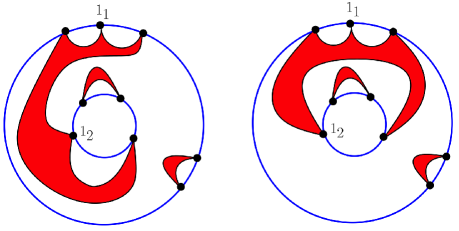
Figure 1. Two different representations of the same partition.

In this paper we study enumerative properties of this geometric representation. From this study we deduce asymptotic estimates for the subjacent non-crossing partitions for every surface $\Sigma$.

Our results and techniques.

The main result of this paper is the following: let $\Sigma$ be a surface with Euler characteristic $\chi\left(\Sigma\right)$ and whose boundary has $\beta\left(\Sigma\right)$ connected components. Then the number of non-crossing partitions on $\Sigma$, $C_{\Sigma}(n)=|\Pi_{\Sigma}(n)|$, verifies the asymptotic upper bound

(1) $$|\Pi_{\Sigma}(n)|\leq_{n\rightarrow\infty}\frac{c(\Sigma)}{\Gamma\left(-3/2\chi(\Sigma)+\beta(\Sigma)\right)}\cdot n^{-3/2\chi(\Sigma)+\beta(\Sigma)-1}\cdot 4^{n},$$

where $\Gamma$ is the Gamma function: $\Gamma(u)=\int_{0}^{\infty}t^{u-1}e^{-t}dt$. (For a bound on $c(\Sigma)$, see Section 5.) This upper bound, together with the fact that every non-crossing partition on a disk admits a realization on $\Sigma$ (in other words, $C(n)\leq C_{\Sigma}(n)$), give the result

(2) $$\lim_{n\rightarrow\infty}C_{\Sigma}(n)^{1/n}=\lim_{n\rightarrow\infty}C(n)^{1/n}=4.$$

In other words, $C_{\Sigma}(n)$ has the same exponential growth as the Catalan numbers, no matter the surface $\Sigma$.

In order to get the upper bound (1), we argue in three levels: we start from a topological level, stating the precise definitions of the objects we want to study, and showing that we can restrict ourselves to the study of hypermaps and bipartite maps [5]. Once we restrict ourselves to the map enumeration framework, we use the ideas of [2], joint with the work by Chapuy, Marcus, and Schaeffer on the enumeration of higher genus maps [4] and constellations [3] in order to obtain combinatorial decompositions of the dual maps of the objects under study. Finally, once we have explicit expressions for the generating functions of these combinatorial families, we study generating functions (formal power series) as analytic objects. In the analytic step, we extract singular expansions of the counting series from the resulting generating functions. We derive asymptotic formulas from these singular expansions by extracting coefficients, using the Transfer Theorems of singularity analysis [8, 10].

Application to algorithmic graph theory.

The asymptotic analysis carried out in this paper has important consequences in the design of algorithms for graphs on surfaces: the enumeration of non-crossing partitions has been used in [15] to build a framework for the design of $2^{O(k)}\cdot n^{O(1)}$ step dynamic programming algorithms to solve a broad class of NP-hard optimization problems for surface-embedded graphs on $n$ vertices of branchwidth at most $k$. The approach is based on a new type of branch decomposition called surface cut decomposition, which generalizes sphere cut decompositions for planar graphs introduced by Seymour and Thomas [16], and where dynamic programming should be applied for each particular problem. More precisely, the use of surface cut decompositions yields algorithms with running times with a single-exponential dependence on branchwidth, and allows to unify and improve all previous results in this active field of parameterized complexity [6, 7]. The key idea is that the size of the tables of a dynamic programming algorithm over a surface cut decomposition can be upper-bounded in terms of the non-crossing partitions on surfaces with boundary. See [15] for more details and references.

Outline of the paper.

In Section 2 we include all the definitions and the required background concerning topological surfaces, maps on surfaces, the symbolic method in combinatorics, and the singularity analysis on generating functions. In Section 3 we state the precise definition of non-crossing partition on a general surface, as well as the connection with the map enumeration framework. Upper bounds for the number of non-crossing partitions on a surface $\Sigma$ with boundary are obtained in Section 4, and the main result is proved. A more detailed study of the constant $c(\Sigma)$ of Equation (1) is done in Section 5.

2. Background and definitions

In this section we state all the necessary definitions and results needed in the sequel. In Subsection 2.1 we state the main results concerning topological surfaces, and in Subsection 2.2 we recall the basic definitions about maps on surfaces. Finally, in Subsection 2.3 we make a brief summary of the symbolic method in combinatorics, as well as the basic techniques in singularity analysis on generating functions.

2.1. Topological surfaces

In this work, surfaces are compact (hence closed and bounded) and their boundary is homeomorphic to a finite set (possibly empty) of disjoint simple circles. We denote by $\beta\left(\Sigma\right)$ the number of connected components of the boundary of a surface $\Sigma$. The Surface Classification Theorem [14] asserts that a compact and connected surface without boundary is determined, up to homeomorphism, by its Euler characteristic $\chi\left(\Sigma\right)$ and by its orientability. More precisely, orientable surfaces are obtained by adding $g\geq 0$ handles to the sphere $\mathbb{S}^{2}$, obtaining a surface with Euler characteristic $2-2g$. Non-orientable surfaces are obtained by adding $h>0$ cross-caps to the sphere, getting a non-orientable surface with Euler characteristic $2-h$. We denote by $\overline{\Sigma}$ the surface (without boundary) obtained from $\Sigma$ by gluing a disk on each of the $\beta(\Sigma)$ components of the boundary of $\Sigma$. It is then easy to show that $\chi\left(\overline{\Sigma}\right)=\beta(\Sigma)+\chi(\Sigma)$. In other words, surfaces under study are determined, up to homeomorphism, by their orientability, their Euler characteristic, and t he number of connected components of their boundary.

A cycle on $\Sigma$ is a topological subspace of $\Sigma$ which is homeomorphic to a circle. We say that a cycle $\mathbb{S}^{1}$ separates $\Sigma$ if $\Sigma\setminus\mathbb{S}^{1}$ has two connected components. The following result concerning a separating cycle is an immediate consequence of [14, Proposition 4.2.1].

Lemma 2.1.1.

Let $\Sigma$ be a surface with boundary and let $\mathbb{S}^{1}$ be a separating cycle on $\Sigma$. Let $V_{1}$ and $V_{2}$ be connected surfaces obtained by cutting $\Sigma$ along $\mathbb{S}^{1}$ and gluing a disk on the newly created boundaries. Then $\chi(\Sigma)=\chi(V_{1})+\chi(V_{2})-2$.

2.2. Maps on surfaces and duality

Our main reference for maps is the monograph of Lando and Zvonkin [13]. A map on $\Sigma$ is a partition of $\Sigma$ in zero, one, and two dimensional sets homeomorphic to zero, one and two dimensional open disks, respectively (in this order, vertices, edges, and faces). The set of vertices, edges and faces of a map $M$ is denoted by $V(M)$, $E(M)$, and $F(M)$, respectively. We use $v(M),e(M)$, and $f(M)$ to denote $|V(M)|,|E(M)|$, and $|F(M)|$, respectively. The degree $\mathbf{\mathrm{d}}(v)$ of a vertex $v$ is the number of edges incident with $v$, counted with multiplicity (loops are counted twice). An edge of a map has two ends (also called half-edges), and either one or two sides, depending on the number of faces which is incident with. A map is rooted if an edge and one of its half-edges and sides are distinguished as the root-edge, root-end, and root-side, respectively. Observe that rooting on orientable surfaces usually omits the choice of a root-side because the subjacent surface carries a global orientation, and maps are considered up to orientation-preserving homeomorphism. Our choice of a root-side is equivalent in the orientable case to the choice of an orientation of the surface. The root-end and -sides define the root-vertex and -face, respectively. Rooted maps are considered up to cell-preserving homeomorphisms preserving the root-edge, -end, and -side. In figures, the root-edge is indicated as an oriented edge pointing away from the root-end and crossed by an arrow pointing towards the root-side (this last, provides the orientation in the surface). For a map $M$, the Euler characteristic of $M$, which is denoted by $\chi(M)$, is the Euler characteristic of the underlying surface.

Duality.

Given a map $M$ on a surface $\Sigma$ without boundary, the dual map of $M$, which we denote by $M^{*}$, is a map on $\Sigma$ obtained by drawing a vertex of $M$ in each face of $M$ and an edge of $M$ across each edge of $M$. If the map $M$ is rooted, the root-edge $e$ of $M$ is defined in the natural way: the root-end and root-side of $M$ correspond to the side and end of $e$ which are not the root-side and root-end of $M$, respectively. This construction can be generalized to surfaces with boundary in the following way: for a map $M$ on a surface $\Sigma$ with boundary, notice that the (rooted) map $M$ defines a (rooted) map $\overline{M}$ on $\overline{\Sigma}$ by gluing a disk (which becomes a face of $\overline{M}$) along each boundary component of $\Sigma$. We call these faces of $\overline{M}$ external. Then the usual construction for the dual map $\overline{M}^{*}$ applies using the external faces. The dual of a map $M$ on a surface $\Sigma$ with boundary is the map on $\overline{\Sigma}$, denoted $M^{*}$, constructed from $\overline{M}^{*}$ by splitting each external vertex of $\overline{M}^{*}$. The new vertices that are obtained are called dangling leaves, which have degree one. Observe that we can reconstruct the map $M$ from $M^{*}$, by pasting the dangling leaves incident with the same face, and applying duality. An example of this construction is shown in Figure 2.

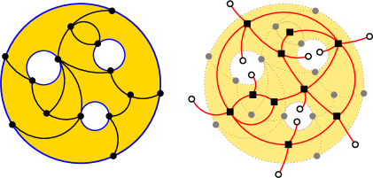
Figure 2. A map with boundary and its dual.

2.3. The symbolic method and analytic combinatorics

Our main reference in enumerative combinatorics is the book of Flajolet and Sedgewick [8]. The framework introduced in this book gives a language to translate combinatorial conditions between combinatorial classes into equations relating the associated generating functions. This is what is called the symbolic method in combinatorics. Later, we can treat these equations as relations between analytic functions. This point of view gives the possibility to use complex analysis techniques to obtain information about the combinatorial classes. This is the origin of the term analytic combinatorics.

The symbolic method.

For a set $\mathcal{A}$ of objects, let $|\cdot|$ be an application (called size) from $\mathcal{A}$ to $\mathbb{N}$. We assume that the number of elements in $\mathcal{A}$ with a fixed size is always finite. A pair $(\mathcal{A},|\cdot|)$ is called a combinatorial class. Under these assumptions, we define the formal power series (called the generating function or GF associated with the class) $\textbf{A}(x)=\sum_{a\in\mathcal{A}}x^{|a|}=\sum_{n=0}^{\infty}a_{n}x^{n}$. Conversely, we write $a_{n}=[x^{n}]\textbf{A}(x)$. The symbolic method provides a direct way to translate combinatorial constructions between combinatorial classes into equations between GFs. The constructions we use in this work and their translation into the language of GFs are shown in Table 1.

Construction		GF
Union	$\mathcal{A}\cup\mathcal{B}$	$\textbf{A}(x)+\textbf{B}(x)$
Product	$\mathcal{A}\times\mathcal{B}$	$\textbf{A}(x)\textbf{B}(x)$
Sequence	$\mathrm{Seq}\left(\mathcal{A}\right)$	$\frac{1}{1-\textbf{A}(x)}$
Pointing	$\mathcal{A}^{\bullet}$	$x\frac{\partial}{\partial x}\textbf{A}(x)$

Table 1. Constructions and translations into GFs.

The union $\mathcal{A}\cup\mathcal{B}$ of $\mathcal{A}$ and $\mathcal{B}$ refers to the disjoint union of the classes. The cartesian product $\textrm{A}\times\mathcal{B}$ of $\mathcal{A}$ and $\mathcal{B}$ is the set $\{(a,b):a\in\mathcal{A},\,b\in\mathcal{B}\}$. The sequence $\mathrm{Seq}\left(\mathcal{A}\right)$ of a set $\mathcal{A}$ corresponds to the set $\mathcal{E}\cup\mathcal{A}\cup\left(\mathcal{A}\times\mathcal{A}\right)\cup\left(\mathcal{A}\times\mathcal{A}\times\mathcal{A}\right)\cup\ldots$, where $\mathcal{E}$ denotes the empty set. At last, the pointing operator $\mathcal{A}^{\bullet}$ of a set $\mathcal{A}$ consists in pointing one of the atoms of each element $a\in\mathcal{A}$. Notice that in the sequence construction, the expression $\mathcal{E}\cup\mathcal{A}\cup\left(\mathcal{A}\times\mathcal{A}\right)\cup\left(\mathcal{A}\times\mathcal{A}\times\mathcal{A}\right)\cup\dots$ translates into $\sum_{k=0}^{\infty}\textbf{A}(x)^{k}$, which is a sum of a geometric series. In the case of pointing, note also that $x\frac{\partial}{\partial z}\textbf{A}(x)=\sum_{n>0}na_{n}x^{n}$.

Singularity analysis.

The study of the asymptotic growth of the coefficients of GFs can be obtained by considering GFs as complex functions analytic around $z=0$. This is the main idea of analytic combinatorics. The growth behavior of the coefficients depends only on the smallest positive singularity of the GF. Its location provides the exponential growth of the coefficients, and its behavior gives the subexponential growth of the coefficients.

More concretely, for real numbers $R>\rho>0$ and $0<\phi<\pi/2$, let $\Delta_{\rho}(\phi,R)$ be the set $\{z\in\mathbb{C}:|z|<R,\,z\neq\rho,\,|\mathrm{Arg}(z-\rho)|>\phi\}$. We call a set of this type a dented domain or a domain dented at $\rho$. Let $\textbf{A}(z)$ and $\textbf{B}(z)$ be GFs whose smallest singularity is the real number $\rho$. We write $\textbf{A}(z)\sim_{z\rightarrow\rho}\textbf{B}(z)$ if $\lim_{z\rightarrow\rho}\textbf{A}(z)/\textbf{B}(z)=1$. We obtain the asymptotic expansion of $[z^{n}]\textbf{A}(z)$ by transfering the behavior of $\textbf{A}(z)$ around its singularity from a simpler function $\textbf{B}(z)$, from which we know the asymptotic behavior of their coefficients. This is the main idea of the so-called Transfer Theorems developed by Flajolet and Odlyzko [10]. These results allows us to deduce asymptotic estimates of an analytic function using its asymptotic expansion near its dominant singularity. In our work we use a mixture of Theorems VI.1 and VI.3 from [8]:

Proposition 2.3.1 (Transfer Theorem).

If $\textbf{A}(z)$ is analytic in a dented domain $\Delta=\Delta_{\rho}(\phi,R)$, where $\rho$ is the smallest singularity of $\textbf{A}(z)$, and

$$\textbf{A}(z)\underset{z\in\Delta,z\rightarrow\rho}{\sim}c\cdot\left(1-\frac{z}{\rho}\right)^{-\alpha}+O\left(\left(1-\frac{z}{\rho}\right)^{-\alpha+\gamma}\right),$$

for $\alpha\not\in\{0,-1,-2,\ldots\}$, and $\gamma>0$ then

(3) $$a_{n}\ =c\cdot\frac{n^{\alpha-1}}{\Gamma(\alpha)}\cdot\rho^{-n}\left(1+O(n^{-\gamma})\right),$$

where $\Gamma$ is the Gamma function: $\Gamma(u)=\int_{0}^{\infty}t^{u-1}e^{-t}dt$.

3. Non-crossing partitions on surfaces with boundary

In this section we introduce the precise definition of a non-crossing partition on a surface with boundary. The notion of a non-crossing partition on a general surface is not as simple as in the case of a disk, and must be stated in terms of objects more general than maps. Our strategy to obtain asymptotic estimates for the number of non-crossing partitions on surfaces consists in showing that we can restrict ourselves to the study of certain families of maps. More concretely, we show that the study of non-crossing partitions is a particular case of the study of hypermaps [5], which can be interpreted as bipartite maps. The plan for this section is the following: in Subsection 3.1 we set up our notation and we define a non-crossing partition on a general surface. In Subsection 3.2 we show that we can restrict ourselves to the study of bipartite maps in which vertices belong to the boundary of the surface.

3.1. Bipartite subdivisions and non-crossing partitions

Let $\Sigma$ be a connected surface with boundary, and let $\mathbb{S}^{1}_{1},\mathbb{S}^{1}_{2},\dots,\mathbb{S}^{1}_{\beta(\Sigma)}$ be the connected components of the boundary of $\Sigma$.

A bipartite subdivision $S$ of $\Sigma$ with $n$ vertices is a decomposition of $\Sigma$ into zero-, one-, and two-dimensional open and connected subsets, where the $n$ vertices lay on the boundary of $\Sigma$, and there is a two-coloring (namely, using black and white colors) of the two-dimensional regions, such that each vertex is incident (possibly more than once) with a unique black two-dimensional region. We use the notation $A(S)$ to denote the set $A_{1}\cup\cdots\cup A_{\beta(\Sigma)}$ of vertices of $S$.

Figure 3. Geometric representation of non-crossing partitions on a disk, on a cylinder, and on a Möbius band.

For $1\leq r\leq\beta(\Sigma)$, let $A_{r}=\{1_{\{r\}},2_{\{r\}},\dots,n_{\{r\}}\}$ be the set of vertices on $\mathbb{S}^{1}_{r}$, i.e., $A_{r}=A(S)\cap\mathbb{S}^{1}_{r}$. Vertices on each boundary are labeled in counterclockwise order, and satisfy the property that $|A_{1}|+|A_{2}|+\dots+|A_{\beta(\Sigma)}|=n$. In particular, boundary components are distinguishable. Observe that an equivalent way to label these vertices is distinguishing on each boundary component an edge-root, whose ends are vertices $1_{\{r\}}$ and $2_{\{r\}}$.

In general, bipartite subdivisions are not maps: two-dimensional subsets could not be homeomorphic to open disks. Black faces on a bipartite subdivision are called blocks. A block of size $k$ is regular if it is incident with exactly $k$ vertices and it is contractible (i.e., homeomorphically equivalent to a disk). A bipartite subdivision is regular if each block is regular. All bipartite subdivisions are rooted: every connected component of the boundary of $\Sigma$ is edge-rooted in counterclockwise order. We denote by $\mathcal{S}_{\Sigma}(n)$ and $\mathcal{R}_{\Sigma}(n)$ the set of general and regular bipartite subdivisions of $\Sigma$ with $n$ vertices, respectively. Observe that the total number of vertices is distributed among all the components of the boundary of $\Sigma$. In particular, it is possible that a boundary component is not incident with any vertex. See Figure 4 for examples of bipartite subdivisions. In particular, the darker blocks in the first bipartite subdivision are not regular.

Figure 4. Three bipartite subdivisions $S_{1},S_{2}$ and $S_{3}$. $S_{2}$ is regular but not reducible while $S_{3}$ is irreducible.

Let $S$ be a bipartite subdivision $S$ of $\Sigma$ with $n$ vertices and let $X_{1},\ldots,X_{r}$ the set ${\mathcal{S}}$ be its blocks. Clearly, these blocks define the partition $\pi_{\Sigma}\left(S\right)=\{X_{1}\cap A,\ldots,X_{r}\cap A\}$ of the vertex set $A=A_{1}\cup\dots\cup A_{\beta(\Sigma)}$. We say that a partition of $A$ is non-crossing if it is equal to $\pi_{\Sigma}\left(S\right)$ for some bipartite subdivision $S$ of $\Sigma$. A non-crossing partition is said to be regular if it arises from a regular bipartite subdivision. Observe that this definition generalizes the notion of a non-crossing partition on a disk. We define $\Pi_{\Sigma}(n)$ as the set of non-crossing partitions of $\Sigma$ with $n$ vertices and we set $C_{\Sigma}=|\Pi_{\Sigma}(n)|$. Notice that this definition of $\Pi_{\Sigma}$ is equivalent to the one we gave in the introduction. In the rest of the paper we adopt the new definition as this will simplify the presentation of our results and proofs.

3.2. Reduction to the map framework

In this subsection we show that we can restrict ourselves to the study of bipartite maps in which vertices belong to the boundary of the surface. Later, this reduction will allow to study non-crossing partitions in the context of map enumeration.

Let $\Sigma_{1}$ and $\Sigma_{2}$ be surfaces with boundary. We write $\Sigma_{2}\subset\Sigma_{1}$ if there exists a continuous injection $i:\Sigma_{2}\hookrightarrow\Sigma_{1}$ such that $i(\Sigma_{2})$ is homeomorphic to $\Sigma_{2}$. If $S$ is a bipartite subdivision of $\Sigma_{2}$ and $\Sigma_{2}\subset\Sigma_{1}$, then the injection $i$ induces a bipartite subdivision $i(S)$ on $\Sigma_{1}$ such that $\pi_{\Sigma_{2}}(S)=\pi_{\Sigma_{1}}\left(i(S)\right)$. Roughly speaking, all bipartite subdivisions on $\Sigma_{2}$ can be realized on a surface $\Sigma_{1}$ which contains $\Sigma_{2}$. One can write then that $\Pi_{\Sigma_{2}}(n)\subseteq\Pi_{\Sigma_{1}}(n)$ if $\Sigma_{2}\subset\Sigma_{1}$, and then it holds that $|\Pi_{\Sigma_{2}}(n)|\leq|\Pi_{\Sigma_{1}}(n)|$. This proves the trivial bound $C(n)\leq|\Pi_{\Sigma}(n)|$ for all choices of $\Sigma$.

As the following lemma shows, regularity is conserved by injections of surfaces.

Lemma 3.2.1.

Let $M_{1}$ be a regular bipartite subdivision of $\Sigma_{1}$, and let $\Sigma_{1}\subset\Sigma$. Then $M_{1}$ defines a regular bipartite subdivision $M$ over $\Sigma$ such that $\pi_{\Sigma_{1}}\left(M_{1}\right)=\pi_{\Sigma}(M)$.

Proof.

Let $i:\Sigma_{1}\hookrightarrow\Sigma$ be the corresponding injective application, and consider $M=i\left(M_{1}\right)$. In particular, a block $\pi$ of $M_{1}$ is topologically equivalent to the block $i(\pi)$: $i$ is a homeomorphism between $\Sigma$ and $i(\Sigma)$. Hence $i(\pi)$ is an open contractible set and $M$ is regular. ∎

The following proposition allows us to reduce the problem to the study of regular bipartite subdivisions.

Lemma 3.2.2.

Let $S\in\mathcal{S}_{\Sigma}(n)$ be a bipartite subdivision of $\Sigma$ and let $\pi_{\Sigma}(S)$ be the associated non-crossing partition on $\Sigma$. Then, there exists a regular bipartite subdivision $R\in\mathcal{R}_{\Sigma}(n)$ such that $\pi_{\Sigma}(R)=\pi_{\Sigma}(S)$.

Proof.

Each bipartite subdivision has a finite number of blocks. For each block we will apply a finite number of transforms in order to change it into a regular block, without changing the associated non-crossing partition. We consider two cases according to whether the block studied is contractible or not.

Let $f$ be a contractible block of $S$. Suppose that the boundary of $f$ consists of more than one connected component. We define the operation of joining boundaries as follows: let $l$ be a path that joins a vertex $v$ in one component of the boundary of $f$ with a vertex $u$ in another component of the boundary. This path exists because $f$ is a connected and open subset of $\Sigma$. Consider also two paths $l_{1},l_{2}$ that join these two vertices around the initial path $l$, as illustrated in Figure 5. Note that these paths $l_{1}$ and $l_{2}$ also exist since we are dealing with open subsets. We define the new block $f_{1}$ as the one obtained from the initial block $f$ by deleting the face defined by $l_{1}$ and $l_{2}$ which contains $l$ (see the leftmost part of Figure 5 for an example). Let $s_{1}$ be the resulting bipartite subdivision. Observe that the number of connected components of the boundary of $f_{1}$ is the same as for $f$ minus one. We can apply this argument over $f$ as many times as the number of components of the boundary of $f$ is strictly greater than one. At the end, we obtain a bipartite subdivision with the same induced non-crossing partition, such that the block derived from $f$ has exactly one boundary component.

Suppose now that the boundary of the block $f$ has a single component, but it is not simple. Let $v$ be a vertex incident $p>1$ times with $f$. In this case we define the operation of cutting a vertex as follows: consider the intersection of a small ball of radius $\epsilon>0$ centered at $v$ with the block $f$, namely $B_{\epsilon}(v)\cap f$. Observe that $\left(B_{\epsilon}(v)\cap f\right)\backslash\{v\}$ has exactly $p$ connected components. We define the new block by deforming $p-1$ of these components in such a way that they do not intersect the boundary of $\Sigma$. Next, we paste the vertex $v$ to the unique component which has not been deformed (see the rightmost part of Figure 5 for an example). Then the resulting bipartite subdivision has the same associated non-crossing partition, and $v$ is incident with the corresponding block exactly once. Applying this argument for each vertex of $f$ we get a block with a single simple boundary.

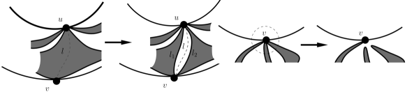
Figure 5. The operations of joining boundaries and cutting vertices.

Summarizing, from each contractible block $f$ of $S$ we construct a new block $f^{\prime}$ which is incident with the same vertices as $f$.

To conclude, suppose now that $f$ is an non-contractible block of $S$. Let $\mathbb{S}^{1}_{f}$ be a non-contractible cycle contained in $f$. We cut the surface along this cycle. We paste either a disk or a pair of disks along the border depending on whether $\mathbb{S}^{1}_{f}$ is one- or two-sided. This operation either increases the number of connected components or decreases the genus of the surface.

Observe that the number of times we need to apply this operation is bounded by $-\chi(\Sigma)$; in particular, it is finite. At the end, after converting each block to a contractible one, all blocks are contractible and the resulting surface (possibly with many connected components) is $\Sigma_{1}\subset\Sigma$. The resulting bipartite subdivision $M^{\prime}$ on $\Sigma_{1}$ is regular (since all the blocks are regular), and then by Lemma 3.2.1 there exists a regular bipartite subdivision $R$ over $\Sigma$ such that $\pi_{\Sigma}\left(R\right)=\pi_{\Sigma_{1}}\left(M^{\prime}\right)$, as claimed. ∎

Notice that we just proved the following.

(4) $$|\Pi_{\Sigma}(n)|\leq|\mathcal{R}_{\Sigma}(n)|.$$

We say that a bipartite subdivision $M$ is irreducible in $\Sigma_{1}$ if the associated non-crossing partition $\pi_{\Sigma_{1}}(M)$ is regular and all its white faces are contractible. In this case, we also say that the non-crossing partition $\pi_{\Sigma_{1}}(M)$ is irreducible. We denote by $\mathcal{P}_{\Sigma}(n)$ the set of irreducible bipartite subdivisions. Clearly, the following holds.

(5) $$|\mathcal{P}_{\Sigma}(n)|\leq|\mathcal{R}_{\Sigma}(n)|.$$

The following lemma is a basic consequence of the previous discussions, and allows us to reduce our study to the enumeration in the context of maps.

Lemma 3.2.3.

Let $M$ be an irreducible bipartite subdivision of $\Sigma$. Then the two-dimensional regions of $M$ are all contractible (hence, faces).

Proof.

From Lemma 3.2.2, we only need to deal with white two-dimensional regions. For a white face whose interior is not homeomorphic to an open disk, there exists a non-contractible cycle $\mathbb{S}^{1}$. Cutting along $\mathbb{S}^{1}$ we obtain a surface $\Sigma^{\prime}$ such that $\Sigma^{\prime}\subset\Sigma$ and $M$ is induced in $\Sigma^{\prime}$, a contradiction. As a conclusion, all faces are contractible. ∎

The above lemma says that irreducible bipartite subdivisions define bipartite maps. In the next section we reduce our study to the family of irreducible bipartite subdivisions. This permits us to upper-bound $|\mathcal{P}_{\Sigma}(n)|$ instead of dealing with the more complicated task of upper-bounding $|\mathcal{R}_{\Sigma}(n)|$. The reason why this also gives an asymptotic bound for $|\Pi_{\Sigma}(n)|$ is that the subfamily $\mathcal{P}_{\Sigma}(n)$ provides the main contribution to the asymptotic estimates for $\mathcal{R}_{\Sigma}(n)$. Therefore (5) can be seen, asymptotically, as an equality, and, that way, the result follows from (4).

4. Upper bounds for non-crossing partitions on surfaces

The plan for this section is the following: in Subsection 4.1 we introduce families of plane trees that arise by duality on non-crossing partitions on a disk. These combinatorial structures are used in Subsection 4.2 to obtain a tree-like structure which provides a way to obtain asymptotic estimates for the number of irreducible bipartite subdivisions of $\Sigma$ with $n$ vertices, $|\mathcal{P}_{\Sigma}(n)|$. These asymptotic estimates are found in Subsection 4.3 for irreducible bipartite subdivisions. Finally, we prove in Subsection 4.4 that the number of irreducible bipartite subdivisions is asymptotically equal to the number of bipartite subdivisions, hence the estimate obtained in Subsection 4.2 is an upper bound for the number of non-crossing partitions on surfaces. All previous steps are summarized in Subsection 4.5.

4.1. Planar constructions

The dual map of a non-crossing partition on a disk is a tree, which is called the (non-crossing partition) tree associated with the non-crossing partition. This tree corresponds to the notion of dual map for surfaces with boundary introduced in Subsection 2.2. Recall that vertices of degree one are called the dangling leaves of the tree. Vertices of the tree are called block vertices if they are associated with a block of the non-crossing partition. The remaining vertices are either non-block vertices or danglings. By construction, all vertices adjacent to a block vertex are non-block vertices. Conversely, each vertex adjacent to a non-block vertex is either a block vertex or a dangling. Graphically, we use the symbols $\blacksquare$ for block vertices, $\square$ for non-block vertices and $\circ$ for danglings. Non-crossing partitions trees are rooted: the root of a non-crossing partition tree is defined by the root of the initial non-crossing partition on a disk. The block vertex which carries the role of the root vertex of the tree is the one associated with the block containing vertex with label $2$ (or equivalently, the end-vertex of the root). See Figure 6 for an example of this construction.

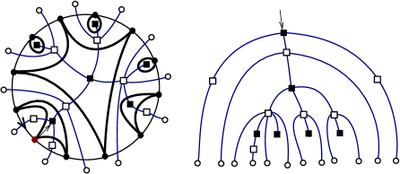
Figure 6. A non-crossing partition on a disk and the associated non-crossing partition tree.

Let $\mathcal{T}$ be the set of non-crossing partitions trees, and let $\mathbf{T}=\mathbf{T}(z,u)=\sum_{n,m\geq 0}t_{n,m}z^{n}u^{m}$ be the corresponding generating function. The variable $z$ marks danglings and $u$ marks block vertices. We use an auxiliary family $\mathcal{B}$, defined as the set of trees which are rooted at a non-block vertex. Let $\mathbf{B}=\mathbf{B}(z,u)=\sum_{n,m\geq 0}b_{n,m}z^{n}u^{m}$ be the associated generating function. The next lemma gives the exact enumeration of $\mathcal{T}$ and $\mathcal{B}$. In particular, this lemma implies the well-known Catalan numbers for non-crossing partitions on a disk.

Lemma 4.1.1.

The number of non-crossing trees counted by the number of danglings and block vertices is enumerated by the generating function

(6) $$\mathbf{T}(z,u)=\frac{1-z(1-u)-\sqrt{(z(1-u)-1)^{2}-4zu}}{2zu}.$$

Furthermore, $\mathbf{B}(z,u)=z\mathbf{T}(z,u)$.

Proof.

We establish combinatorial relations between $\mathcal{B}$ and $\mathcal{T}$ from which we deduce the result. Observe that there is no restriction on the number of vertices incident with a given block. Hence the degree of every block vertex is arbitrary. This condition is translated symbolically via the relation

$$\mathcal{T}=\{\blacksquare\}\times\mathrm{Seq}\left(\mathcal{B}\right).$$

Similarly, $\mathcal{B}$ can be written in the form

$$\mathcal{B}=\{\circ\}\times\mathrm{Seq}\left(\mathcal{T}\times\{\circ\}\right).$$

These combinatorial conditions translate using Table 1 into the system of equations

$$\mathbf{T}=\frac{u}{1-\mathbf{B}},\ ,\ \ \mathbf{B}=\frac{z}{1-z\mathbf{T}}.$$

Substituting the expression of $\mathbf{B}$ in the first equation, one obtains that $\mathbf{T}$ satisfies the relation $z\mathbf{T}^{2}+(z(1-u)-1)\mathbf{T}+u=0$. The solution to this equation with positive coefficients is (6). Solving the previous system of equations in terms of $\mathbf{B}$ brings $\mathbf{B}=z\mathbf{T}$, as claimed. ∎

Observe that writing $u=1$ in $\mathbf{T}$ and $\mathbf{B}$ we obtain that $\mathbf{T}(z)=\mathbf{T}(z,1)=\frac{1-\sqrt{1-4z}}{2z}$, and $\mathbf{B}(z)=\mathbf{B}(z,1)=z\mathbf{T}(z)$, deducing the well-known generating function for Catalan numbers.

We introduce another family of trees related to non-crossing partitions trees, which we call double trees. A double tree is defined in the following way: consider a path where we concatenate block vertices and non-block vertices. We consider the internal vertices of the path. A double tree is obtained by pasting on every block vertex of the path a pair of elements of $\mathcal{T}$ (one at each side of the path), and a pair of elements of $\mathcal{B}$ for non-block vertices. We say that a double tree is of type either $\blacksquare-\blacksquare$, $\blacksquare-\square$, or $\square-\square$ depending on the ends of the path. An example for a double tree of type $\blacksquare-\blacksquare$ is shown in Figure 7.

Figure 7. A double tree and its decomposition.

We denote these families by $\mathcal{T}_{\blacksquare-\blacksquare}$, $\mathcal{T}_{\square-\blacksquare}$, and $\mathcal{T}_{\square-\square}$, and the corresponding generating function by $\mathbf{T}_{1}(z,u)=\mathbf{T}_{1}$, $\mathbf{T}_{2}(z,u)=\mathbf{T}_{2}$, and $\mathbf{T}_{3}(z,u)=\mathbf{T}_{3}$, respectively. Recall that in all cases $z$ marks danglings and $u$ marks block vertices. A direct application of the symbolic method provides a way to obtain explicit expressions for the previously defined generating functions. The decomposition and the GFs of the three families are summarized in Table 2.

Family	Specification	Development	Compact expression
$\mathcal{T}_{\square-\blacksquare}$	$\mathrm{Seq}\left(\mathcal{B}^{2}\times\mathcal{T}^{2}\right)$	$1+\frac{1}{u}\mathbf{B}^{2}\mathbf{T}^{2}+\frac{1}{u^{2}}\mathbf{B}^{4}\mathbf{T}^{4}+\dots$	$1/(1-\mathbf{T}^{2}\mathbf{B}^{2}/u)$
$\mathcal{T}_{\blacksquare-\blacksquare}$	$\mathcal{B}^{2}\times\mathrm{Seq}\left(\mathcal{B}^{2}\times\mathcal{T}^{2}\right)$	$\mathbf{B}^{2}+\frac{1}{u}\mathbf{B}^{4}\mathbf{T}^{2}+\frac{1}{u^{2}}\mathbf{B}^{6}\mathbf{T}^{4}+\dots$	$\mathbf{B}^{2}/(1-\mathbf{T}^{2}\mathbf{B}^{2}/u)$
$\mathcal{T}_{\square-\square}$	$\mathcal{T}^{2}\times\mathrm{Seq}\left(\mathcal{B}^{2}\times\mathcal{T}^{2}\right)$	$\frac{1}{u}\mathbf{T}^{2}+\frac{1}{u^{2}}\mathbf{B}^{2}\mathbf{T}^{4}+\frac{1}{u^{3}}\mathbf{B}^{4}\mathbf{T}^{6}+\dots$	$\frac{1}{u}\mathbf{T}^{2}/(1-\mathbf{T}^{2}\mathbf{B}^{2}/u)$

Table 2. GFs for double trees.

To conclude, the family of pointed non-crossing trees $\mathcal{T}^{\bullet}$ is built by pointing a dangling on each non-crossing partition tree. In this case, the associated GF is $\mathbf{T}^{\bullet}=z\frac{\partial}{\partial z}\mathbf{T}$. Similar definitions can be done for the family $\mathcal{B}$. Pointing a dangling defines a unique path between this distinguished dangling and the root of the tree.

4.2. The scheme of an irreducible bipartite subdivision.

In this subsection we generalize the construction of non-crossing partition trees introduced in Subsection 4.1. In order to characterize it, we exploit the dual construction for maps on surfaces (see Subsection 2.2). More concretely, for an element $M\in\mathcal{P}_{\Sigma}(n)$, let $M^{*}$ be the dual map of $M$ on $\overline{\Sigma}$. By construction, there is no incidence in $M^{*}$ between either pairs of block vertices or pairs of non-block vertices.

From $M^{*}$ we define a new rooted map (a root for each boundary component of $\Sigma$) on $\overline{\Sigma}$ in the following way: we start by deleting recursively vertices of degree one which are not roots. Then we continue dissolving vertices of degree two, that is, replacing the two edges incident to a vertex of degree two with a single edge. The resulting map has $\beta(\Sigma)$ faces and all vertices have degree at least three (apart from root vertices, which have degree one), and vertices of two colors (vertices of different colors could be end-vertices of the same edge). The resulting map is called the scheme associated with $M$; we denote it by $\mathfrak{s}_{M}$. See Figure 8 for an example of this construction.

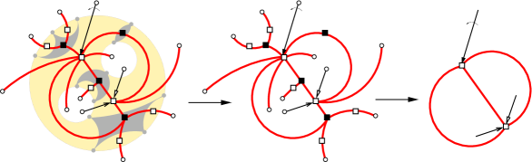
Figure 8. The construction of the scheme of an element in $\mathcal{P}_{\Sigma}$. We consider the dual of an irreducible bipartite subdivision (leftmost figure). After deleting vertices of degree one recursively and dissolving vertices of degree two, we obtain the associated scheme (rightmost figure).

The previous decomposition can be constructed in the reverse way: duals of irreducible bipartite subdivision are constructed from a generic scheme $\mathfrak{s}$ in the following way.

1. For an edge of $\mathfrak{s}$ with both end-vertices of type $\blacksquare$, we paste a double tree of type $\blacksquare-\blacksquare$ along it. Similar operations are done for edges with end-vertices $\{\square,\blacksquare\}$ and $\{\square,\square\}$.

2. For vertex $v$ of $\mathfrak{s}$ of type $\blacksquare$ we paste $\mathbf{\mathrm{d}}(v)$ elements of $\mathcal{T}$ (identifying the roots of the trees with $v$), one on each corner of $v$. The same operation is done for vertices of $\mathfrak{s}$ of type $\square$.

3. We paste an element of $\mathcal{T}^{\bullet}$ along each one of the roots of $\mathfrak{s}$ (the marked leaf determines the dangling root).

To conclude, this construction provides a way to characterize the set of schemes. Indeed, if we denote by $\mathfrak{S}_{\Sigma}$ the set of maps on $\overline{\Sigma}$ with $\beta(\Sigma)$ faces with a root on each face and with vertices of two different colors (namely, vertices of type $\blacksquare$ and $\square$), then $|\mathfrak{S}_{\Sigma}|$ is finite, since the number of faces of each element in $\mathfrak{S}_{\Sigma}$ is equal to $\beta(\Sigma)$. In fact, $\mathfrak{S}_{\Sigma}$ is the set of all possible schemes: from an arbitrary element $\mathfrak{s}\in\mathfrak{S}_{\Sigma}$ we can construct a map on $\overline{\Sigma}$ with $\beta\left(\Sigma\right)$ faces by pasting double trees along each edge of $\mathfrak{s}$ (according to the end-vertices of each edge). In other words, given $M\in\mathcal{P}_{\Sigma}(n)$ and $\mathfrak{s}_{M}$, $M^{*}$ can be reconstructed by pasting on every edge of $\mathfrak{s}_{M}$ a double tree, depending on the nature of the end-vertices of each edge of $\mathfrak{s}_{M}$. See Figure 9 for an example.

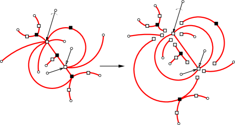
Figure 9. The decomposition into bicolored trees and the associated scheme.

4.3. Asymptotic enumeration

The decomposition introduced in Subsection 4.2 can be exploited in order to get asymptotic estimates for $|\mathcal{P}_{\Sigma}(n)|$, and consequently upper bounds for $|\Pi_{\Sigma}(n)|$. In this subsection we provide estimates for the number of irreducible bipartite subdivisions. We obtain these estimates directly for the surface $\Sigma$, while the usual technique consists in reducing the enumeration to surfaces of smaller genus, and returning back to the initial one by topological “pasting” arguments. The main point consists in exploiting tree structures of the dual graph associated with an irreducible bipartite subdivision. The main ideas are inspired by [2], where the authors find the asymptotic enumeration of simplicial decompositions of surfaces with boundaries without interior points.

We use the notation and definitions introduced in Subsection 4.1 (i.e., families of trees, double trees and pointed trees, and the corresponding GFs), joint with the decomposition introduced in Subsection 4.2. Let us now introduce some extra notation.

We denote by $\mathcal{P}_{\Sigma}(n,m)$ the set of irreducible bipartite subdivisions of $\Sigma$ with $n$ vertices and $m$ blocks. We write $p_{n,m}^{\Sigma}$ for the cardinality of this set and $\textbf{P}_{\Sigma}(z,u)=\sum_{n,m\geq 0}p_{n,m}^{\Sigma}z^{n}u^{m}$. Let $p_{n}^{\Sigma}=\sum_{m\geq 0}p_{n,m}^{\Sigma}=[z^{n}]\textbf{P}_{\Sigma}(z,1)$. Let $\mathfrak{s}\in\mathfrak{S}_{\Sigma}$. Denote by $v_{1}(\mathfrak{s})$ and $v_{2}(\mathfrak{s})$ the set of vertices of type $\blacksquare$ and $\square$ of $\mathfrak{s}$, respectively. Write $b(\mathfrak{s}),w(\mathfrak{s})$ for the number of roots which are incident with a vertex of type $\blacksquare$ and $\square$, respectively. In particular, $b(\mathfrak{s})+w(\mathfrak{s})=\beta(\Sigma)$. Denote by $e_{1}(\mathfrak{s})$ the number of edges in $\mathfrak{s}$ of type $\blacksquare-\blacksquare$. We similarly define $e_{2}(\mathfrak{s})$ and $e_{3}(\mathfrak{s})$ for edges of type $\square-\blacksquare$ and $\square-\square$, respectively. Observe that $e_{1}(\mathfrak{s})+e_{2}(\mathfrak{s})+e_{3}(\mathfrak{s})+b(\mathfrak{s})+w(\mathfrak{s})$ is equal to the number of edges of $\mathfrak{s}$, $e(\mathfrak{s})$. For a vertex $v$ of $\mathfrak{s}$, denote by $r(\mathfrak{s})$ the number of roots which are incident with it. Finally, denote by $\mathfrak{C}_{\Sigma}\subset\mathfrak{S}_{\Sigma}$ the set of maps on $\mathfrak{S}_{\Sigma}$ whose vertex degree is equal to three (namely, cubic maps on $\overline{\Sigma}$ with $\beta(\Sigma)$ faces).

The decomposition discussed in Subsection 4.2 together with Proposition 2.3.1 give the following:

Lemma 4.3.1.

Let $\Sigma$ be a surface with boundary. Then

(7) $$[z^{n}]\mathbf{P}_{\Sigma}(z,1)=p_{n}^{\Sigma}=\frac{c(\Sigma)}{\Gamma\left(-3\chi(\Sigma)/2+\beta(\Sigma\right))}\cdot n^{-3\chi(\Sigma)/2+\beta(\Sigma)-1}\cdot 4^{n}\left(1+O\left(n^{-1/2}\right)\right),$$

where $c(\Sigma)$ is a function depending only on $\Sigma$.

Proof.

According to the decomposition introduced in Subsection 4.2, $\mathbf{P}_{\Sigma}(z,u)$ can be written in the following form: for each $\mathfrak{s}\in\mathfrak{S}_{\Sigma}$, we replace edges (not roots) with double trees, roots with pointed trees, and vertices with sets of trees. More concretely,

$$\textbf{P}_{\Sigma}(z,u)=\sum_{\mathfrak{s}\in\mathfrak{S}_{\Sigma}} u^{\left|v_{1}(\mathfrak{s})\right|}\mathbf{T}_{1}^{e_{1}(\mathfrak{s})}\mathbf{T}_{2}^{e_{2}(\mathfrak{s})}\mathbf{T}_{3}^{e_{3}(\mathfrak{s})}\left(\frac{\mathbf{T}}{u}\right)^{\sum_{x\in v_{1}(\mathfrak{s})}(\mathbf{\mathrm{d}}(x)-2r(x))}\times$$

$$\mathbf{B}^{\sum_{y\in v_{2}(\mathfrak{s})}(\mathbf{\mathrm{d}}(y)-2r(y))}\left(\frac{\mathbf{T}^{\bullet}}{u}\right)^{B(\mathfrak{s})}\left(\mathbf{B}^{\bullet}\right)^{W(\mathfrak{s})}.$$

Observe in the previous expression that terms $\mathbf{T}$ and $\mathbf{T}^{\bullet}$ appear divided by $u$: blocks on the dual map are considered in the term $u^{\left|v_{1}(\mathfrak{s})\right|}$, so we do not consider the root of the different non-crossing trees.

To obtain the asymptotic behavior in terms of the number of danglings, we write $u=1$ in Equation (4.3). To study the resulting GF, we need the expression of each factor of Equation (4.3) when we write $u=1$; all these expressions are shown in Table 3. This table is built from the expressions for $\mathbf{T}$ and $\mathbf{B}$ deduced in Lemma 4.1.1 and the expressions for double trees in Table 2.

GF	Expression
$\mathbf{T}_{1}(z,1)$	$1/16(1-4z)^{-1/2}-1/8(1-4z)^{1/2}+1/16(1-4z)^{3/2}$
$\mathbf{T}_{2}(z,1)$	$1/4(1-4z)^{-1/2}+1/2+(1-4z)^{1/2}$
$\mathbf{T}_{3}(z,1)$	$z^{2}\left(1/16(1-4z)^{-1/2}-1/8(1-4z)^{1/2}+1/16(1-4z)^{3/2}\right)$
$\mathbf{T}(z,1)$	$(1-(1-4z)^{1/2})/(2z)$
$\mathbf{B}(z,1)$	$\left(1-(1-4z)^{1/2}\right)/2$
$\mathbf{T}^{\bullet}(z,1)$	$(1-4z)^{-1/2}/z-(1-(1-4z)^{-1/2})/(2z^{2})$
$\mathbf{B}^{\bullet}(z,1)$	$(1-4z)^{-1/2}$

Table 3. Univariate GF for all families of trees.

The GF in Equation (4.3) is a finite sum (a total of $|\mathfrak{S}_{\Sigma}|$ terms), so its singularity is located at $z=1/4$ (since each addend has a singularity at this point). For each choice of $\mathfrak{s}$,

(9) $$\mathbf{T}(z,1)^{\sum_{x\in v_{1}(\mathfrak{s})}(\mathbf{\mathrm{d}}(x)-2r(x))}\mathbf{B}(z,1)^{\sum_{y\in v_{2}(\mathfrak{s})}(\mathbf{\mathrm{d}}(y)-2r(y))}=\sum_{n=0}^{f(\mathfrak{s})}f_{n}(z)(1-4z)^{n/2},$$

where the positive integer $f(\mathfrak{s})$ depends only on $\mathfrak{s}$, $f_{n}(z)$ are functions analytic at $z=1/4$, and $f_{0}(z)\neq 0$ at $z=1/4$. For the other multiplicative terms, we obtain

(10) $$\mathbf{T}_{1}(z,1)^{e_{1}(\mathfrak{s})}\mathbf{T}_{2}(z,1)^{e_{2}(\mathfrak{s})}\mathbf{T}_{3}(z,1)^{e_{3}(\mathfrak{s})}\mathbf{T}^{\bullet}(z,1)^{B(\mathfrak{s})}\mathbf{B}^{\bullet}(z,1)^{W(\mathfrak{s})}=G_{\mathfrak{s}}(z)(1-4z)^{-\frac{e(\mathfrak{s})}{2}}+\dots,$$

where $G_{\mathfrak{s}}(z)$ is a function analytic at $z=1/4$. The reason for this fact is that each factor in Equation (10) can be written in the form $p(z)(1-4z)^{-1/2}+\dots$, where $p(z)$ is a function analytic at $z=1/4$, and $e_{1}(\mathfrak{s})+e_{2}(\mathfrak{s})+e_{3}(\mathfrak{s})+B(\mathfrak{s})+W(\mathfrak{s})$ is the total number of edges. Multiplying Expressions (9) and (10) we obtain the contribution of a map $\mathfrak{s}$ in $\mathbf{P}_{\Sigma}(z,1)$. More concretely, the contribution of a single map $\mathfrak{s}$ to Equation (4.3) can be written in the form

$$g_{\mathfrak{s}}(z)(1-4z)^{-e(S)/2}+\dots,$$

where $g_{\mathfrak{s}}(z)$ is a function analytic at $z=1/4$. Looking at (3) from Proposition 2.3.1, we deduce that the maps giving the greatest contribution to the asymptotic estimate of $p_{k}^{\Sigma}$ are the ones maximizing the value $e(\mathfrak{s})$. Applying Euler’s formula (recall that all maps in $\mathfrak{S}_{\Sigma}$ have $\beta(\Sigma)$ faces) on $\overline{\Sigma}$ gives that these maps are precisely the maps in $\mathfrak{C}_{\Sigma}$. In particular, maps in $\mathfrak{C}_{\Sigma}$ have $2\beta(\Sigma)-3\chi(\Sigma)$ edges. Hence, the singular expansion of $\mathbf{P}_{\Sigma}(z,1)$ at $z=1/4$ is

(11) $$\mathbf{P}_{\Sigma}(z,1)\sim_{z\rightarrow 1/4}c(\Sigma)(1-4z)^{3\chi(\Sigma)/2-\beta(\Sigma)}\left(1+O((1-4z)^{1/2})\right),$$

where $c(\Sigma)=\sum_{\mathfrak{s}\in\mathfrak{C}_{\Sigma}}g_{\mathfrak{s}}(1/4)$. Applying Proposition 2.3.1 on this expression yields the result as claimed. ∎

4.4. Irreducibility vs reducibility

For conciseness, in this subsection we write

$$a(\Sigma)=\frac{c(\Sigma)}{\Gamma\left(-3\chi(\Sigma)/2+\beta(\Sigma\right))}$$

to denote the constant term which appears in Equation (7) from Lemma 4.3.1. By Lemma 3.2.3, for a non-irreducible bipartite subdivision $M$ of $\mathcal{R}_{\Sigma}$, there is a non-contractible cycle $\mathbb{S}^{1}$ contained in a white two-dimensional region of $R$. Additionally, $M$ induces a regular bipartite subdivision on the surface $\Sigma\backslash\mathbb{S}^{1}=\Sigma^{\prime}$, which can be irreducible or not. By Lemma 3.2.1, each element of $\mathcal{R}_{\Sigma^{\prime}}$ defines an element of $\mathcal{R}_{\Sigma}$. To prove that irreducible bipartite subdivisions over $\Sigma$ give the maximal contribution to the asymptotic, we apply a double induction argument on the pair $(\chi(\Sigma),\beta(\Sigma))$. The critical point is the initial step, which corresponds to the case where $\overline{\Sigma}$ is the sphere. The details are shown in the following lemma.

Lemma 4.4.1.

Let $\Sigma$ be a surface obtained from the sphere by deleting $\beta$ disjoints disks. Then

$$|\mathcal{R}_{\Sigma}(n)\backslash\mathcal{P}_{\Sigma}(n)|=o\left(|\mathcal{P}_{\Sigma}(n)|\right).$$

Proof.

We proceed by induction on $\beta$. The case $\beta=1$ corresponds to a disk. We deduced in Subsection 4.1 the exact expression for $\mathbf{P}_{\Sigma}(z,u)$ (see Equation (6)). In this case the equality $|\mathcal{R}_{\Sigma}(n)|=|\mathcal{P}_{\Sigma}(n)|$ holds for every value of $n$. Let us consider now the case $\beta=2$, which corresponds to a cylinder. From Equation (7), the number of irreducible bipartite subdivisions on a cylinder verifies

(12) $$\left|\mathcal{P}_{\Sigma}(n)\right|=_{n\rightarrow\infty}a(\Sigma)\cdot n\cdot 4^{n}\left(1+O\left(n^{-1/2}\right)\right).$$

Let us calculate upper bounds for the number of non-irreducible bipartite subdivisions on a cylinder. A non-contractible cycle $\mathbb{S}^{1}$ on a cylinder induces a pair of non-crossing partitions on a disk (one for each boundary component of this cylinder). The asymptotic in this case is of the form $[z^{n}]\mathbf{T}(z,1)^{2}=_{n\rightarrow\infty}O(n^{-3/2}4^{n})$. The subexponential term in Equation (12) is greater, so the claim holds for $\beta=1$.

Let us proceed with the inductive step. Let $\beta>1$ be the number of cycles in the boundary of $\Sigma$. A non-contractible cycle $\mathbb{S}^{1}$ always separates $\Sigma$ into two connected components, namely $\Sigma_{1}$ and $\Sigma_{2}$. By induction hypothesis,

$$|\mathcal{R}_{\Sigma_{j}}(n)\backslash\mathcal{P}_{\Sigma_{j}}(n)|=o\left(\left|\mathcal{P}_{\Sigma_{j}}(n)\right|\right),$$

for $j=1,2$. Consequently, we only need to deal with irreducible decompositions of $\Sigma_{1}$ and $\Sigma_{2}$. The GF of regular bipartite subdivisions that reduce to decompositions over $\Sigma_{1}$ and $\Sigma_{2}$ has the same asymptotic as $\mathbf{P}_{\Sigma_{1}}(z,1)\cdot\mathbf{P}_{\Sigma_{2}}(z,1)$. The estimate of its coefficients is

$$[z^{n}]\mathbf{P}_{\Sigma_{1}}(z,1)\mathbf{P}_{\Sigma_{2}}(z,1)=a(\Sigma_{1})a(\Sigma_{2})[z^{n}](1-4z)^{-5/2\beta(\Sigma_{1})+3}(1-4z)^{-5/2\beta(\Sigma_{2})+3}.$$

Applying Proposition 2.3.1 gives the estimate $[z^{n}]\mathbf{P}_{\Sigma_{1}}(z,1)\mathbf{P}_{\Sigma_{2}}(z,1)=O\left(n^{5/2\beta-7}\cdot 4^{n}\right)$. Consequently, when $n$ is large enough the above term is smaller than $p_{n}^{\Sigma}=O\left(n^{5/2\beta-4}4^{n}\right)$, and the result follows. ∎

The next step consists in adapting the previous argument to surfaces of positive genus. This second step is done in the following lemma.

Lemma 4.4.2.

Let $\Sigma$ be a surface with boundary. Then

$$|\mathcal{R}_{\Sigma}(n)\backslash\mathcal{P}_{\Sigma}(n)|=o\left(\left|\mathcal{P}_{\Sigma}(n)\right|\right).$$

Proof.

Let $\Sigma$ be a surface with boundary and Euler characteristic $\chi(\Sigma)$. Consider a non-contractible cycle $\mathbb{S}^{1}$ contained on a two-dimensional region. Observe that $\mathbb{S}^{1}$ can be either one- or two-sided. Let $\Upsilon$ be the surface obtained from $\Sigma\backslash\mathbb{S}^{1}$ by pasting a disk (or two disks) along the cut (depending on whether $\mathbb{S}^{1}$ is one- or two-sided). Two situations may occur:

1. $\Upsilon$ is connected and $\beta(\Upsilon)=\beta(\Sigma)$. In this case, the Euler characteristic has been increased by either one if the cycle is one-sided or by two if the cycle is two-sided. This result appears as Lemma 4.2.4 in [14].

2. The resulting surface has two connected components, namely $\Upsilon=\Upsilon_{1}\sqcup\Upsilon_{2}$. In this case, the total number of boundaries is $\beta(\Upsilon)=\beta(\Upsilon_{1})+\beta(\Upsilon_{2})$. By Lemma 2.1.1, $\chi(\Sigma)=\chi(\Upsilon_{1})+\chi(\Upsilon_{2})-2$.

Clearly, the base of the induction is given by Lemma 4.4.1. The induction argument distinguishes between the following two cases:

Case 1. $\Upsilon$ is connected, by induction on the genus, $|\mathcal{R}_{\Upsilon}(n)\backslash\mathcal{P}_{\Upsilon}(n)|<_{n\rightarrow\infty}|\mathcal{P}_{\Upsilon}(n)|$. Additionally, by Expression (7), an upper bound for $|\mathcal{P}_{\Upsilon}(n)|$ is

$$[z^{n}]\mathbf{P}_{\Upsilon}(z,1)=a(\Upsilon)n^{-3/2\chi(\Upsilon)+\beta(\Upsilon)-1}4^{n}\left(1+O\left(n^{-1/2}\right)\right)=o\left(n^{-3/2\chi(\Sigma)+\beta(\Sigma)-1}4^{n}\right).$$

Case 2. $\Upsilon$ is not connected. Then $\Upsilon=\Upsilon_{1}\sqcup\Upsilon_{2}$, $\beta(\Sigma)=\beta(\Upsilon)=\beta(\Upsilon_{1})+\beta(\Upsilon_{2})$, and $\chi(\Sigma)=\chi(\Upsilon_{1})+\chi(\Upsilon_{2})-2$. Again, by induction hypothesis we only need to deal with the irreducible ones. Consequently,

$$[z^{n}]\mathbf{P}_{\Upsilon_{1}}(z,1)\mathbf{P}_{\Upsilon_{2}}(z,1)=a(\Upsilon_{1})a(\Upsilon_{2})[z^{n}](1-4z)^{3/2(\chi(\Upsilon_{1})+\chi(\Upsilon_{2}))-(\beta(\Upsilon_{1})+\beta(\Upsilon_{2}))+3}.$$

The exponent of $(1-4z)$ in the last equation can be written as $3/2\chi(\Sigma)-\beta(\Sigma)+3$. Consequently, the value $[z^{n}]\mathbf{P}_{\Upsilon_{1}}(z,1)\mathbf{P}_{\Upsilon_{2}}(z,1)$ is bounded, for $n$ large enough, by

$$n^{-3/2\chi(\Sigma)+\beta(\Sigma)-3-1}\cdot 4^{n}=n^{-3/2\chi(\Sigma)+\beta(\Sigma)-4}4^{n}=o\left(n^{-3/2\chi(\Sigma)+\beta(\Sigma)-1}4^{n}\right).$$

Hence the contribution is smaller than the one given by $|\mathcal{P}_{\Sigma}(n)|$, as claimed. ∎

4.5. Upper bounds for non-crossing partitions

In this subsection we summarize all the steps in the previous subsections of this section. Our main result is the following:

Theorem 4.5.1.

Let $\Sigma$ be a surface with boundary. Then the number $|\Pi_{\Sigma}(n)|$ verifies

(13) $$|\Pi_{\Sigma}(n)|\leq_{n\rightarrow\infty}\frac{c(\Sigma)}{\Gamma\left(-3/2\chi(\Sigma)+\beta(\Sigma)\right)}\cdot n^{-3/2\chi(\Sigma)+\beta(\Sigma)-1}\cdot 4^{n}\left(1+O\left(n^{-1/2}\right)\right),$$

where $c(\Sigma)$ is a function depending only on $\Sigma$.

Proof.

By definition of non-crossing partition (recall Subsection 3.1) $\left|\Pi_{\Sigma}(n)\right|\leq\left|\mathcal{S}_{\Sigma}(n)\right|$, as non-crossing partitions are defined in terms of bipartite subdivisions, and a different pair of bipartite subdivisions may define the same non-crossing partition. We show in Lemma 3.2.2 that in fact $\left|\Pi_{\Sigma}(n)\right|\leq\left|\mathcal{R}_{\Sigma}(n)\right|$, as each bipartite subdivision can be reduced to a regular bipartite subdivision by a series of joining boundaries and cutting vertices operations. We partition the set $\mathcal{R}_{\Sigma}(n)$ using the notion of irreducibility (see Lemma 3.2.3) in the form

$$\mathcal{R}_{\Sigma}(n)=\mathcal{P}_{\Sigma}(n)\cup\left(\mathcal{R}_{\Sigma}(n)\backslash\mathcal{P}_{\Sigma}(n)\right).$$

Estimates for $\left|\mathcal{P}_{\Sigma}(n)\right|$ are obtained in Lemma 4.3.1, getting the bound stated in Equation (7). In Lemma 4.4.2 we prove that $|\mathcal{R}_{\Sigma}(n)\backslash\mathcal{P}_{\Sigma}(n)|=o\left(\left|\mathcal{P}_{\Sigma}(n)\right|\right)$, hence the estimate in Equation (13) holds.∎

5. Bounding $c(\Sigma)$ in terms of cubic maps

In this section we obtain upper bounds for $c(\Sigma)$ by doing a more refined analysis over functions $g_{\mathfrak{s}}(z)$ (recall the notation used in Subsection 4.3). This is done in the following proposition.

Lemma 5.0.1.

The function $c(\Sigma)$ defined in Lemma 4.3.1 satisfies

(14) $$c(\Sigma)\leq 2^{\beta(\Sigma)}|\mathfrak{C}_{\Sigma}|.$$

Proof.

For each $\mathfrak{s}\in\mathfrak{C}_{\Sigma}$, we obtain bounds for $g_{\mathfrak{s}}(1/4)$. We use Table 4, which is a simplification of Table 3. Now we are only concerned about the constant term of each GF. Table 4 brings the following information: the greatest contribution from double trees, trees, and families of pointed trees comes from $\mathcal{T}_{\square-\blacksquare}$, $\mathcal{T}$, and $\mathcal{T}^{\bullet}$, respectively. The constants are $1/4$, $2$, and $4$, respectively. Each cubic map has $-3\chi(\Sigma)+2\beta(\Sigma)$ edges ($\beta(\Sigma)$ of them being roots) and $-2\chi(\Sigma)+\beta(\Sigma)$ vertices ($\beta(\Sigma)$ of them being incident with roots). This characterization provides the following upper bound for $g_{S}(1/4)$:

(15) $$g_{\mathfrak{s}}(1/4)\leq\left(\frac{1}{4}\right)^{2\beta(\Sigma)-3\chi(\Sigma)-\beta(\Sigma)}2^{-3\cdot 2\chi(\Sigma)+\beta(\Sigma)}4^{\beta(\Sigma)}=2^{\beta(\Sigma)}.$$

∎

GF	Expression	Development at $z=1/4$
$\mathbf{T}_{1}(z)$	$(1-4z)^{-1/2}/16+\dots$	$1/16(1-4z)^{-1/2}+\dots$
$\mathbf{T}_{2}(z)$	$(1-4z)^{-1/2}/4+\dots$	$1/4(1-4z)^{-1/2}+\dots$
$\mathbf{T}_{3}(z)$	$z^{2}/16(1-4z)^{-1/2}+\dots$	$1/256(1-4z)^{-1/2}+\dots$
$\mathbf{T}(z)$	$1/(2z)+\dots$	$2+\dots$
$\mathbf{B}(z)$	$1/2+\dots$	$1/2+\dots$
$\mathbf{T}^{\bullet}(z)$	$(1-4z)^{-1/2}/z+\dots$	$4(1-4z)^{-1/2}+\dots$
$\mathbf{B}^{\bullet}(z)$	$(1-4z)^{-1/2}$	$(1-4z)^{-1/2}$

Table 4. A simplification of Table 3 used in Lemma 4.3.1.

The value of $\mathfrak{C}_{\Sigma}$ can be bounded using the results in [1, 11]. Indeed, Gao shows in [11] that the number of rooted cubic maps with $n$ vertices in an orientable surface of genus $g$ is asymptotically equal to

$$t_{g}\cdot n^{5(g-1)/2}\cdot(12\sqrt{3})^{n},$$

where the constant $t_{g}$ tends to zero as $g$ tends to infinity [1]. A similar result is also stated in [11] for non-orientable surfaces. By duality, the number of rooted cubic maps on a surface $\overline{\Sigma}$ of genus $g(\Sigma)$ with $\beta(\Sigma)$ faces is asymptotically equal to $t_{g(\Sigma)}\cdot\beta(\Sigma)^{5\left(g(\Sigma)-1\right)/2}\cdot(12\sqrt{3})^{\beta(\Sigma)}$.

To conclude, we observe that the elements of $\mathfrak{C}_{\Sigma}$ are obtained from rooted cubic maps with $\beta(\Sigma)$ faces by adding a root on each face different from the root face. Observe that each edge is incident with at most two faces, and that the total number of edges is $-3\chi(\Sigma)$. Consequently, the number of ways of rooting a cubic map with $\beta(\Sigma)-1$ unrooted faces is bounded by $\binom{-6\chi(\Sigma)}{\beta(\Sigma)-1}$.

Lemma 5.0.1, together with the discussion above, yields the following bound for $c(\Sigma)$.

Proposition 5.0.2.

The constant $c(\Sigma)$ verifies

$$c(\Sigma)<t_{1-\chi(\Sigma)/2}\cdot\beta(\Sigma)^{-5\chi(\Sigma)/2}\cdot(12\sqrt{3})^{\beta(\Sigma)}\cdot\binom{-6\chi(\Sigma)}{\beta(\Sigma)-1}\cdot 2^{\beta(\Sigma)}.$$

Further research.

In this article, we provided upper bounds for $|\Pi_{\Sigma}(n)|$. This upper bound is exact for the exponential growth (recall Section 1). However, we cannot assure exactness for the subexponential growth: the main problem in order to state asymptotic equalities is that $|\Pi_{\Sigma}(n)|\neq|\mathcal{P}_{\Sigma}(n)|$: there are different irreducible bipartite subdivisions with $n$ vertices which define the same non-crossing partition (see Figure 1 for an example). Hence, an open problem in this context is finding more precise lower bounds for the number of non-crossing partitions.

Another interesting problem is based on generalizing the notion of $k$-triangulation to the partition framework and getting the asymptotic enumeration: the enumeration of $k$-triangulations on a disk was found using algebraic methods in [12]. This notion can be easily translated to the non-crossing partition framework on a disk, and the exact enumeration in this case seems to be more involved. In the same way as non-crossing partitions on surfaces play a crucial role for designing algorithms for graphs on surfaces (see [15]), it turns out that the enumeration mentioned above is of capital importance in order to design algorithm for families of graphs defined by excluding minors.

Acknowledgements.

We would like to thank Marc Noy for pointing us to references [1, 11].

References

- [1] Bender, E. A., Gao, Z., and Richmond, L. B. The map asymptotics constant . Electronic Journal of Combinatorics 15, 1 (2008), R51, 8pp.
- [2] Bernardi, O., and Rué, J. Counting simplicial decompositions in surfaces with boundaries. Accepted for publication in European Journal of Combinatorics, available at http://lanl.arxiv.org/abs/0901.1608.
- [3] Chapuy, G. Asymptotic enumeration of constellations and related families of maps on orientable surfaces. Combinatorics, Probability and Computing 18, 4 (2009), 477–516.
- [4] Chapuy, G., Marcus, M., and Schaeffer, G. A bijection for rooted maps on orientable surfaces. SIAM Journal on Discrete Mathematics 23, 3 (2009), 1587–1611.
- [5] Cori, R. Indecomposable permutations, hypermaps and labeled dyck paths. Journal of Combinatorial Theory, Series A 116, 8 (2009), 1326–1343.
- [6] Dorn, F., Fomin, F. V., and Thilikos, D. M. Fast Subexponential Algorithm for Non-local Problems on Graphs of Bounded Genus. In Proc. of the 10th Scandinavian Workshop on Algorithm Theory (SWAT) (2006), vol. 4059 of LNCS, pp. 172–183.
- [7] Dorn, F., Penninkx, E., Bodlaender, H. L., and Fomin, F. V. Efficient Exact Algorithms on Planar Graphs: Exploiting Sphere Cut Branch Decompositions. In Proc. of the 13th Annual European Symposium on Algorithms (ESA) (2005), vol. 3669 of LNCS, pp. 95–106.
- [8] Flajolet, F., and Sedgewick, R. Analytic Combinatorics. Cambridge Univ. Press, 2008.
- [9] Flajolet, P., and Noy, M. Analytic combinatorics of non-crossing configurations. Discrete Mathematics 204, 1 (1999), 203–229.
- [10] Flajolet, P., and Odlyzko, A. Singularity analysis of generating functions. SIAM Journal on Discrete Mathematics 3, 2 (1990), 216–240.
- [11] Gao, Z. The number of rooted triangular maps on a surface. Journal of Combinatorial Theory, Series B 52, 2 (1991), 236–249.
- [12] Jonsson, J. Generalized triangulations and diagonal-free subsets of stack polyominoes. Journal of Combinatorial Theory, Series A 112, 1 (2005), 117 – 142.
- [13] Lando, S. K., and Zvonkin, A. K. Graphs on Surfaces and Their Applications, vol. 141 of Encyclopaedia of Mathematical Sciences: Lower-Dimensional Topology II. Springer-Verlag, 2004.
- [14] Mohar, B., and Thomassen, C. Graphs on surfaces. John Hopkins University Press, 2001.
- [15] Rué, J., Sau, I., and Thilikos, D. M. Dynamic programming for graphs on surfaces. Manuscript submitted for publication, available at http://arxiv.org/abs/1104.2486.
- [16] Seymour, P., and Thomas, R. Call routing and the ratcatcher. Combinatorica 14, 2 (1994), 217–241.
- [17] Stanley, R. P. Enumerative combinatorics. Vol. 2, vol. 62 of Cambridge Studies in Advanced Mathematics. Cambridge University Press, Cambridge, 1999.