Comment on “Scalings for radiation from plasma bubbles” Thomas (2010)

Abstract

Thomas has recently derived scaling laws for X-ray radiation from electrons accelerated in plasma bubbles, as well as a threshold for the self-injection of background electrons into the bubble Thomas (2010). To obtain this threshold, the equations of motion for a test electron are studied within the frame of the bubble model, where the bubble is described by prescribed electromagnetic fields and has a perfectly spherical shape. The author affirms that any elliptical trajectory of the form $x^{\prime}{{}^{2}}/\gamma_{p}^{2}+y^{\prime}{{}^{2}}=R^{2}$ is solution of the equations of motion (in the bubble frame), within the approximation $p_{y}^{\prime}{{}^{2}}/p_{x}^{\prime}{{}^{2}}\ll 1$. In addition, he highlights that his result is different from the work of Kostyukov et al. Kostyukov et al. (2009), and explains the error committed by Kostyukov-Nerush-Pukhov-Seredov (KNPS).

In this comment, we show that numerically integrated trajectories, based on the same equations than the analytical work of Thomas, lead to a completely different result for the self-injection threshold, the result published by KNPS Kostyukov et al. (2009). We explain why the analytical analysis of Thomas fails and we provide a discussion based on numerical simulations which show exactly where the difference arises. We also show that the arguments of Thomas concerning the error of KNPS do not hold, and that their analysis is mathematically correct. Finally, we emphasize that if the KNPS threshold is found not to be verified in PIC (Particle In Cell) simulations or experiments, it is due to a deficiency of the model itself, and not to an error in the mathematical derivation.

Authors of Ref. Thomas (2010) and Ref. Kostyukov et al. (2009) have considered a model in which the bubble is described by prescribed electromagnetic fields and has a perfectly spherical shape in the laboratory frame, whose radius is $r_{b}$ and velocity is $v_{p}=c\sqrt{1-1/\gamma_{p}^{2}}$. They obtained different thresholds for electron self-injection into the bubble. Whereas Thomas argues that an error has been committed in the work of KNPS, leading to wrong conclusions, we will show in this comment that the conclusions of KNPS are correct (in the frame of the considered model) and that the mathematical derivation of Thomas is erroneous. We begin by demonstrating that there is no elliptical solution for the equations of motion, whatever the initial conditions. Then, we explain why the arguments of Thomas concerning the error of KNPS do not hold, and we present numerical results showing agreement with the KNPS threshold. Finally, we provide a discussion based on numerical simulations which show exactly why considering the trajectory as elliptical leads to erroneous conclusions. We give qualitative arguments which highlight that the considered model could be too simple to quantitatively describe the self-injection physics.

In the following, we use the prime to indicate quantities defined in the bubble rest frame, as opposed to quantities defined in the laboratory frame. In addition, quantities are normalized by the choice $m_{e}=c=e=\omega_{p}=1$ where $\omega_{p}$ is the plasma frequency. Derivatives with respect to the electron proper time $\tau$ are indicated with a dot: $\dot{A}=dA/d\tau$.

I Elliptical trajectory

In our conventions, the system of equations given by Eqs. (12) and (15) of Ref. Thomas (2010) (equations of motion in the bubble frame) is written

$$\ddot{x}^{\prime} = -\frac{1}{2\gamma_{p}}(\gamma^{\prime}x^{\prime}-\gamma_{p}^{2}\dot{y}^{\prime}y^{\prime}),$$ (1)

$$\ddot{y}^{\prime} = -\frac{\gamma_{p}}{2}(\gamma^{\prime}+\dot{x}^{\prime})y^{\prime}.$$ (2)

From these equations, Eq. (18) of Ref. Thomas (2010) can be established (with a minus sign instead of a plus sign in the l.h.s, and a factor $m_{e}$ in the r.h.s) and is written

$$\ddot{x}^{\prime}-\ddot{y}^{\prime}\frac{x^{\prime}}{\gamma_{p}^{2}y^{\prime}} = \frac{1}{4\gamma_{p}}\frac{d}{d\tau}(x^{\prime}{{}^{2}}+\gamma_{p}^{2}y^{\prime}{{}^{2}}).$$ (3)

Note that, while Thomas made use of the approximation $p_{y}^{\prime}{{}^{2}}/p_{x}^{\prime}{{}^{2}}\ll 1$ to derive Eq. (3), this last equation can be derived without this approximation, such that, according to him, elliptical trajectories are not only approximate solutions (in the sense $p_{y}^{\prime}{{}^{2}}/p_{x}^{\prime}{{}^{2}}\ll 1$) but exact solutions to the equations of motion.

If Eqs. (1) and (2) imply Eq. (3), the reverse is false. Providing initial conditions ($x^{\prime}(0),y^{\prime}(0),\dot{x}^{\prime}(0),\dot{y}^{\prime}(0)$) are known, there are an infinite number of solutions for Eq. (3), while only one for the system (1)+(2). Thomas states that “This equation is satisfied by any trajectory of the form $x^{\prime}{{}^{2}}/\gamma_{p}^{2}+y^{\prime}{{}^{2}}=R^{2}$”. There is an infinite number of elliptical trajectories of this type, and they can be parametrized by $x^{\prime}(\tau)=\gamma_{p}R\cos\theta$, $y^{\prime}(\tau)=R\sin\theta$ where $\theta$ is a function of $\tau$ (specifying a particular solution). According to the Thomas’ affirmation, any elliptical trajectory is solution of Eq. (3), which means in mathematical terms: $\forall\theta\in\mathcal{C}^{2},(x^{\prime}(\tau)=\gamma_{p}R\cos\theta,y^{\prime}(\tau)=R\sin\theta)\in S_{(3)}$, where $S_{(3)}$ is the solution space of Eq. (3). Inserting this parametrization into Eq. (3) shows that terms in $\dot{\theta}^{2}$ and in $\ddot{\theta}$ do not cancel out, and that any trajectory of the form $x^{\prime}{{}^{2}}/\gamma_{p}^{2}+y^{\prime}{{}^{2}}=R^{2}$ is not solution of Eq. (3). Instead, we obtain a differential equation for $\theta$, which has an unique solution $\theta_{s}(\tau)$ providing that the initial conditions $(\theta(0),\dot{\theta}(0))$ are known. We note $x_{s}^{\prime}=\gamma_{p}R\cos\theta_{s}$ and $y_{s}^{\prime}=R\sin\theta_{s}$. By derivation, the trajectory ($x_{s}^{\prime},y_{s}^{\prime}$) is solution of Eq. (3) and satisfies $x^{\prime}{{}^{2}}/\gamma_{p}^{2}+y^{\prime}{{}^{2}}=R^{2}$. However, because Eq. (3) is not equivalent to Eqs. (1)+(2), ($x_{s}^{\prime},y_{s}^{\prime}$) is a priori not a solution of the system (1)+(2). To show that ($x_{s}^{\prime},y_{s}^{\prime}$) is effectively not a solution of the system (1)+(2), its expression can be inserted in Eqs. (1) and (2). Here we propose a simpler demonstration based on a Taylor expansion of the solution of Eqs. (1)+(2) around the initial time $\tau=0$:

$$x^{\prime} = x^{\prime}(0)+\dot{x}^{\prime}(0)\tau+\frac{\ddot{x}^{\prime}(0)}{2}\tau^{2}+\frac{\dddot{x}^{\prime}(0)}{6}\tau^{3}$$ (4)

$$+ \frac{\ddddot{x}^{\prime}(0)}{24}\tau^{4}+o(\tau^{4}),$$

$$y^{\prime} = y^{\prime}(0)+\dot{y}^{\prime}(0)\tau+\frac{\ddot{y}^{\prime}(0)}{2}\tau^{2}+\frac{\dddot{y}^{\prime}(0)}{6}\tau^{3}$$ (5)

$$+ \frac{\ddddot{y}^{\prime}(0)}{24}\tau^{4}+o(\tau^{4}).$$

An elliptical trajectory has to satisfy the following relation:

$$x^{\prime}\dot{x}^{\prime}+\gamma_{p}^{2}y^{\prime}\dot{y}^{\prime} = 0,$$ (6)

at all time $\tau$. The initial conditions, compatible with Eq. (6), are $x^{\prime}(0)=0$, $y^{\prime}(0)=r_{b}$, $\dot{x}^{\prime}(0)=p_{x0}^{\prime}$, $\dot{y}^{\prime}(0)=0$, where $p_{x0}^{\prime}$ is the only free parameter. To derive the second, third and fourth derivative of $x^{\prime}$ and $y^{\prime}$ at $\tau=0$ from Eqs. (1) and (2), the following relation is useful (it can be obtained from Eqs. (8) and (12) of Ref. Thomas (2010)):

$$\frac{d}{d\tau}(\gamma^{\prime}+\dot{x}^{\prime}) = -\frac{1}{2\gamma_{p}}(\gamma^{\prime}+\dot{x}^{\prime})x^{\prime}.$$ (7)

We obtain from Eqs. (1) and (2), and using Eq. (7):

$$\ddot{x}^{\prime}(0) = 0,$$

$$\dddot{x}^{\prime}(0) = -\frac{1}{2\gamma_{p}}\big{[}\gamma_{0}^{\prime}p_{x0}^{\prime}+\frac{\gamma_{p}^{3}r_{b}^{2}}{2}(\gamma_{0}^{\prime}+p_{x0}^{\prime})\big{]},$$

$$\ddddot{x}^{\prime}(0) = 0,$$

$$\ddot{y}^{\prime}(0) = -\frac{\gamma_{p}r_{b}}{2}(\gamma_{0}^{\prime}+p_{x0}^{\prime}),$$

$$\dddot{y}^{\prime}(0) = 0,$$

$$\ddddot{y}^{\prime}(0) = \frac{r_{b}}{4}(\gamma_{0}^{\prime}+p_{x0}^{\prime})p_{x0}^{\prime}+\frac{\gamma_{p}^{2}r_{b}}{4}(\gamma_{0}^{\prime}+p_{x0}^{\prime})^{2},$$ (8)

where $\gamma_{0}^{\prime}{{}^{2}}=1+p_{x0}^{\prime}{{}^{2}}$. We can insert this Taylor expansion of the solution of the equations of motion (1) and (2) in the relation for the elliptical trajectory, Eq. (6), to check if the real solution is elliptical or not, in the limit $\tau\ll 1$. Identifying each order of expansion gives:

$$\textrm{Order 0}: \qquad 0=0,$$ (10)

$$\textrm{Order 1}: \qquad p_{x0}^{\prime}{{}^{2}}-\frac{\gamma_{p}^{3}r_{b}^{2}}{2}(\gamma_{0}^{\prime}+p_{x0}^{\prime})=0,$$

$$\textrm{Order 2}: \qquad 0=0,$$

$$\textrm{Order 3}: \qquad-\frac{\gamma_{0}^{\prime}p_{x0}^{\prime}{{}^{2}}}{3\gamma_{p}}-\frac{3\gamma_{p}^{2}r_{b}^{2}}{24}(\gamma_{0}^{\prime}+p_{x0}^{\prime})p_{x0}^{\prime}$$

$$\qquad+\frac{\gamma_{p}^{4}r_{b}^{2}}{6}(\gamma_{0}^{\prime}+p_{x0}^{\prime})^{2}=0.$$

Eqs. (10) and (10) have to be satisfied simultaneously, whereas there is only one free parameter $p_{x0}^{\prime}$. These equations are in fact incompatibles, they can not be satisfied simultaneously. For example, if we consider the limit $|p_{x0}^{\prime}|\gg 1$, we obtain $p_{x0}^{\prime}=-\gamma_{p}\sqrt[3]{r_{b}^{2}/4}$ from Eq. (10), which is not solution of Eq. (10).

In addition to this analytical analysis, a numerical integration of the equations of motion can be performed to verify if the trajectory can be elliptical, providing the correct choice of initial conditions. The value of $p_{x0}^{\prime}$ is chosen as the solution of Eq. (10), so that the trajectory is effectively elliptical to the lowest order in $\tau$. A numerically integrated trajectory is displayed on Fig. 1 for the parameters $r_{b}=4$ and $\gamma_{p}=10$.

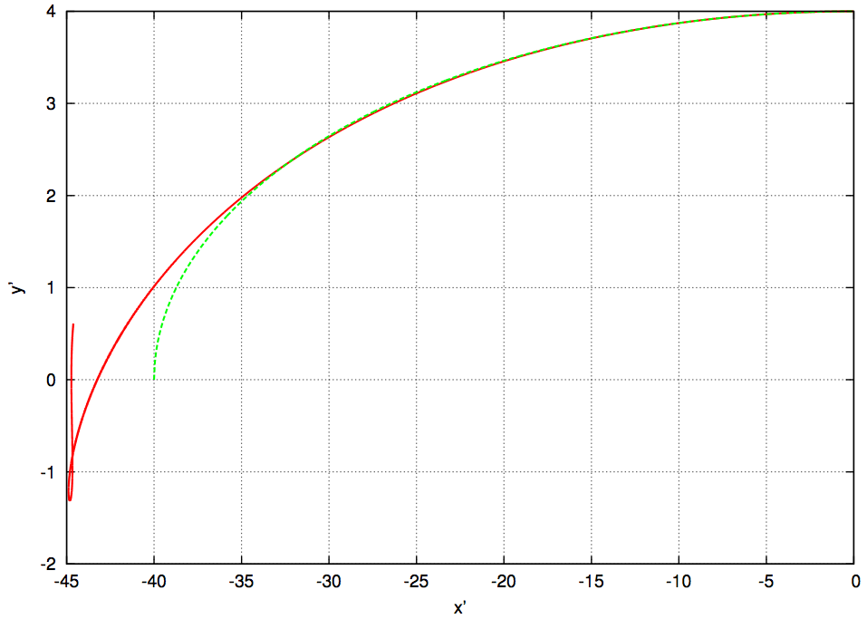
Figure 1: Electron trajectory for $\gamma_{p}=10$ and for the initial conditions $x^{\prime}(0)=0$, $y^{\prime}(0)=4$, $\dot{x}^{\prime}(0)=p_{x0}^{\prime}$, $\dot{y}^{\prime}(0)=0$ [where $p_{x0}^{\prime}$ is chosen as the solution of Eq. (10)]. The numerical solution of Eqs. (1) and (2) is in solid red line, while the elliptical trajectory is in dashed green line.

It is easily seen that the real trajectory does not follow an ellipse. We checked that errors due to finite time step and numerical truncation were negligible; varying the time step or the level of truncation has no effect on the result. The trajectory is also found not to be sensitive to initial conditions, for the time scale of interest. Moreover, we performed a cross-verification of both the analytical and numerical calculations. The Taylor expansion is valid only for $\tau\ll 1$, and the time required for the electron to reach the back of the bubble is, in orders of magnitude, $\tau\sim\gamma_{p}r_{b}/|p_{x0}|^{\prime}\sim r_{b}^{1/3}$. Therefore we need $r_{b}^{1/3}\ll 1$ for the expansion to be valid on the length scale of interest (the bubble extension). On Fig. 2 is represented both the analytical Taylor expansion [given by Eqs. (4), (5) and (8)] and the numerically integrated trajectory [solution of Eqs. (1) and (2)], up to $\tau=0.5$, for $r_{b}=0.01$ and $\gamma_{p}=10$. The choice $r_{b}=0.01$ is only used here to perform a verification between analytical and numerical calculations (but this case does not have any physical relevance since the bubble model makes sense only for $a_{0}>2$, i.e. for $r_{b}>2\sqrt{2}$).

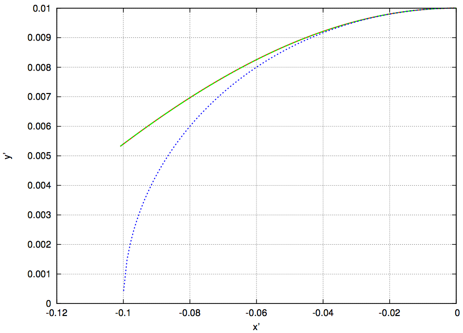
Figure 2: Electron trajectory for $\gamma_{p}=10$ and for the initial conditions $x^{\prime}(0)=0$, $y^{\prime}(0)=0.01$, $\dot{x}^{\prime}(0)=p_{x0}^{\prime}$, $\dot{y}^{\prime}(0)=0$ [where $p_{x0}^{\prime}$ is chosen as the solution of Eq. (10)]. The numerical solution of Eqs. (1) and (2) is in solid red line, while the Taylor expansion of the solution, given by Eqs. (4), (5) and (8), is in dashed green line (superposed to the red line). The elliptical trajectory is in dotted blue line. Trajectories are plotted up to $\tau=0.5$.

Both trajectories are very close to each other, confirming both the analytical and numerical calculations.

We conclude that the real trajectory is not elliptical, whatever the initial conditions. We will see in the Discussion section why incorrectly considering the trajectory as elliptical leads to erroneous conclusions.

II On the error of KNPS

Thomas argues that in the work of KNPS, the approximations made in Eqs. (4) to (7) of Ref. Kostyukov et al. (2009) are too restrictive and fail to correctly predict the self-injection threshold. This can be easily understood by regarding at Eq. (6) of Ref. Kostyukov et al. (2009): $X$ necessarily decreases, even when $P_{x}\rightarrow\infty$ (in the notation of Ref. Kostyukov et al. (2009), $X=\xi/r_{b}=(x-v_{p}t)/r_{b}$, $P_{x}=p_{x}/r_{b}^{2}$). Such equations can not describe the injection, since when the electron is injected, $X$ is increasing. Nevertheless, Eqs. (4) to (7) of Ref. Kostyukov et al. (2009) are only used to obtain the numerical coefficient $P_{x}\simeq 1.1$ at the moment where $p_{y}=0$ for the first time, and to insert it into Eq. (3). The KNPS threshold is based on the conservation of the hamiltonian $\mathcal{H}$ between the initial time and the critical time where $p_{y}=0$ for the first time, and no approximation is needed in this approach. From that, Eq. (3) of Ref. Kostyukov et al. (2009) is established. Moreover, a simple analysis in orders of magnitude of the equations of motion Eqs. (1) and (2) of Ref. Kostyukov et al. (2009) shows that $p_{x}\propto r_{b}^{2}$. Inserting this behavior in Eq. (3) of Ref. Kostyukov et al. (2009) demonstrates the self-injection threshold of Eq. (9) in Ref. Kostyukov et al. (2009), but without the numerical coefficient. The numerical coefficient can then be evaluated by drastically simplifying the equations of motion, as done by KNPS. In reality, the coefficient could have a very weak dependance on the parameters $r_{b}$ and $\gamma_{p}$, since the real equations depend on them.

Therefore, the arguments of Thomas concerning the error of KNPS do not hold, and the semi-analytical derivation of KNPS is correct.

III Numerical threshold

In order to verify the mathematical validity of the self-injection thresholds proposed either by Thomas or KNPS, we have integrated the equations of motion and scanned all the parameter space $(r_{b},\gamma_{p})$, with the same initial conditions as Thomas or KNPS, i.e. $x^{\prime}(0)=0$, $y^{\prime}(0)=r_{b}$, $\dot{x}^{\prime}(0)=-\gamma_{p}v_{p}$, $\dot{y}^{\prime}(0)=0$ (electron at rest in the laboratory frame). The electron is considered to be injected if $r^{2}=x^{\prime}{{}^{2}}/\gamma_{p}^{2}+y^{\prime}{{}^{2}}\leqslant r_{b}^{2}$ at all time steps. Note that if the electron escapes the bubble before $y=0$, it will never come back inside, so that imposing the condition $r\leqslant r_{b}$ only when $y\leqslant 0$ gives the same result. The numerical result is presented on Fig. 3 and is in agreement with the work of KNPS. In the frame of the model considered by KNPS and Thomas (with initial conditions corresponding to an electron at rest in the laboratory frame), the threshold is written $r_{b}>1.30\gamma_{p}$.

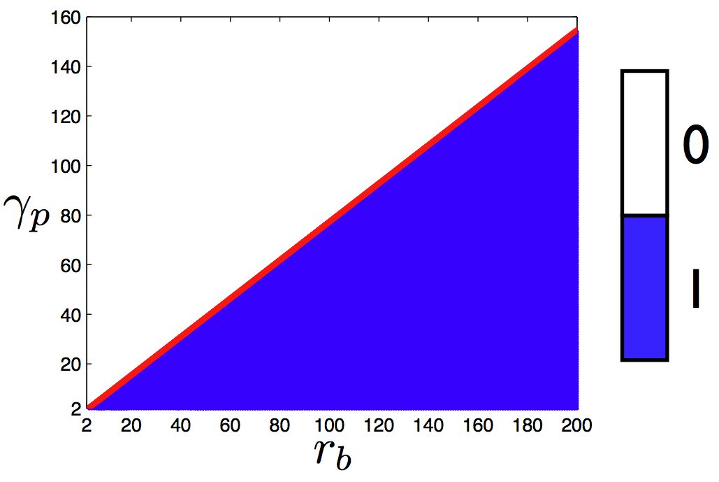
Figure 3: For each value of $r_{b}$ and $\gamma_{p}$, a value of 1 is displayed if the electron is injected and 0 otherwise. The initial conditions are $x^{\prime}(0)=0$, $y^{\prime}(0)=r_{b}$, $\dot{x}^{\prime}(0)=-\gamma_{p}v_{p}$, $\dot{y}^{\prime}(0)=0$ (electron at rest in the laboratory frame), and a trajectory is considered injected if $r\leqslant r_{b}$ at all time steps. The frontier between injected and non-injected trajectories follows a line of equation $\gamma_{p}=0.77\;r_{b}$ (plotted in red line), whose numerical coefficient is very close to the value obtained by KNPS Kostyukov et al. (2009).

IV Discussion

In this comment, we have analyzed the mathematical validity of the results proposed either by Thomas and KNPS, considering a particular model where the bubble is considered perfectly spherical and described by prescribed electromagnetic fields. However, it is clear that such a simple model can potentially fail to correctly describe the physical mechanisms present in the blow-out regime of laser-plasma interaction. In the work of KNPS Kostyukov et al. (2009), only one PIC simulation has been performed, while several simulations with very different parameters should be performed to confirm the linear self-injection threshold. In addition, we highlight that, while Thomas considers the parameter $\gamma_{p}$ as a direct function of the electron plasma density $\gamma_{p}\propto n_{e}^{-1/2}$, it should be instead considered as the bubble back gamma factor which can be much lower due to the time evolution of bubble. Indeed, Kostyukov and co-workers included the rate of bubble expansion in the bubble back gamma factor Kostyukov et al. (2010) and found similar results that those of Kalmykov et al. Kalmykov et al. (2009), which have explicitly studied electron injection inside a time-dependent bubble. This bubble back gamma factor has to be properly taken into account if we want to verify the linear self-injection threshold of KNPS by PIC simulations.

We have seen that, contrary to the Thomas’ affirmation, there is no elliptical solution for Eqs. (1) and (2). The difference between the result of Thomas and the linear self-injection threshold of KNPS can be understood as follows. In the bubble frame, the hamiltonian is written $\mathcal{H}^{\prime}=\gamma^{\prime}-\phi^{\prime}$, where $\phi^{\prime}\simeq 2\gamma_{p}\phi=-\gamma_{p}r^{2}/4$, $\phi^{\prime}$ and $\phi$ being the scalar potential respectively in the bubble and laboratory frame. The model is time-independant in the bubble frame, therefore $\mathcal{H}^{\prime}$ is conserved and $\gamma^{\prime}+\gamma_{p}r^{2}/4=\gamma_{0}^{\prime}+\gamma_{p}r_{b}^{2}/4$ [this is Eq. (9) of Ref. Thomas (2010)]. Because $\gamma^{\prime}\geqslant 1$, there is a maximal value for $r$, which is given by $r_{\textrm{max}}\simeq r_{b}(1+4/r_{b}^{2})^{1/2}$ for $\gamma_{p}\gg 1$ and $\gamma_{0}^{\prime}\simeq\gamma_{p}$. For large values of $r_{b}$, $r_{\textrm{max}}$ becomes very close to $r_{b}$, and if a small error is committed, an electron can be seen injected while it is not in the frame of the considered model. Thomas used Eq. (7), considering $\gamma^{\prime}$ as a constant (which is equivalent as saying that the trajectory is elliptical, according to the conservation of $\mathcal{H}^{\prime}$), and studied the motion in terms of the $x^{\prime}$ and $p_{x}^{\prime}$ variables. In reality, $\gamma^{\prime}$ is not constant along the trajectory, which induces some degree of error in the calculation of the relation between $x^{\prime}$ and $p_{x}^{\prime}$, given by Eq. (20) of Ref. Thomas (2010). In fact, the difference in the result of Thomas arises when he considered an electron to be injected if $x^{\prime}\geqslant-\gamma_{p}r_{b}$ when $p_{x}^{\prime}=0$, implicitly assuming an elliptical trajectory, for which $y^{\prime}=0$ and $|x^{\prime}|/\gamma_{p}=r$ when $p_{x}^{\prime}=0$, such that the condition $|x^{\prime}|/\gamma_{p}\leqslant r_{b}$ is equivalent to $r\leqslant r_{b}$. But because the trajectory is not elliptical, when $p_{x}^{\prime}=0$, $y^{\prime}\neq 0$ and $|x^{\prime}|/\gamma_{p}\neq r$ such that even if $r_{b}<r\leqslant r_{\textrm{max}}$ (the electron is not injected), we can have $|x^{\prime}|/\gamma_{p}\leqslant r_{b}$. For large $r_{b}$, even if $r=r_{\textrm{max}}$ when $p_{x}^{\prime}=0$, because $r_{\textrm{max}}$ is very close to $r_{b}$, $|x^{\prime}|/\gamma_{p}$ will be smaller than $r_{b}$ due to the non-zero value of $y^{\prime}$. For example, for $r_{b}=12$ and $\gamma_{p}=200$, according to Thomas the electron is injected, while it is not according to KNPS. Figure 4 displays the corresponding trajectory (with initial conditions for an electron at rest in the laboratory frame) and the ellipses of equation $r=r_{b}$ and $r=r_{\textrm{max}}$.

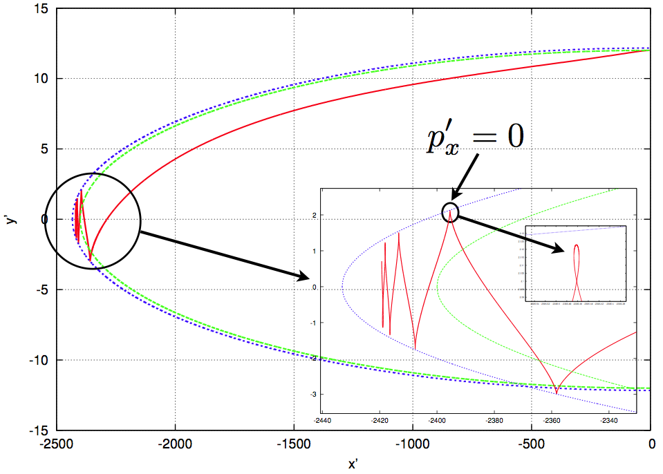
Figure 4: Numerically integrated electron trajectory for $\gamma_{p}=200$ and for the initial conditions $x^{\prime}(0)=0$, $y^{\prime}(0)=12$, $\dot{x}^{\prime}(0)=-\gamma_{p}v_{p}$, $\dot{y}^{\prime}(0)=0$ (electron at rest in the laboratory frame), in solid red line. The ellipse of equation $r=r_{b}$ is in dashed green line, and the ellipse of equation $r=r_{\textrm{max}}$ is in dotted blue line. The inset displays a zoom of the back of the bubble and shows the point where $p_{x}^{\prime}=0$ for the first time. At that point, $r\simeq r_{\textrm{max}}\geqslant r_{b}$ and $|x^{\prime}|/\gamma_{p}\leqslant r_{b}$.

At the moment where $p_{x}^{\prime}=0$ for the first time, $r\simeq r_{\textrm{max}}>r_{b}$ (it is considered as non-injected by KNPS), whereas $|x^{\prime}|/\gamma_{p}\leqslant r_{b}$ (it is injected according to the Thomas’ criterion). This example highlights that because $r_{b}$ and $r_{\textrm{max}}$ are very close to each other, a small error in the derivation or in the criterion can considerably change the conclusion (injected or non-injected). In addition, in that case, it is clear that $\gamma^{\prime}$ is not constant at all, since it almost attains $\gamma^{\prime}=1$ (when $r\simeq r_{\textrm{max}}$) and it attains very large values $\gamma^{\prime}\gg\gamma_{0}^{\prime}$ during the period where the electron is inside the bubble.

We have performed a complete scan of the parameter space $(r_{b},\gamma_{p})$, as for Fig. 3, but applying either the condition $r\leqslant r_{b}$ or $|x^{\prime}|/\gamma_{p}\leqslant r_{b}$ at the moment where $p_{x}^{\prime}=0$ for the first time. For the condition $r\leqslant r_{b}$, the result is similar to Fig. 3 but with a slightly different numerical coefficient, the threshold being $r_{b}>0.95\gamma_{p}$. For the Thomas’ condition, $|x^{\prime}|/\gamma_{p}\leqslant r_{b}$, the result is non-trivial and is displayed on Fig. 5.

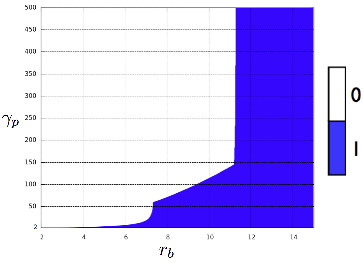
Figure 5: For each value of $r_{b}$ and $\gamma_{p}$, a value of 1 is displayed if $|x^{\prime}|/\gamma_{p}\leqslant r_{b}$ at the moment where $p_{x}^{\prime}=0$ for the first time, and 0 otherwise. The initial conditions are $x^{\prime}(0)=0$, $y^{\prime}(0)=r_{b}$, $\dot{x}^{\prime}(0)=-\gamma_{p}v_{p}$, $\dot{y}^{\prime}(0)=0$ (electron at rest in the laboratory frame).

According to this criterion, self-injection occurs for much larger values of $\gamma_{p}$ than for the KNPS threshold. But there is no physical meaning for applying $|x^{\prime}|/\gamma_{p}\leqslant r_{b}$ as a criterion for self-injection. As we can see on Fig. 4, the electron streams backwards after the point where $p_{x}^{\prime}=0$ and $|x^{\prime}|/\gamma_{p}\leqslant r_{b}$. It should not be considered as injected in the frame of the considered model. Therefore, the threshold for self-injection indicated in Eq. (22) of Ref. Thomas (2010) is incorrect, because it relies on the elliptical trajectory which is in contradiction with the equations used to derive the threshold.

Nevertheless, the present discussion emphasizes that, because when $r_{b}$ increases $r_{\textrm{max}}$ becomes very close to $r_{b}$, a small deformation of the bubble structure, or the consideration of the field enhancement at the back of the bubble due to electron crossing, or the consideration of self-consistent screened fields, could considerably change the conclusion about injection or non-injection in the bubble. Considering these effects in the model and confirming or invalidating the KNPS result are areas for future works.

References

- Thomas (2010) A. G. R. Thomas, Phys. Plasmas, 17, 056708 (2010).
- Kostyukov et al. (2009) I. Kostyukov, E. Nerush, A. Pukhov, and V. Seredov, Phys. Rev. Lett., 103, 175003 (2009).
- Kostyukov et al. (2010) I. Kostyukov, E. Nerush, A. Pukhov, and V. Seredov, New J. Phys., 12, 045009 (2010).
- Kalmykov et al. (2009) S. Kalmykov, S. A. Yi, V. Khudik, and G. Shvets, Phys. Rev. Lett., 103, 135004 (2009).