Effects of noise on models of spiny dendrites

Abstract

We study the effects of noise in two models of spiny dendrites. Through the introduction of different types of noise to both the Spike-diffuse-spike (SDS) and Baer-Rinzel (BR) models we investigate the change in behaviour of the travelling wave solutions present in the deterministic systems, as noise intensity increases. We show that the speed of wave propagation in the SDS and BR models respectively decreases and increases as the noise intensity in the spine heads increases. Interestingly the discrepancy between the models does not seem to arise from the type of active spine head dynamics employed by the model but rather by the form of the spine density used. In contrast the cable is very robust to noise and as such the speed shows very little variation from the deterministic system.

We look at the effect of the noise interpretation used to evaluate the stochastic integral; Itô or Stratonovich and discuss which may be appropriate. We also show that the correlation time and length scales of the noise can enhance propagation of travelling wave solutions where the white noise dominates the signal and produces noise induced phenomena.

1 Introduction

The neuron, or nerve cell, is the building block of the mammalian nervous system; it sends, receives and processes information that ultimately controls functions as fundamental as our breathing and as complex as memory. The neuron comes in many forms depending on which area of the brain it occupies and its function but all neurons share the same basic structure. We are interested in models of spiny dendritic tissue and the effects of noise on these signal processing capabilities. The dendritic tree allows a greater surface area for synaptic connections and around $90\%$ of excitatory synapses in the brain are made onto dendritic spines. Dendrites are typically 1-2 mm long and the dendritic spines are small bulbous protrusions of 1-2 $\mu$m long. Spiny dendrites occur in many regions of the brain e.g. CA1 and CA3 pyramidal neurons in the hippocampus (important in long term memory), basal ganglia (used in motor control and learning) and spiny stellate neurons in the cerebral cortex (also important in memory) [29], [31], [1]. The spines are thought to be an important component in signal propagation and computations along the dendrite and spine motility and morphology, called spine plasticity, is thought to be an important process in learning and memory, [33], [7], [3] and [15]. In the models investigated here the plasticity can be related to physical properties of the dendritic tissue such as the spine stem resistance and spine density. The advent of the confocal and two-photon microscopy used to image the membrane in dendrites allowed the measurement of action potentials (APs) in dendrites and proved that action potentials can be generated in the dendrites themselves. These techniques made it possible to compare experimental, [14], [33], and theoretical results, [24], [25], that predict how voltage will spread throughout a length of dendrite, or a branched dendritic structure, also see for a review [27].

We consider voltage spread throughout a length of spiny dendrite as a wave propagating from the spines at the distal end, through the main body of the dendrite to the soma without including the effect of the soma. This is an interesting problem as much information processing may occur prior to the action of the soma, see review [20]. We use two dendritic models that describe voltage evolution in a length of spiny dendrite: the Baer-Rinzel (BR) model, [2], and the Spike-Diffuse-Spike (SDS) model, [4], [5]. Both these models couple active spines to a passive cable through a spine density which is a constant, continuum value in the original BR model and equally distributed point attachments in the SDS model. We extend the BR model to include a spatially dependent spine density which can be controlled through one parameter; the density is equivalent to a continuum in one limit and to the point attachment in the other. In this way we investigate the importance of the spine stem area on the propagation of waves in the dendrite models. We consider the effect of random fluctuations, or noise, in the BR and SDS models. There are two types of noise in a neural system, intrinsic and extrinsic noise, [13], [19], (see [10] for overview of noise in all levels of the central nervous system). Intrinsic noise is a source of noise which is always present in the system and thermal noise is one example. Another source of intrinsic noise, which may be considered particularly relevant in spiny dendrites, is the process of synaptic gating since the release of the neurotransmitter is a stochastic process. The second type of noise, extrinsic, emanates from out with the cell itself and one source is other, nearby neurons. One interpretatoin of the correlation length associated with our spatially correlated noise is the length scale over which signals as inputs are transmitted. We see that there are length scales that promote propagation.

2 The models for spiny dendrites

2.1 Spike Diffuse Spike model

The SDS model [4], [5] and [30] describes a length of spiny dendritic by coupling a passive dendrite to active spines. The cable is modelled by the passive cable equation, and the spine head dynamics by the leaky integrate and fire model with an imposed refractory time $\tau$. The spines are attached at discrete points along the cable by a spine stem with resistance, $r$. The points at which the spines are attached can be spaced with any spatial distribution but here we have chosen equally spaced points.

The membrane potential in the cable, V(x, t), is given by:

$$\frac{\partial V}{\partial t}=D\frac{\partial^{2}V}{\partial x^{2}}-\frac{V}{\tau}+{Dr_{a}\rho(x)\frac{\hat{V}-V}{r}}+(\mu+\nu g(V))\ast\frac{\partial Z(t)}{\partial t}$$ (1)

with sealed end boundary conditions, $D=\frac{\lambda^{2}}{\tau}$ is the diffusion coefficient, $\tau=r_{m}c_{m}$ is the membrane time constant, $\lambda=\sqrt{\frac{dr_{m}}{4r_{a}}}$ is the electronic space constant, $r_{a}$ is the intracellular resistance per unit length, $x\in[0,L]$ and $t\in[0,T]$, $L$ is the length of the cable and $T$ is the final time. We take $Z$ to either be a space-time Wiener process $Z=W(x,t)$ chosen to satisfy the form of spatially correlated noise we require or we take $Z(t)=K(t)$ a white noise or temporally correlated noise path that is constant in space. We use $\ast$ to denote that the stochastic integral can be interpreted in either an Itô or Stratonovich sense and it will be expressed by the usual convention: $\int g(V)dW$ or $\int g(V)\circ dW$ respectively where appropriate. $\rho(x)=\sum_{n\in\Gamma}\delta(x-x_{n})$ is the density of spines, attached at discrete points $x_{n}$, $\hat{V}(x_{n},t)$ is the action potential produced by the spine at the point $x_{n}$, the form of the action potential is free to be chosen, and $r$ is the spine stem resistance.

The spine head dynamics are modelled by the stochastic leaky integrate and fire (IF) model, upto firing threshold:

$$\frac{dU_{n}(t)}{dt} = \frac{V_{n}(t)}{\hat{C}r}-\epsilon U_{n}(t)-\underbrace{\hat{C}h\sum_{m}\delta(t-T_{n}^{m})}_{\textrm{Reset}}+(\mu+\nu g(U_{n}(t)))\ast\frac{dZ_{n}(t)}{dt}.$$ (2)

We take $Z$ to either be constant in space $Z_{n}(t)=K_{n}(t)$, where $K_{n}$ is either a white noise or temporally correlated path or $Z_{n}=W_{n}$ a spatially correlated Wiener process evaluated at each spine at $x_{n}$. We choose the form of the multiplicative noise term to preserve the range of voltage $[0,1]$: $g(U)=U(1-U)$ while $U\in[0,1]$ and zero otherwise, [9]. $\hat{C}$ is the capacitance, $r$ the spine stem resistance and $\epsilon=\frac{1}{\hat{C}}\left(\frac{1}{r}+\frac{1}{\hat{r}}\right)$, with $\hat{r}$ as the membrane resistance of the spine head. The m-th firing time of the nth spine, $T_{n}^{m}$, is governed by the integrate and fire process:

$$T_{n}^{m}=\inf\{t|U_{n}(t)\geq h,t>T_{n}^{m-1}+\tau_{R}\}\textrm{ ,}$$ (3)

where $\tau_{R}$ is the refractory time period, during which the spine is unable to fire. This refractory time is introduced to mimic the dynamics of the Hodgkin-Huxley (HH) model, which has a natural refractory time. At $U_{n}=h$ an action potential is injected into the cable; the form of this injected potential can be chosen to be a suitable function, in the SDS model described here, the function was chosen to be a rectangular pulse, given by:

$$\eta(t)=\eta_{0}\Theta(t)\Theta(\tau_{s}-t)\textrm{ ,}$$ (4)

where $\Theta(t)$ is the Heaviside function, $\tau_{s}$ is the length of time the pulse lasts for and $\eta_{0}$ is the strength (magnitude) of the pulse.

These equations describing the dynamics of spiny dendritic tissue can be solved using a combination of analytical and numerical techniques, see [30] for a full description of the methodology.

The solution of this problem shows that the deterministic SDS model supports the propagation of saltatory travelling waves along the length of the cable [5] and [30] provides a preliminary investigation to these solutions with some noise in the system but does not compare the speed of propagation or the effect of spatial correlations.

2.2 Baer-Rinzel model

The Baer-Rinzel (BR) model, [2], describes the voltage evolution of a spiny dendrite using the Hodgkin Huxley (HH) equations to describe the active properties of the spine heads: the voltage $U$ in the spine heads and the gating variables $m,n,h$. They are coupled, with a certain density $\rho(x)$, to a uniform passive cable, whose voltage, $V$, is modelled by the passive cable equation.

We choose to include noise only to the m-dynamics since the other gating variables are very sensitive to the noise and the m-gate is the dominant variable as seen in reductions of the Hodgkin Huxley dynamics to a two variable system, e.g. Fitzhugh Nagumo model, [26] and [13]. The equations for the stochastic BR model we consider are given by three deterministic equations:

$$\hat{C}\frac{\partial U}{\partial t} = g_{K}n^{4}(V_{K}-U)+g_{Na}hm^{3}(V_{Na}-U)+g_{L}(v_{L}-U)-\frac{U-V}{r}$$ (5)

$$\frac{dX}{dt} = \alpha_{X}(1-X)-\beta_{X}X\textrm{ ,}$$ (6)

where $X\in[n,h]$. Along with

$$C\frac{\partial V}{\partial t} = -g_{L}(V-V_{L})+\frac{1}{r_{a}\pi d}\frac{\partial^{2}V}{\partial x^{2}}+\rho(x)\frac{U-V}{r}+(\mu_{c}+\nu_{c}g_{c}(V))\ast\frac{\partial Z(x,t)}{\partial t}$$ (7)

$$\frac{dm}{dt} = \alpha_{m}(1-m)-\beta_{m}m+(\mu_{m}+\nu_{m}g_{m}(m))\ast\frac{dZ_{m}}{dt}\textrm{ ,}$$ (8)

the $\mu$’s give the strength of additive noise and the $\nu$’s the strength of the multiplicative noise. We take either $Z(t)$=$K(t)$ is a constant in space and either white or correlated in time or $Z(x,t)=W(x,t)$ for a spatially correlated Wiener processes. Note that the equations for $X\in[m,n,h]$ and $U$ are coupled together, at each point in space, by the cable or by the noise if it is spatially correlated in the m-dynamics.

When the noise is multiplicative (extrinsic), the stochastic integral can be interpreted in either an Itô or Stratonovich sense and we use the standard notation conventions: $\int g(V)dW$ for Itô and $\int g(V)\circ dW$ for Stratonovich. The Stratonovich interpretation is often used in cases where the noise is fluctuating on a much faster scale than the system dynamics. The integrand $g(V)$ is evaluated at the mid-point of the interval i.e. $\frac{g(V(t))+g(V(t+\Delta t))}{2}$, where $\Delta t$ is the time step and so the Stratonovich interpretation can be thought of as averaging this fast behaviour in some way over the time interval. However if the time-scales are much closer and the system responds to the noise on a similar time-scale then the Itô interpretation is more appropriate since it is non-anticipating, evaluating at the left hand end point of the time interval, [23], [16]. Itô calculus is favoured in biological and financial applications due to this non-anticipating property i.e. only historical information is usually available. Despite this general assumptions each case should be considered individually, e.g. the results presented in [17] show that simulations using a Stratonovich interpretation are in closer agreement with the analytically predicted firing rates of a simple model of a type I neuron. Here we present results, [6], which differ depending on the noise interpretation used. It could be possible to use this discrepancy to determine the appropriate stochastic calculus for wave propagation in spiny dendrites. We choose the multiplicative noise functions $g$, in each of the equation to ensure the fluctuations are added correctly to the resting state of $V$ and $m$. With this in mind we choose the functions of the multiplicative noise to be: $g_{c}(V)=-(65+V)$ and $g_{m}(m)=m(1-m)$ when $m\in[0,1]$ and zero otherwise.

The spine density, $\rho(x)$ can be a constant as in the original BR model [2] which has been shown to support travelling waves, solitary, multi-bump and periodic waves, [18].

We extend the model here and consider here spatially dependent density, which has a parameter, $\kappa$, to control the area of the spine stem attached to the cable. For spines centered at spatial points $x_{n}$:

$$\rho(x)=\sum_{n}\rho_{max}\xi_{n}\exp(-\kappa(x-x_{n})^{2})\textrm{ .}$$ (9)

Here we have $\rho_{max}$ is the maximum value of the density, taken to be the value used for the original BR model, and

$$\xi_{n}=\left\{\begin{array}[]{ll}1&\textrm{ if $x_{n}-\frac{d}{2}<x\leq x_{n}+\frac{d}{2}$}\\ 0&\textrm{ otherwise,}\end{array}\right.$$

where $d$ is the spine spacing and $\kappa\in\mathbb{R}^{+}$ controls the width of the spine stem. As $\kappa\to 0$, $\rho(x)\to\rho_{max}$ and as $\kappa\to\infty$, $\rho(x)\to\sum_{n}\rho_{max}\delta(x-x_{n})$. Therefore at the $\kappa\to 0$ limit the model is the BR model and at $\kappa\to\infty$ limit the model resembles the SDS model with HH dynamics (instead of IF) in the spine heads.

2.3 Noise generation

We use space/time white noise, temporally correlated and spatially correlated noise throughout the simulations to investigate the effects of noise on signal propagation in the previously described dendrite models. We consider a temporally correlated noise generated by the Ornstein-Uhlenbeck process, given as:

$$dK(t)=\beta(\theta-K(t))dt+\sigma db(t)\textrm{,}$$ (10)

where $K(t)$ is a stochastic process called the Ornstein-Uhlenbeck process, $\beta$ is a parameter which can adjust the time scale of the correlation, called the mean reversion rate, $\theta$ is the mean to which the process will revert to if given enough time, $\sigma$ is another parameter which is called the volatility and $b$ is a Brownian motion. To get a white noise path we simply set $\beta=1$ and $\sigma=1$.

The generation of a spatial correlated noise is introduced by a process described in e.g. [28] and [11]. This form of the spatially correlated noise is chosen to satisfy chosen properties of the correlation length; we require that the correlation is over a short range since we would not expect interference between distant spines but would expect neighbouring spines to affect each other. We define a Q-Wiener process by the sum:

$$W(x,t)=\sum_{j\geq 0}\lambda_{j}^{\frac{1}{2}}(x)\mathbf{e_{j}}(x)b_{j}(t)\textrm{ .}$$ (11)

Assuming that $Q$ has the same eigenfunctions as the Laplacian (and assuming Neumann boundary conditions on $[0,L]$), $\Delta$, $\mathbf{e_{j}}(x)=\sqrt{\frac{2}{L}}\cos(\frac{\pi jx}{L})$ where $j=1,2,3,\dots$ and $\mathbf{e_{0}}(x)=\sqrt{\frac{1}{L}}$, $b_{j}(t)$ are standard Brownian motions and $\lambda_{j}$ are eigenvalues of $Q$ which we choose here to satisfy a form of spatial correlation. We choose a correlation such that the noise is white in time and has an exponential correlation in space of length is $\zeta$ (to satisfy the assertion that nearby spines have more influence than distant). The covariance and correlation function are given by and

$$\mathbb{E}(W(x,t)W(x^{\prime},t^{\prime})) = F_{c}(x-x^{\prime})\min\{t,t^{\prime}\}$$ (12)

$$F_{c}(x) = \frac{1}{2\zeta}\exp(-\frac{\pi x^{2}}{4\zeta^{2}})\textrm{ .}$$ (13)

Using this form of the correlation function we obtain [6] the following form for the eigenvalues of $Q$: $\lambda_{j}=\exp(-\frac{\pi j^{2}\zeta^{2}}{2L^{2}})$. If we require a noise which is white in space and time we can use $Q=I$, this is non-trace class but has the eigenvalues $\lambda_{j}=1$, $\forall j$ and as such the sum reduces to: $W(x,t)=\sum_{j=1}^{\infty}e_{j}(x)b_{j}(t)$. The correlation length $\zeta$ can be chosen such that the strongest effect of the correlation is felt over neighbouring spines and not, for example, the entire length of the cable. Since we have chosen the form of the correlation to ensure nearby spines have more influence on neighbours than distant spines it would be counterproductive to use a long correlation scale. We investigate by the correlation length the effect of correlated signals into the dendrite as indicated in the introduction.

In order to simulate the different interpretations of the noise we require different numerical schemes. In the case of an Itô interpretation we use the Euler-Maruyama method and for the Stratonovich interpretation we use the stochastic Heun method, for details on the implementation of these methods see [6].

2.4 Speed of propagation of stochastic wave

We rescale computed speeds by the deterministic speed, $c_{det}=\frac{d}{t}$, where $d$ is the distance travelled along the cable and $t$ is the time the wave takes to travel this distance; thus the plotted speeds are given by $c=\frac{c_{noisy}}{c_{det}}$. This rescaling allows comparison of the different models which have different absolute values for the speed; it also makes it easy to see in the graphs if the wave is speeding up ($c>1$) or slowing down ($c<1$), with respect to the deterministic wave speed, [6]. In order to find the speed of any stochastic travelling wave propagating on the cable we find the times, $t_{1}$ and $t_{2}$, at which the wave crosses two points, $x_{1}$ and $x_{2}$, along the cable and use:

$$c_{noisy}=\frac{x_{2}-x_{1}}{t_{2}-t_{1}}\textrm{.}$$ (14)

If the wave fails to reach $x_{2}$ then we say that the wave has failed to propagate, [6]. Failure is determined by the size of the voltage in the cable at point $x_{2}$; if $V(x_{2},t)\geq\theta$, $\theta$ is a threshold value chosen from the voltage values in the deterministic case, then it is still propagating. The threshold value must be large enough that the voltage will only reach this level if the voltage is close to that of the deterministic system and so we avoid the case where the propagation is purely noise induced, i.e. we are not measuring small fluctuations induced by noise only but we do see the underlying signal too. We also impose the condition that the wave must travel sequentially, i.e. each spine must fire in spatial order from distal to proximal end of the dendrite.

3 Effects of the noise on speed of propagation

Here we look at the results of the measuring the average speed of the waves in the noisy BR and SDS models, over 100 realisations and for the parameter values in Figure 5. We consider white noise, temporally correlated noise and spatially correlated noise in both the spine heads and the cable of each model (the noise is in the m-dynamics for the BR model). We show error bars that represent the standard deviation around the mean value of speed for each value of noise intensity ($\pm\textrm{S.D.(c)}=\sqrt{\mathbb{E}(c^{2})-\left(\mathbb{E}(c)\right)^{2}}$). Table 5 contains the parameter values taken and their units.

3.1 Effect of multiplicative noise in the BR and SDS models

The following results show the effect of multiplicative noise in both models interpreted in the Itô sense.

(a)	(b)
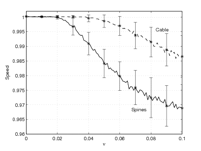
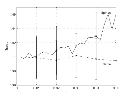
(c)	(d)

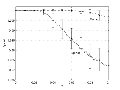
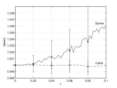
Figure 1: This figure shows how the speed of propagation changes as the noise intensity increases for both the SDS and BR models. Each plot shows the effect of noise in both the spines (solid lines) and the cable (dotted lines); the error bars are $\pm$ the standard deviation and get larger as the noise intensity increases. Plot (a) shows that space-time white noise in the spine and cable dynamics of the SDS model reduces the speed of propagation, much more so when the noise is in the spine heads. Plot (b) shows that white noise in the BR model increases the speed of propagation when the noise is driving the m-dynamics and that the cable is robust to this noise as the speed changes little with noise intensity. Plot (c) shows the SDS model driven by temporally correlated noise in the spine and cable dynamics and again the cable is more robust than the spines to the noise. As the noise intensity increases the speed of propagation decreases. Plot (d) shows the speed of propagation in the BR model increasing with temporally correlated noise intensity when the noise is in the m-dynamics, again the cable seems robust to the effects of noise.

Figure 1 shows that there is a difference in the behaviour of the two models under the influence of synaptic noise (i.e. multiplicative noise driving the spine dynamics); the speed of propagation in the SDS model decreases as noise intensity increases and the speed increases in the BR model with an increase in noise intensity. In both cases the cable is more robust to the noise and there is little or no variation in the speed as the noise intensity in the cable increases. We can interpret this to mean that the synaptic noise/noise in the input signal to be more important than background noise in the propagation of signals in spiny dendrites. Since the effect in the cable is negligible compared to the effect in the spines we consider only the spines from now on.

We look at the effect of spatially correlated noise in the models, again we look at the noise added to the m-dynamics for the BR model and spine dynamics for the SDS model. Figure 2 shows the effect of spatially correlated multiplicative noise on the speed of propagation in the models as the noise intensity increases. We have used both an Itô and Stratonovich interpretation to compare the different noise models. The type of noise integral used in the evaluation of the stochastic models has no qualitative effect on the behaviour of the stochastic waves when the noise is white or OU but when the noise is spatially correlated we observe a difference in the behaviour for both models when the noise interpretation changes. Figure 2, plot (a) shows, for Itô interpretation, that the speed of a stochastic wave does not change, but for the SDS model the speed decreases (as for white and OU noise). Plot (b) shows an increase in speed for both the BR and SDS model, therefore the choice of calculus when the noise is spatially correlated is important, although it does not explain the difference in behaviour for white or OU noise.

(a)	(b)

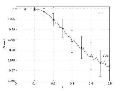
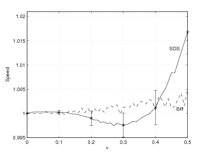
Figure 2: This figure shows the effect of spatially correlated noise in the spine dynamics of both models. Plot (a) shows effect of the Itô interpretation of the noise in the SDS model (solid line) and the BR model (dashed line). We observe a reduction in the speed as the noise intensity increases for the SDS model but no change for the BR model. Plot (b) shows the effect of the Stratonovich interpretation of the noise in the SDS model (solid line) and BR model (dashed line). Both models show an increase in speed as the noise intensity increases, although the SDS model shows a larger increase.

3.2 Small spatially correlated noise analysis of the BR model

When we consider the noise to be interpreted by the Stratonovich calculus we can implement a small noise expansion that exploits the non-zero mean of the noise term. This expansion of the stochastic BR model, equations (5-7), to approximate the behaviour of the system without having to simulate or solve any Stratonovich stochastic integrals. We use this approach for the original BR model since the constant density makes the model amenable to analysis with the continuation package AUTO-07P, [8]. This approach follows the working of [11] and [12] and the expansion is a standard perturbation approach. Applying this method to the stochastic BR model, Equation (7) and converting to the travelling wave frame, using the standard anzatz $\xi=ct-x$, where $c$ is the wave speed, we obtain:

$$V_{\xi} = \hat{W}$$ (15)

$$CcV_{\xi} = -g_{L}(V-V_{L})+\frac{1}{r_{a}\pi d}V_{\xi}+\rho\frac{U-V}{r}-\nu_{c}^{2}F_{c}(0)(65+V)$$ (16)

$$c\hat{C}U_{\xi} = g_{K}n^{4}(V_{K}-U)+g_{Na}hm^{3}(V_{Na}-U)+g_{L}(V_{L}-U)-\frac{U-V}{r}$$ (17)

$$cX_{\xi} = \alpha_{X}(1-X)-\beta_{X}X+\nu_{X}^{2}F_{c}(0)X(1-3X+2X^{2})\textrm{,}$$ (18)

where $X\in[m,n,h]$. We now have six coupled ODE’s, instead of a PDE and four ODE’s, and we have new parameters, wave speed $c$ and noise intensity $\nu$. We now want to investigate how these parameters effect the travelling wave and also how the speed changes with noise intensity, to allow a comparison with the full system. The continuation package AUTO-07P was used to investigate the ’new’ system of equations in the travelling wave frame, similar to the work in [18] for the deterministic BR model, and find how noise intensity changes the regions in parameter space where the solutions exist.

We seek localised solutions of Equation (15) to Equation (18) as a homoclinic orbit which is approximated by a large periodic orbit (T=100). We can then continue in various combinations of parameters to find the regions of the parameter space where the travelling waves exist. We are interested in $\rho$ the spine density, $r$ the spine stem resistance, and $c$ the wave speed. To find limits for existence we investigate the effect of the noise intensity. In Figure 3 we show the areas of existence of the travelling wave in the $\rho$-$r$ parameter space, plot (a), and the limit point diagram for $\rho$ and the speed of the waves $c$ in plot (b); finally plot (c) shows the existence of travelling waves in $r$, $c$ parameter space. The fast branch of this figure (plot (b)) is the stable branch and shows the waves we observe in the direct simulations.

In Figure 3 we look at $\nu_{m}=0$ (solid line), the deterministic case, $\nu_{m}=0.1$ (dot-dashed line) and $\nu_{m}=0.5$ (dashed line). In all three plots the area in which the waves exist in parameter space increases as the noise intensity increases. We see from this figure, plot (d) that the continuation results agree with the results for direct simulation of the BR model in the Stratonovich sense, Figure 2.

(a)	(b)
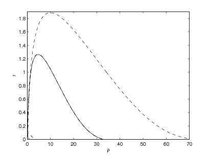
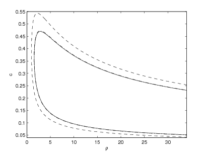
(c)	(d)

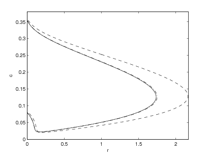
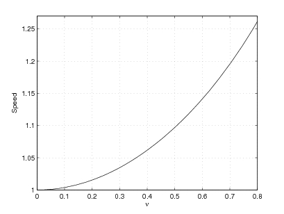
Figure 3: Examples of limit point diagrams for the deterministic and small noise case. In all plots the solid line is $\nu=0$, dot dashed line $\nu=0.1$ and dashed line $\nu=0.5$. Plot (a) is the spine density against the spine stem resistance, plot (b) shows spine density against the speed of the wave and plot (c) shows the spine stem resistance against the speed of the wave. Each plot show an increase in the area of existence in parameter space for the travelling waves as the noise intensity increases. Plot (d) shows the speed of the wave as the noise intensity in the spine head dynamics is increased.

To investigate the effect of the noise on the existence of these waves in parameter space, we choose a point on the fast branch of the deterministic $\rho$-c curve and continue from there in two parameters, for example $\nu_{m}$ (spatially correlated noise intensity in the m-dynamics) and $c$. We can then see how the wave speed changes as noise is added into the equations, Figure 3, plot (d).

3.3 Baer - Rinzel model with variable density, $\rho(x)$

We now look at the speed of a noisy wave as the parameter $\kappa$ changes, and so as the spine stem width changes, for an explanation of the contradictory results from the BR and SDS models with white and OU noise. From the behaviour we have observed so far we expect as $\kappa$ increases and so the model changes from a BR type, $\kappa=0$, to an SDS type, $\kappa=1000$, then the plot of the noisy wave speed should cross the plot of the deterministic wave speed, since the BR model speeds up with the inclusion of noise and we expect the BR model with discrete spine density (as in SDS model) to decrease in speed if the dynamics are not as important as the spine stem morphology. First we consider the new BR model without noise, as the spine stem changes through the increase of parameter $\kappa$.

(a)	(b)

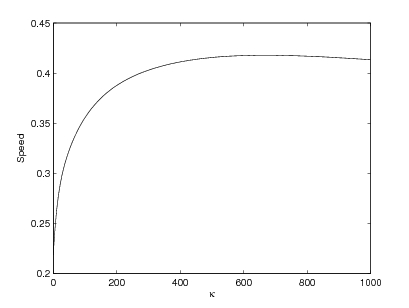
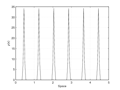
Figure 4: Plot (a) shows the deterministic speed of waves in the modified BR model as the parameter $\kappa$ increases from the BR limit ($\kappa=0$) to the SDS limit ($\kappa\to\infty$). There is an optimal value of $\kappa$ which maximises the speed of the wave, this occurs at $\kappa=670$. Plot (b) shows an examples of the space dependent density. Here $\kappa=670$ and $d=0.8$ is the spine spacing (distance between peaks).

Figure 4, plot (a), shows the speed of a deterministic wave in the modified BR model as $\kappa$ changes and so the spine stem changes from a continuum like the original BR model to a discrete distribution of spines as in the SDS model. There is an optimal value of $\kappa$ which maximises the deterministic wave speed. This shows that the distribution or spine stem morphology is of importance in the propagation of action potentials, it can alter the speed of the AP on the dendrite. Plot (b) shows an example of the spine density for $\kappa=670$. The spatial discretisation will effect the density since a larger $\Delta x$ will approximate a discrete stem at a smaller value of $\kappa$ than a smaller step. The value of speed measured as $\Delta x$ changes is small and the overall behaviour (as $\kappa$ changes) remains the same.

We now consider this variable density BR model with different levels of noise in the spine head dynamics (m-dynamics), in the Itô sense, as $\kappa$ changes. We plot the difference $c_{det}-c_{noisy}$, to show how the noisy wave changes with respect to the deterministic wave as $\kappa$ increases. In order to make it clearer we also show the linear best fit line. It is clear in Figure 5 that the trend is for the wave to be slower ($c_{det}-c_{noisy}>0$) than the deterministic value at the SDS limit (large $\kappa$) and faster ($c_{det}-c_{noisy}<0$) at the BR limit ($\kappa=0$). Figure 5 plot (a) shows the noise intensity at $\nu=0.02$ and plot (b) at $\nu=0.15$.

(a)	(b)

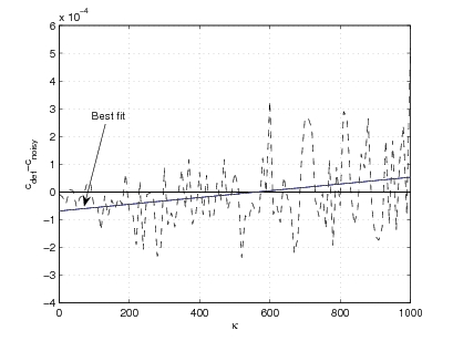
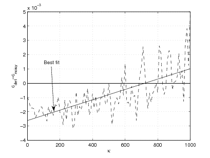
Figure 5: This figure shows the difference between the deterministic speed and the speed of the noisy wave as $\kappa$ increases. The noise is interpreted in the Itô sense. Plot (a) shows $c_{det}-c_{noisy}$, as $\kappa$ increases, where the noise intensity is $\nu=0.02$ and plot (b) has noise intensity $\nu=0.15$. The dotted lines show the difference in the speed, starting negative as the noisy speed is faster than the deterministic wave speed and becoming positive as the noisy wave becomes slower than the deterministic wave. In plot (a) the difference in wave speed is very small but as the noise intensity increases, plot (b), the difference increases and the dotted line is above the line $y=0$ for a larger range of $\kappa$.

It is clear that as the parameter $\kappa$ increases the behaviour of the noisy wave in the new BR model also changes. When $\kappa=0$ the model is the original BR model and the stochastic wave is, on average, faster than the deterministic wave, and as $\kappa$ reaches large values then the wave speed decreases below that of the deterministic wave, mimicking the behaviour of a stochastic wave in the SDS model. This goes to show that the form of the density has an important effect on the behaviour of the model.

4 Additive noise

So far we have only considered multiplicative noise and now briefly show that additive noise in the models can have some interesting effects. When the noise is additive white in the spine heads of both models we can observe synchrony for small levels of noise intensity, see Figure 6.

(a)	(b)

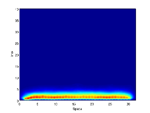
Figure 6: This figure shows the mean voltage in the cable for both the SDS (plot (a)) and BR (plot (b)) model. The colour shows the value of the voltage for each point in space (x-axis) and time (y-axis). As can be seen in both plots the wave is near horizontal which shows that all spines are firing at the same time. Plot (a) shows only one wave due to the long refractory time in the SDS model (which can be controlled by parameter $\tau$) and Plot (b) has many waves due to the natural refractory time of the BR model.

The OU noise (additive and multiplicative) in the m-dynamics of the BR model helps to stabilise waves which were out of order in the white noise case. Figure 7 plots (a) and (b) show the voltage in the cable with additive noise in the m-dynamics, $\mu=0.01$, for white and OU noise respectively. It is clear that the temporal correlation of $\beta=2$ promotes a travelling wave; it could do this by matching some internal time scale in the BR model. Plots (c) and (d) show the voltage in the cable when the noise is multiplicative in the m-dynamics, $\nu=0.1$, for white and $\beta=2$ correlated noise; again the correlation promotes a sequential travelling wave.

(a)	(b)

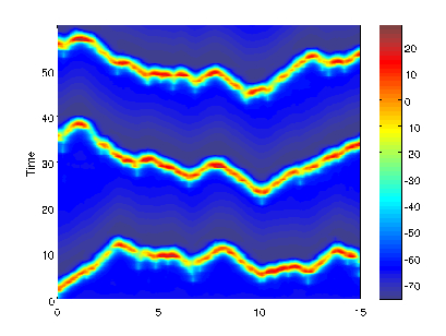
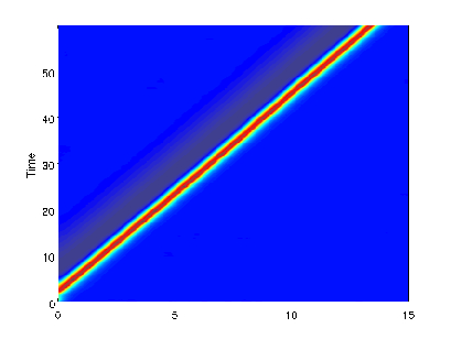
Figure 7: This figure shows a sample of the voltage in the cable when there is noise present in the spine head m-dynamics. Plot (a) has additive white noise of strength $\mu=0.01$, plot (b) has additive OU noise strength $\mu=0.01$ and $\beta=2$. It can be seen that the waves travel out of order when the noise is white but when a temporal correlation is added the waves regain their sequential travel.

The additive spatially correlated noise in the SDS model can stabalise non-sequential travelling waves as the correlation scale increases. Figure 8 shows additive spatially correlated noise in the spines of the SDS model; plot (a) shows the voltage in the cable when the spines are coupled by a short correlation length and the wave fires out of order and plot (b) shows the voltage when the correlation length is longer and this restores the sequential firing of the spines and so the wave travels smoothly again.

(a)	(b)

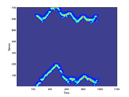
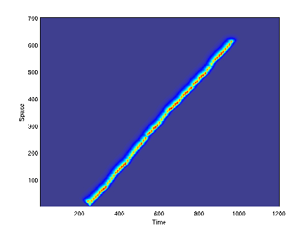
Figure 8: We show here the effect of the correlation length of additive noise in the spine heads of the SDS model for a fixed level of noise intensity. Plot (a) shows a short correlation scale and plot (b) a longer scale and it is clear that the longer correlation scale restores the sequential firing which is lost when the noise has a short correlation length.

The additive spatially correlated noise in the SDS model can stabalise non-sequential travelling waves as the correlation scale increases. Figure 8 shows additive spatially correlated noise in the spines of the SDS model; plot (a) shows the voltage in the cable when the spines are coupled by a short correlation length and the wave fires out of order and plot (b) shows the voltage when the correlation length is longer and this restores the sequential firing of the spines and so the wave travels smoothly again.

5 Discussion

We set out to investigate the effects of different types of noise on models of spiny dendrites and have provided a comparison of white, temporally and spatially correlated noise in the spike-diffuse-spike model and the Baer and Rinzel model. In all cases noise in the cable equation has little effect on the speed of propagation which suggests that the cable is robust whereas the spine dynamics are more sensitive to noisy input. This makes sense with regards to the structure of the models since the cable is passive and diffusive as opposed to the active properties of the spine heads.

When the noise is in the SDS model the speed of any travelling wave decreases as the noise intensity increases but when the noise is in the BR model the speed of travelling waves increases as the noise intensity increases, when the noise is in the spines. The main differences between the two models are the dynamics used to describe the evolution of the spine head voltage (integrate and fire dynamics in the SDS model and the Hodgkin Huxley equations in the BR model) and the spine density, $\rho(x)$ (discretely attached equally spaced spines in the SDS model and a constant in the BR model). This difference could be used to decide which model is a more accurate description of the real dendrite if an experiment could be devised in which the speed of an injected pulse travels the length of a dendrite with noise present. In an attempt to discover which of the differences in the models produced the difference in behaviour we investigated the BR model with a spatially dependent density. In the ’SDS’ limit where the spines are attached discretely the model can be thought to be the SDS model with Hodgkin Huxley dynamics in the spine heads and this model does act like the SDS model when we add noise to the system. Therefore we can conclude that the type of spine dynamics is not the reason for the difference in behaviour between the SDS and BR models and we investigate the affect of the spine density and so the spine stem. As we change the spine density from one limit to the other the cases in between are like looking at spines attached to the cable with a spine stem that has an area of attachment to the cable. The speed of the wave in the deterministic version of this model increases from the BR limit to the SDS limit and there is an optimal value for the spine attachment that gives a maximum value of the speed. When there is noise in the system and we are changing the parameter from BR to SDS limits, the average speed of the wave starts faster than the deterministic wave speed and decreases below the deterministic speed at the SDS limit, in agreement with the previous results from the original SDS and BR models. Although this spatially dependent spine density gives some insight to the importance of the spine stem the model could be improved by a more realistic physical description of the way the spine stems are attached to the cable and perhaps by introducing some random distribution of the spines to investigate how this affects the behaviour. To take this a step further there could even be a simple learning rule introduced which could move the spines in relation to the levels of activity and give a time dependent spine distribution; [32] looks at a simple activity dependent spine plasticity in the BR model, so perhaps this could be extended to include noise. When both models are influenced by spatially correlated noise the interpretation of the noise (Itô or Stratonovich) also changes the behaviour of the travelling waves. The Baer and Rinzel model is not affected when the Itô interpretation is used but the Stratonovich interpretation causes an increase in speed as seen in direct simulation and through a small noise analysis, Section 3.2. Likewise the SDS model shows a change in behaviour: speed reduction in the Itô case and an increase in the Stratonovich case. This begs the question which is the correct noise interpretation for this situation? Is there some way to investigate, experimentally, which is the better noise interpretation for a length of dendrite?

Additive noise in both the dendrite models can induce synchronous behaviour in the spines. For very small levels of noise the systems are fairly robust to the noise; all waves fully propagate and are only subject to a small change in the speed. As the strength of additive noise increases the spines in the models begin to fire out of order and seemingly in a random fashion until a synchronous behaviour takes over and they all fire simultaneously, similarly observed in [22] and [21]. When the noise in the SDS model is additive and spatially correlated in the spine heads then the correlation scale can play a role in restoring sequential firing that has been destroyed by the noise, e.g. when the noise intensity is fixed a short correlation scale displays the out of order firing but as the correlation scale is increased the wave travels in a sequential fashion.

These results suggest that there is an optimal spine density for speed of propagation in dendrites; too sparse and propagation slows down and ultimately stops, too many and we again see a reduction in speed. A spatially correlated noise can also enhance propagation, we used a correlation length of 3 spine spacings which suggests that a localised input to the dendrite, at synapses on neighbouring spines, can increase propagation speed. There are obvious places to extend this work; computationally further investigation of the optimal correlation scale, and propagation of a noisy signal on a dendrite with a random spine distribution. Experimentally it would be useful to verify which noise interpretation is more realistic and if noise speeds up or slows down a real travelling wave.

Table 5 gives the parameter values used throughout this work and their respective units. The values are biologically realistic, and the bracketed values are the non-dimensional values used. The number of spines used in the SDS model was chosen such that they were equally spaced along the (non-dimensional) length of cable used, and such that wave propagation was present.

Symbol	Name	Value	Unit
$V$	Cable Voltage	-	$mV$
$U$	Spine head Voltage	-	$mV$
$R_{m}$	Transmembrane Resistance	2500 (1)	$\Omega cm^{2}$
$R_{a}$	Intracellular Resistance	70 (1)	$\Omega cm$
$C_{m}$	Transmembrane Capacitance	1 (1)	$\mu Fcm^{-2}$
$\hat{C}$	Transmembrane Capacitance of Spine head	1 (1)	$\mu Fcm^{-2}$
$\hat{r}$	Transmemrane Resistance of Spine head	2500 (1)	$\Omega cm^{2}$
$\mu$	Strength of additive noise	-	-
$\nu$	Strength of multiplicative noise	-	-
$a$	Dendritic Diameter	0.36 (1)	$\mu m$
$\lambda=\sqrt{aR_{m}}{4R_{a}}$	Electronic Length Scale	(1)	-
$\tau=R_{m}C_{m}$	Electonic time constant	(1)	-
$D=\frac{\lambda^{2}}{\tau}$	Diffusion Coefficient	(1)	-
$\tau_{R}$	Refractory time	-	-
$L$	Length of dendrite	1-2	$mm$
$N_{spines}$	Number of spines in SDS model	81	-
$\tau_{s}$	Length of time pulse lasts in SDS model	-	-
$h$	Voltage threshold in spine head for SDS model	0.04	-
$m$	Sodium activation particle	-	-
$h$	Sodium inactivation particle	-	-
$n$	Potassium activation particle	-	-
$G_{Na}$	Maximum sodium conductance	120	$mScm^{-2}$
$G_{K}$	Maximum potassium conductance	36	$mScm^{-2}$
$G_{L}$	Maximum leakage conductance	0.3	$mScm^{-2}$
$V_{Na}$	Sodium reversal potential	50	$mV$
$V_{K}$	Potassium reversal potential	-77	$mV$
$V_{L}$	Leakage reversal potential	-54.402	$mV$
$\rho$	Spine density	-	-
$d$	Spine spacing	(0.8 or 1)	$\mu m$
$\eta_{0}$	Strength of action potential (AP) pulse in SDS model	-	-

References

- [1] P. Andersen, R. Morris, D. Amaral, T. Bliss, and J. O’Keefe. The Hippocampus book. Oxford University Press, 2007.
- [2] S. M. Baer and J. Rinzel. Propagation of dendritic spikes mediated by excitable spines: A continuum theory. Journal of Neurophysiology, 65(4):874–890, 1991.
- [3] T. Bonhoeffer and R. Yuste. Spine motility: phenomenology, mechanisms and function. Neuron, 35:1019 – 1027, 2002.
- [4] S. Coombes and P. C. Bressloff. Solitary waves in a model of dendritic cable with active spines. SIAM Journal on Applied Mathematics, 61:432–453, 2000.
- [5] S. Coombes and P. C. Bressloff. Saltatory waves in the spike-diffuse-spike model of active dendritic spines. Physical Review Letters, 91, 2003.
- [6] E. J. Coutts. The effect of noise in models of spiny dendrites. PhD thesis, Heriot Watt University, May 2010.
- [7] Y. Dan and M. Poo. Spike timing dependent plasticity of neural circuits. Neuron, 44:23 – 30, 2004.
- [8] E. Doedel, A. R. Champneys, T. R. Fairgrieve, Y. A. Kuznetsov, B. Sandstede, and X. J. Wang. AUTO-07P. http://indy.cs.concordia.ca/auto, 1997.
- [9] C. R. Doering, K. V. Sargsyan, and P. Smereka. A numerical method for some stochastic differential equations with multiplicative noise. Physics Letters A, 344:149–155, 2005.
- [10] A. A. Faisal, L. P. J. Selen, and D. M. Wolpert. Noise in the nervous system. Nature reviews neuroscience, 9:292–303, 2008.
- [11] J. García-Ojalvo and J. M. Sancho. Noise in spatially extended systems. Springer, 1999.
- [12] C. W. Gardiner. Handbook of stochastic methods: for physics, chemistry and the natural sciences. Springer-Verlag, 1983.
- [13] W. Gerstner and W. M. Kistler. Spiking neuron models: Single neurons, populations, plasticity. Cambridge University Press, 2002.
- [14] M. Haüsser, N. Spruston, and G. J. Stuart. Diversity and dynamics of dendritic signalling. Science, 290, 2000.
- [15] H. Kasai. Structure stability function relationships of dendritic spines. Trends in neuroscience, 26(7), 2003.
- [16] P. E. Kloeden and E. Platen. Numerical solution of stochastic differential equations. Springer-Verlag, 1992.
- [17] B. Lindner, A. Longtin, and A. Bulsara. Analytic expressions for rate and CV of a type I neuron driven by white gaussian noise. Neural computation, 15:1761 – 1788, 2003.
- [18] G. J. Lord and S. Coombes. Traveling waves in the Baer and Rinzel model of spine studded dendritic tissue. Physica D, 161:1 – 20, 2002.
- [19] A. Manwani and C. Koch. Detecting and estimating signals in noisy cable structures, i: Neuronal noise sources. Neural Computation, 11:1797–1829, 1999.
- [20] B. W. Mel. Information processing in dendritic trees. Neural computation, 6, 1994.
- [21] K. A. Newhall, G. Kovacic, P. R. Kramer, and D. Cai. Cascade-induced synchrony in stochastically-driven neuronal networks. Physical review E, To Appear.
- [22] K. A. Newhall, G. Kovacic, P. R. Kramer, D. Zhou, A. V. Rangan, and D. Cai. Dynamics of current-based poisson driven integrate-and-fire neuronal networks. Communication Math Science, 2010.
- [23] B. Øksendal. Stochastic differential equations: An introduction with applications. Springer, 2007.
- [24] A. Roth P. Vetter and M. Haüsser. Propagation of action potentials in dendrites depends on dendritic morphology. Journal of Neurophysiology, 85:926–937, 2001.
- [25] M. Rudolph and A. Destexhe. A fast conducting stochastic integrative mode for neocortical neurons in vivo. Journal of Neuroscience, 23:2466–2476, 2003.
- [26] A. Scott. Neuroscience: A mathematical primer. Springer-Verlag, 2002.
- [27] I. Segev and W. Rall. Excitable dendrites and spines: Earlier theoretical insights elucidate recent direct observations. TINS, 21:453–460, 1998.
- [28] T. Shardlow. Numerical simulation of stochastic PDEs for excitable media. Journal of computational and applied mathematics, 175:429–446, 2005.
- [29] R. F. Thompson. The Brain: An introduction to neuroscience. W H Freeman and Company, 1985.
- [30] Y. Timofeeva, G. J. Lord, and S. Coombes. Spatio-temporal filtering properties of a dendritic cable with active spines: A modelling study in the spike-diffuse-spike framework. Journal of Computational Neuroscience, 2006.
- [31] P. S. Ulinski, E. G. Jones, and A. Peters. Cerebral cortex. Kluwer Academic, 1999.
- [32] D.W. Verzi, M.B. Rheuben, and S.M. Baer. Impact of time dependent changes in spine density and spine shape on the input-output properties of a dendritic branch: a computational study. Journal of neurophysiology, 93:2073 – 2089, 2005.
- [33] R. Yuste and W. Denk. Dendritic spines as a basic functional units of neuronal integration. Nature, 375:682–684, 1995.