Within the effective mass approximation an adiabatic description of spheroidal and dumbbell quantum dot models in the regime of strong dimensional quantization is presented using the expansion of the wave function in appropriate sets of single-parameter basis functions. The comparison is given and the peculiarities are considered for spectral and optical characteristics of the models with axially symmetric confining potentials depending on their geometric size making use of the total sets of exact and adiabatic quantum numbers in appropriate analytic approximations.

Key words: spheroidal and dumbbell quantum dot models, boundary-value problem, Kantorovich method, adiabatic approximation, absorption coefficient

Blessed memory of professor Sissakian Alexei Norairovich is devoted

1 Introduction

To analyze the geometrical, spectral and optical characteristics of quantum dots in the effective mass approximation and in the regime of strong dimensional quantization following  [1], many methods and models were used. We mention some of them, that are in the field of our interest: the exactly solvable models of spherical and cylindrical layer (toroid) impermeable wells  [2, 3], the adiabatic approximation for a lens-shaped well confined to a narrow wetting layer [4], and a hemispherical impermeable well [5], the model of strongly oblate or prolate ellipsoidal impermeable well  [6, 7, 8], as well as numerical solutions of the boundary value problems (BVPs) with separable variables in the spheroidal coordinates for wells with infinite and finite wall heights  [9, 10, 11, 12, 13], Möbius [14] nanostructures, scattering problems for toric  [15] and coupled nonidentical microdisks  [16].

Similar models were used for describing the energy spectra of deformed nuclei [17, 18, 19, 20, 21, 22, 23], atomic clusters deposited on planar surfaces [24] and low-energy barrier nuclear reactions [25, 27, 28, 29, 30]. However, thorough comparative analysis of spectral and optical characteristics of models with different potentials, including those with non-separable variables, remains to be a challenging problem.

In the present paper we analyze the spectral and optical characteristics of the following models: a spherical quantum dot (SQD), an oblate spheroidal quantum dot (OSQD), a prolate spheroidal quantum dot (PSQD), and a dumbbell QDs (DQD). We make use of the Kantorovich method that reduces the problem to a set of ordinary differential equations (ODE) [31] by means of the expansion of the wave function in appropriate sets of single-parameter basis functions [32] similar to the well-known adiabatic method [33].

We present briefly a calculation scheme for solving elliptical BVPs with axially-symmetric potentials in cylindrical coordinates (CC), spherical coordinates (SC), oblate spheroidal coordinates (OSC), and prolate spheroidal coordinates (PSC). Basing on the symbolic-numerical algorithms (SNA) developed for axially-symmetric potentials [34, 35, 36], different sets of solutions are constructed for the parametric BVPs related to the fast subsystem, namely, the eigenvalue problem solutions (the terms and the basis functions), depending upon the slow variable as a parameter, as well as the matrix elements, i.e., the integrals of the products of basis functions and their derivatives with respect to the parameter. These terms and matrix elements form the matrices of variable coefficients in the set of second-order ODE with respect to the slow variable, which are calculated in special cases analytically and in the general case using the program ODPEVP [37]. The BVP for this set of ODEs is solved by means of the program KANTBP [38], while in the special cases crude diagonal estimations can be performed using the appropriate analytic approximations.

The efficiency of the calculation scheme and the SNA used is demonstrated by tracing the peculiarities of spectral and optical characteristics in the course of varying the ellipticity of the prolate or oblate spheroid and dumbbell in the models of quantum dots with different confining potentials, such as the isotropic and anisotropic harmonic oscillator, the spherical and spheroidal well with finite or infinite walls approximated by smooth short-range potentials, as well as by constructing the adiabatic classification of the states.

The paper is organized as follows. In Section 2, the calculation scheme for solving elliptic BVPs with axially-symmetric confining potentials is briefly presented. Sections 3 and 4 are devoted to the analysis of the spectra and absorption coefficient of quantum dot models with three types of axially-symmetric potentials, including the benchmark exactly solvable models. In Conclusion we summarize the results and discuss the future applications.

2 Problem Statement

Within the effective mass approximation under the conditions of strong dimensional quantization, the Schrödinger equation for the slow envelope of the wave function $\tilde{\Psi}(\tilde{\vec{r}})$ of a charge carrier (electron $e$ or hole $h$) in the models of QDs has the form [6, 7]

$$\{\tilde{\hat{H}}-\tilde{E}\}\tilde{\Psi}(\tilde{\vec{r}})=\{({2\mu_{p}})^{-1}\tilde{\hat{{\vec{P}}}}^{2}+\tilde{U}(\tilde{\vec{r}})-\tilde{E}\}\tilde{\Psi}(\tilde{\vec{r}})=0,$$ (1)

where $\tilde{\vec{r}}\in\bf R^{3}$ is the position vector of the particle having the effective mass $\mu_{p}=\mu_{e}$ (or $\mu_{p}=\mu_{h}$), $\tilde{\hat{{\vec{P}}}}=-i\hbar\nabla_{\tilde{\vec{r}}}$ is the momentum operator, $\tilde{E}$ is the energy of the particle, $\tilde{U}(\tilde{\vec{r}})$ is the axially-symmetric potential confining the particle motion in SQD, PSQD, or OSQD. In Model A, $\tilde{U}(\tilde{\vec{r}})$ is chosen to be the potential of an isotropic or anisotropic axially-symmetric harmonic oscillator in Cartesian coordinates ${\vec{r}=\{x,y,z\}}$:

$$\tilde{U}^{\mbox{A}}(\tilde{\vec{r}})={\mu_{p}\tilde{\omega}^{2}(\zeta_{1}(\tilde{x}^{2}+\tilde{y}^{2})+\zeta_{3}\tilde{z}^{2})}/{2}.$$ (2)

Here $\zeta_{1}=1$, $\zeta_{3}=1$ for a spherical QD or $\zeta_{1}=(\tilde{r}_{0}/\tilde{a})^{4}$, $\zeta_{3}=(\tilde{r}_{0}/\tilde{c})^{4}$ for a spheroidal QD, inscribed into a spherical one, where $\tilde{a}$ and $\tilde{c}$ are the semiaxes of the ellipse which transforms into a sphere at $\tilde{a}=\tilde{c}=\tilde{r}_{0}=\sqrt{\tilde{x}_{0}^{2}+\tilde{y}_{0}^{2}+\tilde{z}_{0}^{2}}$, $\tilde{\omega}=\gamma_{\tilde{r}_{0}}{\hbar}/({\mu_{p}\tilde{r}_{0}^{2}})$ is the angular frequency, and $\gamma_{\tilde{r}_{0}}$ is an adjustable parameter. We will use the value $\gamma_{\tilde{r}_{0}}=\pi^{2}/3$ that follows from equating the ground state energies for the spherical oscillator and the spherical QD of Model B considered below. If necessary, this definition can be replaced with a different one, e.g., the one conventional for nuclear physics [21, 22, 23].

For Model B, $\tilde{U}(\tilde{\vec{r}})$ is the potential of a spherical or axially-symmetric well

$$\tilde{U}^{\mbox{B}}(\tilde{\vec{r}})=\{0,S(\tilde{\vec{r}})<0;\tilde{U}_{0},S(\tilde{\vec{r}})\geq 0\},$$ (3)

bounded by the surface $S(\tilde{\vec{r}})=0$ with walls of finite or infinite height $1\ll\tilde{U}_{0}<\infty$. In Eq. (3) $S(\tilde{\vec{r}})$ depends on the parameters $\tilde{a}$, $\tilde{c}$, and $0\leq\tilde{c}_{1}\leq 1$

$$S(\tilde{\vec{r}})\equiv\frac{\tilde{x}^{2}+\tilde{y}^{2}}{\tilde{a}^{2}}+\frac{(\tilde{z}^{2}-\tilde{c}^{2})(\tilde{z}^{2}\tilde{c}_{1}^{2}+1-\tilde{c}_{1}^{2})^{2}}{\tilde{c}^{2}(\tilde{c}_{1}^{2}\tilde{c}^{2}/4+1-\tilde{c}_{1}^{2})^{2}}$$ (4)

At $c_{1}=0$ we get a spheroidal quantum dot model, at $0<c_{1}<1$ it becomes a dumbbell QD with a symmetric double well, and at $c_{1}>1$ we get a triple-well model.

For Model C, $\tilde{U}(\tilde{\vec{r}})$ is taken to be a spherical or axially-symmetric diffuse potential

$$\tilde{U}^{\mbox{C}}(\tilde{\vec{r}})=\tilde{U}_{0}\left(1-\left(1+\exp(S(\tilde{\vec{r}})/{s})\right)^{-1}\right),$$ (5)

where $s$ is the edge diffusiveness parameter of the function smoothly approximating the vertical walls of finite height $\tilde{U}_{0}$. Below we restrict ourselves by considering Model B with infinite walls $\tilde{U}_{0}\rightarrow\infty$ and Model C with walls of finite height $\tilde{U}_{0}$.

Throughout the paper we make use of the reduced atomic units [1, 7]: $a_{B}^{*}={\kappa\hbar^{2}}/{\mu_{p}e^{2}}$ is the reduced Bohr radius, $\kappa$ is the DC permittivity, $\tilde{E}_{R}\equiv Ry^{*}={\hbar^{2}}/({2\mu_{p}{a_{B}^{*}}^{2}})$ is the reduced Rydberg unit of energy, and the following dimensionless quantities are introduced: $\tilde{\Psi}(\tilde{\vec{r}})={a_{B}^{*}}^{-3/2}\Psi({\vec{r}})$, $2{\hat{H}}=\tilde{\hat{H}}/{Ry^{*}}$, $2{E}={\tilde{E}}/{Ry^{*}}$, $2{U(\vec{r})}={\tilde{U}(\tilde{\vec{r}})}/{Ry^{*}}$, $\vec{r}=\tilde{\vec{r}}/a_{B}^{*}$, $a=\tilde{a}/a_{B}^{*}$, $\tilde{c}=c/a_{B}^{*}$,$\tilde{c}_{1}=c_{1}/a_{B}^{*}$, $r_{0}=\tilde{r}_{0}/a_{B}^{*}$, $\omega=\gamma_{r_{0}}/r_{0}^{2}=\hbar\tilde{\omega}/(2Ry^{*})$. For an electron with the effective mass $\mu_{p}\equiv\mu_{e}=0.067m_{0}$ at $\kappa=13.18$ in GaAs: $a_{B}^{*}=a_{B}^{e}=104\;{}^{{}^{o}}\!\!\!\!A=10.4$ nm and $Ry^{*}=\tilde{E}^{e}_{R}=5.275$ meV. For a heavy hole with the effective mass $\mu_{h}=\mu_{e}/0.12=0.558m_{0}$ the corresponding values are $a_{B}^{h}=a_{B}^{e}(\mu_{e}/\mu_{h})=12.48\;{}^{{}^{o}}\!\!\!\!A=1.248$ nm, and $\tilde{E}^{h}_{R}=\tilde{E}^{e}_{R}(\mu_{h}/\mu_{e})=46.14$ meV.

Note, that for model A of approximation of OSQD/PSQD by the anisotropic oscillator (2) the separation of variables in cylindric coordinates $\vec{x}=(z,\rho,\varphi)$ is possible and additional integrals exist [39, 40, 41]. Similarly, for model B the variables are separable in the oblate/prolate spheroidal coordinates $\vec{x}=(\xi,\eta,\varphi)$ and the additional integrals of motion are $\hat{\Lambda}$: $[\hat{H},\hat{\Lambda}]\equiv\hat{H}\hat{\Lambda}-\hat{\Lambda}\hat{H}=0$, i.e. $\hat{H}_{p}$ and $\hat{\Lambda}_{p}$ in PSQD

$$\hat{H}_{p}=-\frac{4}{d^{2}}\left[\frac{1}{\xi^{2}-\eta^{2}}\left(\frac{d}{d\xi}(\xi^{2}-1)\frac{d}{d\xi}+\frac{d}{d\eta}(1-\eta^{2})\frac{d}{d\eta}\right)+\biggl{(}\frac{1}{(\xi^{2}-1)(1-\eta^{2})}\biggr{)}\frac{d^{2}}{d\varphi^{2}}\right],$$ (6)

$$\hat{\Lambda}_{p}=\frac{1-\eta^{2}}{\xi^{2}-\eta^{2}}\frac{d}{d\xi}(\xi^{2}-1)\frac{d}{d\xi}+\frac{\xi^{2}-1}{\xi^{2}-\eta^{2}}\frac{d}{d\eta}(1-\eta^{2})\frac{d}{d\eta}+\biggl{(}\frac{1}{\xi^{2}-1}-\frac{1}{1-\eta^{2}}\biggr{)}\frac{d^{2}}{d\varphi^{2}},$$ (7)

$\hat{H}_{o}$ and $\hat{\Lambda}_{o}$ in OSQD

$$\hat{H}_{o}=-\frac{4}{d^{2}}\left[\frac{1}{\xi^{2}+\eta^{2}}\left(\frac{d}{d\xi}(\xi^{2}+1)\frac{d}{d\xi}+\frac{d}{d\eta}(1-\eta^{2})\frac{d}{d\eta}\right)-\biggl{(}\frac{1}{(\xi^{2}+1)(1-\eta^{2})}\biggr{)}\frac{d^{2}}{d\varphi^{2}}\right],$$ (8)

$$\hat{\Lambda}_{o}=-\frac{1-\eta^{2}}{\xi^{2}+\eta^{2}}\frac{d}{d\xi}(\xi^{2}+1)\frac{d}{d\xi}-\frac{\xi^{2}+1}{\xi^{2}+\eta^{2}}\frac{d}{d\eta}(1-\eta^{2})\frac{d}{d\eta}-\biggl{(}\frac{1}{\xi^{2}+1}+\frac{1}{1-\eta^{2}}\biggr{)}\frac{d^{2}}{d\varphi^{2}}.$$ (9)

Eq. (9) is obtained by substituting $\xi\rightarrow\imath\xi$, $d\rightarrow-\imath d$ from the known (7) derived in [42, 43].

Since the Hamiltonian $\hat{H}$ in Eqs. (1)–(5) commutes with the $z$-parity operator of reflection in the plane $z=0$ ($z\to-z$ or $\eta\to-\eta$), the solutions are divided into even ($\sigma=+1$) and odd ($\sigma=-1$) ones. The solution of Eq. (1), periodical with respect to the azimuthal angle $\varphi$, is sought in the form of a product $\Psi(x_{f},x_{s},\varphi)=\Psi^{m\sigma}(x_{f},x_{s}){e^{im\varphi}}/{\sqrt{2\pi}}$, where $m=0,\pm 1,\pm 2,...$ is the magnetic quantum number. Note, in absence of magnetic fields the Hamiltonian commutes also with the inversion operator ($\vec{r}\to-\vec{r}$) with eigenvalues $\hat{\sigma}=(-1)^{m}\sigma$ and solution divided into gerade ($\hat{\sigma}=+1$) and ungerade ($\hat{\sigma}=-1$) ones. Then the function $\Psi^{m\sigma}(x_{f},x_{s})$ satisfies the following equation in the two-dimensional domain $\Omega=\Omega_{x_{f}}(x_{s})\cup\Omega_{x_{s}}\subset{\bf R}^{2}\backslash\{0\}$, $\Omega_{x_{f}}(x_{s})=(x_{f}^{\min}(x_{s}),x_{f}^{\max}(x_{s}))$, $\Omega_{x_{s}}=(x_{s}^{\min},x_{s}^{\max})$:

$$\left(\hat{H}_{1}(x_{f};x_{s})+\hat{H}_{2}(x_{s})+V(x_{f},x_{s})-2{E}\right)\Psi^{m\sigma}(x_{f},x_{s})=0.$$ (10)

The Hamiltonian of the slow subsystem $\hat{H}_{2}(x_{s})$ is expressed as

$$\hat{H}_{2}(x_{s})=\check{H}_{2}(x_{s})=-\frac{1}{g_{1s}(x_{s})}\frac{\partial}{\partial x_{s}}g_{2s}(x_{s})\frac{\partial}{\partial x_{s}}+\check{V}_{s}(x_{s}),$$ (11)

and the Hamiltonian of the fast subsystem $\hat{H}_{1}(x_{f};x_{s})$ is expressed in terms of the reduced Hamiltonian $\check{H}_{f}(x_{f};x_{s})$ and the weighting factor $g_{3s}(x_{s})$:

$$\hat{H}_{1}(x_{f};x_{s})=g_{3s}^{-1}(x_{s})\check{H}_{f}(x_{f};x_{s}),$$ (12)

$$\check{H}_{f}(x_{f};x_{s})=-\frac{1}{g_{1f}(x_{f})}\frac{\partial}{\partial x_{f}}g_{2f}(x_{f})\frac{\partial}{\partial x_{f}}+\check{V}_{f}(x_{f})+\check{V}_{fs}(x_{f},x_{s}).$$

Table 1: The values of conditionally fast $x_{f}$ and slow $x_{s}$ independent variables, the coefficients $g_{is}(x_{s})$, $g_{jf}(x_{f})$ and the potentials $\check{V}_{f}(x_{f})$, $\check{V}_{s}(x_{s})$, $\check{V}_{fs}(x_{f},x_{s})$, in Eqs.(10)–(12) for SQD, OSQD and PSQD in cylindrical (CC), spherical (SC) and oblate $\&$ prolate spheroidal (OSC $\&$ PSC) coordinates with $(d/2)^{2}=\pm(a^{2}-c^{2})$, $+$ for OSC, $-$ for PSC.

	CC		SC	OSC $\&$PSC
	OSQD	PSQD	SQD	OSQD $\&$ PSQD
$x_{f}$	$z$	$\rho$	$\eta$	$\eta$
$x_{s}$	$\rho$	$z$	$r$	$\xi$
$g_{1f}$	$1$	$\rho$	$1$	$1$
$g_{2f}$	$1$	$\rho$	$1-\eta^{2}$	$1-\eta^{2}$
$g_{1s}$	$\rho$	$1$	$r^{2}$	$1$
$g_{2s}$	$\rho$	$1$	$r^{2}$	$\xi^{2}\pm 1$
$g_{3s}$	$1$	$1$	$r^{2}$	$1$
${\check{V}}_{f}(x_{f})$	$\omega^{2}\zeta_{3}z^{2}$	$m^{2}/\rho^{2}+\omega^{2}\zeta_{1}\rho^{2}$	$m^{2}/g_{2f}$	$m^{2}/g_{2f}\pm(d/2)^{2}g_{2f}2E$
${\check{V}}_{s}(x_{s})$	$m^{2}/\rho^{2}+\omega^{2}\zeta_{1}\rho^{2}$	$\omega^{2}\zeta_{3}z^{2}$	$0$	$\mp m^{2}/g_{2s}-((d/2)^{2}g_{2s}-1)2E$
${\check{V}}_{fs}(x_{f},x_{s})$	$0$	$0$	${\check{V}}(r,\eta)$	${\check{V}}(\xi,\eta)$

Table 1 contains a detailed description of the conditionally fast $x_{f}$ and slow $x_{s}$ independent variables, the coefficients $g_{1s}(x_{s})$, $g_{2s}(x_{s})$, $g_{3s}(x_{s})$, $g_{1f}(x_{f})$, $g_{2f}(x_{f})$, and the reduced potentials $\check{V}_{f}(x_{f})$, $\check{V}_{s}(x_{s})$, $\check{V}_{fs}(x_{f},x_{s})$, entering Eqs. (10)–(12) for SQD, OSQD, and PSQD in cylindrical ($\vec{x}=(z,\rho,\varphi)$), spherical ($\vec{x}=(r,\eta=\cos\theta,\varphi)$), and oblate/prolate spheroidal ($\vec{x}=(\xi,\eta,\varphi)$) coordinates (CS, SC and OSC/PSC) [44]. Note, that in Table 1, using Eqs. (2), (5) in the reduced atomic units, the potential $\check{V}(r,\eta)$ for OSQD/PSQD in SC is expressed for Model A as

$$\check{V}(r,\eta)={2}r^{2}U^{A}(r,\eta)={\omega^{2}r^{4}(\zeta_{1}(1-\eta^{2})+\zeta_{3}\eta^{2})},$$

and for Model C as

$$\check{V}(r,\eta)={2}r^{2}U^{C}(r,\eta)={2}r^{2}U_{0}\left(1-\left(1+\exp(({r^{2}(\frac{(1-\eta^{2})}{a^{2}}+\frac{\eta^{2}}{c^{2}})-1})/{s})\right)^{-1}\right),$$

both having zero normal first derivatives $\partial V(r,\eta)/\partial r$ in the vicinity of the origin $r=0$ (equilibrium point), similar to [26]. We do not use the CC for Model C, because the motion in this case is not restricted by two coordinates $\rho$ and $z$. For Model B in Table 1 $\omega=0$ and the potentials ${\check{V}}(r,\eta)={\check{V}}(\xi,\eta)=0$ are zero, since in this case one should impose the Dirichlet boundary conditions $\Psi^{m\sigma}(x_{f},x_{s})|_{\partial\Omega}=0$ at the boundary $\partial\Omega=\{{\cal R}^{2}|S(x_{f},x_{s})=0\}$ of $\Omega$ restricted by the surface $S(\tilde{\vec{r}})=0$, which is equivalent to the action of the potential (3).

The solution $\Psi^{m\sigma}_{i}(x_{f},x_{s})\equiv\Psi^{Em\sigma}_{i}(x_{f},x_{s})$ of the problem (10)–(12) is sought in the form of Kantorovich expansion [31]

$$\Psi^{Em\sigma}_{i}(x_{f},x_{s})=\sum_{j=1}^{j_{\max}}\Phi^{m\sigma}_{j}(x_{f};x_{s})\chi_{j}^{(m\sigma i)}(E,x_{s}).$$ (13)

The set of appropriate trial functions is chosen as the set of eigenfunctions $\Phi^{m\sigma}_{j}(x_{f};x_{s})$ of the Hamiltonian $\check{H}_{f}(x_{f};x_{s})$ from (12), i.e., the solutions of the parametric BVP

$$\left\{\check{H}_{f}(x_{f};x_{s})-\check{\lambda}_{i}(x_{s})\right\}\Phi_{i}^{m\sigma}(x_{f};x_{s})=0,$$ (14)

in the interval $x_{f}\in\Omega_{x_{f}}(x_{s})$, depending on the conditionally slow variable $x_{s}\in\Omega_{x_{s}}$ as on a parameter. These solutions obey the boundary conditions

$$\lim\limits_{x_{f}\to x_{f}^{t}(x_{s})}\!\!\left(\!\!{N_{f}^{(m\sigma)}(x_{s})g_{2f}(x_{f})\frac{d\Phi_{j}^{m\sigma}(x_{f};x_{s})}{dx_{f}}+D_{f}^{(m\sigma)}(x_{s})\Phi_{j}^{m\sigma}(x_{f};x_{s})}\!\!\right)\!\!=\!\!0$$ (15)

at the boundary points $\{x_{f}^{\min}(x_{s}),x_{f}^{\max}(x_{s})\}=\partial\Omega_{x_{f}}(x_{s})$, of the interval $\Omega_{x_{f}}(x_{s})$. In Eq. (15), $N_{f}^{(m\sigma)}(x_{s})\equiv N_{f}^{(m\sigma)}$, $D_{f}^{(m\sigma)}(x_{s})\equiv D_{f}^{(m\sigma)}$, unless specially declared, are determined by the relations $N_{f}^{(m\sigma)}=1$, $D_{f}^{(m\sigma)}=0$ at $m=0$, $\sigma=+1$ (or at $\sigma=0$, i.e., without parity separation), $N_{f}^{(m\sigma)}=0$, $D_{f}^{(m\sigma)}=1$ at $m=0$, $\sigma=-1$ or at $m\neq 0$. The eigenfunctions satisfy the orthonormality condition with the weighting function $g_{1f}(x_{f})$ in the same interval $x_{f}\in\Omega_{x_{f}}(x_{s})$:

$$\left\langle\Phi_{i}^{m\sigma}|\Phi_{j}^{m\sigma}\right\rangle=\int\nolimits_{x_{f}^{\min}(x_{s})}^{x_{f}^{\max}(x_{s})}\Phi_{i}^{m\sigma}(x_{f};x_{s})\Phi_{j}^{m\sigma}(x_{f};x_{s})g_{1f}(x_{f})dx_{f}=\delta_{ij}.$$ (16)

Here $\check{\lambda}_{1}(x_{s})<...<\check{\lambda}_{j_{\max}}(x_{s})<...$ is the desired set of real eigenvalues. The corresponding set of potential curves $2{E}_{1}(x_{s})<...<2{E}_{j_{\max}}(x_{s})<...$ of Eqs. (12) is determined by $2{E}_{j}(x_{s})=g_{3s}^{-1}(x_{s})\check{\lambda}_{j}(x_{s})$. Note that for OSC and PSC, the desired set of real eigenvalues $\check{\lambda}_{j}(x_{s})$ depends on the combined parameter, $x_{s}\rightarrow p^{2}=(d/2)^{2}2E$, i.e., the product of spectral $2E$ and geometrical $(d/2)^{2}$ parameters of the problem (10). The solutions of the problem (14)–(16) for Models A and B are calculated in the analytical form [36], while for Model C this is done using the program ODPEVP [37]. Substituting the expansion (13) into Eq. (1), we get a set of ODEs for the slow subsystem with respect to the unknown vector functions ${\mbox{\boldmath$\chi$}}^{(m\sigma i)}(x_{s},E)\equiv{\mbox{\boldmath$\chi$}}^{(t)}(x_{s})=(\chi_{1}^{(t)}(x_{s}),...,\chi_{j_{\max}}^{(t)}(x_{s}))^{T}$:

$$\!\!\!\!\!\!\biggl{(}\!-\!\frac{1}{g_{1s}(x_{s})}\frac{d}{d{x_{s}}}g_{2s}(x_{s})\frac{d}{d{x_{s}}}+\check{V}_{s}(x_{s})+{V}_{ii}(x_{s})-2{E}\biggr{)}\chi_{i}^{(t)}({x_{s}})=\!-\!\sum_{j}{V}_{ij}(x_{s})\chi_{j}^{(t)}({x_{s}}).$$ (17)

Here $V_{ii}(x_{s})=2E_{i}(x_{s})+H_{ii}(x_{s})$, ${V}_{ij}(x_{s})$ are defined by formula

$${V}_{ij}(x_{s})=\frac{g_{2s}(x_{s})}{g_{1s}(x_{s})}H_{ij}({x_{s}})+\frac{1}{g_{1s}(x_{s})}\frac{dg_{2s}(x_{s})Q_{ij}({x_{s}})}{d{x_{s}}}\!+\!\frac{g_{2s}(x_{s})}{g_{1s}(x_{s})}Q_{ij}({x_{s}})\frac{d}{dx_{s}},$$

$$H_{ij}(x_{s})=H_{ji}(x_{s})=\int\nolimits_{x_{f}^{\min}(x_{s})}^{x_{f}^{\max}(x_{s})}g_{1f}(x_{f})\frac{\partial\Phi_{i}(x_{f};x_{s})}{\partial x_{s}}\frac{\partial\Phi_{j}(x_{f};x_{s})}{\partial x_{s}}dx_{f},$$ (18)

$$Q_{ij}(x_{s})=-Q_{ji}(x_{s})=-\int\nolimits_{x_{f}^{\min}(x_{s})}^{x_{f}^{\max}(x_{s})}g_{1f}(x_{f})\Phi_{i}(x_{f};x_{s})\frac{\partial\Phi_{j}(x_{f};x_{s})}{\partial x_{s}}dx_{f},$$

and calculated analytically for Model B and by means of the program ODPEVP [37] for Model C, while the solutions of the BVPs for Eqs. (17) with the boundary and orthonormalization conditions of the type (15), (16) with $x_{f}\rightarrow x_{s}$ were calculated by means of the program KANTBP [38]. Note, that for Model A in SC or CC and Model B in OSC or PSC, the variables $x_{f}$ and $x_{s}$ are separated so that the matrix elements $\check{V}_{ij}(x_{s})0$ are put into the r.h.s. of Eq. (17), and $V_{s}(x_{s})$ are substituted from Table 1. For the interesting lower part of the spectrum of Models A and B $2E:2E_{1}<2E_{2}<\ldots<2E_{t}$, or of Model C $2E:2E_{1}<2E_{2}<\ldots<2E_{t}<2U_{0}$, the number $j_{\max}$ of the equations solved should be at least not less than the number of the energy levels of the problem (17) at $a=c=r_{0}$. To ensure the prescribed accuracy of calculation of the lower part of the spectrum discussed below with eight significant digits we used $j_{\max}=16$ basis functions in the expansion (8) and the discrete approximation of the desired solution by Lagrange finite elements of the fourth order with respect to the grid pitch $\Omega^{p}_{h^{s}(x_{s})}=[x_{s;\min},x_{s;k}=x_{s;k-1}+h_{s},x_{s;\max}]$. The details of the corresponding computational scheme are given in [36].

3 Spectral Characteristics of Spheroidal
and Dumbbell QDs

3.1 Model A of OSQD & PSQD

In the exactly solvable model A the variables are separable in spherical coordinates, and under the variation of the aspect ratio parameters $\zeta_{ca}=c/a$ and $\zeta_{ac}=\zeta_{ca}^{-1}=a/c$ for the oblate and prolate spheroids, determining the transverse $\omega_{\rho}=\sqrt{\zeta}_{1}\omega$ and longitudinal $\omega_{z}=\sqrt{\zeta}_{3}\omega$ frequencies of the circular and linear harmonic oscillators. The spectrum is given by the sum of energies $2E_{n_{\rho}m}=2\omega_{\rho}(2n_{\rho}+|m|+1),n_{\rho}=0,1,\ldots,m=0,\pm 1,\ldots$ (with the eigenvalues being degenerate with respect to $\lambda_{\rho}=2n_{\rho}+|m|$ that number in ascending order the energy values of the states [45, 46] that is conventionally used in practice, see, for example, [18, 24]) and $2E_{n_{z}}=2\omega_{z}(n_{z}+1/2),n_{z}=0,1,\ldots,$ at $\omega=\omega_{r_{0}}=\pi^{2}/(3r_{0}^{2})$, $\sqrt{\zeta}_{1}=r_{0}^{2}/(a^{2})$, and $\sqrt{\zeta}_{3}=r_{0}^{2}/(c^{2})$. At $a=c=r_{0}$ the independent variables are separable in the boundary problem for Eq. (1) in the spherical coordinates too, i.e., we have the energy spectrum of a spherical oscillator $2E_{n_{r}lm}^{osc}=2\omega_{r_{0}}(2n_{r}+l+3/2)$, $n_{r}=0,1,\ldots$, $l=0,1,\ldots$, $m=0,\pm 1,\ldots,\pm l$ with the eigenvalues being degenerate with respect not only to $m$, but also to $\lambda_{r}=2n_{r}+l$ that number in ascending order the energy values of states, separated in parity $\hat{\sigma}=(-1)^{\lambda}=(-1)^{l}=(-1)^{m}\sigma$, $\sigma=(-1)^{l-m}=\pm 1$. The energy spectrum of the spherical oscillator $2E_{n_{r}lm}^{osc}$ coincides at $a=c$ with

$$2E(a,c)=2(E_{n_{zo}}+E_{n_{\rho o}m})\quad and\quad 2E(c,a)=2(E_{n_{\rho p},m}+E_{n_{zp}}),$$ (19)

which, respectively, defines the one-to-one correspondence between the sets of the quantum numbers $n_{zo}=l-|m|$, $n_{\rho o}=n_{r}$, $m=m$ for OSQD and SQD and $n_{\rho p}=n_{r}$, $m=m$, $n_{zp}=l-|m|$ for PSQD and SQD, that characterize the fast and slow subsystems at continuous variation of the parameters $\zeta_{ca}=c/a$ and $\zeta_{ac}=a/c$. At decreasing the parameter $\zeta_{ca}$ or $\zeta_{ac}$ the degeneracy of the spectrum with respect to the quantum numbers $n$, $l$, $m$ is removed.

a

a)

b)

Figure 1: Energies $2E=\tilde{E}/E_{R}$ of the even $\sigma=+1$ lower states of Model A OSQD at $a=2.5$ (a) and PSQD at $c=2.5$ (b) versus $c$ or $a$. The exact intersections of the energy levels take place at rational ratios $R=\omega_{\rho}/\omega_{z}=(c/a)^{2}\in{\cal Q}$ (a) and $R=\omega_{z}/\omega_{\rho}=(a/c)^{2}\in{\cal Q}$ (b) of the frequencies of transverse and longitudinal oscillators with $R=1,4/5,3/4,2/3,3/5,1/2,2/5,1/3,1/4,1/5,...$

Fig. 1 illustrates the lower part of the equidistant energy spectrum $\tilde{E}/\tilde{E}_{R}=2E(a,c)$ and $\tilde{E}/\tilde{E}_{R}=2E(c,a)$ for even states $\sigma=+1$ of the model of OSQD and PSQD with parabolic confining potentials (2), at $m=0$, i.e., of an oblate and prolate spheroid, depending on the minor $c$ or $a$ and the major $a$ or $c$ semiaxes, respectively. At fixed values of the parity $\sigma$ and the magnetic quantum number $m$ when the ratio of the frequencies $\omega_{\rho}$ and $\omega_{z}$ of the longitudinal and transverse oscillators is a rational number, $\omega_{\rho}/\omega_{z}\in{\cal Q}$, as illustrated, e.g., in Fig. 1, the exact crossings of the same-parity terms occur, after which above each energy level of OSQD (or PSQD), labelled with the quantum number $n_{zo}$ (or $n_{\rho p}$) of the fast subsystem, an equidistant spectrum appears with the energy levels labelled with the quantum number $n_{\rho o}$ (or $n_{zp}$) of the slow subsystem. Note, that when the parameters tend to zero, the longitudinal energy of OSQD and the transverse energy of PSQD tend to infinity. However, since the variables are separable and the energy can be presented as a sum, the finite energies for a disc $E_{n_{\rho o}m}$ or a wire $E_{n_{z}p}$ result from the subtraction of the longitudinal $E_{n_{zo}}$ or transverse $E_{n_{\rho p}m}$ energy, respectively.

3.2 Models B and C for Oblate Spheroidal QD.

At a fixed coordinate $x_{s}$ of the slow subsystem, the motion of the particle in the fast degree of freedom $x_{f}$ is localized within the potential well having the effective width

$$L\left(x_{s}\right)=2c\sqrt{1-{x_{s}^{2}}/{a^{2}}},$$ (20)

where $L=\tilde{L}/a_{B}^{*}$. The parametric BVP for Eq. (12) at fixed values of the coordinate $x_{s}$, $x_{s}\in(0,a)$, is solved in the interval $x_{f}\in(-L\left(x_{s}\right)/2,L\left(x_{s}\right)/2)$ for Model C using the program ODPEVP, and for Model B the eigenvalues $\tilde{E}_{n_{o}}\left(x_{s}\right)/\tilde{E}_{R}\equiv 2E_{i}\left(x_{s}\right)$, $n_{o}=i=1,2,...$, and the corresponding parametric eigenfunctions $\Phi^{\sigma}_{i}\left({x_{f};x_{s}}\right)$, are expressed in the analytical form:

$$\!\!\!\!\!\!\!\!2E_{i}\left(x_{s}\right)\!=\!\frac{\pi^{2}n_{o}^{2}}{L^{2}\left(x_{s}\right)},\quad\Phi_{i}^{\sigma}\left({x_{f};x_{s}}\right)\!=\!\sqrt{\frac{2}{L\left(x_{s}\right)}}\sin\left(\frac{\pi n_{o}}{2}\left(\frac{x_{f}}{L\left(x_{s}\right)/2}-1\right)\right),$$ (21)

where the even solutions $\sigma=+1$ are labelled with odd $n_{o}=n_{zo}+1=2i-1,$ and the odd ones $\sigma=-1$ with even $n_{o}=n_{zo}+1=2i$, $i=1,2,3,...$ . The effective potentials (18) in Eq. (17) for the slow subsystem are expressed analytically in terms of the integrals over the fast variable $x_{f}$ of the basis functions (21) and their derivatives with respect to the parameter $x_{s}$ including the states of both parities $\sigma=\pm 1$:

$$2E_{i}(x_{s})=\frac{a^{2}\pi^{2}n_{o}^{2}}{4c^{2}(a^{2}-x_{s}^{2})},\quad H_{ii}(x_{s})=\frac{3+\pi^{2}n_{o}^{2}}{12}\frac{x_{s}^{2}}{(a^{2}-x_{s}^{2})^{2}},$$ (22)

$$H_{ij}(x_{s})=\frac{2n_{o}n_{o}^{\prime}(n_{o}^{2}+n_{o}^{\prime}{}^{2})(1+(-1)^{n_{o}+n_{o}^{\prime}})}{(n_{o}^{2}-n_{o}^{\prime}{}^{2})^{2}}\frac{x_{s}^{2}}{(a^{2}-x_{s}^{2})^{2}},$$

$$Q_{ij}(x_{s})=\frac{n_{o}n_{o}^{\prime}(1+(-1)^{n_{o}+n_{o}^{\prime}})}{(n_{o}^{2}-n_{o}^{\prime}{}^{2})^{2}}\frac{x_{s}}{a^{2}-x_{s}^{2}},\quad n_{o}^{\prime}\neq n_{o}.$$

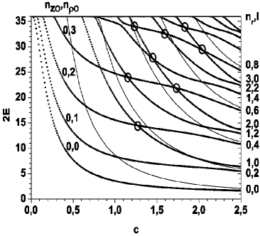
a) b)

Figure 2: The energies $2E=\tilde{E}/E_{R}$ of even $\sigma=+1$ lower states for OSQD versus the minor $c$, $\zeta_{ca}=c/a\in(1/5,1)$ being the spheroid aspect ratio: a) well with impermeable walls, b) diffusion potential with $2U_{0}=36$, $s=0.1$, the major semiaxis $a=2.5$ and $m=0$. Tine lines are minimal values $2E_{i}^{min}\equiv 2E_{i}(x_{s}=0)$ of potential curves.

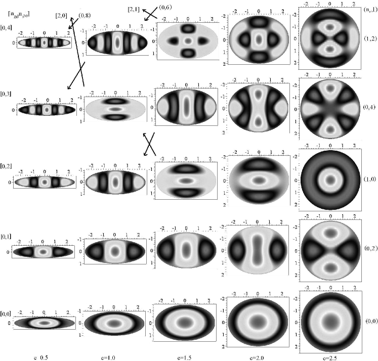
Figure 3: Contour lines of the first five even-parity wave functions $\sigma=+1$ in the $xz$ plane of Model B of OSQD for the major semiaxis $a=2.5$ and different values of the minor semiaxis $c$ ($\zeta_{ca}=c/a\in(1/5,1)$)

For Model B at $c=a=r_{0}$ the OSQD turns into SQD with known analytically expressed energy levels $E_{t}\equiv E_{nlm}^{sp}$ and the corresponding eigenfunctions

$$2E_{nlm}^{sp}\!=\!\frac{\alpha_{n_{r}+1,l+1/2}^{2}}{r_{0}^{2}},~{}\Phi_{nlm}^{sp}(r,\theta,\varphi)\!=\!\frac{\sqrt{2}J_{l+1/2}(\sqrt{2E_{nlm}^{sp}}r)}{r_{0}\sqrt{r}|J_{l+3/2}(\alpha_{n_{r}+1,l+1/2})|}Y_{lm}(\theta,\varphi),$$ (23)

where $\alpha_{n_{r}+1,l+1/2}$ are zeros of the Bessel function of semi-integer index $l+1/2$, numbered in ascending order $0<\alpha_{11}<\alpha_{12}<...<\alpha_{iv}<...$ by the integer $i,v=1,2,3,...$. Otherwise one can use equivalent pairs $iv\leftrightarrow\{n_{r},l\}$ with $n_{r}=0,1,2,...$ numbering the zeros of the Bessel function and $l=0,1,2,...$, being the orbital quantum number that determines the parity of states $\hat{\sigma}=(-1)^{l}=(-1)^{m}\sigma$, $\sigma=(-1)^{l-m}=\pm 1$. At fixed $l$, the energy levels $\tilde{E}_{nlm}/\tilde{E}_{R}=2E_{t}$ degenerate with respect to the magnetic quantum number $m$, are labelled with the quantum number $n=n_{r}+1=i=1,2,3,...$ , in contrast to the spectrum of a spherical oscillator, degenerate with respect to the quantum number $\lambda=2n_{r}+l$. Figs. 2, 3 show the lower part of the non-equidistant spectrum $\tilde{E}(\zeta_{ca})/\tilde{E}_{R}=2E_{t}$ and the eigenfunctions $\Psi^{m\sigma}_{t}$ from Eq. (13) for even states OSQD Models B and C at $m=0$. There is a one-to-one correspondence rule $n_{o}=n_{zo}+1=2n-(1+\sigma)/2,n=1,2,3,...$, between the sets of spherical quantum numbers $(n,l,m,\hat{\sigma})$ of SQD with radius $r_{0}=a=c$ and spheroidal ones $\{n_{\xi}=n_{r},n_{\eta}=l-|m|,m,\sigma\}$ of OSQD with the major $a$ and the minor $c$ semiaxes, and the adiabatic set of cylindrical quantum numbers $[n_{zo},n_{\rho o},m,\sigma]$ at continuous variation of the parameter $\zeta_{ca}=c/a$. The presence of crossing points of the energy levels of similar parity under the symmetry change from spherical $\zeta_{ca}=1$ to axial, i.e., under the variation of the parameter $0<\zeta_{ca}<1$, in the BVP with two variables at fixed $m$ for Model B is caused by the possibility of variable separation for Eq. (8) in the OSC [44], i.e., the r.h.s. of Eq. (17 ) equals zero, and by the existence of the integral of motion (9). The transformation of the eigenfunctions occurring in the course of a transition through the crossing points (marked by circles) in Fig. 2, is shown in Fig. 3 for model B (marked by arrows) and similar for model C. From the comparison of these Figures one can see that if the eigenfunctions are ordered in accordance with the increasing eigenvalues of the BVPs, then for both Models B and C, the number of nodes [47] is invariant under the variation of the parameter $c$ from $c=a=2.5$ to $c=0.5$ of the potentials (3) and (5). For Model B, such a behavior follows from the fact of separation of variables of the BVP with the potential (3) in the OSC, while for Model C further investigation is needed, because the coordinate system, in which the variables of the BVP with the potential (5) are separable, is unknown. So, at small values of the deformation parameter ($\zeta_{ca}$ for OSQD or $\zeta_{ac}$ for PSQD) there are nodes only along the corresponding major semiaxis. For Model C at each value of the parameter $a$ there is a finite number of discrete energy levels limited by the value $2U_{0}$ of the well walls height. As shown in Fig. 2b, the number of levels of OSQD, equal to that of SQD at $a=c=r_{0}$, is reduced with the decrease of the parameter $c$ (or $\zeta_{ca}$), in contrast to Models A and B that have countable spectra, and avoided crossings appear just below the threshold.

3.3 Models B and C for Prolate Spheroidal QD.

In contrast to OSQD, for PSQD at fixed coordinate $x_{s}$ of the slow subsystem the motion of the particle in the fast degree of freedom $x_{f}$ is confined to a 2D potential well with the effective variable radius

$$\rho_{0}\left(x_{s};a,c\right)=a\sqrt{1-{x_{s}^{2}}/{c^{2}}},$$ (24)

where $\rho_{0}\left(x_{s}\right)=\tilde{\rho}_{0}\left(x_{s}\right)/{a_{B}^{*}}$. The parametric BVP for Eq. (12) at fixed values of the coordinate $x_{s}$ from the interval $x_{s}\in(-c,c)$ is solved in the interval $x_{f}\in(0,\rho_{0}\left(x_{s}\right))$ for Model C using the program ODPEVP, while for Model B the eigenvalues $\tilde{E}_{n_{\rho p}+1}\left(x_{s}\right)/\tilde{E}_{R}\equiv 2E_{i}\left(x_{s}\right)$, $n_{\rho p}+1=i=1,2,...$, and the corresponding parametric basis functions $\Phi^{m\sigma=0}_{i}\left({x_{f};x_{s}}\right)\equiv\Phi^{m}_{i}\left({x_{f};x_{s}}\right)$ without parity separation are expressed in the analytical form:

$$2E_{i}\left(x_{s}\right)=\frac{\alpha_{n_{\rho p}+1,|m|}^{2}}{\rho_{0}^{2}\left(x_{s}\right)},\quad\Phi^{m}_{n_{\rho p}}(x_{s})=\frac{\sqrt{2}}{\rho_{0}\left(x_{s}\right)}\frac{J_{|m|}(\sqrt{2E_{n_{\rho p}+1,|m|}\left(x_{s}\right)}x_{f})}{|J_{|m|+1}(\alpha_{n_{\rho p}+1,|m|})|},$$ (25)

where $\alpha_{n_{\rho p}+1,|m|}=\bar{J}^{n_{\rho p}+1}_{|m|}$ are positive zeros of the Bessel function of the first kind $J_{|m|}(x_{f})$, labeled in the ascending order with the quantum number $n_{\rho p}+1=i=1,2,...$.

The effective potentials (18) in Eq.(17) for the slow subsystem are calculated numerically in quadratures via the integrals over the fast variable $x_{f}$ of the basis functions(25) and their derivatives with respect to the parameter $x_{s}$, and at $m=0$ may be presented in the analytical form:

$$2E_{i}\left(x_{s}\right)=\frac{(\bar{J}_{0}^{i})^{2}}{\rho_{0}^{2}\left(x_{s}\right)},\quad H_{ii}(x_{s})=\left(\frac{\rho_{0}^{\prime}\left(x_{s}\right)}{\rho_{0}\left(x_{s}\right)}\right)^{2}\frac{(1+\bar{J}_{0}^{i})}{3},$$ (26)

$$H_{ij}(x_{s})=2\left(\frac{\rho_{0}^{\prime}\left(x_{s}\right)}{\rho_{0}\left(x_{s}\right)}\right)^{2}\left(\bar{J}_{0}^{i}\bar{J}_{0}^{j}\int_{0}^{1}\frac{J_{1}(\bar{J}_{0}^{i}x)}{J_{1}(\bar{J}_{0}^{i})}\frac{J_{1}(\bar{J}_{0}^{j}x)}{J_{1}(\bar{J}_{0}^{j})}x^{3}dx\right.$$

$$\left.\qquad\qquad-\bar{J}_{0}^{i}\int_{0}^{1}\frac{J_{1}(\bar{J}_{0}^{i}x)}{J_{1}(\bar{J}_{0}^{i})}\frac{J_{0}(\bar{J}_{0}^{j}x)}{J_{1}(\bar{J}_{0}^{j})}x^{2}dx-\bar{J}_{0}^{j}\int_{0}^{1}\frac{J_{0}(\bar{J}_{0}^{i}x)}{J_{1}(\bar{J}_{0}^{i})}\frac{J_{1}(\bar{J}_{0}^{j}x)}{J_{1}(\bar{J}_{0}^{j})}x^{2}dx\right),$$

$$Q_{ij}(x_{s})=-2\frac{\rho_{0}^{\prime}\left(x_{s}\right)}{\rho_{0}\left(x_{s}\right)}\bar{J}_{0}^{j}\int_{0}^{1}\frac{J_{0}(\bar{J}_{0}^{i}x)}{J_{1}(\bar{J}_{0}^{i})}\frac{J_{1}(\bar{J}_{0}^{j}x)}{J_{1}(\bar{J}_{0}^{j})}x^{2}dx,\quad j\neq i.$$

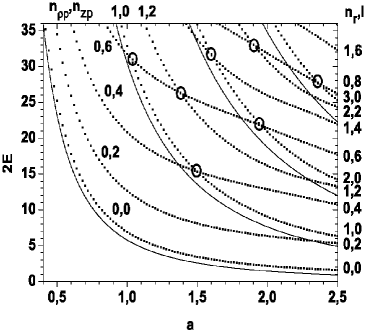
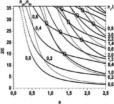
a) b)

Figure 4: The energies $2E=\tilde{E}/E_{R}$ of even $\sigma=+1$ lowest states for PSQD depending on the minor semiaxis $a$ $(\zeta_{ac}=a/c\in(1/5,1)$ is the spheroid aspect ratio): a) well with impermeable walls, b) diffusion potential, $2U_{0}=36$, $s=0.1$, for the major semiaxis $c=2.5$ and $m=0$. Tine lines are minimal values $2E_{i}^{min}\equiv 2E_{i}(x_{s}=0)$ of potential curves

Figures 4, 5 illustrate the lower part of the non-equidistant spectrum $\tilde{E}(\zeta_{ac})/\tilde{E}_{R}$ = $2E_{t}$ and the eigenfunctions $\Psi^{m\sigma}_{t}$ from Eq. (13) of even states of PSQD Models B and C.

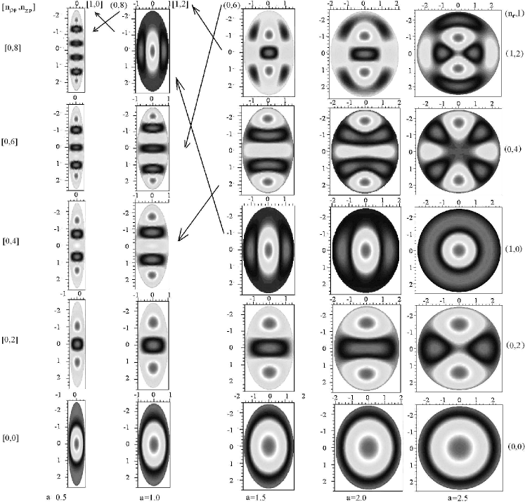
Figure 5: Contour lines of the first five even-parity wave functions $\sigma=+1$ in the $xz$ plane of Model B of PSQD for the major semiaxis $c=2.5$ and different values of the minor semiaxis $a$ ($\zeta_{ac}=a/c\in(1/5,1)$)

A one-to-one correspondence rule $n_{\rho p}+1=n_{p}=i=n=n_{r}+1$, $i=1,2,...$ and $n_{zp}=l-|m|$ holds between the quantum numbers $(n,l,m,\hat{\sigma})$ of SQD with the radius $r_{0}=a=c$, the spheroidal quantum numbers $\{n_{\xi}=n_{r},n_{\eta}=l-|m|,m,\sigma\}$ of PSQD with the major $c$ and the minor $a$ semiaxes, and the adiabatic set of quantum numbers $[n_{p}=n_{\rho p}+1,n_{zp},m,\sigma]$ under the continuous variation of the parameter $\zeta_{ac}=a/c$. The presence of crossing points of similar-parity energy levels in Fig. 4 under the change of symmetry from spherical $\zeta_{ac}=1$ to axial, i.e., under the variation of the parameter $0<\zeta_{ac}<1$, in the BVP with two variables at fixed $m$ for Model B is caused by the possibility of variable separation for Eq. (6) in the PSC  [44], i.e., r.h.s. of Eq. (17) equals zero, and by the existence of the additional integral of motion (7). For Model C, at each value of the parameter $c$ there is also only a finite number of discrete energy levels limited by the value $2U_{0}$ of the well walls height. As shown in Fig. 4b, the number of energy levels of PSQD, equal to that of SQD at $a=c=r_{0}$, which is determined by the product of mass $\mu_{e}$ of the particle, the well depth $\tilde{U}_{0}$, and the square of the radius $\tilde{r}_{0}$, is reduced with the decrease of the parameter $\tilde{a}$ (or $\zeta_{ac}$) because of the promotion of the potential curve (lower bound) into the continuous spectrum, in contrast to Models A and B having countable spectra. Note, that the spectrum of Model C for PSQD or OSQD should approach that of Model B with the growth of the walls height $U_{0}$ of the spheroidal well. However, at critical values of the ellipsoid aspect ratio it is shown that in the effective mass approximation, both the terms (lower bound) and the discrete energy eigenvalues in models of the B type are shifter towards the continuum. Therefore, when approaching the critical aspect ratio values, it is necessary to use such models, as the lens-shaped self-assembled QDs with a quantum well confined to a narrow wetting layer [4], or, if the minor semiaxis becomes comparable with the lattice constant, to proceed to models beyond the effective mass approximation (see,e.g.[48]).

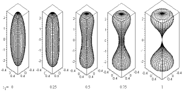
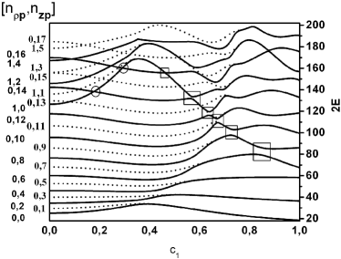
a b

Figure 6: a. The profile in plane $z,\rho$ of closed surface generated by rotating of continuous curve $\rho_{0}(z;a,c,c_{1})$ from (4) about z-axis for $c=2.5$, $a=0.5$ vs $c_{1}=0,0.25,0.5,0.75,1$. b. The energy levels of the even and odd states of DSQD for model B generated by (4) for $c=2.5$, $a=0.5$ vs $c_{1}$ classified at $c_{1}=0$ by adiabatic quantum numbers $n_{\rho p}$, $n_{zp}$ and $m=0$ of PSQD.

3.4 Models B for dumbbell QD

For DQD at the fixed coordinate $x_{s}$ of the slow subsystem the motion of the particle in the fast degree of freedom $x_{f}$ is confined to a 2D potential double well at $0\leq c_{1}\leq 1$ with the effective variable radius

$$\rho_{0}\left(x_{s}\right)\equiv\rho_{0}\left(x_{s};a,c,c_{1}\right)=\frac{a}{c}\sqrt{c^{2}-x_{s}^{2}}\frac{x_{s}^{2}c_{1}^{2}+1-c_{1}^{2}}{c_{1}^{2}c^{2}/4+1-c_{1}^{2}}.$$ (27)

Fig. 6 illustrates the transformation of the prolate spheroidal shape of QD with $c=2.5$ and $a=0.5$, considered in the previous Section, into a “dumbbell”-type shape and the corresponding evolution of the lower part of the countable spectrum $\tilde{E}(\zeta_{ac}=1/5,c_{1})/\tilde{E}_{R}$ = $2E_{t}$ of Model B versus the deformation parameter $c_{1}$ at a few fixed values $c_{1}=0,0.25,...,1$ from the interval $0\leq c_{1}\leq 1$. At $c_{1}=0$ the discrete spectrum states are characterized by a set of exact spheroidal or adiabatic cylindrical quantum numbers, $\{n_{\xi},n_{\eta},m,\sigma\}$ or [$n_{\rho p},n_{zp},m,\sigma$]. Typically, one can see exact crossing of energy levels having different parity ($\sigma=\pm 1$) with the growth of the deformation parameter $c_{1}$, which leads, first, to the quasidegeneracy of these energy levels and then to their exact degeneracy at the critical value $c_{1}=1$. On the other hand, for small values of the deformation parameter $c_{1}$ one observes, first, exact crossings (labelled with circles like in Fig.4a above) of similar-parity energy levels, replaced with the avoided crossings (labelled with squares) for greater values of the deformation parameter approaching the critical value $c_{1}=1$. A similar picture was observed in the example of a 2D-Sinai billiard [49], a 2D-quantum billiard with the shape $x^{2}+y^{2}+\epsilon x^{3}=1$ and the deformation parameter $\epsilon>0$, provided the so-called whispering gallery modes and considered in  [50, 51], as well as in the unidirectional far-field emission of coupled nonidentical microdisks  [16].

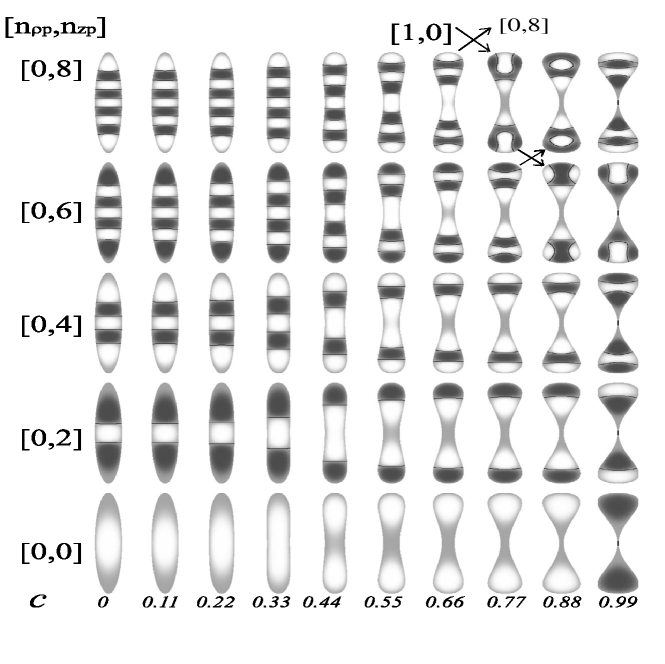
Figure 7: Contour lines of the first five eigenfunctions of model B of DSQD at $a=2.5$, $c=0.5$ and several values of $c_{1}$. Light and dark inflections are positive and negative values of eigenfunctions and lines are eigenfunction nodes. The adiabatic cylindrical quantum numbers [$n_{\rho p}$, $n_{zp}$] are given at $m=0$. Crossing arrows mean the transformation of nodes of pair of eigenfunctions after passing value of parameter in which avoided crossing of corresponding pair of eigenvalues was taking place in Fig. 6.b.

In Fig. 7 we show the evolution of the first five eigenfunctions with the increasing deformation parameter values $c_{1}=c_{1}=0,0.11,...,0.99$.

The transformation of eigenfunctions when passing the avoided crossing points (labelled with squares) in Fig. 6 b, is shown in Fig. 7 for model B of DQD (labelled with arrows). Comparing these Figures, one can see that if the eigenfunctions are ordered in accordance with the increasing eigenvalues of the BVPs, then the number of nodes is not invariant under the variation of the parameter $c_{1}$ from $c_{1}=0$ to $c_{1}=1$ in the potentials (27). In particular, in Fig. 7 one can see that the eigenfunction of the state $[n_{\rho p}=0,n_{zp}=6,m=0,\sigma=+1]$ at $c_{1}=0.99$ has the same number of nodes as the eigenfunction of the state $[n_{\rho p}=1,n_{zp}=0,m=0,\sigma=+1]$ at $c_{1}=0$. Above we could already observe this in Fig.5 at $a=1$ (up-going arrow) after several exact and avoided crossings of the corresponding energy levels in Fig. 6b). At the same time, the eigenfunction of the state $[n_{\rho p}=0,n_{zp}=8,m=0,\sigma=+1]$ at $c_{1}=0.99$ after avoided crossing of the corresponding energy levels in Fig. 6b) has the same number of nodes as the eigenfunction of the state $[n_{\rho p}=6,n_{zp}=0,m=0,\sigma=+1]$ at $c_{1}=0$.

4 Absorption Coefficient for an Ensemble of QDs

One can use the mentioned differences in the energy spectra to verify the considered models of QDs by calculating the absorption coefficient $K(\omega^{ph},\tilde{a},\tilde{c},)$ of an ensemble of identical semiconductor QDs [52]:

$$\tilde{K}(\tilde{\omega}^{ph},\tilde{a},\tilde{c})=\sum_{\nu,\nu^{\prime}}\tilde{K}_{\nu,\nu^{\prime}}(\tilde{\omega}^{ph},\tilde{a},\tilde{c})=\tilde{A}\sum_{\nu,\nu^{\prime}}\tilde{I}_{\nu,\nu^{\prime}}\delta(\hbar\tilde{\omega}^{ph}-\tilde{W}_{\nu\nu^{\prime}}),$$ (28)

$$\tilde{I}_{\nu,\nu^{\prime}}=|\int\tilde{\Psi}^{e}_{\nu}(\tilde{\vec{r}};\tilde{a},\tilde{c},)\tilde{\Psi}^{h}_{\nu^{\prime}}((\tilde{\vec{r}};\tilde{a},\tilde{c},))d\tilde{\vec{r}}|^{2},\,\,\,\,\tilde{W}_{\nu\nu^{\prime}}=\tilde{E}_{g}+\tilde{E}^{e}_{\nu}(\tilde{a},\tilde{c})+\tilde{E}^{h}_{\nu^{\prime}}(\tilde{a},\tilde{c}),$$

where $\tilde{A}$ is proportional to the square of the matrix element in the Bloch decomposition, $\tilde{\Psi}^{e}_{\nu}(u)$ and $\tilde{\Psi}^{h}_{\nu^{\prime}}$ are the eigenfunctions of an electron ($e$) and a heavy hole ($h$), $\tilde{E}^{e}_{\nu}$ and $\tilde{E}^{h}_{\nu^{\prime}}$ are the energy eigenvalues for an electron ($e$) and a heavy hole ($h$), depending on the semiaxis size $\tilde{c},\tilde{a}$ for OSQD (or $\tilde{a},\tilde{c}$ for PSQD) and the adiabatic set of quantum numbers $\nu=[n_{zo},n_{\rho o},m]$ and $\nu^{\prime}=[n_{zo}^{\prime},n_{\rho o^{\prime}},m^{\prime}]$ ($\nu=[n_{\rho p},n_{zp},m]$ and $\nu^{\prime}=[n_{\rho p}^{\prime},n_{zp}^{\prime},m^{\prime}]$), where $m^{\prime}=-m$, $\tilde{E}_{g}$ is the band gap width in the bulk semiconductor, $\tilde{\omega}^{ph}$ is the incident light frequency, $\tilde{W}_{\nu\nu^{\prime}}$ is the inter-band transition energy for which $\tilde{K}(\tilde{\omega}^{ph})$ has the maximal value. We rewrite the expression (28) using dimensionless quantities in reduced atomic units

$$\tilde{K}(\omega^{ph},\tilde{a},\tilde{c})=\tilde{A}\tilde{E}_{g}^{-1}\sum_{\nu,\nu^{\prime}}\tilde{I}_{\nu,\nu^{\prime}}\delta[f_{\nu,\nu^{\prime}}(u)],$$

$$f_{\nu,\nu^{\prime}}(u)=\lambda_{1}-(2E_{g})^{-1}(2E^{e}_{\nu}(a,c)+2E^{h}_{\nu^{\prime}}(a,c)(\mu_{h}/\mu_{e})),$$

where the parameter will $u$ be defined below, $\lambda_{1}=(\hbar\tilde{\omega}^{ph}-\tilde{E}_{g})/\tilde{E}_{g}$ is the energy of the optical interband transitions scaled to $\tilde{E}_{g}$, $2E_{g}=\tilde{E}_{g}/\tilde{E}^{e}_{R}=1.43/(5.27\cdot 10^{-3})$ is the dimensionless band gap width. For both electron and hole carriers the dimensionless energies $2E_{\nu}^{e}=\tilde{E}_{\nu}^{e}/\tilde{E}^{e}_{R}$ and $2E_{\nu}^{h}(\mu_{h}/\mu_{e})=\tilde{E}_{\nu}^{h}/\tilde{E}^{e}_{R}$ are expressed in the same reduced atomic units $\tilde{E}^{e}_{R}$.

Now consider an ensemble of OSQDs (or PSQDs) with different values of the minor semiaxis $c=u_{o}\bar{c}$ (or $a=u_{p}\bar{a}$) determined by the random parameter $u=u_{o}$ (or $u=u_{p}$). The corresponding minor semiaxis mean value is $\bar{c}$ at fixed major semiaxis $a$ (or $\bar{a}$ at fixed major semiaxis $c$) and the appropriate distribution function is $P(u_{o})$ (or $P(u_{p})$). Conventionally, they use the normalized Lifshits-Slezov $P(u)\equiv P^{LS}(u)$ [53] or Gaussian $P(u)\equiv P^{G}(u)$ distribution functions ($\int P(u)du=\int uP(u)du=1$):

$$P^{LS}(u):=\left\{\begin{array}[]{ll}\frac{3^{4}eu^{2}\exp(-1/(1-2u/3))}{2^{5/3}(u+3)^{7/3}(3/2-u)^{11/3}},&u\in(0,3/2);\\ 0,&\mbox{otherwise}\end{array}\right.$$

$$P^{G}(u):=1/\sqrt{2\pi}/\sigma\exp(-(u-1)^{2}/(2\sigma^{2})),$$

where $\bar{u}=\int uP^{G}(u)du=1$ is the mean value of $u$ and $\sigma^{2}=(\int(u-\bar{u})^{2}P^{G}(u)du)$ is the variance. The absorption coefficient of an ensemble of semiconductor QDs with different dimensions of minor semiaxes is then expressed as

$$\tilde{K}^{o}(\omega^{ph},\bar{\tilde{a}},\tilde{c})=\int\tilde{K}(\omega^{ph},\bar{\tilde{a}},\tilde{c},u_{o})P(u_{o})du_{o},$$

$$\tilde{K}^{p}(\omega^{ph},\tilde{a},\bar{\tilde{c}})=\int\tilde{K}(\omega^{ph},\tilde{a},\bar{\tilde{c}},u_{p})P(u_{p})du_{p}.$$

Taking the known properties of the $\delta$-function into account, we arrive at the analytical expression for the the absorption coefficient $\tilde{K}(\omega^{ph},\tilde{a},\tilde{c})$ of a system of semiconductor QDs with a distribution of minor semiaxes:

$$\frac{\tilde{K}(\omega^{ph})}{\tilde{K}_{0}}=\sum_{\nu,\nu^{\prime},s}\frac{\tilde{K}_{\nu,\nu^{\prime}}(\omega^{ph})}{\tilde{K}_{0}},\quad\frac{\tilde{K}_{\nu,\nu^{\prime}}(\omega^{ph})}{\tilde{K}_{0}}=\tilde{I}_{\nu,\nu^{\prime}}\left|\left.\frac{df_{\nu,\nu^{\prime}}(u)}{du}\right|_{u=u_{s}}\right|^{-1}P\left(u_{s}\right),$$ (29)

where $\tilde{K}_{0}=\tilde{A}^{-1}\tilde{E}_{g}$ is the normalization factor, $u_{s}$ are the roots of the equation $f_{\nu,\nu^{\prime}}(u_{s})=0$.

In particular, for Model B of OSQD or PSQD we have the interband overlap $\tilde{I}_{\nu,\nu^{\prime}}=\delta_{n_{\rho o},n_{\rho o}^{\prime}}\delta_{n_{zo},n_{zo}^{\prime}}\delta_{m,-m^{\prime}}$ for OSQD,
$\tilde{I}_{\nu,\nu^{\prime}}=(J_{1+|m|}(\alpha_{n_{\rho p}+1,|m|})/J_{1-|m|}(\alpha_{n_{\rho p}+1,|m|}))^{2}\delta_{n_{zp},n_{zp}^{\prime}}\delta_{n_{\rho p},n_{\rho p}^{\prime}}\delta_{m,-m^{\prime}}$ for PSQD, and the selection rules $n_{zo}=n_{zo}^{\prime}$, $n_{\rho o}=n_{\rho o}^{\prime}$, and $m=-m^{\prime}$ or $n_{\rho p}=n_{\rho p}^{\prime}$, $n_{zp}=n_{zp}^{\prime}$ and $m=-m^{\prime}$, respectively. Note that the contributions of non-diagonal matrix elements to the energy values are about 1% for OSQD and PSQD of Model B; then in the Born-Oppenheimer approximation of the order $b_{max}$ for the absorption coefficient we get

$$f_{\nu,\nu^{\prime}}(u)=\lambda_{1}-\sum_{j=0}^{b_{max}}\check{E}^{(j)}u^{j-2}.$$ (30)

Here the coefficients $\check{E}^{(j)}$ are defined by

$$\check{E}^{(j)}=(2E_{g})^{-1}E^{(j)}_{io}\omega_{\rho;n_{o}}^{2-j}(\bar{c})(1+\mu_{e}/\mu_{h})$$

$$\mbox{or}\quad\check{E}^{(j)}=(2E_{g})^{-1}E^{(j)}_{ip}\omega_{z;n_{\rho p}}^{2-j}(\bar{a})(1+\mu_{e}/\mu_{h}).$$ (31)

$$\omega_{\rho;n_{o}}(\bar{c})=\pi n_{o}/(a\bar{c}),\quad\omega_{z;n_{\rho p}}(\bar{a})=\alpha_{n_{\rho p}+1,|m|}/(\bar{a}c).$$ (32)

$$E^{(0)}_{io}=a^{2}/4,\quad E^{(1)}_{io}=(2n_{\rho o}\!+\!{|m|}\!+\!1),$$

$$E^{(2)}_{io}=(6n_{\rho o}{|m|}\!+\!2\!+\!6n_{\rho o}\!+\!6n_{\rho o}^{2}\!+\!{|m|}^{2}\!+\!3{|m|})a^{\!-\!2},$$ (33)

$$E^{(3)}_{io}=\!3(6n_{\rho o}\!+\!3{|m|}\!+\!2\!+\!{|m|}^{2}\!+\!6n_{\rho o}^{2}\!+\!6n_{\rho o}{|m|}\!+\!4n_{\rho o}^{3}$$

$$~{}~{}~{}~{}+\!6{|m|}n_{\rho o}^{2}\!+\!2{|m|}^{2}n_{\rho o})a^{\!-\!4}/2,$$ (34)

$$E^{(0)}_{ip}=c^{2},\quad E^{(1)}_{ip}=(2n_{zp}\!+\!1),\quad E^{(2)}_{ip}=\!+\!3(2n_{zp}\!+\!2n_{zp}^{2}\!+\!1)c^{-2}/4,$$

$$E^{(3)}_{ip}=\!3(3n_{zp}^{2}\!+\!7n_{zp}\!+\!2n_{zp}^{3}\!+\!3)c^{-4}/16.$$

The coefficients of the order $b_{\max}\geq 4$ are calculated by the perturbation theory algorithms [34, 35] using exact solutions of 2D and 1D oscillators with adiabatic frequencies $\omega_{\rho;n_{o}}(\bar{c})$ and $\omega_{z;n_{\rho p}}(\bar{a})$ from (32) that distinguish from conventional ones, for example, $\omega_{\rho}$ and $\omega_{z}$ using in section 3.1 or in [18, 24]. The accuracy of such approximations up to $b_{\max}=5$ is about 4 – 6 decimal digits in comparison with the numerical results of the crude diagonal adiabatic approximation (CDAA) of Eqs.(17) without $H_{ii}(x_{s})$ for the states from Fig. 2a at $c=0.5$ and Fig. 4a at $a=0.5$. In the case $a=c=1$ the accuracy is only about two decimal digits in comparison with the CDAA of the exact spectrum Eq. (23) of model B of SQDs [52].

Note that in model B $2E_{io}$ and $2E_{ip}$ monotonically depend upon the parameter $u$ and, therefore, the algebraic equation $f_{\nu,\nu^{\prime}}(u)=0$ has the only solution in the considered domain of definition. Using the notations $\lambda_{1}^{\prime}=\lambda_{1}$ for $b_{max}=1$ and $\lambda_{1}^{\prime}=\lambda_{1}-E^{(2)}_{io}$, or $\lambda_{1}^{\prime}=\lambda_{1}-E^{(2)}_{ip}$ for $b_{max}\geq 2$, we rewrite this equation in the Born-Oppenheimer approximations up to the third order $b_{max}\leq 3$

$$f_{\nu,\nu}(u)=\lambda^{\prime}_{1}-\check{E}^{(0)}u^{-2}-\check{E}^{(1)}u^{-1}-\check{E}^{(3)}u=0,$$

which has the required roots $u_{1}=u_{1}^{(b_{max})}$:

$$u_{1}^{(1,2)}=(2\lambda_{1}^{\prime})^{-1}(\check{E}^{(1)}+((\check{E}^{(1)})^{2}+4\lambda_{1}^{\prime}\check{E}^{(0)})^{1/2})),$$

$$u_{1}^{(3)}=u^{(2)}+\check{E}^{(3)}(u_{1}^{(2)})^{4}/(2\check{E}^{(0)}+\check{E}^{(1)}u_{1}^{(2)}).$$

Figure 8: Absorption coefficient $K/K_{0}$ from (29) consists of sum of the first partial contributions vs the energy $\lambda=\lambda_{1}$ of the optic interband transitions for the Lifshits-Slezov distribution in first, second and third (from left to right) Born Oppenheimer approximations: (top panels) for assemble of OSQDs $\bar{c}=0.5$, $a=2.5$ (summation by $n_{o}=1,2,3$, $n_{\rho o}=0,1,2,3,4,5$, $m=0$), (bottom panels) for assemble of PSQDs $\bar{a}=0.5$, $c=2.5$ (summation by $n_{p}=1,2,3$, $n_{zp}=0,1,2,3,4,5$, $m=0$).

For the Lifshits-Slezov distribution Fig. 8 displays the total absorption coefficients ${\tilde{K}(\omega^{ph})}/{\tilde{K}_{0}}$ and the partial absorption coefficients ${\tilde{K}_{\nu,\nu}(\omega^{ph})}/{\tilde{K}_{0}}$, that form the corresponding partial sum (29) over a fixed set of quantum numbers $\nu$ at $m=-m^{\prime}=0$. One can see that the summation over the quantum numbers $n_{zo}$ (or $n_{\rho p}$) numerating the nodes of the wave function with respect to the fast variable gives the corresponding main maxima of the total absorption coefficients for the ensemble of QDs with distributed dimensions of minor semiaxis, while the summation over the quantum number $n_{\rho o}$ (or $n_{zp}$) that label the nodes of the wave function with respect to the slow variable leads to the increase of amplitudes of these maxima and to appearing secondary maxima in the case of sparer energy levels of Model B OSQDs (or PSQDs)

In the regime of strong dimensional quantization the frequencies of the interband transitions between the levels $n_{o}=1,n_{\rho o}=0,m=0$ for OSQD or $n_{p}=1,n_{zp}=0,m=0$ for PSQD in the BO1, at the fixed values $\tilde{a}=2.5a_{e}$ and $\tilde{c}=0.5a_{e}$ for OSQD or $\tilde{a}=0.5a_{e}$ and $\tilde{c}=2.5a_{e}$ for PSQD, are equal to $\tilde{\omega}^{ph}_{100}=2.17\times 10^{13}$ s^-1 or $\tilde{\omega}^{ph}_{100}=3.32\times 10^{13}$ s^-1 ($\tilde{\omega}^{ph}_{100}=\hbar^{-1}\tilde{W}_{100,100}$ with the accuracy to $3\%$ and $0.5\%$, respectively), corresponding to the infrared spectral region [6, 7]. With decreasing semiaxis the threshold energy increases, because the “effective” band gap width increases, which is a consequence of the enhancement of dimensional quantization. Therefore, the above frequency is greater for PSQD than for OSQD, because the SQ implemented in two direction of the plane (x,y) is effectively greater than that in the direction of the $z$ axis solely at similar values of semiaxes. Higher-accuracy calculations reveal an essential difference in the frequency behavior of the absorption coefficient for interband transitions (see Fig. 9) in systems of semiconductor OSQDs or PSQDs having a distribution of minor semiaxes, which can be used to verify the above models.

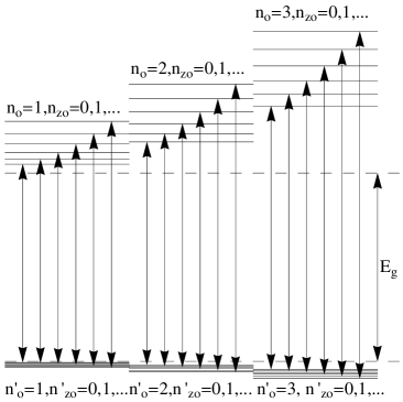
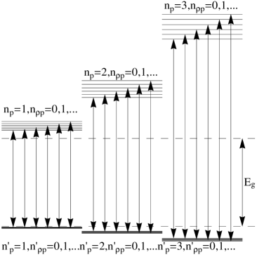
Figure 9: Schematic plots of interband transition corresponded to Fig. 8.

5 Conclusions

The presented examples of the analysis of energy spectra of SQD, OSQD, PSQD, and DQD models with three types of axially symmetric potentials demonstrate the efficiency of the developed computational scheme and SNA. Only Model A (anisotropic harmonic oscillator potential) is shown to have an equidistant spectrum, while Models B and C (wells with infinite and finite walls height) possess non-equidistant spectra. In Model C, there is a finite number of energy levels. This number becomes smaller as the parameter $a$ or $c$ ($\zeta_{ac}$ or $\zeta_{ca}$) is reduced because the potential curve (lower bound) moves into the continuum. Models A and B have countable discrete spectra. This difference in spectra allows verification of SQD, OSQD, and PSQD models using the experimental data [2], e.g., photoabsorption, from which not only the energy level spacing, but also the mean geometric dimensions of QD may be derived [6, 10, 11]. The considered examples of calculating the absorption coefficient for ensembles of OSQDs or PSQD’s with random minor semi-axes in model B have proved the possibility of a similar verification. It is shown that there are critical values of the ellipsoid aspect ratio, at which in the approximation of effective mass the discrete spectrum of the models with finite-wall potentials turns into a continuous one. Hence, using the experimental data, it is possible to verify different QD models like the lens-shaped self-assembled QDs with a quantum well confined to a narrow wetting layer [4], or to determine the validity domain of the effective mass approximation, if a minor semiaxis becomes comparable with the lattice constant and to proceed opportunely to more adequate models such as [48].

Further development of the method, symbolic-numerical algorithms, and the software package is planned for solving the quasi-2D and quasi-1D BVPs with both discrete and continuous spectrum, which are necessary for calculating the optical transition rates, channeling and transport characteristics in the models like quantum wells or quantum wires and low-energy barrier nuclear reactions.

The authors thank Profs. V.P. Gerdt and V.A. Rostovtsev for collaboration and Profs. V. I. Furman, L.G. Mardoyan, G.S. Pogosyan for useful discussions. This work was done within the framework of the Protocols No. 3967-3-6-09/11 and 4038-3-6-10/13 of collaboration between JINR (Dubna), RAU (Erevan) and SSU (Saratov) in dynamics of low dimensional quantum models and nanostructures in external fields. The work was supported partially by RFBR (grants 10-01-00200 and 11-01-00523), and by the grant No. MK-2344.2010.2 of the President of Russian Federation.

References

- [1] P. Harrison, Quantum Well, Wires and Dots (Wiley, New York, 2005).
- [2] K.M. Gambaryan, Nanoscale Res Lett., DOI 10.1007/s11671-009-9510-8 (2009)
- [3] V. A. Harutyunyan et al, Phys. E 36, 114 (2007).
- [4] A. Wojs et al, Phys. Rev. B 54, 5604 (1996).
- [5] L.A. Juharyan et al, Solid State Comm. 139, 537 (2006).
- [6] K.G. Dvoyan et al,Nanoscale Res. Lett. 2, 601 (2007).
- [7] K.G. Dvoyan et al,Nanoscale Res. Lett. 4, 106 (2009); Proc. SPIE 7998, 79981F (2010).
- [8] Y. E. Kim and A. L. Zubarev, Phys. Lett. A 289, 155 (2001).
- [9] G. Cantele et al, J. Phys. Condens. Matt. 12, 9019 (2000).
- [10] F. Trani et al, Phys. Rev. B 72, 075423 (2005).
- [11] A.-M. Lepadatu et al, J. Appl. Phys. 107, 033721 (2010).
- [12] A. Bagga, P. K. Chattopadhyay, and S. Ghosh, arXiv: cond-mat/0406517v1 (2004).
- [13] I. Filikhin et al. Physica E 41 (2009) 1358–1363
- [14] J. Gravesen and M. Willatzen Phys. Rev A 72, 032108 (2005)
- [15] G. N. Afanasiev Phys. Part. Nucl. 21, 172 (1990).
- [16] J.-W. Ryu et al Phys. Rev. A 79, 053858 (2009).
- [17] S. Granger and R.D. Spencer, Phys. Rev. 83, 460 (1951).
- [18] A.J. Rassey, Phys. Rev. 109, 949 (1958).
- [19] Y. Ayant and R. Arvieu, J. Phys. A 20, 397 (1987).
- [20] F. Brut and R. Arvieu, J. Phys. A 26, 4749 (1993).
- [21] V. V. Pashkevich and V. M. Strutinsky, Yad. Fiz. USSR 9, 56 (1969).
- [22] J. Damgaard et al, Nucl. Phys. A 135, 432 (1969).
- [23] J. Maruhn and W. Greiner, Z. Physik 251, 431 (1972).
- [24] D.N. Poenaru et al, Phys. Lett. A 372, 5448 (2008).
- [25] H. Hofmann, Nucl. Phys. A 224, 116 (1974).
- [26] B. Buck and A. A. Pilt, Nucl. Phys A 80, 133 (1977).
- [27] S. G. Kadmensky, V. I. Furman, Alpha decay and related nuclear Reactions (Moscow, 1985).
- [28] K. Hagino et al, Comput. Phys. Commun. 123, 143–152 (1999)
- [29] V. I. Zagrebaev and V. V. Samarin, Phys. At. Nucl. 67, 1462 (2004).
- [30] V. I. Zagrebaev et.al., Phys. Part. Nucl. 38, 469 (2007).
- [31] L.V. Kantorovich and V.I. Krylov, Approximate Methods of Higher Analysis (Wiley, NY, 1964).
- [32] A.A. Gusev et al, Math. Comp. in Simulation (2011) (accepted); arXiv:1005.2089
- [33] M. Born and X. Huang, Dynamical Theory of Crystal Lattices (The Clarendon, Oxford, 1954).
- [34] O. Chuluunbaatar et al, Lect. Notes Comp. Sci 4770, 118 (2007).
- [35] S.I. Vinitsky et al, Lect. Notes Comp. Sci 5743, 334 (2009).
- [36] A.A. Gusev et al, Lect. Notes Comp. Sci. 6244, 106 (2010).
- [37] O. Chuluunbaatar et al, Comput. Phys. Commun. 180, 1358 (2009).
- [38] O. Chuluunbaatar et al, Comput. Phys. Commun. 177, 649 (2007).
- [39] Yu.N. Demkov JETP 36, 88-92 (1959).
- [40] Yu.N. Demkov JETP 44, 2007-2010 (1963).
- [41] L.A. Il’kaeva Vestnik LGU, 22, 56-63 (1963).
- [42] H.E. Erikson and E.L. Hill, Phys.Rev. 75, 29 (1949).
- [43] L.G. Mardoyan et al, Preprint JINR, P2-85-139, Dubna, 1985.
- [44] M. Abramowitz and I.A. Stegun, Handbook of Mathematical Functions (Dover, New York, 1965).
- [45] L.G. Mardoyan et al Quantum systems with hidden symmetry (Fizmatlit, Moscow, 2006).
- [46] E. G. Kalnins et al J. Math. Phys. 43, 3592 (2002).
- [47] R. Courant and D. Hilbert, Methods of Mathematical Physics. V. 1 (Wiley, New York, 1989).
- [48] P.G. Harper, Proc. Phys. Soc. A 68, 874 (1955).
- [49] P.G. Akishin, F. Bosco, and S.I. Vinitsky, Comput. Math. Appl. 34, 613 (1997).
- [50] J. E. Bayfield, Quantum Evolution An Introduction to Time-Dependent Quantum Mechanics (John Wiley & Sons, Inc., New York, 1999), p. 207.
- [51] B. Crespi, G. Perez, and S.-J. Chang, Phys.Rev. E 47, 986 (1993).
- [52] Al.L. Efros, A.L. Efros, Sov. Phys. Semicond. 16, 772 (1982).
- [53] I.M. Lifshits and V.V. Slezov, Sov. Phys. JETF. 35, 479 (1958).