“Ultimate state” of two-dimensional Rayleigh-Bénard convection
between free-slip fixed-temperature boundaries

Abstract

Rigorous upper limits on the vertical heat transport in two dimensional Rayleigh-Bénard convection between stress-free isothermal boundaries are derived from the Boussinesq approximation of the Navier-Stokes equations. The Nusselt number Nu is bounded in terms of the Rayleigh number Ra according to $\mbox{Nu}\leq 0.2295\,Ra^{5/12}$ uniformly in the Prandtl number $\Pr$. This Nusselt number scaling challenges some theoretical arguments regarding the asymptotic high Rayleigh number heat transport by turbulent convection.

Rayleigh-Bénard convection is the buoyancy-driven flow of a fluid heated from below and cooled from above. It is important for a variety of systems in the engineering, geophysical, and astrophysical sciences, and it has long served as a fundamental paradigm of nonlinear science, chaos, and pattern formation. Indeed, the Boussinesq approximation to the Navier-Stokes equations with the boundary conditions analyzed in this paper was Rayleigh’s original model for calculating conditions for onset Rayleigh (1916), it is the basis of the Lorenz equations Lorenz (1963), and it formed the foundation of developments in the modern mathematical theory of amplitude Malkus and Veronis (1958) and modulation Newell and Whitehead (1969) equations. Most recently Rayleigh-Bénard convection has been the focus of a large body of experimental, computational, theoretical, and mathematical research aimed at characterizing the fully turbulent dynamics for application in geophysical and astrophysical regimes Ahlers et al. (2009).

Convective fluid flow increases vertical heat transport beyond the purely conductive flux. The dimensionless enhancement factor, the Nusselt number Nu, is both of fundamental interest for applications and the natural and widely recognized measure of the intensity and effectiveness of the motion. The most basic question for Rayleigh-Bénard convection is the dependence of Nu on (i) the strength of the thermal forcing, commonly expressed in terms of a dimensionless Rayleigh number Ra, (ii) the material properties of the fluid, which within the Boussinesq approximation is set by the dimensionless Prandtl number $\Pr$, the ratio of the fluid’s momentum and thermal diffusion coefficients, (iii) the geometry, typically the aspect ratio of the container, and (iv) the boundary conditions. The connection between these variables is generally complex and often not even unique, but in the “ultimate” high Rayleigh number regime when the flow is turbulent, the presumed functional relation between the Nu, $\Pr$, and Ra is $\mbox{Nu}\sim\Pr^{\gamma}\mbox{Ra}^{\beta}$.

Experiments and simulations with $\Pr={\cal O}(1)$ and no-slip boundary conditions suggest a scaling exponent $0.27\lesssim\beta\lesssim 0.40$ at the highest available Ra Ahlers et al. (2009); Roche et al. (2010). Various theories suggest (modulo possible logarithmic corrections) that $\mbox{Nu}\sim\Pr^{1/2}\mbox{Ra}^{1/2}$ as $\mbox{Ra}\rightarrow\infty$ Kraichnan (1962); Spiegel (1971); Grossman and Lohse (2000). Rigorous analyses of the Boussinesq model with no-slip velocity and isothermal (fixed temperature) Howard (1963); Doering and Constantin (1996) or fixed heat flux Otero et al. (2002) or mixed temperature Wittenberg (2010) boundary conditions yield upper bounds of the form $\mbox{Nu}\leq c\,\mbox{Ra}^{1/2}$ with prefactors $0<c<\infty$ independent of $\Pr$, so $\beta=\frac{1}{2}$ and $\gamma=\frac{1}{2}$ cannot both hold for very large $\Pr$. The Nu-Ra relation is certainly different at $\Pr=\infty$ where theory suggests Malkus (1954) and analysis proves Doering et al. (2006) (modulo possible logarithmic corrections) that $\mbox{Nu}\lesssim\mbox{Ra}^{1/3}$.

Two dimensional Rayleigh-Bénard convection displays many of the physical and turbulent transport features of three dimensional convection and has long been utilized as a test-bed for theoretical concepts DeLuca et al. (1990); Johnston and Doering (2009). The effect of free-slip (no-stress) velocity boundary conditions on developed turbulent convection has largely been unexplored although we note that the rigorous scaling bound reported here was anticipated by recent numerical and perturbative investigations of transport limits for finite Otero (2002) and infinite Ierley and Worthing (2001); Ierley et al. (2006) Prandtl numbers. This letter bridges that gap with a proof that $\mbox{Nu}\leq 0.2295\,Ra^{5/12}$ uniformly in $0<\Pr\leq\infty$ for the Boussinesq model in two spatial dimensions with fixed temperature and free-slip boundaries. This result refutes predictions of a $\mbox{Nu}\sim Ra^{1/2}$ ultimate regime insofar as the theoretical arguments do not refer specifically to the boundary conditions or the spatial dimension. This issue is discussed further in the conclusion section at the end of the paper. Meanwhile the proof of the bound is presented in sufficient detail immediately below for motivated readers to reproduce the calculation in its entirety. The key new idea used to derive the result emerged from intuition developed in numerical studies of upper bounds Ierley and Worthing (2001); Otero (2002): implement and exploit the bulk averaged enstrophy balance available for two-dimensional flows with free-slip boundaries to decrease the upper bound.

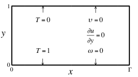
Figure 1: Geometry for the 2d stress-free convection problem. Boundary conditions for $T$, $u$, $v$, and the vorticity $\omega$ at the isothermal no-slip vertical boundaries are shown. All these variables as well as the pressure $p$ are periodic in the horizontal direction with period $\Gamma$.

The dimensionless equations of motion for the Boussinesq approximation are

$$\frac{1}{\Pr}\left(\frac{\partial\mbox{\boldmath$u$}}{\partial t}+\mbox{\boldmath$u$}\cdot\nabla\mbox{\boldmath$u$}\right)+\nabla p = \nabla^{2}\mbox{\boldmath$u$}+\mbox{Ra}\,\mbox{\boldmath$\hat{j}$}\,T,$$ (1)

$$\nabla\cdot\mbox{\boldmath$u$} = 0,$$ (2)

$$\frac{\partial T}{\partial t}+\mbox{\boldmath$u$}\cdot\nabla T = \nabla^{2}T,$$ (3)

where the Prandtl number $\Pr=\nu/\kappa$ is the ratio of the fluid’s kinematic viscosity $\nu$ to its thermal diffusivity $\kappa$, and the Rayleigh number $\mbox{Ra}=g\,\alpha\,\Delta T\,h^{3}/\nu\,\kappa$ where $g$ is the acceleration of gravity, $\alpha$ is the fluid’s thermal expansion coefficient, and $\Delta T$ is the imposed temperature drop across the layer of thickness $h$. Lengths are measured in units of $h$, time in units of $h^{2}/\kappa$, and temperature in units of $\Delta T$. The velocity vector field $\mbox{\boldmath$u$}(x,y,t)=\mbox{\boldmath$\hat{i}$}u(x,y,t)+\mbox{\boldmath$\hat{j}$}v(x,y,t)$ satisfies no-penetration and free-slip (stress-free) boundary conditions, and the temperature field $T(x,y,t)$ is isothermal on the vertical boundaries at $y=0$ and $y=1$ as shown in Fig. 1. All dependent variables, $u$, $v$, $T$, and the pressure field $p(x,y,t)$, are periodic in the horizontal direction $x$ with period $\Gamma$ (the aspect ratio).

Taking the curl of (1) one obtains the evolution equation for the scalar vorticity $\omega=\partial v/\partial x-\partial u/\partial y$,

$$\frac{1}{\Pr}\left(\frac{\partial\omega}{\partial t}+\mbox{\boldmath$u$}\cdot\nabla\omega\right)=\nabla^{2}\omega+\mbox{Ra}\,\frac{\partial T}{\partial x}.$$ (4)

The boundary conditions on $u$ and $v$ imply that $\omega=0$ on the vertical boundaries at $y=0$ and $y=1$.

The goal of the analysis is to use the equations of motion to derive upper bounds on the Nusselt number defined as $\mbox{Nu}=1+\langle vT\rangle$, where $\langle\cdot\rangle$ represents the spatial and long time average, in terms of Ra, $\Pr$, and $\Gamma$. Toward this end we utilize the background method Doering and Constantin (1992), a mathematical device introduced by Hopf to establish the existence of weak solutions to the Navier-Stokes equations in bounded domains Hopf (1941). For convection problems the background method involves decomposing the temperature field into a background profile $\tau(y)$ which satisfies the vertical boundary conditions ($\tau(0)=1$ and $\tau(1)=0$) and a perturbation term $\theta(x,y,t)$ satisfying corresponding homogeneous boundary conditions ($\theta(x,0,t)=0=\theta(x,1,t)$) so that $T(x,y,t)=\tau(y)+\theta(x,y,t)$ Doering and Constantin (1996). Implementing this decomposition the temperature equation (3) implies

$$\frac{\partial\theta}{\partial t}+\mbox{\boldmath$u$}\cdot\nabla\theta=\nabla^{2}\theta+\tau^{\prime\prime}(y)-v\tau^{\prime}(y).$$ (5)

Then the equations of motion together with the boundary conditions and the background decomposition imply

$$\frac{1}{2\Pr}\frac{d}{dt}\|\mbox{\boldmath$u$}\|_{2}^{2} = -\|\omega\|_{2}^{2}+\mbox{Ra}\int v\,\theta\,dxdy$$ (6)

$$\frac{1}{2\Pr}\frac{d}{dt}\|\omega\|_{2}^{2} = -\|\nabla\omega\|_{2}^{2}+\mbox{Ra}\int\omega\,\frac{\partial\theta}{\partial x}\,dxdy$$ (7)

$$\frac{1}{2}\frac{d}{dt}\|\theta\|_{2}^{2} = -\|\nabla\theta\|_{2}^{2}-\int\left[\tau^{\prime}\frac{\partial\theta}{\partial y}+\tau^{\prime}v\theta\right]dxdy$$ (8)

$$\|\nabla T\|_{2}^{2} = \|\nabla\theta\|_{2}^{2}+2\int\tau^{\prime}\frac{\partial\theta}{\partial y}dxdy+\|\tau^{\prime}\|_{2}^{2}$$ (9)

where $\|\cdot\|_{2}$ is the $L^{2}$ norm on the spatial domain and the elementary identity $\|\nabla\mbox{\boldmath$u$}\|_{2}^{2}=\|\omega\|_{2}^{2}$ was used in (6).

It is well-known that the equations of motion imply $\mbox{Nu}=\langle|\nabla T|^{2}\rangle$ Howard (1963); Doering and Constantin (1996). Thus, given coefficients $a$ and $b$ with precise values to be determined, combining (6-9) according to

$$\frac{b}{\mbox{Ra}}\times\eqref{eq:energy_mom}+\frac{a}{\mbox{Ra}^{3/2}}\times\eqref{eq:energy_omega}+2\times\eqref{eq:energy_theta}+\eqref{eq:energy_T},$$ (10)

applying the long time average—remarking that it can be shown within the background method that the time averages of the time derivatives vanish Doering and Constantin (1992, 1996)—and dividing by $\Gamma$, the Nusselt number is expressed

$$\mbox{Nu}=\frac{1}{1-b}\left(\int_{0}^{1}\tau^{\prime}(y)^{2}dy-b\right)-\frac{1}{1-b}\,\mathcal{Q}$$ (11)

where

$$\mathcal{Q} = \left\langle|\nabla\theta|^{2}\ +\ \frac{a}{\mbox{Ra}^{3/2}}|\nabla\omega|^{2}\ +\ \frac{b}{\mbox{Ra}}|\omega|^{2}\right.$$ (12)

$$+ 2\left.\tau^{\prime}\,v\,\theta\ +\ \frac{a}{\mbox{Ra}^{1/2}}\omega\,\frac{\partial\theta}{\partial x}\right\rangle.$$

Hence if we can choose the background profile $\tau(y)$ and coefficients $a>0$ and $0<b<1$ so that $\mathcal{Q}\geq 0$ for all relevant $\theta$, $\omega$ and $v$, then the first term on the right hand side of (11) is an upper bound on Nu. For the problem at hand we may use the piece-wise linear profile shown in Fig. 2 where the thickness $\delta$ of the “boundary layers” is to be determined as a function of Ra to satisfy $\mathcal{Q}\geq 0$. With this choice of $\tau(y)$ the bound will be

$$\mbox{Nu}\leq\frac{1}{2\delta(1-b)}-\frac{b}{1-b}.$$ (13)

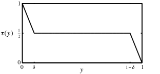
Figure 2: Background profile with boundary layers of thickness $0<\delta\leq\frac{1}{2}$ in which $\tau^{\prime}(y)=-\frac{1}{2\delta}$; $\tau^{\prime}(y)\equiv 0$ for $\delta<y<1-\delta$.

Applying the horizontal Fourier transform and introducing the shorthand $D=\frac{d}{dy}$, it is evident that positivity of $\mathcal{Q}$ is equivalent to the positivity of

$$\mathcal{Q}_{k}\ =\ \|D\hat{\theta}_{k}\|^{2}+k^{2}\|\hat{\theta}_{k}\|^{2} + \frac{a}{\mbox{Ra}^{3/2}}\|D\hat{\omega}_{k}\|^{2}$$

$$+\frac{a}{\mbox{Ra}^{3/2}}k^{2}\|\hat{\omega}_{k}\|^{2} + \frac{b}{\mbox{Ra}}\|\hat{\omega}_{k}\|^{2}$$ (14)

$$+\ \text{Re}\left\{2\int_{0}^{1}\tau^{\prime}\,\hat{v}_{k}\,\hat{\theta}^{*}_{k}dy\right. - \left.\frac{aik}{\mbox{Ra}^{1/2}}\int_{0}^{1}\hat{\omega}_{k}\,\hat{\theta}^{*}_{k}dy\right\}$$

for each horizontal wavenumber $k$ where $\|\cdot\|$ is now the $L^{2}$ norm on complex valued functions of $y\in[0,1]$ and $\text{Re}\left\{\cdot\right\}$ indicates the real part of a complex quantity. The Cauchy-Schwarz and Young inequalities imply

$$\left|\frac{a\,i\,k}{\mbox{Ra}^{1/2}}\int_{0}^{1}\hat{\omega}_{k}\hat{\theta}^{*}_{k}dy\right|\ \leq\ \frac{a^{2}}{4\mbox{Ra}}\|\ \hat{\omega}_{k}\|^{2}+k^{2}\|\hat{\theta}_{k}\|^{2}$$ (15)

so dropping the manifestly non-negative term $\|D\hat{\omega}_{k}\|^{2}$,

$$\mathcal{Q}_{k}\ \geq\ \|D\hat{\theta}_{k}\|^{2}+\left[\frac{ak^{2}}{\mbox{Ra}^{3/2}}\right. + \left.\frac{1}{\mbox{Ra}}\left(b-\frac{a^{2}}{4}\right)\right]\|\ \hat{\omega}_{k}\|^{2}$$

$$-\frac{1}{\delta}\,\text{Re}\left\{\int_{0}^{\delta}\hat{v}_{k}(y)\hat{\theta}_{k}^{*}(y)dy\right. + \left.\int_{1-\delta}^{1}\hat{v}_{k}(y)\hat{\theta}_{k}^{*}(y)dy\right\}.$$ (16)

Restricting $a^{2}<4b$, the task is to dominate the indefinite boundary layer integrals by the positive definite terms.

The Fourier coefficients of the vertical velocity and vorticity (suppressing the time dependence) are related by

$$ik\ \hat{\omega}_{k}(y)=D^{2}\hat{v}_{k}(y)-k^{2}\hat{v}_{k}(y).$$ (17)

Integrating the modulus squared of both sides with a simple integration by parts implies

$$k^{2}\|\ \hat{\omega}_{k}\|_{2}^{2}=\|D^{2}v_{k}\|^{2}+2k^{2}\|Dv_{k}\|^{2}+k^{4}\|v_{k}\|^{2}.$$ (18)

On the other hand, integration by parts and the Cauchy-Schwarz and Young inequalities yield

$$\frac{2}{3}k^{2}\|D\hat{v}_{k}\|^{2}\ \leq\ \frac{1}{9}\|D^{2}\hat{v}_{k}\|_{2}^{2}+k^{4}\|\hat{v}_{k}\|^{2}$$ (19)

so that, combining (18) and (19),

$$k^{2}\|\hat{\omega}_{k}\|_{2}^{2}\geq\frac{8}{9}\|D^{2}\hat{v}_{k}\|^{2}+\frac{8}{3}k^{2}\|D\hat{v}_{k}\|^{2}.$$ (20)

Boundary conditions on $\hat{v}_{k}(y)$ dictate that

$$\int_{0}^{1}\text{Re}\left\{D\hat{v}_{k}(y)\right\}dy=\left.\text{Re}\left\{\hat{v}_{k}(y)\right\}\right|_{z=0}^{z=1}=0$$ (21)

so $\exists\ y_{0}\in(0,1)$ such that $\text{Re}\left\{D\hat{v}_{k}(y_{0})\right\}=0$. The fundamental theorem of calculus followed by application of the Cauchy-Schwarz and Young inequalities imply

$$\left(\text{Re}\left\{D\hat{v}_{k}(y)\right\}\right)^{2}=2\int_{y_{0}}^{y}\text{Re}\left\{D^{2}\hat{v}_{k}(y^{\prime})\right\}\text{Re}\left\{D\hat{v}_{k}(y^{\prime})\right\}dy^{\prime}$$

$$\leq\ \frac{\sqrt{27}}{8k}\left(\frac{8}{9}\|\text{Re}\left\{D^{2}\hat{v}_{k}\right\}\|^{2}\right.+\left.\frac{8}{3}k^{2}\|\text{Re}\left\{D\hat{v}_{k}\right\}\|^{2}\right).$$ (22)

A similar pointwise bound holds for the imaginary part of $D\hat{v}_{k}(y)$ so its modulus squared satisfies

$$|D\hat{v}_{k}(y)|^{2}\leq\ \frac{\sqrt{27}}{8k}\left(\frac{8}{9}\|D^{2}\hat{v}_{k}\|^{2}\right.+\left.\frac{8}{3}k^{2}\|D\hat{v}_{k}\|^{2}\right)$$

$$\leq\frac{3^{3/2}}{8}k\|\ \hat{\omega}_{k}\|^{2}.$$ (23)

Thus, integrating $D\hat{v}_{k}$ from $0$ to $y$ and applying Hölder’s inequality, it is evident that

$$|\hat{v}_{k}(y)|\leq\frac{3^{3/4}}{2^{3/2}}\,k^{1/2}\,y\,\|\ \hat{\omega}_{k}\|.$$ (24)

Likewise, integrating $D\hat{v}_{k}$ from $1-y$ to $1$,

$$|\hat{v}_{k}(y)|\leq\frac{3^{3/4}}{2^{3/2}}\,k^{1/2}\,(1-y)\,\|\ \hat{\omega}_{k}\|.$$ (25)

Because $\hat{\theta}_{k}(y)$ vanishes at $y=0$ and $1$, applications of the fundamental theorem of calculus and Cauchy-Schwarz inequality yield the pointwise bounds

$$|\hat{\theta}_{k}(y)|\leq y^{1/2}\left(\int_{0}^{1/2}|D\hat{\theta}_{k}(y^{\prime})|^{2}dy^{\prime}\right)^{1/2}$$ (26)

for $0\leq y\leq 1/2$ and, for $1/2\leq y\leq 1$,

$$|\hat{\theta}_{k}(y)|\leq(1-y)^{1/2}\left(\int_{1/2}^{1}|D\hat{\theta}_{k}(y^{\prime})|^{2}dy^{\prime}\right)^{1/2}.$$ (27)

Using (24 - 27), we conclude

$$\frac{1}{\delta}\left|\int_{0}^{\delta}\hat{v}_{k}(y)\hat{\theta}_{k}^{*}(y)dy\right.+\left.\int_{1-\delta}^{1}\hat{v}_{k}(y)\hat{\theta}_{k}^{*}(y)dy\,\right|\ \leq$$

$$\leq\ \frac{3^{3/2}}{5^{2}\cdot 2^{3}}\,k\,\delta^{3}\,\|\ \hat{\omega}_{k}\|^{2}+\|D\hat{\theta}_{k}\|^{2}.$$ (28)

Hence $\mathcal{Q}_{k}\geq 0$ is guaranteed by a $\delta$ small enough that

$$\frac{ak^{2}}{\mbox{Ra}^{3/2}}+\frac{1}{\mbox{Ra}}\left(b-\frac{a^{2}}{4}\right)-\frac{3^{3/2}k}{5^{2}\cdot 2^{3}}\delta^{3}\geq 0.$$ (29)

Inserting $a=\frac{2}{\sqrt{15}}$ and $b=\frac{1}{5}$ into (29)—chosen to minimize the prefactor in the bound—and minimizing the suitable $\delta$ over $k$, this is satisfied by choosing $\delta=\frac{2^{5/3}\cdot 5^{5/12}}{3^{3/4}}\,Ra^{-5/12}$ where $k=\frac{1}{3^{1/4}\cdot 5^{1/4}}\,\mbox{Ra}^{1/4}$ is the minimizing wavenumber. Inserting these $\delta$ and $b$ into (13) we see that for $\mbox{Ra}>58.44\dots$(actually for $\mbox{Ra}>\frac{27}{4}\pi^{4}$)

$$\mbox{Nu}\ \leq\ \frac{5^{7/12}\cdot 3^{3/4}}{2^{14/3}}\,\mbox{Ra}^{5/12}-\frac{1}{4}\ \ \lesssim\ \ 0.2295\,\mbox{Ra}^{5/12}.$$ (30)

This $\frac{5}{12}$ exponent for the Nu-Ra upper bound scaling, albeit with a prefactor $0.142$, was conjectured by Otero from a numerical study nearly a decade ago Otero (2002). The proof here puts that result on firm analytical ground. The Nu-Ra and the distinguished horizontal wavenumber scaling $k\sim\mbox{Ra}^{1/4}$ also agree with those conjectured by Ierley, Plasting, and Kerswell following a careful combination of numerical and asymptotic analyses of the upper bound problem for infinite Prandtl number Rayleigh-Bénard convection in three spatial dimensions with free-slip boundaries Ierley et al. (2006). In fact the analysis in this paper can be extended to that case because there is no vortex stretching at $\Pr=\infty$ so an enstrophy balance akin to (7) is realized for free-slip boundaries Whitehead and Doering (unpublished, 2011).

While the rigorous bound $\beta\leq\frac{5}{12}\approx.4167$ for the model of Rayleigh-Bénard convection considered here is still well above that observed in most experiments and direct numerical simulations, it has significant ramifications from a theoretical point of view. There are several theoretical predictions of $\mbox{Ra}^{1/2}$ scaling of the heat transport in the “ultimate” regime of asymptotically high Raleigh numbers Kraichnan (1962); Spiegel (1971); Grossman and Lohse (2000) and the result proved here shows that those arguments cannot be correct without plainly appealing to no-slip boundary conditions or directly relying on three dimensional dynamics (or both).

Perhaps the simplest scaling argument—making no mention of boundaries or boundary conditions or the spatial dimension—is the hypothesis that the physical heat transport is independent of the molecular transport coefficients, i.e., the kinematic viscosity $\nu$ and the thermal diffusivity $\kappa$, in the fully developed turbulent regime Spiegel (1971). This implies $\mbox{Nu}\sim\Pr^{1/2}\mbox{Ra}^{1/2}$. A more physically explicit version of the argument proceeds from the assumption that the rate-limiting process is not transferring heat across boundary layers into the bulk, but rather is the time it takes to adiabatically transport hot and cold fluid elements across the layer accelerated by the reduced gravity $\alpha\Delta Tg$ neglecting frictional forces. Then the vertical velocity scale of rising or falling elements is $\sqrt{g\alpha\Delta Th}$ and their heat content is ${\cal O}(\Delta T)$, so at sufficiently high density of such elements the heat flux is $\sim(g\alpha h)^{1/2}\Delta T^{3/2}$. When normalized by the conductive heat flux $\kappa\Delta T/h$, this again yields $\mbox{Nu}\sim\Pr^{1/2}\mbox{Ra}^{1/2}$.

More sophisticated arguments Kraichnan (1962); Grossman and Lohse (2000) produce the similar predictions. It has also been proposed that the $\frac{1}{2}$ exponents will appear if the physical boundary layers are negligible (as might be hypothesized when $\mbox{Ra}\rightarrow\infty$) or absent altogether. This leads to the consideration of “homogeneous” Rayleigh-Bénard convection where the Boussinesq equations with a linear background profile are posed on a fully periodic domain. Direct numerical simulations in three dimensions and a closure theory have indicated that this scaling emerges for some aspect ratios Lohse and Toschi (2003); Garaud et al. (2010) although no upper bounds on the heat transport can possibly exist and the genuineness of statistical steady states is questionable for this formulation Calzavarini et al. (2006); Garaud et al. (2010).

The $\mbox{Nu}\lesssim\mbox{Ra}^{5/12}$ bound derived here raises questions of precisely how the spatial dimension and the nature of even very thin boundary layers enter into the problem at high Rayleigh numbers. At least in two dimensions with free-slip boundaries, no matter how high the Rayleigh number is it is apparent that boundary layers continue to play a limiting role in the turbulent heat transport.

Acknowledgements—We thank Dr. J. Otero, Prof. J. B. Rauch, and Prof. E. A. Spiegel for helpful discussions. This research was supported in part by NSF Award PHY-0855335.

References

- Rayleigh (1916) L. Rayleigh, Phil. Mag. 32, 529 (1916).
- Lorenz (1963) E. N. Lorenz, J. Atmosph. Sci. 20, 130 (1963).
- Malkus and Veronis (1958) W. V. R. Malkus and G. Veronis, J. Fluid Mech. 4, 225 (1958).
- Newell and Whitehead (1969) A. C. Newell and J. A. Whitehead, J. Fluid Mech. 38, 279 (1969).
- Ahlers et al. (2009) G. Ahlers, S. Grossmann, and D. Lohse, Rev. Mod. Phys. 81, 503 (2009).
- Roche et al. (2010) P.-E. Roche, F. Gauthier, R. Kaiser, and J. Salort, New J. Phys. 12, 085014 (26pp) (2010).
- Kraichnan (1962) R. H. Kraichnan, Phys. Fluids 5, 1374 (1962).
- Spiegel (1971) E. A. Spiegel, Ann. Rev. Astron. Astrophys. 98, 323 (1971).
- Grossman and Lohse (2000) S. Grossman and D. Lohse, J. Fluid Mech. 407, 27 (2000).
- Howard (1963) L. N. Howard, J. Fluid Mech. 17, 405 (1963).
- Doering and Constantin (1996) C. R. Doering and P. Constantin, Phys. Rev. E. 53, 5957 (1996).
- Otero et al. (2002) J. Otero, R. W. Wittenberg, R. A. Worthing, and C. R. Doering, J. Fluid Mech. 473, 191 (2002).
- Wittenberg (2010) R. Wittenberg, J. Fluid Mech. 665, 158 (2010).
- Malkus (1954) W. V. R. Malkus, Proc. R. Soc. Lond. A 225, 196 (1954).
- Doering et al. (2006) C. R. Doering, F. Otto, and M. G. Reznikoff, J. Fluid Mech. 560, 229 (2006).
- DeLuca et al. (1990) E. E. DeLuca, J. Werne, R. Rosner, and F. Cattaneo, Phys. Rev. Lett. 64, 2370 2373 (1990).
- Johnston and Doering (2009) H. Johnston and C. R. Doering, Phys. Rev. Lett. 102, 064501 (4pp) (2009).
- Otero (2002) J. Otero, Ph.D. thesis, University of Michigan (2002).
- Ierley and Worthing (2001) G. R. Ierley and R. A. Worthing, J. Fluid Mech. 441, 223 (2001).
- Ierley et al. (2006) G. R. Ierley, R. R. Kerswell, and S. C. Plasting, J. Fluid Mech. 560, 159 (2006).
- Doering and Constantin (1992) C. R. Doering and P. Constantin, Phys. Rev. Lett. 69, 1648 (1992).
- Hopf (1941) E. Hopf, Math. Anal. 117, 764 (1941).
- Whitehead and Doering (unpublished, 2011) J. P. Whitehead and C. R. Doering (unpublished, 2011).
- Lohse and Toschi (2003) D. Lohse and F. Toschi, Phys. Rev. Lett. 90, 034502 (3pp) (2003).
- Garaud et al. (2010) P. Garaud, G. I. Ogilvie, N. Mille, and S. Stellmach, MNRAS 407, 2451 (2010).
- Calzavarini et al. (2006) E. Calzavarini, C. R. Doering, J. D. Gibbon, D. Lohse, A. Tanabe, and F. Toschi, Phys. Rev. E 73, 035301(R) (4pp) (2006).