On universal aspects of the left-handed helix region

Abstract

We inspect the geometry of proteins by identifying their backbones as framed polygons. We find that the left-handed helix region of the Ramachandran map for non-glycyl residues corresponds to an isolated and highly localized sector in the orientation of the $C_{\beta}$ carbons, when viewed in a Frenet frame that is centered at the corresponding $C_{\alpha}$ carbons. We show that this localization in the orientation persists to $C_{\gamma}$ and $C_{\delta}$ carbons. Furthermore, when we extend our analysis to the neighboring residues we conclude that the left-handed helix region reflects a very regular and apparently residue independent collective interplay of at least seven consecutive amino acids.

I: INTRODUCTION

Asparagine (ASN) is the predominant non-glycyl residue in the left handed helix ($\tt L$-$\alpha$) region of the Ramachandran map of folded proteins Ramachandran et al., (1963), Hovmöller et al., (2002). According to a prevailing view this reflects the presence of a localized but non-covalent attractive carbonyl-carbonyl interaction between the side-chain and backbone Deane et al., (1999), Allen et al., (1998), Chakrabarti et.al.., (2001). Such a carbonyl-carbonyl interaction can only be present in ASN, aspartic acid (ASP), glutamine (GLN) and glutamic acid (GLU). Indeed, the propensity of ASP that is structurally very similar to ASN is clearly amplified in the $\tt L$-$\alpha$ region, while the somewhat lower propensity of GLN and GLU can be explained to be a consequence of steric suppression Deane et al., (1999). Consequently one may suspect that when located in the $\tt L$-$\alpha$ region, ASN and ASP residues should give rise to atypical fold geometries.

ASN and ASP are also more frequently than any other amino acid subject to in vivo post-translational modifications including spontaneous nonenzymatic deamidation from ASN to ASP Robinson et al., (2001) and racemization from $\tt L$-ASP into $\tt D$-ASP McCuddena et al., (2006). Since these processes are presumed to have consequences to cellular and organismal ageing Robinson et al., (2001), Robinson et al., (2004) and they might also enhance the emergence of amyloid based neurodegenerative diseases Koo et al., (1999), Robinson et al., (2004) there are several good reasons to search for those patterns in folded proteins that appear to set these two residues apart from the rest.

In this article we apply recently developed visualization techniques Hu et al., (2011) to analyze protein conformations in the $\tt L$-$\alpha$ region. We are particularly interested in the common aspects of the ASN and ASP residues in this region. But in lieu of the Ramachandran map which is topologically a torus that has been projected onto the plane and as such is subject to discontinuities, our approach exploits the visually more engaging two-sphere. For this we interpret a folded protein as a piecewise linear framed chain with vertices located at the $C_{\alpha}$ carbons Hu et al., (2011). The framing can be introduced in various different ways, and examples include the geometric Frenet frame Hanson, (2006), Kuipers, (1999), the geodesic Bishop frame Bishop, (1974), and the protein specific $C_{\beta}$ carbon frame that we obtain by utilizing the direction of the $C_{\beta}$ carbon along a protein backbone to construct an orthonormal framing Hu et al., (2011). This concept of framed chains is widely employed for example in aircraft and robot kinematics, stereo reconstruction and virtual reality Hanson, (2006), Kuipers, (1999). In those applications different framings correspond to different camera gaze positions, that one introduces for the purpose of extracting diverse and complementary information on various geometric aspects and structural properties of the system under investigation. However, thus far this leeway that can be enjoyed by deploying different frames has been sparsely applied in analyzing protein conformations. Here we propose that the freedom in the choice of frames provides a powerful and pristine tool for capturing universal aspects in the geometry of folded proteins.

I Methods

A: Framing

The framing of a piecewise linear chain can be introduced using the Denavit-Hartenberg Hartenberg et al., (1964) formalism that was originally developed in robotics but subsequently applied extensively also in other disciplines. Here we resort to a variant that has been elaborated in Hu et al., (2011). It utilizes the transfer matrix formalism Faddeev et al., (1986) to describe a protein with $N$ residues using the coordinates $\mathbf{r}_{i}$ of the backbone $C_{\alpha}$ carbons ($i=1,...,N$); The coordinates can be downloaded from the Protein Data Bank (PDB) Berman et al., (2007). For each of the segments that connect the backbone $C_{\alpha}$ carbons we compute the unit length tangent vector $\mathbf{t}_{i}$, binormal vector $\mathbf{b}_{i}$ and normal vector $\mathbf{n}_{i}$ using

$${\bf t}_{i}=\frac{{\bf r}_{i+1}-{\bf r}_{i}}{|{\bf r}_{i+1}-{\bf r}_{i}|}\ \ \ \ \&\ \ \ \ {\bf b}_{i}=\frac{{\bf t}_{i-1}\times{\bf t}_{i}}{|{\bf t}_{i-1}\times{\bf t}_{i}|}\ \ \ \ \&\ \ \ \ {\bf n}_{i}={\bf b}_{i}\times{\bf t}_{i}$$

The right-handed triplet $(\mathbf{n}_{i},\mathbf{b}_{i},\mathbf{t}_{i})$ constitutes the orthonormal Discrete Frenet frame (DF frame) for each residue along the backbone chain, with base at the position of the vertex $\mathbf{r}_{i}$. At each vertex $i$, a general orthonormal frame ($\mathbf{e}_{1},\mathbf{e}_{2}$) on the normal plane to $\mathbf{t}_{i}$ can be obtained by rotating the DF frame around the tangent vector,

$$\left(\begin{matrix}{\bf e}_{1}\\ {\bf e}_{2}\\ {\bf t}\end{matrix}\right)_{i}\ =\ \left(\begin{matrix}\cos\Delta&\sin\Delta&0\\ -\sin\Delta&\cos\Delta&0\\ 0&0&1\end{matrix}\right)_{i}\left(\begin{matrix}{\bf n}\\ {\bf b}\\ {\bf t}\end{matrix}\right)_{i}$$ (1)

The parameters $\Delta_{i}$ specify the new frame at vertex $\mathbf{r}_{i}$. Since a change in $\Delta_{i}$ is a frame rotation around $\mathbf{t}_{i}$ it has no effect on the geometry of the curve. It only rotates the local frame $(\mathbf{e}_{1},\mathbf{e}_{2})$ at the $i^{th}$ vertex around $\mathbf{t}_{i}$. If we choose all $\Delta_{i}\equiv 0$ we get the DF frame at each vertex, while for non-vanishing choices of $\Delta_{i}$ we obtain alternative frames. In Hu et al., (2011) it has been shown that the generic set of frames is subject to the following generalized DF equation

$$\left(\begin{matrix}{\bf e}_{1}\\ {\bf e}_{2}\\ {\bf t}\end{matrix}\right)_{i+1}=\ {\mathcal{R}}_{i+1,i}\left(\begin{matrix}{\bf e}_{1}\\ {\bf e}_{2}\\ {\bf t}\end{matrix}\right)_{i}$$ (2)

Here the transfer matrix that determines the frame at site $i+1$ in terms of the frame at site $i$ is

$${\mathcal{R}}_{i+1,i}=\exp\{\kappa_{i+1,i}(T^{2}\cos\Delta_{i+1}-T^{1}\sin\Delta_{i+1})\}$$

$$\cdot\exp\{(\tau_{i+1,i}+\Delta_{i}-\Delta_{i+1})T^{3}\}$$

The $T^{a}$ $(a=1,2,3)$ are the adjoint SO(3) Lie algebra generators, and $\kappa_{i+1,i}$ and $\tau_{i+1,i}$ are the geometrically determined bond and torsion angles, defined as shown in Figure 1.

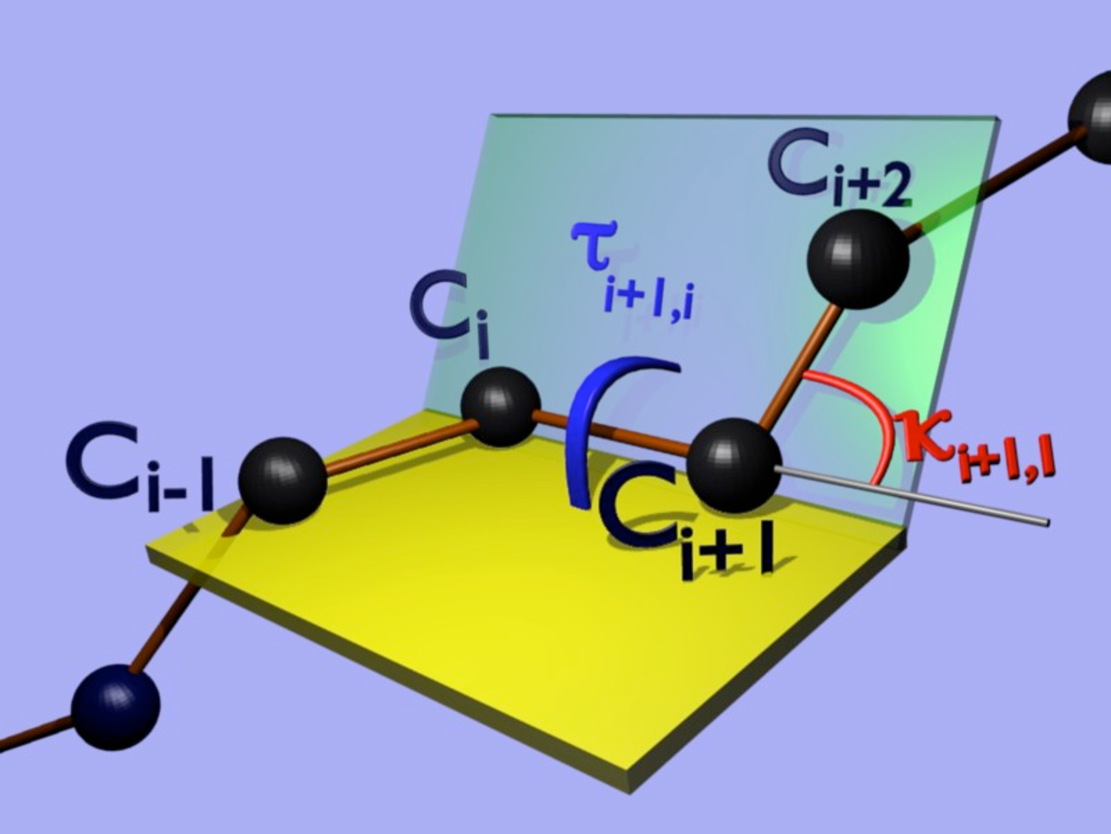
Figure 1: Definition of bond $\kappa$ and torsion $\tau$ angles in terms of the backbone $C_{\alpha}$ carbons.

Note that according to (2), the bond and torsion angles are link variables. In particular, the definition of the bond angle involves three vertices while the definition of the torsion angle involves a total of four vertices.

We have employed the generalized DF equation (2) to inspect the structure of folded proteins. As a data set we have utilized all those proteins that are presently in PDB, with an overall resolution better than 2.0 Ȧngström. There is no additional curation or data pruning. As a control set we have used the highly curated version v3.3 Library of chopped PDB files for representative CATH domains Orengo et al., (1997). Since the conclusions we draw from these two data sets are parallel, we only describe here the results for the first one in detail.

B: Backbone Visualization

We start by describing the visualization of the (frame independent) directions of the tangent vectors $\mathbf{t}_{i}$ along the backbone. For this we note that with the base of $\mathbf{t}_{i}$ at the location of the corresponding $C_{\alpha}$ carbon, its tip determines a point on the surface of a unit two-sphere. The location of this point is described by the bond angle as the latitude, and the torsion angle as the longitude of the two-sphere. Since the $\mathbf{t}_{i}$ are frame independent, the traces of their tips on the two-sphere provides frame independent information of the backbone geometry. For visualization of the two-sphere, we can stereographically project it from south-pole $(\kappa_{i}\equiv\kappa_{i,i+1}=\pi)$ onto the two dimensional plane. This leads us to the angular distributions that we have displayed in Figure 2, and in each of the four classes in this Figure we have used the prevalent PDB identification of the ensuing structures.

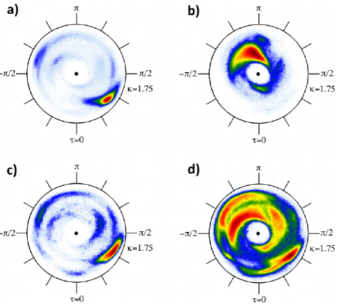
Figure 2: The four major protein structures: a) $\alpha$-helices, b) $\beta$-strands, c) $3/10$-helices and d) loops according to PDB classification in our data set. In each Figure the center of the annulus is the north-pole of the two-sphere where the bond (latitude) angle $\kappa=0$ so that the two consecutive unit tangent vectors $\mathbf{t}_{i}$ and $\mathbf{t}_{i+1}$ are parallel. The bond angle then measures distance from the center of the annulus so that the south pole where $\kappa=\pi$ corresponds to points at infinity on the plane, where $\mathbf{t}_{i}$ and $\mathbf{t}_{i+1}$ become anti-parallel. The torsion i.e. longitude angle $\tau\in[-\pi,\pi]$ increases by $2\pi$ when we go around the center of the annulus in counter-clockwise direction. The color coding in all our Figures increases from white to blue to green to yellow to red and describes the relative number of conformations in PDB in a $\log$-squared scale.

The four maps in Figure 2 portray all the essential features of the Ramachandran map. But there are also important differences that makes it profitable to utilize these maps both in lieu of and in combination with the Ramachandran map. The predominant feature in Figures 2 is that the PDB data is concentrated in an annulus which is located roughly in the range $\kappa\approx(1,\pi/2)$. The exterior of the annulus (roughly $\kappa>\pi/2$) is an excluded region that describes conformations with steric clashes. The interior (roughly $\kappa<1$) is sterically allowed but excluded as long as proteins remain in the collapsed phase; The interior region becomes occupied when we cross the $\Theta$-point and proteins assume their unfolded conformations. The loops also appear to have a slightly higher tendency to bend towards left i.e. $\tau<0$. Note that in the Figures for $\alpha$, $\beta$ and $3/10$ the blue regions correspond to residues whose present PDB classification are not consistent with our computed $(\kappa,\tau)$ values; Such issues have also been raised in Hovmöller et al., (2002).

Moreover, the Figure 2 reveals that the PDB data displays innuendos of various underlying reflection symmetries: In the Figure 2d (loops) there is a clearly visible mirror of the standard right-handed $\alpha$-helix region, located in the vicinity of the outer rim with $\kappa\approx 1.5$ and with torsion angle close to the value $\tau\approx-2\pi/3$. A helix in this regime would be left-handed and tighter than the standard $\alpha$-helix. There is also a clear mirror structure in the Figure 2b for $\beta$ strands, the standard region is $(\kappa,\tau)\approx(1,\pi)$ and its less populated mirror is located around $(\kappa,\tau)\approx(1,0)$. The mirror symmetry between the ensuing extended regions persists in the Figure 2d for loops.

Finally, in the Figure 2d we observe a small elevated (yellow) region in the vicinity of $(\kappa,\tau)\approx(1.5,-\pi/3)$. This is the region of helices that are spatial left-handed mirror images of the standard $\alpha$-helices. There is also a (slightly) elevated (green) mirror of this region around $(\kappa,\tau)\approx(1.5,2\pi/3)$. This is like the $(\kappa,\tau)\approx(1.5\,,-2\pi/3)$ mirror of the standard right-handed $\alpha$ helices.

C: Side-Chain Visualization

In Figure 3 (top) we display the orientations of the $C_{\beta}$ carbons in the Frenet frames of the $C_{\alpha}$ carbons i.e. all $\Delta_{i}=0$ in (1); Recall that a $C_{\beta}$ carbon is present in all non-glycyl residues. In this Figure the $C_{\alpha}$ carbons are at the center of the sphere. Consequently the Figure 3 (top) shows directly the locations of the $C_{\beta}$ carbons as seen by an observer who traverses the $C_{\alpha}$ backbone with a gaze orientation that is determined by the DF frame. We find it remarkable that in this frame the directions of the $C_{\beta}$ carbons are subject to only very small nutations. The additional feature is the presence of the highly localized, isolated island.

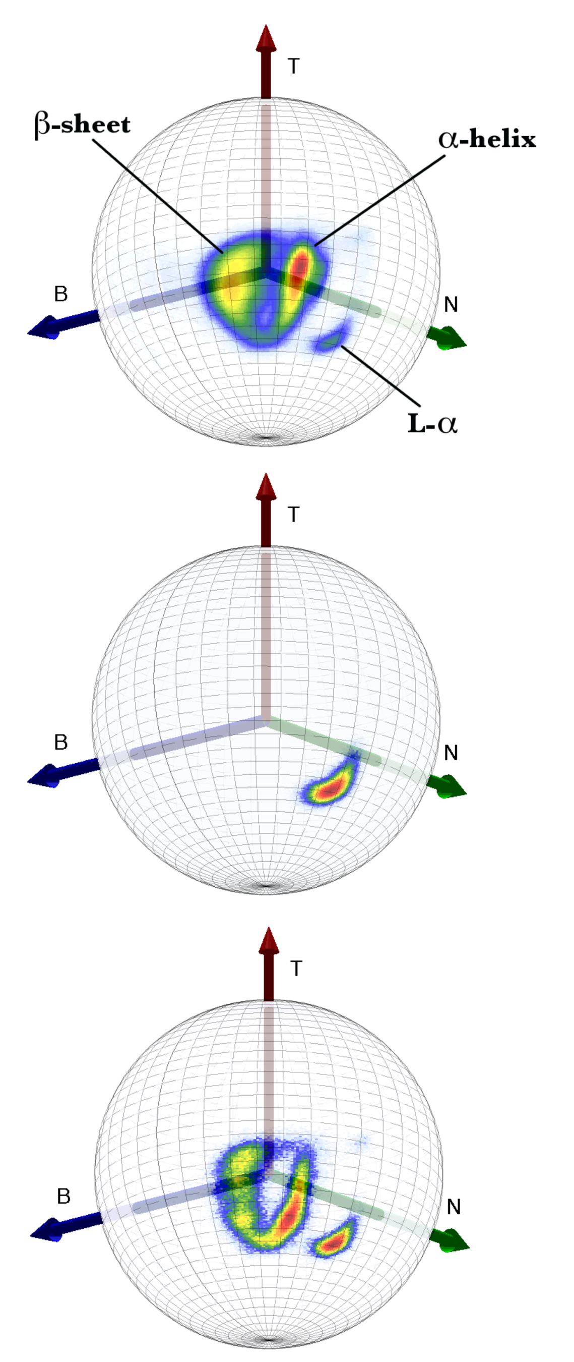
Figure 3: The DF frame directions of the $C_{\beta}$ carbons. On top all residues in our data set including ASN. In the middle we display only the $\tt L$-$\alpha$ region of the Ramachandran map. On bottom we display only those ASN that are in a loop in PDB classification. The color coding is proportional to the ensuing propensity.

Indeed, we have found that for non-glycyl residues this isolated island coincides with the $\tt L$-$\alpha$ region of the Ramachandran map. This is shown in Figure 3 (middle) where we display the direction of the $C_{\beta}$ carbons solely for those residues that are in the $\tt L$-$\alpha$ Ramachandran region. Finally, in the Figure 3 (bottom) we display the DF frame distribution of the $C_{\beta}$ carbons for those ASN that are located in loops only, according to PDB classification. The relatively high propensity of ASN in the $\tt L$-$\alpha$ island is prominent. In the sequel we shall concentrate our attention solely on the isolated $\tt L$-$\alpha$ island in Figure 3 (middle).

Figure 4 describes the propensity of different amino acids in the $\tt L$-$\alpha$ island of Figure 3. This Figure confirms the high propensity of ASN (N) that is already visible in Figure 3 (bottom). We find that ASP (D) has also relatively high propensity. But the propensity of histidine (H) is practically equal in our data. Furthermore, several non-carbonylic amino acids have a higher propensity than GLU (E). The $\beta$-branched isoleucine (I), valine (V) and threorine (T) all have clearly suppressed propensities and proline (P) is practically absent, presumably reflecting the presence of steric constraints Deane et al., (1999), Hovmöller et al., (2002), Chakrabarti et.al.., (2001).

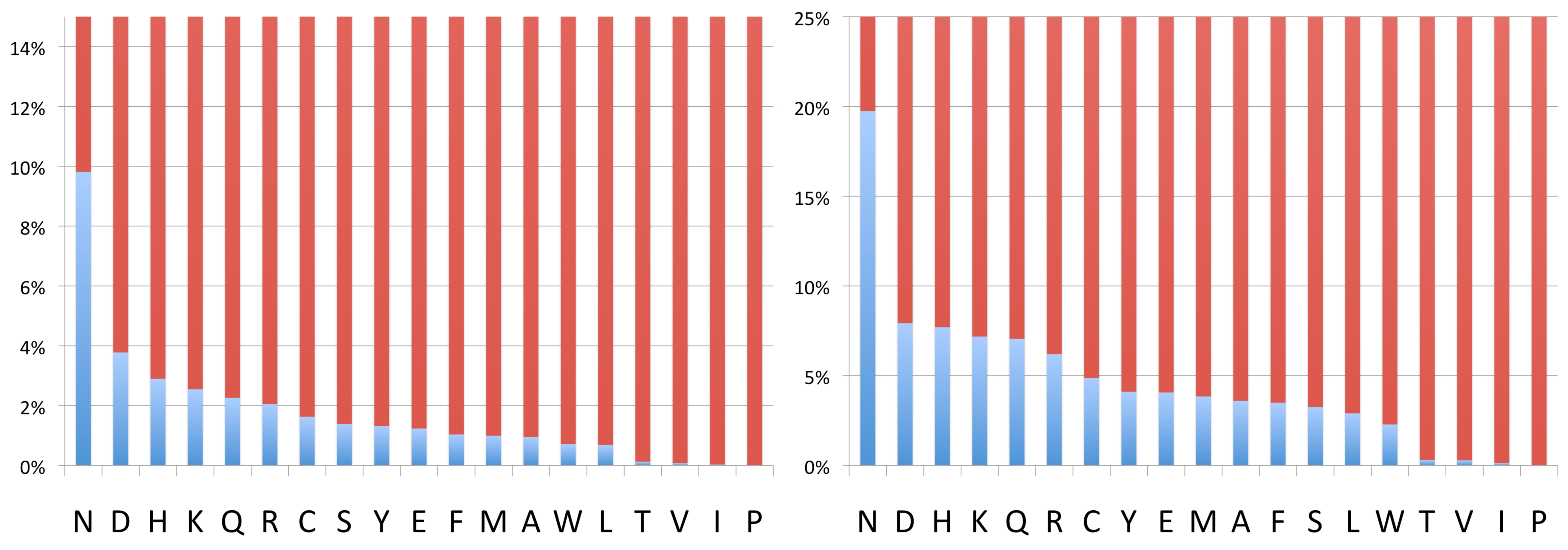
Figure 4: The propensity of non-glycyl residues in the $L$-$\alpha$ island of Figure 3. In the left we display the result for all amino acids in our entire data set, and in the right for those in our data set that are classified as loops in PDB. The propensity of carbonylic ASN (N) is clearly enhanced in both cases. But in both cases the similarly carbonylic ASP (D) has about the same propensity with the non-carbonylic HIS (H), and the carbonylic GLU (E) is relatively quite suppressed.

We have also analyzed the directions of the $C_{\gamma}$ carbons, as seen by a $C_{\alpha}$ observer in the DF frame. The result presented in Figure 5 reveals that at the level of $C_{\gamma}$ the data points in the single $\tt L$-$\alpha$ island of Figure 3 remain highly localized even though it now becomes divided into two separate islands. There is a putative gauche+ ($g$+) island where around 70$\%$ of the residues in the $L$-$\alpha$ island are located, and a putative trans island for the rest; We do not see any putative gauche- region. The amino acid propensities of these two islands is displayed in Figure 6. ASN is the most populous in both $C_{\gamma}$ islands. However, the propensity of ASP is elevated only in trans island. In the g+ island both non-carbonylic HIS (H) and LYS (K) and even the carbonylic GLN (Q) have a higher propensity than ASP.

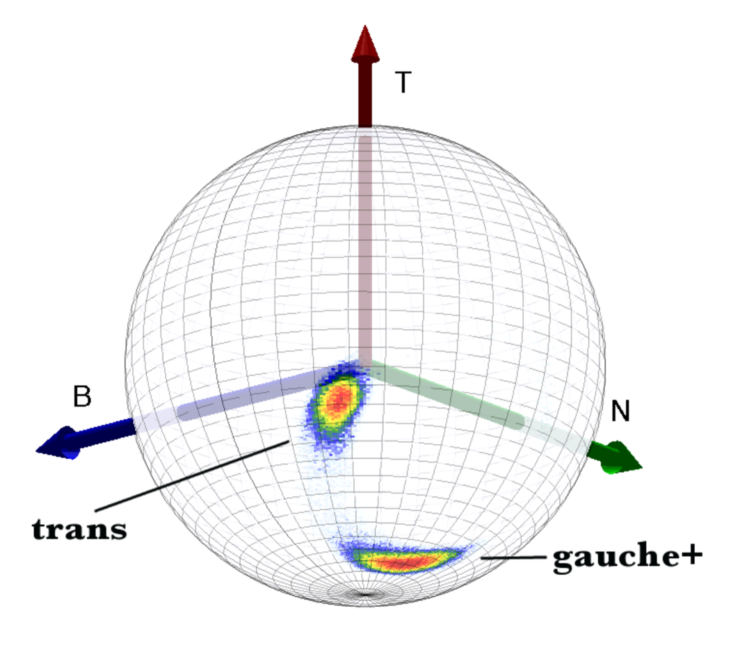
Figure 5: The DF frame directions of $C_{\gamma}$ carbons for residues located in the $\tt L$-$\alpha$ island.

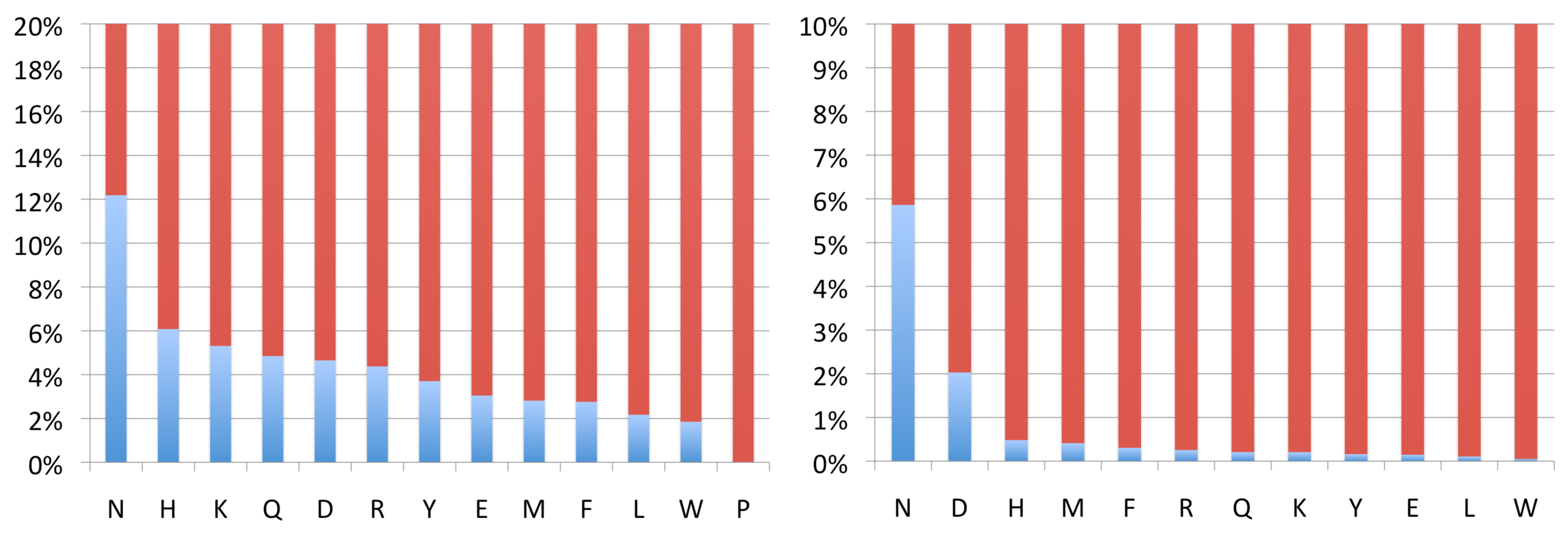
Figure 6: The propensity of different amino acids in the putative g+ island (left) and trans island (right)

In Figure 7 we plot the percentage of different amino acids as they appear in our data set in the two $C_{\gamma}$ islands. Note that around $43\%$ of residues in the putative $\it g+$ island are non-carbonylic, while in the putative $\it trans$ island the number is close to $12\%$.

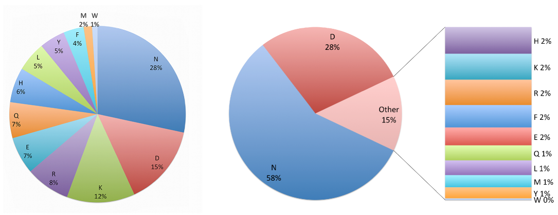
Figure 7: The relative number of different amino acids in the putative $\it g+$ (left) and $\it trans$ (right) $C_{\gamma}$-islands.

In Figure 8 we plot the $C_{\delta}$ carbons in the DF frame of the $C_{\alpha}$ carbons. Since ASN (and ASP) has no $C_{\delta}$ carbon, we display instead the direction of the side-chain $O$ atom for ASN, and the result is shown in Figure 9.

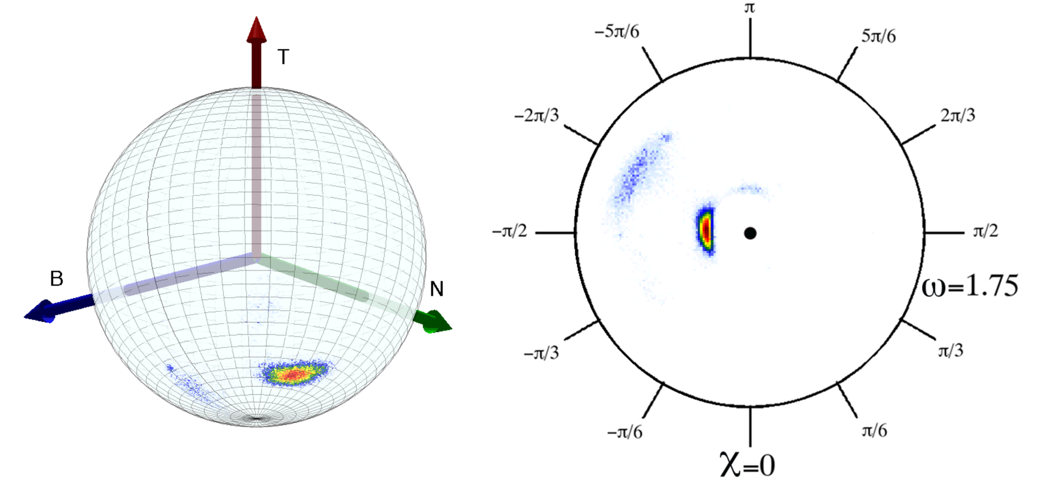
Figure 8: The directions of the $C_{\delta}$-carbons in the DF frame of the $C_{\alpha}$ carbons on the two-sphere (left), and on stereographically projected $C_{\beta}$ frame (right).

From Figure 8 we observe that the directions of the $C_{\delta}$ continue to be highly localized, independently of the type of amino acid. We also observe the formation of a second but relatively weakly occupied island at larger values of the latitude angle and with longitude angle $\chi\sim-2\pi/3$, clearly visible in Figure 8 (right). At the moment we do not have a basis to conclude whether this is a real effect or simply a reflection of problems in the experimental data.

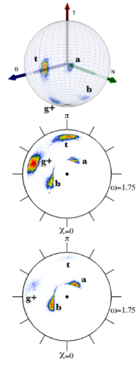
Figure 9: On top, the directions of the side-chain $O$ atoms of ASN in the DF frame of the $C_{\alpha}$ carbons. In the middle, the same as on top but on stereographic projection and in the $C_{\beta}$ frame. Bottom, the directions of the side-chain $N$ atoms of ASN in the same $C_{\beta}$ frame as in middle suggesting that the correct identification of a and b regions in the top and middle figure is $N$. The identifications follow PDB. (t is trans and g+ is gauche+)

In Figure 9 we display the $O$ atoms of the ASN side-chain according to PDB identification in the DF frame of the $C_{\alpha}$-carbons. We note that the two $C_{\gamma}$ islands appear to become divided into four distinct but still highly localized islands. However, it is well known that the identification between the ASN side-chain $O$ and $N$ can be very difficult Weichenberger et al., (2007), and thus we have displayed in Figure 9 (bottom) the $N$ atoms according to PDB identification as well. By comparing the Figures 9 (middle) and (bottom) we conclude that most likely the two inner-most islands denoted a and b in Figure 9 describe $N$ instead of $O$ atoms.

II Results and Discussion

Previously it has been proposed that in the case of ASN and ASP, the $\tt L$-$\alpha$ Ramachandran region is stabilized by a non-covalent attractive interaction between the side-chain and backbone carbonyls Deane et al., (1999), Chakrabarti et.al.., (2001). Here we find that in the DF frame and independently of the amino acid, the ensuing side-chain $C_{\beta}$ carbons all point to the same direction that we have denoted $\tt L$-$\alpha$ in Figure 3. We have shown that this region does also coincide with the non-glycyl $\tt L$-$\alpha$ region of the Ramachandran map. Furthermore, the strong localization in the direction continues to persist when we extend our analysis to the $C_{\gamma}$ and $C_{\delta}$ carbons of the $\tt L$-$\alpha$ residues, the results are displayed in Figures 6 and 9 respectively; In the case of ASN (ASP) where there is no $C_{\delta}$ carbon we utilize the side chain $O$ and $N$ atoms instead and as shown in Figure 10 the results are very similar. This strong localization in the directions and in particular its apparent residue independence suggests that the presence of the $\tt L$-$\alpha$ island is associated with some relatively residue independent structural property of the protein backbone.

According to Deane et al., (1999), in the case of ASN and ASP the backbone oxygen atom has a special rôle. If so, it should somehow be reflected in the ensuing backbone conformations. In order to scrutinize this, we have inspected the orientations of all backbone $O$ atoms in our data set, in a group of residues where the $i^{th}$ one is located in the island. The result is shown in Figure 11: We find that there is a very strong localization in the directions of the backbone $O$ atoms, and this localization is residue independent and extends itself over at least four different residues: The $O$ atoms in both the $\tt L$-$\alpha$ site $i$ and at the preceding site $i-1$ are highly localized into a single direction, while for both the site $i-2$ and the site $i+1$ we identify three closely located directions, that are presumably related to the three available trans/gauche conformations.

Indeed, it appears that only very few backbone geometries are accessible in the vicinity of a residue that is located in the $\tt L$-$\alpha$ island. Furthermore, since the regime that extends from the $(i-2)$nd to the $(i+1)$st site involves three sets of curvature and torsion angles, each of them defined in terms of three resp. four residues we conclude that the backbone geometries reflect the collective interplay of at least up to seven different sites along the backbone.

Figure 10: The orientations of backbone $O$ atoms around the site $i$ that is located in the $\tt L$-$\alpha$ island, in the $C_{\alpha}$ discrete Frenet frame of the $i^{th}$ central $C_{\alpha}$-carbon. For the $i^{th}$ and $(i-1)$st atom only one position appears to be available while the $(i+1)$st and $(1-2)$nd atoms each have three available (trans/gauche) positions. The angle $\phi$ is measured from the $\bf N$ axis.

To further inspect the universality of the $\tt L$-$\alpha$ island, we consider the distribution of the backbone bond and torsion angles that are attached to a $C_{\alpha}$ carbon when a residue is located in the $\tt L$-$\alpha$ island. The result is shown in Figure 11 separately for ASN and ASP, and for the remaining non-glycyl amino acids.

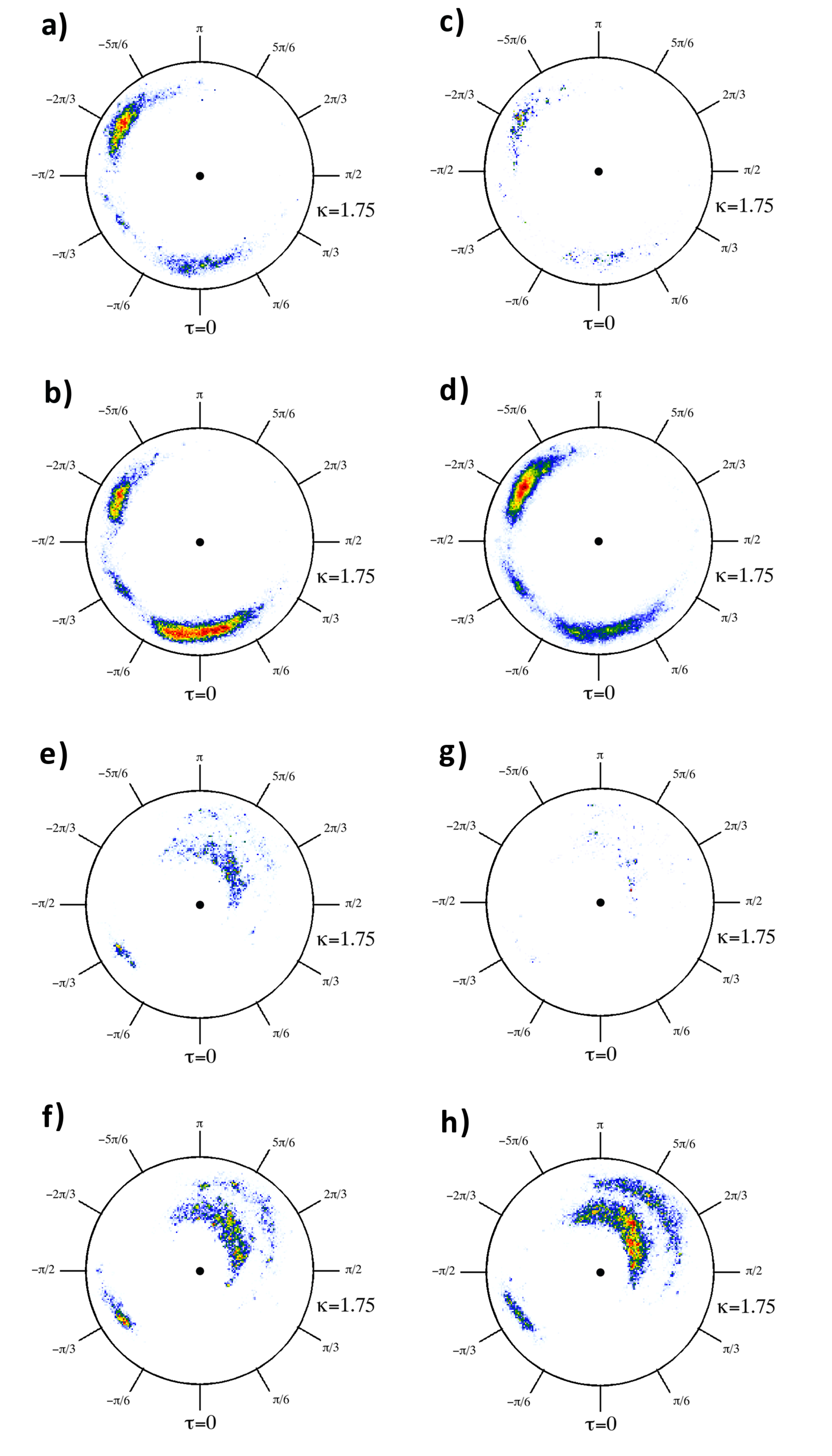
Figure 11: The $(\kappa,\tau)$ distributions for backbone links that are attached to a $C_{\alpha}$ carbon with residue in the $\tt L$-$\alpha$ island. Separately for ASN and ASP, and for the rest. On left column the $C_{\alpha}$ carbons in the case where the corresponding $C_{\gamma}$ carbon is in the trans island, on right for those where the $C_{\gamma}$ is in the $g$+ island. First row is for link that precedes either ASN or ASP. Second row is for link preceding any other non-glycyl amino acid. Third row is for link following either ASN or ASP. Fourth row is for link following the others.

We find no essential difference between the different residues, nor do we find any essential difference between the trans and $g$+ islands. Moreover, we observe the following general pattern: For the backbone $C_{\alpha}$ link that precedes the $\tt L$-$\alpha$ island, three different regions on the $(\kappa,\tau)$ plane are probable. These are the regions that we have denoted with a, b and c respectively in the Figure 12-left; In this Figure we have combined all the data that are displayed separately in the parts a, b, c and d of Figure 11. After the $\tt L$-$\alpha$ island there are also three different regions that are probable. We denote these regions with letters b and d and e respectively in the Figure 12-right, now combining the data in parts e, f, g, h in Figure 11. Note that the regions b in the two parts of Figure 12 practically coincide.

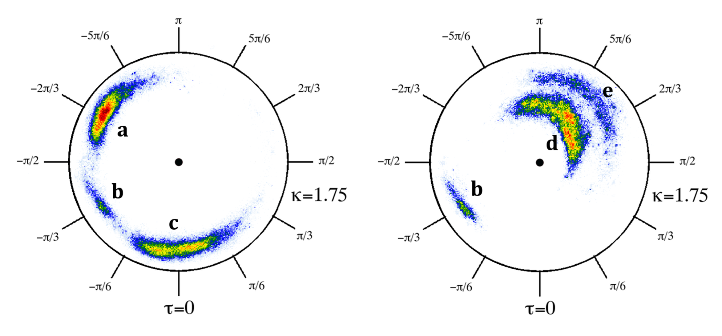
Figure 12: The $(\kappa,\tau)$ distributions for all backbone links that are attached to a residue in the $\tt L$-$\alpha$ island. On the left for the link preceding the residue in the $\tt L$-$\alpha$ island, on the right following the residue in the $\tt L$-$\alpha$ island.

By inspecting the protein structures in our data set we conclude that the presence of a residue in the $\tt L$-$\alpha$ island causes the following phenomenologically verified selection rules in Figure 12:

$\bullet$ The region a can only precede regions d and e.

$\bullet$ Both regions b and c can be followed by any of the three regions

b, d and e.

Furthermore, we find that

$\bullet$ The residue preceding either a or c is not located in the $\tt L$-$\alpha$

island.

$\bullet$ Both the residue preceding and following b can be located in

the $\tt L$-$\alpha$ island.

$\bullet$ If the two residues following c are both in the $\tt L$-$\alpha$ island, the

first residue connects c to b and the second connects b to b.

We remind that since the region b has the same curvature angle as the standard $\alpha$-helix region and since the torsion angles are equal in magnitude but have an opposite sign, a repeated structure in b is the right-handed mirror image of the standard $\alpha$-helix, this is truly the region of left-handed $\alpha$-helices.

We have also found that there appears to be four main trajectories that are followed by the orientations of those $C_{\alpha}$ carbons that surround a residue located in the $\tt L$-$\alpha$ island. The result is shown in the schematic Figure 13, where the pink arrows correspond to residues in the island; Recall that the curvature and torsion angles are link variables, they connect two $C_{\alpha}$ carbons according to (2).

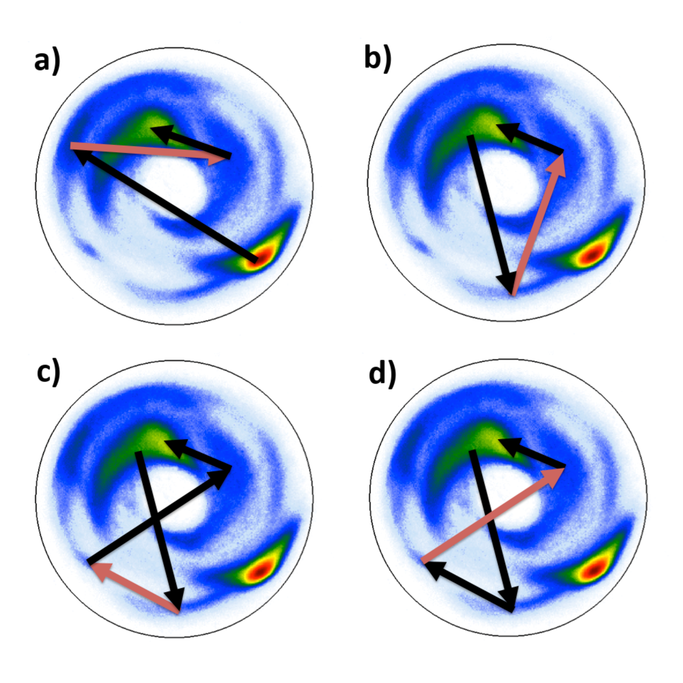
Figure 13: Four different trajectories through a residue in the $\tt L$-$\alpha$ island that are common in our data set. In each case the pink lines denotes the transition caused by the residue in the $\tt L$-$\alpha$ island. The trajectory a described a turn from $\alpha$-helix region to $\beta$-strand region, and the remaining ones start and end in the $\beta$ region; these include $\beta$-turns.

In Figure 13a, the first residue takes us away from an $\alpha$-helix region to the region a in the Figure 12 left (black arrow). This is followed by a residue in the $\tt L$-$\alpha$ island, that takes us to the region d in the Figure 12 right (pink arrow). Finally, there is a transition to the $\beta$-strand region (black arrow).

The second trajectory in Figure 13b starts from the $\beta$-strand region with a residue that takes it into region c in Figure 12 left. The following residue that is located in the $\tt L$-$\alpha$ island then causes a transition into region d in Figure 12 right (pink arrow). This is followed by a transition back to a $\beta$-strand region.

The third trajectory that we have described in Figure 13c starts from the $\beta$-strand region and proceeds to region c in Figure 12 left. From there the trajectory proceeds to region b in Figure 12 left, with the transition caused by a residue in the $\tt L$-$\alpha$ island. This is followed by a transition to region d and then back to the $\beta$-strand region.

Finally, the fourth trajectory that is also common in our data set is the one displayed in Figure 13d. It is similar with the trajectory described in Figure 13c, except that now the residue that is located in $\tt L$-$\alpha$ island causes the transition from b to d in Figure 12.

The Figures 12 and 13 reveal that the presence of a residue in the $\tt L$-$\alpha$ island relates to a collective topology of the backbone involving several residues. Since the definition of a bond angle takes three $C_{\alpha}$ carbons and the definition of a torsion angle takes four (see Figure 1), we conclude that the topology of the trajectories in Figures 13a and 13b involve the interplay of seven residues while in 13c and 13d there are a total of eight residues present.

Finally, we have verified that all our results are independent of the data set we have used by similarly analyzing the proteins in the version v3.3 Library of chopped PDB files for representative CATH domains. The results are very similar. But in addition, we find that the propensity is largest in the (mainly-$\beta$) CA level classes 2.90, 2.160 where over 5$\%$ of all residues are in the island. We also find that any CA level family has at least 1$\%$ of their residues in the island, except 1.40 where the single representative with PDB code 1PPR has no residues in the island.

III Conclusion

We have investigated the non-glycyl residues that are located in the $\tt L$-$\alpha$ region of the Ramachandran map. Independently of the amino acid, we find that in the Discrete Frenet frames of the $C_{\alpha}$ carbons the corresponding side-chain $C_{\beta}$ carbons are localized in the same direction. This universality in the orientation persists when we investigate the $C_{\gamma}$ and $C_{\delta}$ carbons, the side chain $O$ and $N$ atom in the case of ASN and ASP. The results suggest that instead of reflecting only a local interaction between a given backbone unit and its residue, the $\tt L$-$\alpha$ island is associated with a largely residue independent backbone conformation that involves the collective interplay between several consecutive residues.

When we proceed to analyze the distribution of those backbone bond and torsion angles that are associated with the links that both precede and follow a residue that is located in the $\tt L$-$\alpha$ island, we find that independently of the residue these angles display very similar patterns. Since the definition of a bond angle takes three $C_{\alpha}$ carbons and the definition of a torsion angle takes four, this prompts us to propose that the geometrical structure associated with the presence of a residue in the $\tt L$-$\alpha$ island reflects the interplay of at least seven consecutive backbone units. In particular, we have not been able to pin-point any obvious local reason (charged, polar, acidic, hydrophobic/philic) to explain the presence or absence of a residue on the $\tt L$-$\alpha$ region.

Our approach is based on a novel method to depict proteins. In the course of our analysis we have been able to observe several systematic patterns including anomalies in the PDB data, suggesting that the method we have utilized has a potential of becoming a valuable tool for both experimental and theoretical protein structure analysis and fold prediction.

References

- Ramachandran et al., (1963) Ramachandran, G.N., Raakrishnan, C and Sasisekharan, V. (1963), Stereochemistry of polypeptide chain configurations Journal of Molecular Biolology 7 95 99
- Hovmöller et al., (2002) Hovmöller, S., Zhou, T., and Ohlson, T. (2002) Conformations of amino acids in proteins Acta Crystallographica D58 768 776
- Deane et al., (1999) Deane, C.M., Allen, F.H., Taylor, R. and Blundell, T.L. (1999) Carbonyl-carbonyl interactions stabilize the partially allowed Ramachandran conformations of asparagine and aspartic acid, Protein Engineering 12 1025-1028
- Allen et al., (1998) Allen, F.H., Baalham, C.A., Lommerse, J.O.M. and Raithby, P.R. (1998) Carbonyl-carbonyl Interactions can be Competitive with Hydrogen Bonds Acta Crystallographia B54 320-329
- Chakrabarti et.al.., (2001) Chakrabarti, P. and Pal, D. (2001) The interrelationships of side-chain and main-chain conformations in proteins Progress in Biophysics & Molecular Biology 76 1-102
- Robinson et al., (2001) Robinson, N.E. and Robinson, A.B. (2001) Deamidation of human proteins, Proceedings of National Academy of Sciences USA 98 12409 12414.
- McCuddena et al., (2006) McCuddena, C.R. and Kraus, V.B. (2006) Clinical Biochemistry 39 1112-1130
- Koo et al., (1999) Koo, E.H., Lansbury, P.T. and Kelly, J.W. (1999) Proceedings of National Academy of Sciences USA 96 9989-9990
- Robinson et al., (2004) Robinson, N.E. and Robinson, A. B. (2004) Molecular Clocks Deamidation of Asparaginyl and Glutaminyl Residues in Peptides and Proteins Althouse Press (London)
- Hu et al., (2011) Hu, S., Lundgren, M. and Niemi,A.J. (2011) e-print arXiv:1102.5658v1 [q-bio.BM]
- Hanson, (2006) Hanson, A.J. (2006) Visualizing Quaternions, Morgan Kaufmann Elsevier (London)
- Kuipers, (1999) Kuipers, J.B. (1999) Quaternions and Rotation Sequences: a Primer with Applications to Orbits, Aerospace, and Virtual Reality, Princeton University Press (Princeton)
- Bishop, (1974) Bishop, R.L. (1974) There is more than one way to frame a curve Americal Mathematical Monthly 82 246-251
- Hartenberg et al., (1964) Hartenberg R.S. and Denavit, J. (1964) Kinematic synthesis of linkages (McGraw-Hill, New York, NY, 1964)
- Faddeev et al., (1986) L. Faddeev, L and Takhtajan, L. (1986) Hamiltonian methods in the theory of solitons Springer-Verlag (Berlin)
- Berman et al., (2007) Berman, H.M., Henrick, K., Nakamura, H., J.L. Markley, J.L., (2007) The Worldwide Protein Data Bank (wwPDB): Ensuring a single, uniform archive of PDB data. Nucleic Acids Research 35, (Database issue) D301
- Orengo et al., (1997) Orengo, C.A., Michie, A.D., Jones, S., Jones, D.T., Swindells, M.B., Thornton, J.M. (1997). CATH–a hierarchic classification of protein domain structures, Structure 5, 1093 1108.
- Weichenberger et al., (2007) Weichenberger, C.X. and Sippl, M.J. (2007) NQ-Flipper: recognition and correction of erroneous asparagine and glutamine side-chain rotamers in protein structures, Nucleic Acids Research 35 (Web Server Issue) W403-406