Experimental Investigation of Forecasting Methods Based on Universal Measures

Abstract

We describe and experimentally investigate a method to construct forecasting algorithms for stationary and ergodic processes based on universal measures (or so-called universal data compressors). Using some geophysical and economical time series as examples, we show that the precision of thus obtained predictions is higher than that of known methods.

1 Introduction

The problem of forecasting is important for many applications. Nowadays there are many efficient forecasting methods, which are based on different approaches and different mathematical models (see for review, for ex., De Gooijer & Hyndman (2006) and Makridakis (1996)). Many such approaches are deeply connected with different ideas and results of mathematical statistics, probability theory and some other fields.

In this paper we develop and experimentally investigate an efficiency of prediction methods which are based on so-called universal measures (or universal data compressors).

By definition, universal codes, or universal methods of lossless data compression, are intended to “compress” texts, i.e. encode them in such a way that the length of an encoded text is shorter than the length of the initial one (and, of course, the original text can be recovered from the encoded one). It is important that the text statistics is unknown beforehand, that is why such codes are called universal. In fact, universal codes implicitly estimate unknown characteristics of the processes and use them for data compression.

A universal code is called optimal if it encodes a sequence of letters generated by a finite-alphabet source in such a way that the length of the encoded sequence is asymptotically minimal. First universal codes, which are optimal for i.i.d. information sources, were discovered by Fitingoff (1966) and Kolmogorov (1965). The universal codes for stationary and ergodic sources with finite alphabets have been known since 1980’s; see Ryabko (1984).

It is clear that universal codes can be considered as a tool of mathematical statistics and it is natural to try to apply them for solving traditional problems of this science (like hypothesis testing, parameter estimation, etc.) First it was recognized in 1980’s (see Rissanen(1984) and Ryabko(1984, 1988) ) and nowadays it is shown that the universal codes can be efficiently used for hypothesis testing, parameter estimation and prediction of time series with finite and real-valued alphabets; see Ryabko & Astola (2006), Ryabko (2009). However, there are only preliminary results which concern practical applications of prediction methods to real data, see Ryabko & Monarev (2005). These results were rather aimed to illustrate the possibility of such applications than give information about the precision of the methods.

The goal of this work is the construction, implementation and experimental estimation of the methods of prediction suggested, which are based on universal codes and so-called universal measures. To this aim, we have considered several types of time-series data: the indices of solar activity (SA), water level, and cross-rates of some currencies. It is clear that such processes are of great theoretical and practical importance. For example, nowadays the statistical connections between climate and SA are widely investigated.

The obtained experimental results show that the forecasting methods based on universal codes possess a high precision. In principle, any universal code can be used as a basis of a prediction method, but here we use a universal code suggested by Ryabko (1984), which have some additional useful properties, see Krichevsky (1993), Ryabko, Astola (2006).

The outline of the paper is as follows. The next part contains necessary definitions and some information about universal codes and measures. The part three is devoted to prediction of real time series and the part four is a short conclusion.

2 Method and its implementation description

2.1 Description of the method

Here we will describe the forecasting method studied, and also provide required theoretical information. It will be convenient at first to describe briefly the prediction problem. We consider a stationary and ergodic source which generates sequences $x_{1}x_{2}...$ of elements (letters) from some set (alphabet) $A$, which is either finite or real-valued. It is supposed that the probability distribution (or distribution of limiting probabilities) $P(x_{1}=a_{i_{1}},x_{2}=a_{i_{2}},...,x_{t}=a_{i_{t}})$ (or the density $p(x_{1},x_{2},...,x_{t})$) is unknown. Let the source generate a message $x_{1},...x_{t-1}x_{t}$ , $x_{i}\in A$ for all $i$, and the next letter needs to be predicted. Now let us describe the forecasting method. First we define a universal measure and then explain how it is connected with universal codes. By definition a measure $\mu$ is universal if for any stationary and ergodic source $P$ the following equalities are valid:

$$\lim_{t\rightarrow\infty}\,t^{-1}(\log P(x_{1}...x_{t})-(\log\mu(x_{1}...x_{t})))=0,$$

with probability 1, and

$$\lim_{t\rightarrow\infty}\,t^{-1}\sum_{u\in A^{t}}P(u)\log(P(u)/\mu(u)))=0.$$

(Here and below $\log x=\log_{2}x$.) These equations show that, in a certain sense, the measure $\mu$ is an estimate of (unknown) measure $P$. That is why the universal measures can be used for estimation of process characteristics and prediction.

In what follows, we will directly describe a certain universal measure which will be used for prediction in this paper and, in principle, we do not have to mention universal codes at all. But the point is that universal measures are deeply connected with the universal codes and, if one has a universal code, one can simply convert it into a universal measure. It is important for practical applications, because many universal codes are available as computer programs (so-called archivers) and, hence, they can be transformed into universal codes and then directly used for prediction, as it is shown by Ryabko & Monarev (2005). So, we give a short informal definition of universal codes, whereas a full description can be found, for ex., in Ryabko (2010).

Roughly speaking, a code maps words from the set $A^{t}$, $t\geq 1$, into the set of words over alphabet $\{0,1\}$. By definition, a code $U$ is universal (for the set of stationary ergodic sources), if for any stationary and ergodic source $P$ the following equalities are valid:

$$\lim_{t\rightarrow\infty}\,|U(x_{1}...x_{t})|/t=H(P)$$

with probability 1, and

$$\lim_{t\rightarrow\infty}\,|E_{P}(U(x_{1}...x_{t})|)/t=H(P),$$

where $|v|$ is the length of the word $v$, $E_{P}(f)$ is the mean of $f$ with respect to $P$, $H(P)$ is the Shannon entropy of $P$, i.e.

$$H(P)=\lim_{t\rightarrow\infty}\,-\,t^{-1}\,\sum_{u\in A^{t}}P(u)\log(P(u)),$$

Gallager (1968). The following statement shows that any universal code determines a universal measure.

Theorem 1.

Let $U$ be a universal code and

$$\mu_{U}(w)=2^{-|U(w)|}/\sum_{u\in A^{|w|}}\mu_{U}(u).$$

Then $\mu_{U}$ is a universal measure.

(The simple proof of this theorem can be found in Ryabko, (2010).) So, we can see that, in a certain sense, the measure $\mu_{U}$ is a consistent (nonparametric) estimate of the (unknown) measure $P$.

Now we a going to describe the universal measure $R$ which will be used as a basis for forecasting in this paper. For this purpose we first describe the Krichevsky measure $K_{m}$, which is universal for the set of Markov sources of memory, or connectivity, $m$, $m\leq 0$, if $m=0$, the source is i.i.d. In a certain sense this measure is optimal for this set (see for details Krichevsky (1993), Ryabko, (2010).) By definition,

$$K_{m}(x_{1}...x_{t})=\cases{\frac{1}{|A|^{t}},&if $t\leq m\,$;\cr&\cr\frac{1}{|A|^{m}}\>(\frac{\Gamma(|A|/2)}{\Gamma(1/2)^{|A|}})^{|A|^{m}}\prod_{v\in A^{m}}\frac{\prod_{a\in A}\>(\Gamma(\nu_{x}(va)+1/2)}{(\Gamma(\bar{\nu}_{x}(v)+|A|/2))},&if $t>m$ \, ,}$$ (1)

where $x=x_{1}...x_{t},$ $\nu_{x}(v)$ is the count of word $v$ , occurring in the sequence $x_{1}...x_{|v|},$ $x_{2}...x_{|v|+1},$ $...,$ $x_{t-|v|+1}...$ $x_{t}$, $\bar{\nu}_{x}(v)=\sum_{a\in A}\nu_{x}(va)$, $\Gamma()$ is the gamma function.

We also define a probability distribution $\{\omega=\omega_{1},\omega_{2},...\}$ on integers $\{1,2,...\}$ by

$$\omega_{1}=1-1/\log 3,\>...\,,\>\omega_{i}\,=1/\log(i+1)-1/\log(i+2),\>...\;,$$ (2)

$i=1,2,...\,.$ (In what follows we will use this distribution, but the theorem described below is true for any distribution with nonzero probabilities.)

The measure $R$ is defined as follows

$$R(x_{1}...x_{t})=\sum_{i=0}^{\infty}\omega_{i+1}K_{i}(x_{1}...x_{t})\,.$$ (3)

It is important to note that the measure $R$ is a universal measure for the class of all stationary and ergodic processes with a finite alphabet; Ryabko (1984). Hence, $R$ can be used as a consistent estimator of probabilities.

Let us describe the scheme of the forecasting method based on the measure $R$ for the sequences generated by the sources of different types.

2.2 Finite-alphabet case

As we mentioned above the measure $R$ can be applied for prediction. More precisely we may use $R$ for defining the following conditional probability as:

$$R(a|x_{1}...x_{t})=R(x_{1}...x_{t}a)/R(x_{1}...x_{t})\,,$$

$a\in A$. In the finite-alphabet case the scheme of the prediction algorithm is quite simple. Let $x_{1}...x_{t}$ be a given sequence. For each $a\in A$ we construct the sequence $x_{1}...x_{t}a$ and compute the value $R(a|x_{1}...x_{t})$ . Having the set of such conditional probabilities we use them as estimations of the unknown probabilities $P(a|x_{1}...x_{t})$, $a\in A$.

2.3 Real-valued case

Let $(\Omega,F,P)$ be a probability space and let $X_{1},X_{2},...$ be a stochastic process with each $X_{t}$ taking values in a standard Borel space. Suppose that the joint distribution $P_{n}$ for $(X_{1},X_{2},...,X_{n})$ has a probability density function $p(x_{1}x_{2}...x_{n})$ with respect to the Lebesgue measure $L$. (A more general case is considered by Ryabko (2009). In particular, it is shown that any universal measure can be used instead of $R$.) Let $\Pi_{n}$, $n\geq 1$ , be an increasing sequence of finite partitions $\Omega$ that asymptotically generates the Borel sigma-field $F$, and let $x^{[k]}$ denote the element of $\Pi_{k}$ that contains the point $x$. For integers $s$ and $n$ we define the following approximation of the density:

$$p^{s}(x_{1},...,x_{n})=P(x_{1}^{[s]},...,x_{n}^{[s]})/L(x_{1}^{[s]},...,x_{n}^{[s]})\,.$$

Now we define the corresponding density $r$ as follows:

$$r(x_{1}...x_{t})=\sum_{s=1}^{\infty}\omega_{s}R(x_{1}^{[s]},...,x_{t}^{[s]})/L(x_{1}^{[s]},...,x_{t}^{[s]}))$$ (4)

It is shown by Ryabko (2009) that the density $r(x_{1}...x_{t})$ estimates the unknown density $p(x_{1},...,x_{t})$ , and the conditional density

$$r(a|x_{1}...x_{t})=r(x_{1}...x_{t}a)/r(x_{1}...x_{t})$$ (5)

is a reasonable estimation of $p(a|x_{1}...x_{t})$.

In practical application of this method we may face a question about choosing the length of the input data to be considered. One may think that the best result will be achieved when using the maximally available quantity of known time series elements. However, it is not always true, because actually statistical characteristics of the process may vary in time (or the process may have a large memory), and then “old” data contain no information on “new” statistical characteristics. So, if the answer is not obvious, to estimate the probability one should use $\bar{r}$ measure defined below. Let $x_{1}...x_{t}$ be a given sequence. Consider next a set of distinct natural numbers $N$. For each $n$ from $N$ consider the sample $x_{t-n+1}...x_{t}$. In other words, in fact, each sample consists of $n$ last elements of the original time series. Each sample taken individually will be called a “window” with appropriate $n$ as its size. Suppose $N=$ $\{n_{1},...,n_{k}\}$, $k\geq 1$, then

$$\bar{r}(x_{1}...x_{t})=\sum_{i=1}\bar{\omega}_{i}r(x_{t-n_{i}+1}...x_{t})$$

where $\bar{\omega}_{1},\bar{\omega}_{2},$ $...,\bar{\omega}_{k}$ is a probability distribution on $N=\{n_{1},...,n_{k}\}$. (In our calculations we use the following distribution: $\bar{\omega}_{i}=\omega_{i},$ $i=1,...,k-1$ from (2), and $\bar{\omega}_{k}=1/\log(k+1)$.) As well as $r$ we may use $\bar{r}$ for estimation of conditional probability $p(a|x_{1}...x_{t})$. As seen from the definition, $\bar{r}$ is a “mixture” of probabilities for the appropriate time series of different lengths. Thus estimations based on $\bar{r}$ seem to automatically provide close to optimal results in the context of usage simplicity and precision of forecast. In what follows, such way of calculations will be called adaptive mode.

It is worth noting, that such a “mixture” was already used several times in this work (see (3) and (4) ). The point is that the performance of such “mixtures” is close to the performance of the best summand (see details and theoretical justification in (Ryabko, 2010).

2.4 Implementation of the method

Consider next some aspects of the implementation of the investigated method. Suppose there is a certain source which generates values from some real-valued interval $[A;B]$ and we have time series $x_{1}...x_{t}$ generated by this source. The next value $x_{t+1}$ needs to be predicted. For the purpose of simplicity we will consider computations based on $r$. The case of $\bar{r}$ is analogous.

Step 1. Calculate $r(x_{1}...x_{t})$ using (4). We will describe this step in more details. Divide the interval $[A;B]$ into two equal partitions, called bins, and transform $x_{1}...x_{t}$ into a sequence of symbols each of which is equal to the index of the bin, that contains the appropriate point $x_{i}$. (I.e. if 0 and 1 are the bins indexes, we will then obtain from $x_{1}...x_{t}$ the sequence consisting only of these symbols). Then calculate the first item of the sum from the formula (4). As the value of $L$ we take a product of lengths of all buckets containing $x_{i}$ , and the measure $R$ is computed for the sequence obtained as a result of transforming $x_{1}...x_{t}$ for the current quantization. After that again we divide each of the existing bins (there are two) into two equal bins (there will be four) and for this new quantization do analogous operations to compute the second term from the right-hand side of the equation (4). Go on in this way until getting the quantization for which each of the distinct time series values (including those added at the next step) belongs to distinct bins. Summing all terms, obtain $r(x_{1}...x_{t})$ from (4). It should me mentioned that at this step any other algorithm for achieving the increasing sequence of finite partitions of $[A;B]$ may be applied.

Step 2. Consider the set $P$ consisting of points $A$,$A+h$, $A+2h,$ $...,B$ , where $h$ is a certain small constant. (In this paper $h=0.01$ was used.) For each element $a$ of this set we construct the sequence $x_{1}...x_{t}a$ and compute the value $r(x_{1}...x_{t}a)$ similarly. Here we use the quantizing that is the same as for previous step. Then by formula (5) for each element from the set $P$ calculate the estimations of the appropriate conditional probabilities and find the corresponding prediction. In this paper the forecast value was considered to be equal to the element from $P$ with the biggest estimate of conditional probability. But any other adequate approach may be used.

3 Experimental results

In this section the results of experimental estimation of the method, described in the previous section, are given. All the processes investigated had values from the corresponding interval. To have a possibility to compare the results obtained by the investigated method, with the corresponding actual values, all time series values used in the experiments were taken from the past. The computations in this section can be divided into the two independent parts. In the first part we considered only the forecasting method, while in the second part some preprocessing was used. The detailed descriptions of the computations, along with the results of these experiments are given below, in the corresponding subsections.

Simple time series forecasting. As the target here we chose the time series consisting of the following indices: monthly and smoothed monthly means of sunspot numbers, absolute daily and monthly solar flux values. All datasets used in the experiments of this subsection, can be found at the National Geophysical Data Center (NGDC) Internet site in the “Space Weather $\&$ Solar Events” section. This subsection includes the study of two items.

One-step ahead forecasting. The content of each experiment can be described as follows. Given $t$ successive values of certain time series, we tried to forecast its $(t+1)$th element. For the purpose of the analysis of connection between the known values and the forecast precision for each process the time series with different lengths were considered. Moreover, in order to explore the possibility of computational optimization, additional calculation in adaptive mode was carried out. (See previous section for this method details). We should mention here, that the set of “window” sizes for each process in this case was the same as that consisting of all length used for this time series during the calculations without the “window”, and each item of the sum was equiprobable in the “mixture”. For each length of the time series related to a certain process, and also for the corresponding calculations in adaptive mode, there were 25 experiments on independent datasets. After doing all appropriate computations, the precision estimation was made by considering the differences between the forecast and actual values. The results of the experimental computations of this stage are given in Table 1 below. The first column contains the name of the investigated time series, the second gives the range of its values. The rest of the columns contain the mean absolute error (MAE), obtained either in the calculations in the adaptive mode, or when using the corresponding length of the time series. The “n/d” (“no data”) text means that no calculations were carried out, because there was no data. For example, the information in the third row of the table indicates that for the time series on absolute daily solar flux the MAE corresponding to the calculations based on the 4000 known values, is 1.45. All time series values belong to the range [50; 300]. Also, taking into account the first row of the table, we may say that for the monthly sunspot numbers data the MAE for calculations in adaptive mode, using the “window” with sizes $500,700,1000,1200,2000$ and $3000$, is $23.97$.

Table 1: Experimental computations results of the subsection 3.1

Time series	Range	Adapt.	Length
			500	700	1000	1200	2000	3000	4000
Monthly sunspot number means	[0; 256]	23,97	6,54	2,56	9,58	15,85	21,7	19,63	n/d
Smoothed monthly sunspot number means	[0;210]	2,34	1,5	1,1	1,99	0,77	3,36	2,56	n/d
Absolute daily solar flux	[50;300]	1,78	1,17	1,17	2,71	5,52	8,35	1,72	1,45
Absolute monthly solar flux	[580;2540]	45,29	211,29	45,88	2,71	n/d	n/d	n/d	n/d

Short-dated forecasts comparison.   Here we compared the short-dated forecast for smoothed sunspot numbers, which was published at the NGDC site, with that obtained from the method based on $R$ measure. According to the information, provided at the NGDC site today there exists a special forecasting software (in what follows - NGDC software), which forms a “preliminary look” at the current solar cycle using the improved McNish-Lincoln method. In accordance with the information published on the server, NGDC software constructs the forecast for smoothed monthly sunspot number means and also uses the known values of the time series elements for the certain process. As the NGDC software forecast the file sunspot.predict of 06.08.2008 published on the site was taken, where for each month of the current solar cycle the corresponding forecast value and its confidence interval are given. We should note here that in our comparison we considered just the forecast value, without taking into the account the confidence interval. It is known that at the forecast producing moment for the process there were available and consequently usable data up to February, 2008. Hence, at the computations carrying out moment in June of 2010 there were 21 already known values of the investigated time series (for each month from March, 2008 till November, 2009). Computations by the explored method without “window” usage were carried out according to the following scheme. At first, we point out the time series having the defined length within the certain experiment and with its last element related to February, 2008. Basing on the sequence, we get the one-step ahead forecast, i.e. prediction on March, 2009. Then, at the next iteration we shift the borders of the time series with known values to the right on the one position, replacing the new last sequence element (related to the actual value of March, 2009) with the forecast value obtained at the previous iteration. Basing on this changed time series, we again get the one step ahead forecast, on April, 2008. And so on. Finally, for each observed length of time series 21 experimental computations were carried out. The last forecast value was achieved for November, 2009. The calculations in adaptive mode were accomplished in a similar way but with observing the set of time series of different lengths at the each iteration instead of considering one time series. Likewise in the previous item, the set of “window” sizes for each process in this case was the same as that, consisting of all lengths used for this time series during the calculations without the “window”, and each item of the sum was equiprobable in “mixture”. After the accomplishing of all appropriate computations, the precision estimation was made by considering the differences between corresponding forecast and actual values. The results of experimental computations for the investigated method are placed in Table 2. The first row contains MAE for $R$ measure based method and the appropriate input data. The second row includes MAE for computations, applying the NGDC software. So, it is seen, from the table that for the forecast using the described method and the time series of size 1000 the MAE is 1.87 for 21 experiments. For the NGDC software this value was calculated on the basis of one forecast file.

For illustration purposes the results obtained at this stage of experimental estimation are shown at the Fig. 1 below. At the graphic $N$ axis is the smoothed monthly sunspot numbers and $t$ axis presents the time units with each related to the certain month of the solar cycle. The part of the graphic with $t\leq 0$ is the period with data for forecast producing, and the part with $1\leq t\leq 21$ is the period of time for which the forecasts were made. The solid bold line displays the actual process values (note that they are from the end of time series only), and the dashed lines with short and long dashes plot the forecast values achieved by NGDC software and by the method based on $R$ measure in adaptive mode correspondingly. In the case of using NGDC software the comparable MAE was observed only for the first four forecast values and was 1.95. After the ten experiments it was growing up to 5.51 and, finally, after all 21 computations of this number of experiments the value equaled 16.39. So, we may say, that there was obvious trend of the MAE increasing with the growing of the forecast index number.

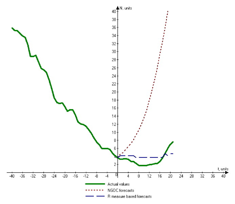
Figure 1: Results of short-dated forecasts comparison

Therefore, the graphic shows that in this case the forecasting method based on R measure was more effective in the producing of the short-dated prediction. There is no information on the NGDC server to carry out other experiments for precision comparison. It goes without saying, that the comparison of forecasting methods with only on file to take into account may be not enough to come to the ultimate conclusions, however, any way the rate of the absolute and relative (we may see that it is about $1\%$) errors, obtained by the investigated method, justifies its right of existence.

Forecasting with preparatory time series transformation. It is known that statistical methods of forecasting are often used with the preparatory transformation of input data. The combination of this approach and the investigated method may improve the precision of prediction. In this subsection experimental estimation of the application of the forecasting method based on the measure $R$ together with the preparatory differentiation of the time series was accomplished. Having such forecast value we can easily add it to the last known elements of time series and obtain the desired prediction Again the subsection includes the study of two items.

One-step ahead forecasts comparison. Here as the target of research time series, consisting of the 15-minute sea level indices, were considered. All datasets used in the experiments of this item, can be found at the British Oceanographic Data Centre (BODC) Internet site in the “UK Tide Gauge Network” section. The web interface of the site allows any registered user to download data file with the history of 15-minute sea level indices for the certain gauge from some location. In this file for each timestamp for the certain period of time the appropriate actual and residual values are given. The latter are calculated from the observed sea level values minus the predicted sea level values. According to the provided by BODC support information predicted tide values are produced at the National Oceanography Centre’s (NOC), using their harmonic tidal analysis. This is based on the TIRA tidal analysis programs following the Doodson method. We considered the data related to the Bubbler tide gauge from Dover and captured in 2005 year, because all values for that period are available and there are no missed or interpolated points there. As in the first item of previous subsection the one-step ahead forecasting was decided here. Furthermore, the scheme of the calculations, using the time series of different length and adaptive mode, was the same, but in this item each estimation series contained 30 experiments. After the accomplishing of all appropriate computations, the precision estimation was made by considering the differences between corresponding forecast and actual values. As we mentioned above the history contains residuals for every element of time series. So, in the purpose of the objectivity for each MAE of NOC software we took into account residuals corresponding only to the values predicted by investigated method. The results of the study of this item are situated in Table 3.

Table 2: Forecasting results 15-minutes sea level indices

Length	500	1000	2000	5000	Adaptive mode
$R$	0.034	0.038	0.0396	0.037	0.037
NOC	0.207	0.2133	0.09883	0.0779	$-$

The first row contains MAE for $R$ measure based method and the appropriate input data. The second row includes MAE for computations produced at the NOC. So it is seen from the table that for the forecast using the described method and the time series of size 5000 the MAE is 0.037 for 30 experiments. And if we consider the given by NOC residuals for each of that 30 predicted by the investigated method values we will obtain 0.0779. There is no information about calculation in appropriate adaptive mode for NOC.

Comparison with the simplest method The simplest test to explore a new forecasting method is a comparison with so-called inertial prediction, where the last actual value is supposed to be the next forecast value. Here we will accomplish this kind of comparison, regarding the FOREX cross-rates daily currencies of US dollar and Great Britain pound to Euro. We used data on the both cross-rates from January 2001, 03 to January 2011, 17. All datasets used in this investigation item were taken from FXHISTORICALDATA.COM. Again we considered the one-step ahead forecasting. Each estimation series contained 10 experiments. After the accomplishing of all appropriate computations, the precision estimation was made by considering the differences between corresponding forecast and actual values. The comparison results are summarized in Table 4 and Table 5.

Table 3: Comparison with the inertial method for USD/EUR cross-rate

Foracasting method	500	1000
$R$	0.00298	0.00582
Inertial	0.0030	0.0059

Table 4: Comparison with the inertial method for GBP/EUR cross-rate

Foracasting method	500	1000
$R$	0.0019	0.00089
Inertial	0.0025	0.0010

Tables have similar structure. The first and the second rows contain the MAE for forecasting method based on $R$ measure and inertial prediction respectively when using the appropriate length of input data. As a whole we may say that the forecasting method based on the universal measure $R$ showed the better than the inertial prediction results.

4 Conclusion

In this article the implementation and experimental estimation of forecasting method, based on the universal measure $R$ were considered. Analysis of the investigation outcomes has shown the quite high precision of the obtained results. Moreover, in comparison of the short-dated forecasts, obtained by the $R$ measure based method and by NGDC software the significant advantage of the former was detected. Good results were also achieved in the combine with preparatory transformation of time series. We found parameters for which the consistent superiority of the considered method in comparison with UK NOC prediction was detected in the one-step ahead forecasting. As a result we may conclude that universal codes are believed to be the effective tool for the forecasting methods construction in practical application.

References

- [1] De Gooijer, J.G. & Hyndman, R.J. (2006) 25 years of time series forecasting. International Journal of Forecasting, 22(3), 443-473
- [2] Fitingof, B.M. (1966). Optimal encoding for unknown and changing statistics of messages. Problems of Information Transmission, 2(2), 3-11.
- [3] FXHISTORICALDATA.COM: URL: http://www.fxhistoricaldata.com/
- [4] Gallager, R.G. (1968). Information Theory and Reliable Communication. John Wiley & Sons, New York.
- [5] Kolmogorov, A.N. (1965). Three approaches to the quantitative definition of information. Problems Inform. Transmission, 1, 3-11.
- [6] Krichevsky, R. (1993). Universal Compression and Retrival, Kluver Academic Publishers,
- [7] Makridakis, S.G., Wheelwright S.C., and Hyndman, R.J. (1998). Forecasting: Methods and Applications, Wiley, (3rd edition).
- [8] Rissanen, J. (1984). Universal coding, information, prediction, and estimation. IEEE Trans. Inform. Theory, 30(4), 629-636.
- [9] Ryabko, B. (1984). Twice-universal coding. Problems of Information Transmission, 20(3), 173-177.
- [10] Ryabko, B. (1988). Prediction of random sequences and universal coding. Problems of Inform. Transmission, 24(2), 87-96.
- [11] Ryabko, B. (2009). Compression-Based Methods for Nonparametric Prediction and Estimation of Some Characteristics of Time Series. IEEE Transactions on Information Theory, 55(9), 4309-4315.
- [12] Ryabko, B. (2010). Applications of Universal Source Coding to Statistical Analysis of Time Series. In: Isaac Woungang et al. (Eds.), Selected Topics in Information and Coding Theory, World Scientific Publishing, pp. 289 - 338. (see also http://arxiv.org/pdf/cs/0701036v2 )
- [13] Ryabko, B. & Astola, J. (2006) Universal Codes as a Basis for Time Series Testing Statistical Methodology, 3, 375-397.
- [14] Ryabko, B. & Monarev, V. (2005). Using Information Theory Approach to Randomness Testing. Journal of Statistical Planning and Inference, 133(1), 95-110
- [15] Space Weather & Solar Events. National Geophysical Data Center: URL: http://www.ngdc.noaa.gov/stp/spaceweather.html
- [16] UK National Tide Gauge Network. British Oceanographic Data Centre: