Temporary mirror symmetry breaking and chiral excursions in open and closed systems

Abstract

The reversible Frank model is capable of amplifying the initial small statistical deviations from the idealized racemic composition. This temporary amplification can be interpreted as a chiral excursion in a dynamic phase space. It is well known that if the system is open to matter and energy exchange, a permanently chiral state can be reached asymptotically, while the final state is necessarily racemic if the system is closed. In this work, we combine phase space analysis, stability analysis and numerical simulations to study the initial chiral excursions and determine how they depend on whether the system is open, semi-open or closed.

I Introduction

The Frank model Frank has been extensively invoked to justify theoretically the emergence of biological homochirality Mason ; PKBCA , and is usually analyzed as a reaction network in open systems (matter and energy are exchanged with the surroundings) composed of an irreversible enantioselective autocatalysis coupled to an irreversible mutual inhibition reaction between the product enantiomers. The model shows how homochirality is achieved as a stationary state when the mutual inhibition product (the heterodimer) is removed from the system and when the concentration of the achiral substrate is held constant. By contrast, for reversible transformations and when the mutual inhibition product remains in the system, the final stable state can only be the racemic one. As a consequence, a thermodynamically controlled spontaneous mirror symmetry breaking (SMSB) cannot be expected to take place. In particular, SMSB is not expected for reversible reactions taking place in systems closed to matter and energy flow.

Nevertheless, as was recently demonstrated CHMR for systems closed to matter flow, the Frank model is a prime candidate for the fundamental reaction network necessary for reproducing the key experimental features reported on absolute asymmetric synthesis in the absence of any chiral polarization Soai . Most importantly, when reversible steps in all the reactions are allowed it is capable of CHMR (i) amplification of the initially tiny statistical enantiomeric excesses from $ee\sim 10^{-8}\%$ to practically 100%, leading to (ii) long duration chiral excursions or chiral pulses away from the racemic state at nearly 100% $ee$, followed by, (iii) the final approach to the stable racemic state for which $ee=0$, i.e., mirror symmetry is recovered permanently. To understand this temporary asymmetric amplification is important because the racemization time scale can be much longer than that for the complete conversion of the achiral substrate into enantiomers.

Long duration chiral excursions have also been reported recently in closed chiral polymerization models with reversible reactions BH where constraints implied by microreversibility have been taken into account. These results are important because they suggest that temporary spontaneous mirror symmetry breaking in experimental chiral polymerization can take place, and with observable and large chiral excesses without the need to introduce chiral initiators Lahav or large initial chiral excesses Hitz .

The purpose of this Letter is to elucidate the nature of these chiral excursions by combining the information provided by phase plane portraits, numerical simulation and linear stability analysis. We consider the Frank model, this being the most amenable to such types of analysis and because it is the “common denominator” of numerous more elaborate theoretical models of SMSB PKBCA .

The reaction scheme consists of a straight non-catalyzed reaction Eq. (1), an enantioselective autocatalysis Eq. (2), where A is a prechiral starting product, and L and D are the two enantiomers of the chiral product. We also assume reversible heterodimerization step in Eq. (3), where LD is the achiral heterodimer. The $k_{i}$ denote the reaction rate constants. In the following, we give the reaction steps in detail.

Production of chiral compound:

$$\textrm{A}\stackrel{{\scriptstyle k_{1}}}{{\rightleftharpoons\atop{k_{-1}}}}\textrm{L},\qquad\textrm{A}\stackrel{{\scriptstyle k_{1}}}{{\rightleftharpoons\atop{k_{-1}}}}\textrm{D}.$$ (1)

Autocatalytic amplification:

$$\textrm{L}+\textrm{A}\stackrel{{\scriptstyle k_{2}}}{{\rightleftharpoons\atop{k_{-2}}}}\textrm{L}+\textrm{L},\qquad\textrm{D}+\textrm{A}\stackrel{{\scriptstyle k_{2}}}{{\rightleftharpoons\atop{k_{-2}}}}\textrm{D}+\textrm{D}.$$ (2)

Hetero-dimerization:

$$\textrm{L}+\textrm{D}\stackrel{{\scriptstyle k_{5}}}{{\rightleftharpoons\atop{k_{-5}}}}\textrm{LD}.$$ (3)

We assume the feasibility of the reverse reaction for all the steps. Focusing our attention on chiral excursions, we make a careful distinction between open, semi-open or fully closed systems. These system constraints are crucial for determining both the intermediate and the asymptotic final states of the chemical system.

II Open system

II.1 Rate equations

We first consider the original Frank scenario Frank . There, steady and stable chiral states can be achieved, since the system is permanently held out of equilibrium. See RH for more details. An important question is, can the system support chiral excursions? That is, pass through temporary chiral states before ending up in the final racemic state? In the original Frank model there is an incoming flow of achiral compound A and elimination of the heterodimer LD from the system. A convenient way to account for the inflow of achiral matter is to assume that the concentration of the prechiral component $[A]$ is constant, and then we need not write the corresponding kinetic equation for it. For the outflow the heterodimer leaves the system at a rate $\bar{\gamma}$. We assume that the heterodimer formation step is irreversible, and set $k_{-5}=0$. Note, the elimination of LD from the system can actually be neglected as long as the hetero-dimerization step is irreversible PKBCA . We retain this outflow however since it is needed to obtain stationary asymptotic values of all three concentrations $[L],[D]$ and $[LD]$; see the fixed points below. So with $[A]=const$ and replacing Eq. (3 ) by

$$\textrm{L}+\textrm{D} \stackrel{{\scriptstyle k_{5}}}{{\rightarrow}} \textrm{LD},$$ (4)

LD $$\stackrel{{\scriptstyle\bar{\gamma}}}{{\rightarrow}} \emptyset,$$ (5)

we obtain the rate equations

$$\frac{d}{dt}[L] = k_{1}[A]+(k_{2}[A]-k_{-1})[L]-k_{-2}[L]^{2}-k_{5}[L][D],$$ (6)

$$\frac{d}{dt}[D] = k_{1}[A]+(k_{2}[A]-k_{-1})[D]-k_{-2}[D]^{2}-k_{5}[D][L],$$ (7)

$$\frac{d}{dt}[LD] = k_{5}[L][D]-\bar{\gamma}[LD].$$ (8)

The key variable throughout is the chiral polarization

$$\eta=\frac{[L]-[D]}{[L]+[D]},$$ (9)

also called enantiomeric excess $ee$, which obeys $-1\leq\eta\leq 1$ and which represents the order parameter for mirror symmetry breaking.

In order to simplify the analysis, we define a dimensionless time parameter $\tau=(k_{2}[A]-k_{-1})t$ and dimensionless concentrations that scale as $[\tilde{L}]=k_{5}(k_{2}[A]-k_{-1})^{-1}[L]$, $[\tilde{D}]=k_{5}(k_{2}[A]-k_{-1})^{-1}[D]$, $[\widetilde{LD}]=k_{5}(k_{2}[A]-k_{-1})^{-1}[LD]$. It is convenient to define the sums and differences of concentrations: $\chi=[\tilde{L}]+[\tilde{D}]$, $y=[\tilde{L}]-[\tilde{D}]$, and for the heterodimer put $P=[\widetilde{LD}]$. The chiral polarization $\eta=y/\chi$ remains unchanged.

In terms of the new variables, Eqs. (6-8) read

$$\frac{d\chi}{d\tau} = 2u+\chi-\frac{1}{2}(g+1)\chi^{2}-\frac{1}{2}(g-1)\chi^{2}\eta^{2},$$ (10)

$$\frac{d\eta}{d\tau} = \eta(1-g\chi)-\frac{\eta}{\chi}\left(\frac{d\chi}{d\tau}\right),$$ (11)

$$\frac{dP}{d\tau} = \frac{1}{4}\chi^{2}(1-\eta^{2})-\gamma P.$$ (12)

The dimensionless parameters appearing here are:

$$u=\frac{k_{1}k_{5}[A]}{(k_{2}[A]-k_{-1})^{2}},\,\,g=\frac{k_{-2}}{k_{5}},\,\,\gamma=\frac{\bar{\gamma}}{(k_{2}[A]-k_{-1})}.$$ (13)

The system is described by three equations Eqs. (10-12). Since $P$ does not enter into the equations for $\chi$ and $\eta$, the equations decouple and the dynamical system to study is effectively two-dimensional and so the appearance of SMSB cannot depend on whether the heterodimer is removed from the system when $k_{-5}=0$, although the fixed points will (see Sec II.3).

II.2 Phase plane and linear stability analysis

In the phase space of the dynamical system defined by Eqs. (10,11) there are curves with a special significance. These are the nullclines defined by

$$\frac{d\chi}{d\tau} = 0,$$ (14)

$$\frac{d\eta}{d\tau} = 0.$$ (15)

The intersections of these curves give the possible steady states (or fixed points) of the system. The condition $d\chi/d\tau=0$ leads to two curves

$$\chi_{\pm}^{(1)}=\frac{1\pm\sqrt{1+4u(g(1+\eta^{2})+1-\eta^{2})}}{g(1+\eta^{2})+1-\eta^{2}},$$ (16)

while $d\eta/d\tau=0$ implies the three curves

$$\eta=0,\qquad\chi_{\pm}^{(2)}=\pm\sqrt{\frac{4u}{1-g+(g-1)\eta^{2}}}.$$ (17)

For $u>0$ the solutions denoted $\chi_{-}$ correspond to negative total enantiomer concentrations so we discard them. The physically acceptable nullclines are plotted in Fig. 1. Which of the two different intersection configurations is obtained depends only on the single parameter $g$. We emphasize that despite the similar appearance, the nullcline graphs should not be confused with the classic bifurcation diagrams that have been discussed often in the past MKG ; Kondepudi ; Avetisov .

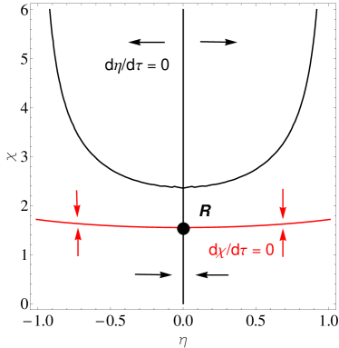
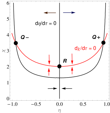
Figure 1: Nullclines for the open system (10,11). These curves correspond to $u=0.3$ implying $g_{crit}=0.59$. The $d\eta/d\tau=0$ and $d\chi/d\tau=0$ nullclines are plotted in black and red, respectively. The black (red) arrows indicate the regions of phase space where $\eta$ ($\chi$) increases or decreases. Left: $g=0.79>g_{crit}$. The nullclines intersect in only the one point $R$ representing the asymptotic stable racemic state. Right: $g=0.29<g_{crit}$. In this case there are three intersections, $Q_{\pm}$ and $R$ representing the $Z_{2}$ equivalent stable chiral states and the unstable racemic state, respectively. From Eq. (22) the enantiomeric excess at $Q_{\pm}$ is $\eta=\pm 0.93$.

II.3 Fixed Points and Stability

The system has several steady states: besides an unphysical state that we disregard, there is a $Z_{2}$ pair of chiral solutions $Q_{\pm}$, and a racemic state $R$:

$$R = \Big{(}P=\frac{2(g+1)u+\sqrt{4(g+1)u+1}+1}{2(g+1)^{2}\gamma},\chi=\frac{1+\sqrt{4(g+1)u+1}}{g+1},y=0\Big{)},$$ (18)

$$Q_{\pm} = \Big{(}P=\frac{u}{\gamma-g\gamma},\chi=\frac{1}{g},y=\pm\frac{\sqrt{((g-1)/g^{2})+4u}}{\sqrt{g-1}}\Big{)}.$$ (19)

The associated eigenvalues are given by RH :

$$\lambda_{1,2,3}(R) = \Big{(}-\sqrt{4(g+1)u+1},\frac{1-g\sqrt{4(g+1)u+1}}{g+1},-\gamma\Big{)},$$ (20)

$$\lambda_{1,2,3}(Q_{\pm}) = \Big{(}\frac{-\sqrt{16g^{3}u+4g^{2}-4g+1}-1}{2g},\frac{\sqrt{16g^{3}u+4g^{2}-4g+1}-1}{2g},-\gamma\Big{)}.$$ (21)

Note that $\lambda_{1}(R)<0$ and $\lambda_{1}(Q)<0$ are always negative whereas $\lambda_{2}(R)>0$ and $\lambda_{2}(Q)<0$ for $g<g_{crit}$, otherwise $\lambda_{2}(R)<0$ and $\lambda_{2}(Q)>0$ for $g>g_{crit}$, where $g_{crit}=(\sqrt{1+16u}-1)/8u$ is the critical value for this parameter. Note that $g_{crit}(u)\leq 1$ for all $u\geq 0$. For small $u$ we can write $g_{crit}=1-4u$; while for large $u$, $g_{crit}\rightarrow 1/2u^{1/2}$. Thus the direct chiral monomer production step ($\propto k_{1}$ in (1)) tends to racemize the system leading to final $\eta$ values strictly less than unity:

$$\eta=\pm\sqrt{1-\frac{4ug^{2}}{1-g}}\,\,,$$ (22)

which holds when $g<g_{crit}$. The chiral monomer production step thus reduces the range of $g$ for which stable mirror symmetry breaking can occur, and the chiral solutions are no longer $100\%$ chiral.

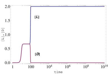
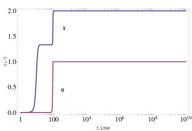
Figure 2: Chiral symmetry breaking in the open system (6-8). Temporal behavior (logarithmic scale) of the individual enantiomer concentrations $[L]$ and $[D]$ (left), and the chiral polarization $\eta$ and total enantiomer concentration $\chi$ (right). Initial concentrations: $[L]_{0}=(1\times 10^{-6}+1\times 10^{-15})M$, $[D]_{0}=1\times 10^{-6}M$ ($\eta_{0}=5\times 10^{-8}\%$) and $[A]=1M$. Rate constants: $k_{1}=10^{-4}s^{-1}$, $k_{-1}=10^{-6}s^{-1}$, $k_{2}=1s^{-1}M^{-1}$, $k_{-2}=0.5s^{-1}M^{-1}$ and $k_{5}=1s^{-1}M^{-1}$. These values correspond to $g=0.5$ and $u=10^{-4}$. In figures of simulations, we always display original variables $[L],[D],[LD]$, etc. as function of time $t$.

Figure 2 shows the temporal evolution of the L and D chiral monomers starting from an extremely dilute total enantiomer concentration and the very small statistical chiral deviations from the ideal racemic composition. The right hand side of this figure shows the evolution in terms of the quantities $\chi$ and $\eta$. Note the mirror symmetry breaking signalled by $\eta$. Are there chiral excursions found in the open system model? A chiral excursion holds when the enantiomeric excess $\eta$ departs from a small initial value, evolves to some maximum absolute value and then decays to the final value of zero. To ensure a final racemic state we must set $g>g_{crit}$ but then we find no numerical evidence for such temporary chiral excursions. This can be understood qualitatively from inspection of left hand side of Fig. 1. The initial conditions (dilute chiral monomer concentration and statistical chiral fluctuation) corresponds to a initial point located at tiny values of $\chi$ and close to the vertical nullcline, well below the point labeled as $R$. The system is attracted to the black curve and moves up the curve to $R$. In this situation, it is impossible for the chiral excess to increase, not even temporarily. Notice the time scales for $\chi$ and $\eta$ are of the same order. On the other hand, if $g<g_{crit}$, then we have the situation depicted on the right hand side of the figure. Here the same initial point moves towards the vertical nullcline and up towards $R$, but once past the locally horizontal black curve, is attracted to one of the two chiral fixed points where it stays forever, provided the system is maintained out of equilibrium. The chiral symmetry is permanently broken, and there is no excursion such as we have defined it.

III Semi-open system

III.1 Rate equations

To elucidate the temporal evolution of $\chi$ and $\eta$ for a more general setting, we do not remove the heterodimer from the system now allow the back reaction to chiral monomers, and we keep [A] constant. There is an implicit inflow as a consequence of constant $[A]$, but no outflow, so we denote this case ”semi-open”. While there is no mass balance the system can still exhibit temporary SMSB.

The corresponding rate equations are

$$\frac{d}{dt}[L] = k_{1}[A]+(k_{2}[A]-k_{-1})[L]-k_{-2}[L]^{2}-k_{5}[L][D]+k_{-5}[LD],$$ (23)

$$\frac{d}{dt}[D] = k_{1}[A]+(k_{2}[A]-k_{-1})[D]-k_{-2}[D]^{2}-k_{5}[D][L]+k_{-5}[LD],$$ (24)

$$\frac{d}{dt}[LD] = k_{5}[L][D]-k_{-5}[LD].$$ (25)

After performing the same rescaling as in the open case, we arrive at

$$\frac{d\chi}{d\tau} = 2u+\chi-\frac{1}{2}(g+1)\chi^{2}-\frac{1}{2}(g-1)\chi^{2}\eta^{2}+2rP,$$ (26)

$$\frac{d\eta}{d\tau} = \eta(1-g\chi)-\frac{\eta}{\chi}\left(\frac{d\chi}{d\tau}\right),$$ (27)

$$\frac{dP}{d\tau} = \frac{1}{4}\chi^{2}(1-\eta^{2})-rP.$$ (28)

The dimensionless parameters appearing here are:

$$u=\frac{k_{1}k_{5}[A]}{(k_{2}[A]-k_{-1})^{2}},\,\,g=\frac{k_{-2}}{k_{5}},\,\,r=\frac{k_{-5}}{(k_{2}[A]-k_{-1})}.$$ (29)

The system is described by three equations Eqs. (26-28) which do not decouple.

III.2 Phase plane and linear stability analysis

In order to obtain an approximate two-dimensional phase plane representation of the system, we will invoke the dynamic steady state approximation for the heterodimer. Such approximations are usually justified when there exists a clear separation of time scales in the problem, thus allowing one to identify rapidly and slowly changing concentrations Scott . Here however, no such time scales are evident, all concentration variables evolve on a similar time scale. Nevertheless, we will see a posteriori that this approximation can be good over a wide range of time scales. We therefore assume that the heterodimer is in a dynamic steady state $P_{stat}$ relative to the chiral monomer concentrations and chiral polarization:

$$P_{stat}\approx\frac{\chi^{2}}{4r}(1-\eta^{2}).$$ (30)

Substituting this $P_{stat}$ into Eqs. (26,27) leads to the differential equations

$$\frac{d\chi}{d\tau} = 2u+\chi-\frac{g}{2}\chi^{2}(1+\eta^{2}),$$ (31)

$$\frac{d\eta}{d\tau} = \eta\Big{(}-g\chi-\frac{2u}{\chi}+\frac{g}{2}\chi(1+\eta^{2})\Big{)}.$$ (32)

As above, we study the phase space of the two-dimensional system by means of the nullclines. These are plotted in Fig. 3. The condition $d\chi/d\tau=0$ implies two curves

$$\chi_{\pm}=\frac{1\pm\sqrt{1+4gu(1+\eta^{2})}}{g(1+\eta^{2})},$$ (33)

whereas the condition $d\eta/d\tau=0$ implies the three curves

$$\eta=0,\qquad\eta_{\pm}=\pm\sqrt{1+\frac{4u}{g\chi^{2}}}.$$ (34)

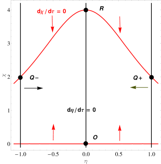
Figure 3: Nullclines for the semi-open case (31,32) in the steady state approximation for $P$. The nullclines (33,34) are plotted in red and black, respectively. Red and black arrows indicate the phase-space regions of increasing or decreasing $\chi$ and $\eta$. The four stationary solutions $O,R,Q_{\pm}$ are indicated by the black dots. These curves are illustrated for $u=0$ and $g=0.5$.

III.3 Fixed Points and Stability

We solve Eqs. (26-28) looking for steady states. To keep the algebra manageable, we also set $u=0$ as in RH . There are four solutions, namely, the empty $O$ solution, the racemic $R$ or the two mirror-symmetric chiral $Q_{\pm}$ solutions:

$$O = (P=0,\chi=0,y=0),$$ (35)

$$R = \left(P=\frac{1}{g^{2}r},\chi=\frac{2}{g},y=0\right),$$ (36)

$$Q_{\pm} = \left(P=0,\chi=\frac{1}{g},y=\pm\frac{1}{g}\right).$$ (37)

Note that the final heterodimer concentration $P$ is zero in the chiral states $Q_{\pm}$. Note that the steady state approximation Eq. (30) implies the same result since $|\eta|=1$. In order to study the linear stability of the four possible homogeneous solutions $O,R$ and $Q_{\pm}$, we calculate the eigenvalues of the $3\times 3$ Jacobian array $M_{open}$ derived in RH after deleting the 3rd and 4th rows and columns. The eigenvalues corresponding to these solutions are given by

$$\lambda_{1,2,3}(O) = (1,1,-r),$$ (38)

$$\lambda_{1,2,3}(R) = \Big{(}-1,\,-\frac{2+g(1+r)+\sqrt{4+g^{2}(-1+r)^{2}+4g(1+r)}}{2g},$$ (39)

$$\frac{-2-g(1+r)+\sqrt{4+g^{2}(-1+r)^{2}+4g(1+r)}}{2g}\Big{)}.$$

$$\lambda_{1,2,3}(Q_{\pm}) = \Big{(}-1,\,-\frac{1+g(-1+r)+\sqrt{1+2g(-1+r)+g^{2}(1+r)^{2}}}{2g},$$ (40)

$$\frac{-1+g(1-r)+\sqrt{(1+g(-1+r))^{2}+4g^{2}r}}{2g}\Big{)}.$$

As $\lambda_{1,2}(O)>0$, the empty state is always unstable. An inequality analysis shows that both $\lambda_{2}(R)<0$ and $\lambda_{3}(R)<0$ for all $r>0$ and $g>0$. Since $\lambda_{1}(R)=-1$ this demonstrates that the racemic state $R$ is always stable. As an independent check, we also verify that $\lambda_{3}(Q)>0$ is positive for all $r>0$ and $g>0$, so the chiral solutions $Q_{\pm}$ are always unstable. The final outcome will always the racemic state. There is no stable mirror symmetry broken solution when the heterodimer dissociates back into the chiral monomers. Nevertheless, the system can have temporary chiral excursions.

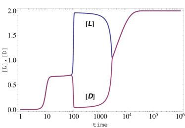
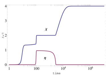
Figure 4: Temporary chiral symmetry breaking and chiral excursions in the semi-open system (23-25). Temporal behavior (logarithmic scale) of the individual enantiomer concentrations $[L]$ and $[D]$ (left) and the chiral polarization $\eta$ and total enantiomer concentration $\chi$ (right). Initial concentrations: $[L]_{0}=(1\times 10^{-7}+1\times 10^{-15})M$, $[D]_{0}=1\times 10^{-7}M$ ($\eta_{0}=5\times 10^{-8}\%$) and $[A]=1M$. Rate constants: $k_{1}=10^{-4}s^{-1}$, $k_{-1}=10^{-6}s^{-1}$, $k_{2}=1s^{-1}M^{-1}$, $k_{-2}=0.5s^{-1}M^{-1}$, $k_{5}=1s^{-1}M^{-1}$ and $k_{-5}=10^{-3}s^{-1}$. These rate constants imply $g=0.5$ and $u=10^{-4}$.

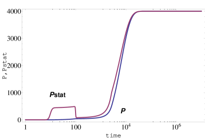
Figure 5: Semi-open system: Comparison of direct numerical solution $P=[\widetilde{LD}]$ and the steady state approximation $P_{stat}$ in Eq. (30) for the heterodimer concentration (after transforming from $[L],[D],[LD]$ to $\chi,\eta,P$).

In Fig. 4 we plot the temporal evolution of the $L$ and $D$ chiral monomers starting from an extremely dilute total enantiomer concentration and the very small statistical chiral deviations from the ideal racemic composition. The right hand side of this figure shows the evolution in terms of the quantities $\chi$ and $\eta$. Note the chiral excursion in $\eta$ for the time interval between $t\simeq 100s$ and $t\simeq 1000s$. Finally, we compare the heterodimer concentration from direct numerical simulation with the steady state approximation in Fig. 5. To do so we simulate the original concentration variables in Eqs.(23-25) and then transform results in terms of $\chi$, $\eta$ and $P$. While $P_{stat}$ appears to overestimate $P=[\widetilde{LD}]$, it provides a reasonably good approximation to the actual heterodimer concentration $P$ right after chiral symmetry is broken, at about $t\simeq 100s$ and coincides perfectly after chiral symmetry is recovered, and when $\chi$ reaches its asymptotic value, after approximately $t\simeq 10^{4}s$.

IV Closed system

IV.1 Rate equations

The rate equations directly follow from (1-3):

$$\frac{d}{dt}[L] = k_{1}[A]+(k_{2}[A]-k_{-1})[L]-k_{-2}[L]^{2}-k_{5}[L][D]+k_{-5}[LD],$$ (41)

$$\frac{d}{dt}[D] = k_{1}[A]+(k_{2}[A]-k_{-1})[D]-k_{-2}[D]^{2}-k_{5}[D][L]+k_{-5}[LD],$$ (42)

$$\frac{d}{dt}[A] = -2k_{1}[A]-(k_{2}[A]-k_{-1})([L]+[D])+k_{-2}([L]^{2}+[D]^{2}),$$ (43)

$$\frac{d}{dt}[LD] = k_{5}[L][D]-k_{-5}[LD].$$ (44)

There is no flow of material into or out of the system. Since $[A]$ is not constant in this situation, we cannot use it to rescale the time or the concentrations. Instead, we take $\tau=k_{1}t$ for the time parameter and $[\tilde{L}]=(k_{5}/k_{1})[L]$, etc. for the dimensionless concentrations. This allows us to express the rate equations in the following dimensionless form:

$$\frac{d}{d\tau}[\tilde{L}] = [\tilde{A}]-u[\tilde{L}]+h[\tilde{A}][\tilde{L}]-g[\tilde{L}]^{2}-[\tilde{L}][\tilde{D}]+\rho[\widetilde{LD}],$$ (45)

$$\frac{d}{d\tau}[\tilde{D}] = [\tilde{A}]-u[\tilde{D}]+h[\tilde{A}][\tilde{D}]-g[\tilde{D}]^{2}-[\tilde{D}][\tilde{L}]+\rho[\widetilde{LD}],$$ (46)

$$\frac{d}{d\tau}[\widetilde{LD}] = [\tilde{L}][\tilde{D}]-\rho[\widetilde{LD}].$$ (47)

These are subject to the constraint $[\tilde{A}]=[\tilde{C}]-([\tilde{L}]+[\tilde{D}])-2[\widetilde{LD}]$, where $[\tilde{C}]=(k_{5}/k_{1})[C]$ and $[C]$ is the total initial concentration, being constant in time. The four parameters appearing here are

$$u=\frac{k_{-1}}{k_{1}},\,g=\frac{k_{-2}}{k_{5}},\,h=\frac{k_{2}}{k_{5}},\,\rho=\frac{k_{-5}}{k_{1}}.$$ (48)

Changing variables as before to $\chi,\eta,P$, we arrive at

$$\frac{d\chi}{d\tau} = 2[\tilde{A}]+(h[\tilde{A}]-u)\chi-\frac{1}{2}(g+1)\chi^{2}-\frac{1}{2}(g-1)\chi^{2}\eta^{2}+2\rho P,$$ (49)

$$\frac{d\eta}{d\tau} = \eta(h[\tilde{A}]-g\chi-u)-\frac{\eta}{\chi}\left(\frac{d\chi}{d\tau}\right),$$ (50)

$$\frac{dP}{d\tau} = \frac{1}{4}\chi^{2}(1-\eta^{2})-\rho P.$$ (51)

In these variables, the constant mass constraint reads $[\tilde{A}]=[\tilde{C}]-\chi-2P$.

IV.2 Phase plane and linear stability analysis

As in the semi-open case, to obtain an approximate two-dimensional phase plane portrait, we assume that the heterodimer is in an approximate steady state $P_{stat}$ and solve Eq. (51) for

$$P_{stat}\approx\frac{\chi^{2}}{4\rho}(1-\eta^{2}).$$ (52)

Substituting this back into Eqs. (49,50), we obtain

$$\frac{d\chi}{d\tau} = (2+h\chi)[\tilde{A}]-u\chi-\frac{g}{2}\chi^{2}(1+\eta^{2}),$$ (53)

$$\frac{d\eta}{d\tau} = \eta\Big{(}-g\chi-\frac{2[\tilde{A}]}{\chi}+\frac{g}{2}\chi(1+\eta^{2})\Big{)},$$ (54)

where

$$[\tilde{A}] = [\tilde{C}]-\chi-\frac{\chi^{2}}{2\rho}(1-\eta^{2}).$$ (55)

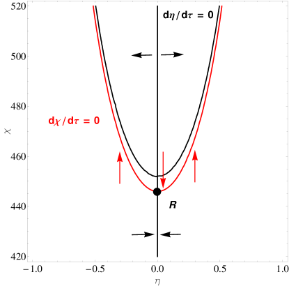
Figure 6: Nullclines for the closed system (53,54) in the steady state approximation for $P$. The $\eta$ and $\chi$ nullclines are plotted as the black and red curve, respectively. These nullclines intersect at the one point (indicated with a dot) which corresponds to the stable racemic solution $R$ with $\eta=0$ and $\chi>0$. The flow directions are indicated with arrows. This diagram corresponds to the parameter values $g=0.05$, $u=0.01$, $h=0.1$ and $\rho=1.0$ and $[\tilde{C}]=10^{5}$.

The nullcline condition $d\chi/d\tau=0$ leads to an unwieldy cubic equation in $\chi$. More importantly, the nullcline is an even function of $\eta$, reflecting the underlying $Z_{2}$ mirror symmetry. The other condition $d\eta/d\tau=0$ is straightforward to solve analytically and leads – after discarding the unphysical solution corresponding to negative total enantiomer concentrations – to two curves

$$\eta=0,\qquad\chi=\frac{-1+\sqrt{1+2{[\tilde{C}]}(g(1+\eta^{2})/2+(1-\eta^{2})/\rho-g)}}{g(1+\eta^{2})/2+(1-\eta^{2})/\rho-g}.$$ (56)

The curve $\chi(\eta)$ is an even function of $\eta$ and $\chi(\eta)\rightarrow\infty$ for $\eta^{2}\rightarrow 1$ with a minimum at $\eta=0$. Thus the nullcline has the form of a narrow fork as depicted in Fig. 6.

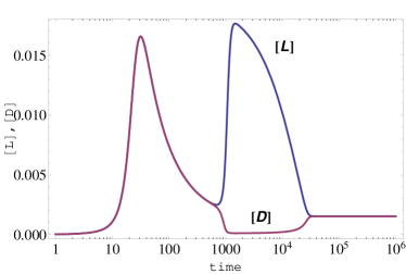
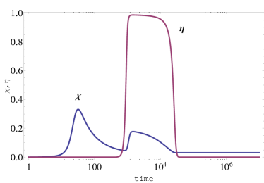
Figure 7: Temporary chiral symmetry breaking and chiral excursions in the closed system (41-42). Temporal behavior (logarithmic scale) of the individual enantiomer concentrations $[L]$ and $[D]$ (left) and the chiral polarization $\eta$ and total enantiomer concentration $\chi$ (right). Initial concentrations: $[L]_{0}=(1\times 10^{-7}+1\times 10^{-15})M$, $[D]_{0}=1\times 10^{-7}M$ ($\eta_{0}=5\times 10^{-8}\%$) and $[A]_{0}=1M$. Rate constants: $k_{1}=10^{-4}s^{-1}$, $k_{-1}=10^{-6}s^{-1}$, $k_{2}=1s^{-1}M^{-1}$, $k_{-2}=0.5s^{-1}M^{-1}$, $k_{5}=10s^{-1}M^{-1}$ and $k_{-5}=10^{-4}s^{-1}$.

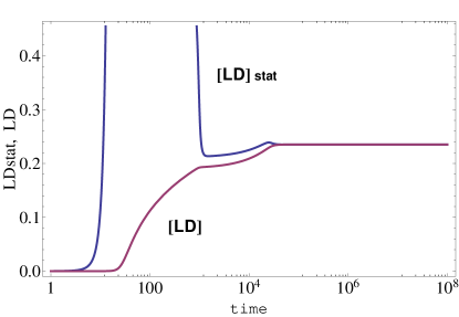
Figure 8: Comparison of direct numerical solution $[LD]$ and the steady state approximation $[LD]_{stat}=(k_{5}/k_{-5})[L][D]$ for the heterodimer concentration. The steady state approximation peaks to a maximum value of about 25 in this example.

IV.3 Fixed Points and Stability

A linear stability analysis for the closed Frank model is given in RH . That analysis was carried out in terms of $\chi,y$ and $P$ and does not assume the stationary approximation for the heterodimer. It turns out, even in a model as simple as this one, that keeping $\rho>0$ is analytically untractable, so we consider $\rho=0$ in what follows. Then the asymptotic stationary racemic $R$ and chiral solutions $Q_{\pm}$ are given by

$$R = \Big{(}P=\frac{[\tilde{C}]}{2},\chi=0,y=0\Big{)},$$ (57)

$$Q_{\pm} = \Big{(}P=\frac{[\tilde{C}]g+u}{2g},\chi=-\frac{u}{g},y=\pm\frac{u}{g}\Big{)}.$$ (58)

The chiral solutions $Q_{\pm}$ are unphysical for all $u>0$ since they imply negative total enantiomer concentrations $\chi<0$. Thus, the only physically acceptable solution is the racemic one $R$, and this is (at least marginally) stable, the corresponding eigenvalue was calculated to be RH

$$\lambda_{1,2,3}(R)=(0,-2-u,-u).$$ (59)

In the limit $\rho=0$, the substrate is consumed and all the matter ends up finally as pure heterodimer. Finally, note that $\lim_{u\rightarrow 0}Q_{\pm}=R$: the unphysical chiral solutions merge to the racemic one when $k_{-1}=0$. For reversible heterodimer, the matter in the racemic state $\eta=0$ is distributed between the chiral monomers and the heterodimer: $P=([\tilde{C}]-\chi)/2$ and $\chi>0$ in keeping with the law of mass action. The single intersection $R$ displayed in Fig. 6 indicates that the racemic state is the only possible solution, in qualitative agreement with the stability analysis.

Example of a chiral excursion in a closed system is provided in Fig. 7. Once again, as for the semi-open situation, the scheme is capable of amplifying a tiny initial chiral excess to practically $100\%$, followed by final approach to the racemic state. The steady state approximation for the heterodimer is rather poor during the early stages (Fig. 8), but similar to semi-open case, converges to the true heterodimer concentration after symmetry breaking and restoration.

V Discussion

In this Letter, we investigated transient mirror symmetry breaking in chiral systems, in particular in the Frank model in settings of open, semi-open, and closed environments. Temporary chiral excursions are observed for closed and semi-open systems and explained through phase space analysis, stability analysis and numerical simulations. Such chiral excursions may be experimentally observed and could be mistaken for a transition to a chiral state. They are in fact a long sought goal for the experimental chemist who could actually fail to see them if not aware of their transitory nature. In open systems by contrast, the racemic state is approached monotonically. Therefore, it is important to understand the processes and constraints responsible for these outcomes. This Letter has focused on the effects that the in- and outflow of matter has on these phenomena. The open nature of the Frank model can be arranged experimentally with an incoming flow of achiral precursor A and an outflow of the product heterodimer LD, to conserve mass balance. Mathematically, we can model the inflow by assuming a constant concentration of $[A]$ and the outflow by a term representing the rate at which LD leaves the system. In our open model we assumed no dissociation of LD back into chiral monomers. From the point of view of achieving permanent SMSB, there is then actually no need to remove LD from the system, but we retain this outflow since it is needed to ensure stationary fixed points for all the chemical concentrations. For the semi-open case, LD is not removed and we allow for its dissociation into chiral monomers. There is no mass balance but temporary symmetry breaking can arise. Finally, in the closed system there is neither inflow nor outflow, total mass is conserved and temporary symmetry breaking can occur.

A recent kinetic analysis of the Frank model in closed systems applied to the Soai reaction Soai indicates that in actual chemical scenarios, reaction networks that exhibit SMSB are extremely sensitive to chiral inductions due to the presence of inherent tiny initial enantiomeric excesses CHMR . This amplification feature is also operative in much more involved reaction networks such as chiral polymerization BH . When the system is subject to a very small perturbation about an extremely dilute racemic state, the initial chiral fluctuation does not immediately decay, but becomes amplified and drives the system along a long-lived chiral excursion in phase space before final and inevitable approach to the stable racemic solution. Mauksch and Tsogoeva have also previously indicated that chirality could appear as the result of a temporary asymmetric amplification MS1 ; MS2 .

Excursions in phase space as studied in this work are superficially reminiscent of excitable systems as studied in dynamical systems Scott ; Meron ; Goldbeter . But there are important differences. First of all, the excursions reported in chiral systems are not easily visualized in the chiral monomer concentrations themselves, but are strikingly manifested by the chiral polarization or enantiomeric excess. Secondly, the total enantiomer and heterodimer concentrations do increase with time, so that the complete phase-space trajectory does not follow a closed path: there is no return to the initial state. The chiral excursion is a one way trip, not a round trip as in an excitable system. Third, whereas excursions are traditionally studied for open excitable systems Scott ; Meron ; Goldbeter , chiral excursions are observed here only for closed or at most semi-open systems, but not for open systems.

The original impetus for considering phase-space descriptions of the Frank model comes not only from the chiral excursions reported in CHMR and BH but also by the recent report of damped chiral oscillations detected numerically in a model of chiral polymerization in closed systems BH . Absolute asymmetric synthesis is achieved in the latter scheme, accompanied by long duration chiral excursions in the enantiomeric excesses for all the homopolymer chains formed, analogous to the much simpler Frank model. But unlike the latter, strong enantiomeric inhibition converts these excursions into long period damped chiral oscillations in the enantiomeric excesses associated with the longest homochiral polymer chains formed. Moreover, short period sustained chiral oscillations have been observed numerically in a recycled Frank model open to energy flow, for large values of the inhibition Plasson . This oscillatory behavior poses an additional problem for the origin of biological homochirality, since any memory of the sign of the initial fluctuation is further erased by subsequent oscillations thus adding a further element of uncertainty to the overall problem. Chemical oscillations have been traditionally studied in conjunction with excitability. Although the latter concept is not directly applicable to models exhibiting SMSB, it remains to be seen if the techniques used to study oscillations can be applied profitably to reaction schemes that lead to chiral oscillations.

References

- (1) F.C. Frank, Biochim. et Biophys. Acta 11 (1953) 459.
- (2) S.F. Mason Chemical Evolution, Oxford Univ. Press, Oxford, 1991.
- (3) R. Plasson, D.K. Kondepudi, H.Bersini, A. Commeyras and K. Asakura, Chirality 19 (2007) 589.
- (4) J. Crusats, D. Hochberg, A. Moyano and J.M. Ribó, ChemPhysChem 10 (2009) 2123.
- (5) K. Soai, K.T. Shibata, H. Morioka and K. Choji, Nature 378 (1995) 767.
- (6) C. Blanco and D. Hochberg, Phys. Chem. Chem. Phys. 13 (2011) 839.
- (7) I. Weissbuch, R.A. Illos, G. Bolbach and M. Lahav, Acc. Chem. Res. 42 (2009) 1128.
- (8) T. Hitz and P. L. Luisi, Helv. Chim. Acta 86 (2003) 1423.
- (9) J.M. Ribó and D. Hochberg, Phys. Lett. A 373 (2008) 111.
- (10) L.L. Morozov, V.V. Kuzmin and V.I. Goldanskii, Orig. Life 13 (1983) 119.
- (11) D.K. Kondepudi and G.W. Nelson, Physica A 125 (1984) 465.
- (12) V.A. Avetisov, V.V. Kuzmin and S.A. Anikin, Chem. Phys. 112 (1987) 179.
- (13) S.K. Scott, Oscillations, Waves, and Chaos in Chemical Kinetics, Oxford Univ. Press, Oxford, 1994.
- (14) M. Mauksch, S.B. Tsogoeva, S.-W. Wei and I.M. Martinova, Chirality 19 (2007) 816.
- (15) M. Mauksch and S.B. Tsogoeva, ChemPhysChem 9 (2008) 2359.
- (16) E. Meron, Phys. Rep. 218 (1992) 1.
- (17) Albert Goldbeter, Biochemical Oscillations and Cellular Rhythms, Cambridge Univ. Press, Cambridge, 1996.
- (18) R. Plasson, H. Bersini and A. Commeyras, Proc. Natl. Acad. Sci. USA 101 (2004) 16733.