Transcription factor search for a DNA promoter in a three-states model

Abstract

To ensure fast gene activation, Transcription Factors (TF) use a mechanism known as facilitated diffusion to find their DNA promoter site. Here we analyze such a process where a TF alternates between 3D and 1D diffusion. In the latter (TF bound to the DNA), the TF further switches between a fast translocation state dominated by interaction with the DNA backbone, and a slow examination state where interaction with DNA base pairs is predominant. We derive a new formula for the mean search time, and show that it is faster and less sensitive to the binding energy fluctuations compared to the case of a single sliding state. We find that for an optimal search, the time spent bound to the DNA is larger compared to the 3D time in the nucleus, in agreement with recent experimental data. Our results further suggest that modifying switching via phosphorylation or methylation of the TF or the DNA can efficiently regulate transcription.

Transcription factors (TFs) are messengers regulating gene activation by binding the DNA at specific promoter sites. Interestingly, both theoretical and experimental evidences show Von Hippel and Berg (1989); Halford and Marko (2004); Wang et al. (2006); Blainey et al. (2006); Elf et al. (2007) that a TF finds rapidly its promoter site by facilitated diffusion, where it alternates between a 3D diffusion inside the nucleus and a 1D diffusion (sliding) along the DNA strand. Facilitated diffusion was introduced to resolve the apparent paradox that the measured in-vitro association rate of the Lac-I repressor with its promoter site placed on $\lambda$-phage DNA Riggs et al. (1970) was $k_{R}\sim 10^{10}\,(M\,s)^{-1}$, which is $\sim 100$ times larger than the Smoluchowski rate for a pure 3D diffusion search. However, the in-vivo mean time $\tau$ for the Lac repressor to find its promoter site in E-Coli is around $350s$ Elf et al. (2007), from which we estimate that the association rate in a nucleus with volume $|V|\sim 1\mu m^{3}$ is approximated by $k_{E}=N_{Av}|V|/\tau\sim 10^{6}(M\,s)^{-1}$ ($N_{Av}$ is the Avogadro constant). The difference $k_{E}\ll k_{R}$ is due to a slow 1D motion Elf et al. (2007); Wang et al. (2006), such that frequent non-specific bindings with the DNA in a crowded nucleus slow down the search and reduce the association rate. Theoretical analysis Slutsky and Mirny (2004); Zwanzig (1988) shows that the effective 1D diffusion constant for sliding along the DNA decays exponentially with the variance $\sigma$ of the binding energy distribution between a TF and the underlying DNA, and a realistic search time can only be achieved for smooth profiles with $\sigma\lesssim 1.5k_{B}T$ Slutsky and Mirny (2004). However, binding energy estimations for the Cro and PurR TF on E. Coli DNA Slutsky and Mirny (2004); Gerland et al. (2002) show a much larger variance, suggesting that a simple sliding process is not sufficient to explain the search dynamics when the TF is bound to the DNA. In a more complex model Winter et al. (1981); Slutsky and Mirny (2004), supported by experimental observations Kalodimos et al. (2004), a TF switches between two conformations when bound to the DNA: in one state it is insensitive to the underlying DNA sequence and diffuses quickly in a smooth energy landscape, while in a second state it interacts with the DNA, reducing the motion. The impact of such switching has been investigated in Hu et al. (2008) based on equilibrium considerations. In general, switching processes are important because they modulate the rate of chemical reactions and lead to interesting behavior Doering (2000); Doering and Gadoua (1992); Reingruber and Holcman (2009).

Here we study the mean first passage time (MFPT) for a TF to bind to its promoter site when it freely moves in the nucleus, but once bound to the DNA, it alternates between two states (Fig. 1): in state 1, it interacts with individual bp, while in state 2 it is insensitive to the underlying bp sequence and interacts with the DNA backbone. Therefore, in state 1 motion occurs in a rough energy landscape approximated by an effective diffusion with a slow diffusion constant $D_{1}$, while in state 2 diffusion is faster ($D_{2}\gg D_{1}$) and occurs in a smooth potential well generated by the interaction with the DNA backbone. The translocations in state 2 are comparable to ’hoppings’ along the DNA. The switching dynamics is Poissonian with rates $k_{12}$ and $k_{21}$ that depend on the energy profile (Fig. 1b). In general, the binding time $k_{12}^{-1}$ depends on the DNA sequence and therefore on the position along the DNA, however, in first approximation, we use a constant value. In state 2, in addition to switching to state 1, the TF can detach from the DNA with rate $k_{23}$ and switch to state 3, where it diffuses in the nucleus before reattaching in state 2 after an average time $k_{32}^{-1}$, investigated in Malherbe and Holcman (2010); Lomholt et al. (2009); Halford and Marko (2004); Berg and Ehrenberg (1982). Due to the packed and coiled DNA conformation, we approximate the TF reattachment locations as uncorrelated and randomly distributed along the DNA Slutsky and Mirny (2004); Lomholt et al. (2005); Coppey et al. (2004); Bénichou et al. (2009). We derive a new expression for the MFPT to find a promoter site (eq. 9), and we show that 1) this time is not very sensitive to binding energy fluctuations, contrary to previous models with a single sliding state, and 2) an optimal search process (eq. 10) proceeds such that a TF spends more time bound the DNA compared to freely diffusing in the nucleus, in agreement with recent experiments Elf et al. (2007).

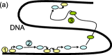
Figure 1: (a) Search scenario with 3 states. (b) Energy profile and switching rates between states.

We start the analysis by considering diffusion along the DNA in the 1D interval $0\leq x\leq L$ ($x$ is the DNA contour length) with switching between state 1 and 2. The target is located at $x=0$ and can only be found in state 1. To derive an expression for the MFPT, we use the sojourn times $t_{nm}(x)$ a particle spends in state $n$ ($n=1,2,3$) when it started in state $m=1,2$ at a DNA position $x$. Because a TF attaches to the DNA at a random position $x$, when starting the search in state 3, the sojourn times do not depend on the initial position, and we have $t_{n3}=\tau_{n3}=const$. The times $\tau_{n3}$ are related to the spatially averaged sojourn times $\tau_{nm}=L^{-1}\int_{0}^{L}t_{nm}(x)dx$. Considering that a TF can only bind to the target in state 1, we have the relations $\tau_{13}=\tau_{12}$, $\tau_{23}=k_{12}/k_{21}\tau_{13}+1/k_{21}$ and $\tau_{33}=k_{23}/k_{32}\tau_{23}+1/k_{32}$. The coupled system of equations describing $t_{11}(x)$ and $t_{12}(x)$ is Reingruber and Holcman (2010) (we suppress the $x$ dependency)

$$\begin{array}[]{lll}D_{1}t_{11}^{\prime\prime}-k_{12}(t_{11}-t_{12})&=&-1\\ D_{2}t_{12}^{\prime\prime}-k_{21}(t_{12}-t_{11})-k_{23}(t_{12}-\tau_{12})&=&0\end{array}$$ (3)

with boundary conditions $t_{11}(0)=t_{11}^{\prime}(L)=t_{12}^{\prime}(0)=t_{12}^{\prime}(L)=0$. The remaining sojourn times $t_{2m}(x)$ and $t_{3m}(x)$ are $t_{2m}(x)={k_{12}}/{k_{21}}t_{1m}(x)+k_{21}^{-1}(1-\delta_{m1})$ and $t_{3m}(x)={k_{23}}/{k_{32}}t_{2m}(x)$. By integrating eq. 3 we further obtain the intuitive relation $\tau_{11}=\tau_{12}$. Hence, starting initially uniformly distributed in state $m$, the MFPT $\tau(m)=\tau_{1m}+\tau_{2m}+\tau_{3m}$ can be expressed in terms of $\tau_{11}$ only. In particular, starting in state 1, we have $\tau(1)=\tau_{11}(1+{k_{12}}/{k_{21}}+{k_{12}}{k_{23}}/({k_{21}}{k_{32}}))$.

Using the variables $\hat{x}={x}/{L}$, $l_{12}={k_{12}/(L^{2}}{D_{1}})$, $l_{21}={k_{21}/(L^{2}}{D_{2}})$ and $l_{23}={k_{23}/(L^{2}}{D_{2}})$, and the functions $v_{1}(\hat{x})=k_{12}\tau_{11}(x)$ and $v_{2}(\hat{x})=k_{12}\tau_{12}(x)$ ($v_{1}$ is the mean number of switchings between state 1 and 2), the solutions of eq. 3 are

$$\begin{array}[]{c}\begin{pmatrix}\displaystyle v_{1}(\hat{x})\\ v_{2}(\hat{x})\end{pmatrix}=\displaystyle\frac{l_{21}}{\xi_{2}}\left(\frac{\cosh(\sqrt{l_{12}}\mu_{2}(1-\hat{x}))}{\sqrt{l_{12}}\mu_{2}\sinh(\sqrt{l_{12}}\mu_{2})}-\frac{1}{l_{12}\mu_{2}^{2}}\right)\vec{e}_{2}\vspace{0.2cm}\\ \displaystyle-\frac{l_{21}}{\xi_{2}}\left(\frac{\cosh(\sqrt{l_{12}}\mu_{1}(1-\hat{x}))}{\sqrt{l_{12}}\mu_{1}\sinh(\sqrt{l_{12}}\mu_{1})}-\frac{1}{l_{12}\mu_{1}^{2}}\right)\vec{e}_{1}+v_{1}\,,\end{array}$$

where $\xi_{2}=\sqrt{\left(1+({l_{21}+l_{23}})/{l_{12}}\right)^{2}-4{l_{23}}/{l_{12}}}$, $\xi_{1}=-1+({l_{21}+l_{23}})/{l_{12}}$, $\mu_{1}^{2}=1+({\xi_{1}-\xi_{2}})/{2}$, $\mu_{2}^{2}=1+({\xi_{1}+\xi_{2}})/{2}$ and $\vec{e}_{1}^{\top}=({l_{12}}({\xi_{1}+\xi_{2}})/({2}{l_{21}}),1)$, $\vec{e}_{2}^{\top}=({l_{12}}({\xi_{1}-\xi_{2}})/({2}{l_{21}}),1)$. The average $v_{1}=\int_{0}^{1}v_{1}(\hat{x})d\hat{x}$ is

$$\begin{array}[]{lcr}\displaystyle v_{1}&=&\displaystyle\frac{\xi_{2}-\xi_{1}}{2\xi_{2}}\left(\sqrt{l_{12}}\frac{\coth(\sqrt{l_{12}}\mu_{2})}{\mu_{2}}-\frac{1}{\mu_{2}^{2}}\right)\vspace{0.1cm}\\ &&\displaystyle+\frac{\xi_{1}+\xi_{2}}{2\xi_{2}}\left(\sqrt{l_{12}}\frac{\coth(\sqrt{l_{12}}\mu_{1})}{\mu_{1}}-\frac{1}{\mu_{1}^{2}}\right)\,.\end{array}$$ (8)

Because $\xi_{1}$, $\xi_{2}$, $\mu_{1}$ and $\mu_{2}$ are all independent of $L$, $v_{1}$ depends on $L$ only via $l_{12}$. The relevant physical parameters are $L$, $k_{12}$, $k_{21}$, $k_{23}$, $k_{32}$, $D_{1}$ and $D_{2}$. However, to facilitate our further discussion, we shall now characterize the rates $k_{12}$, $k_{21}$ and $k_{23}$ by the detaching probability $q={k_{23}}/({k_{21}+k_{23}})$ to switch from state 2 to 3 ($p=1-q$ is the probability to switch from state 2 to 1) and the lengths $l_{s1}=\sqrt{{D_{1}}/{k_{12}}}$ and $l_{s2}=\sqrt{{D_{2}}/({k_{21}+k_{23}})}$, corresponding to the average sliding distances in state 1 and 2 before switching. The spatially averaged search time $\tau\approx\tau(1)$ is

$$\tau=v_{1}\left(\frac{l_{s1}^{2}}{D_{1}}+\frac{l_{s2}^{2}}{pD_{2}}+\frac{1}{k_{32}}\frac{q}{p}\right)\,.$$ (9)

Before detaching and switching to state 3, a TF stays bound to the DNA for an average time $\tau_{DNA}=k_{23}^{-1}+k_{12}^{-1}p/q$, and the overall ratio of the mean time bound to the DNA to the mean time spent in state 3 is

$$r=k_{32}\tau_{DNA}=\frac{k_{32}l_{s1}^{2}}{D_{2}}\left(\frac{p}{q}\frac{D_{2}}{D_{1}}+\frac{l_{s2}^{2}}{ql_{s1}^{2}}\right)\,.$$ (10)

When switching between state 1 and 2 is fast and diffusion in state 1 is negligible compared to state 2 ($D_{1}\ll D_{2}$), then the diffusion constant with which a TF appears to slide along the DNA is

$$D_{a}\approx\frac{D_{2}}{1+{k_{21}}/{k_{12}}}=\frac{D_{2}}{1+pD_{2}l_{s1}^{2}/(D_{1}l_{s2}^{2})}\,.$$ (11)

When the parameters $L$, $D_{2}$ and $k_{32}$ are given, we shall now study how the search process depends on $l_{s1}$, $l_{s2}$, $q$ and $D_{1}$. Modulating these parameters can be a way to regulate gene expression. Because a TF moves in state 2 in a smooth potential, we consider that $D_{2}$ is comparable the 3D diffusion constant. In contrast, in state 1, the TF interacts with individual bp and the effective diffusion constant is much reduced and can be written as $D_{1}=D_{2}e^{-\chi}$, where $\chi>0$ depends on the binding energy profile. For a single sliding state, $\chi$ is related to the variance of the binding energy Slutsky and Mirny (2004); Malherbe and Holcman (2010). In general, $\chi$ depends on the DNA sequences and therefore on the position along the DNA, however, we consider a constant average value here. We later on show that the search is not much sensitive to $\chi$ variations in x, as long as $\chi$ is not too large. We now proceed with the asymptotic analysis in the regime where $\kappa={l_{s1}^{2}}/{l_{s2}^{2}}\ll 1$ and $q\ll 1$. The condition $\kappa\ll 1$ avoids a redundant search in state 1 where diffusion is slow. As long as switching between state 1 and 2 is fast compared to the time $k_{32}^{-1}$ spent in state 3, the limit $q\ll 1$ avoids too frequent detaching from the DNA that would increase the search time. Under the condition that $\kappa\ll 1$ and $q\ll 1$, we have the asymptotic $\xi_{1}\approx-\left(1-\kappa\right)$, $\xi_{2}\approx 1+\kappa(1-2q)$, $\mu_{1}^{2}\approx\kappa q$, $\mu_{2}^{2}\approx 1+\kappa$ and $v_{1}\approx{L}/{l_{s1}}(1+\sqrt{{\kappa}/{q}})$. Using these expressions in eq. 9 and eq. 10, we find

$$\tau \approx \sqrt{\frac{L^{2}}{D_{2}k_{32}}}\left(1+\sqrt{\frac{\kappa}{q}}\right)\left(\frac{e^{\chi}}{\alpha}+\frac{1}{\alpha\kappa}+\alpha q\right)\,,$$ (12)

$$r \approx \frac{e^{\chi}}{\alpha^{2}q}+\frac{1}{\alpha^{2}q\kappa}\,,$$ (13)

where $\alpha=\sqrt{{D_{2}}/({l_{s1}^{2}k_{32}})}$. When $\alpha$ and $\chi$ are fixed, the minimum of $\tau(q,\kappa)$ as a function of $\kappa$ and $q$ is achieved for $(\kappa_{min},q_{min})=(\sqrt{{2}/({\alpha e^{\chi}})},\alpha^{-2}\kappa_{min}^{-1})$, and

$$\displaystyle\tau_{min} = \displaystyle\sqrt{\frac{L^{2}}{D_{2}k_{32}}}\left(1+\sqrt{\frac{2\alpha}{e^{\chi}}}\right)^{2}\frac{e^{\chi}}{\alpha}\,.$$ (14)

$$r_{min} = 1+\sqrt{{2e^{\chi}}/{\alpha}}.$$ (15)

For ${e^{\chi}}/{\alpha}\ll 1$, the asymptotic expansion is $\tau_{min}\approx 2\sqrt{{L^{2}}/({D_{2}k_{32}})}(1+\sqrt{{2e^{\chi}}/{\alpha}})$, showing that $\tau_{min}$ does not depend exponentially on $\chi$ in that regime. We now compare our results with the ones for a single sliding state: when a TF alternates only between state 1 and 3 with rates $k_{13}$ and $k_{31}$ (the intermediate state 2 is absent), we find from eq. 8 that $\tilde{v}_{1}=\sqrt{l_{13}}=\sqrt{{L^{2}}/({D_{1}k_{13}})}$, and for the search time we recover the expression $\tilde{\tau}=\sqrt{{L^{2}}/({D_{1}k_{13}})}(k_{13}^{-1}+k_{31}^{-1})$ Malherbe and Holcman (2010); Elf et al. (2007); Slutsky and Mirny (2004); Meroz et al. (2009). When $k_{31}$ is fixed, the minimum $\tilde{\tau}_{min}=2\sqrt{{L^{2}}/({D_{1}k_{31}})}$ is achieved for $k_{13}=k_{31}$, and $r$ is always one at the minimum with a single sliding state, which is not any longer the case in the two states sliding model.

We now proceed with some numerical estimations using parameters for E.coli bacteria: $L=2.4\times 10^{6}$bp (half the size of E. coli DNA, to compensate that the target is located at the boundary in our analysis), $k_{32}=(1.4\mu s)^{-1}$ Elf et al. (2007); Malherbe and Holcman (2010) and $D_{2}=2\mu m^{2}$, comparable to the 3D diffusion constant Elf et al. (2007). In Fig. 2a, we plot the minimum of $\tau$ as a function of $\chi$ and for various $l_{s1}=(0.5,1,3,5)$ (in units of bp). The case $l_{s1}=0.5$ can be considered as an effective description of a physical search process where a TF is bound and immobile in state 1 (similar to the scenario considered in Hu et al. (2008)): after switching back to state 2, the TF position in state 2 has changed only slightly in the range of a single bp (the average of the maximum diffusion length in state 1 is $2l_{s1}=2\sqrt{D_{1}/k_{12}}=1$). This position change can also be interpreted as the variability due to the unbinding process. The mean binding time $k_{12}^{-1}$ depends on the energy barrier $\Delta E$ (in units of $k_{B}T$) separating state 1 from 2. Comparing the Arrhenius formula $k_{12}=\xi e^{-\Delta E}$, where $\xi$ is an effective prefactor, with $k_{12}=D_{1}/l_{s1}^{2}=D_{2}e^{-\chi}/l_{s1}^{2}$, we identify $\chi=\Delta E$ and $\xi=D_{2}/l_{s1}^{2}$. Hence, for $l_{s1}$ small, the parameter $\chi$ is the binding energy, however, for large $l_{s1}$, $\chi$ is related to the variance of the binding energy landscape in state 1, as described in Zwanzig (1988); Slutsky and Mirny (2004); Malherbe and Holcman (2010).

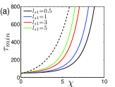
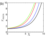
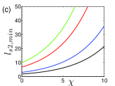
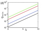
Figure 2: Optimal search process. Quantities are plotted as a function of $\chi$ and for various length $l_{s1}$. The parameter values are $L=2.4\times 10^{6}$bp, $k_{32}=(1.4ms)^{-1}$, $D_{2}=2\mu m^{2}s^{-1}$ and $D_{1}=D_{2}e^{-\chi}$. The dashed curve in (a) corresponds to the minimal time with a single sliding state. $\tau_{min}$ is given in sec.

Fig. 2a shows that $\tau_{min}$ is initially not very sensitive to $\chi$ until $\chi\sim\ln\alpha$ (for $l_{s1}=0.5$ we have $\ln\alpha\sim 6$). In contrast, with a single sliding state the minimum $\tilde{\tau}_{min}=2\sqrt{{L^{2}}/{(D_{2}k_{32})}}e^{\chi/2}$ (with $k_{31}=k_{32}$) increases exponentially with $\chi$ and quickly reaches much higher values (black dashed curve in Fig. 2a). Furthermore, within the two states sliding model, the novel feature is that the time ratio $r_{min}$ at the minimum is not constant but increases with $\chi$ (Fig. 2b). As a consequence, the experimental findings that a TF spends more time bound to the DNA compared to diffusing inside the nucleus Elf et al. (2007) is now compatible with an optimal search process. For example, for $l_{s1}=0.5$, the experimental results $\tau_{exp}\sim 350s$ and $r_{exp}\sim 5$ Elf et al. (2007) are compatible with a value $\chi\sim 8$ (Fig. 2a-b). Because diffusion in state 1 slows down as $\chi$ rises, the sliding distance $l_{s2,min}$ and the probability $q_{min}$ to switch from state 2 to state 3 increase, thereby reducing the probability of recurrently visiting the same DNA site in state 1 (Fig. 2c-d). Surprisingly, a larger detaching probability $q_{min}$ does not lead to a higher fraction of time spent in state 3, which is counter intuitive ($r_{min}$ increases, Fig. 2b).

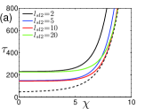
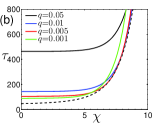
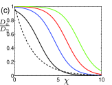
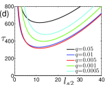
Figure 3: (a) Search time $\tau$ (in sec) for $l_{s1}=0.5$ and $q=0.01$. The dashed line is the minimum of $\tau$. (b) $\tau$ for $l_{s1}=0.5$ and $l_{s2}=10$. (c) Apparent diffusion constant $D_{a}$ scaled by $D_{2}$ for the situation in (a). The dashed line is the diffusion constant $D_{1}/D_{2}=e^{-\chi/2}$ for a model with a single sliding state. (d) Search time $\tau$ for $\chi=7.5$ showing a minimum.

To study the impact of increasing the binding strength in state 1, while the motion in state 2 (interaction with DNA backbone) is not affected, we plotted $\tau$ as a function of $\chi$ (Fig. 3a-b) for $l_{s1}=0.5$ and various $l_{s2}$ and $q$ that are independent of $\chi$. This is in contrast with Fig. 2, where $\tau_{min}$ is achieved for values of $q_{min}$ and $l_{s2,min}$ that do depend on $\chi$ and $l_{s1}$. In Fig. 3c, we plot the apparent diffusion constant $D_{a}$ (sliding along the DNA) as a function of $\chi$, with parameters associated with panel a. $D_{a}$ decreases as $\chi$ increases, and for $\chi\sim 7$, we have $D_{a}\sim 0.4\mu m^{2}s^{-1}$, which is similar to measurements Elf et al. (2007). Within a single sliding state model, the 1D diffusion coefficient $D_{1}=D_{2}e^{-\chi/2}$ decreases much faster as function of $\chi$ compared to $D_{a}$ (dashed line in Fig. 3c). We conclude that experimental measurements of the apparent diffusion constant are compatible with much stronger binding energies in a two-state compared to a single state model. Finally, we show how $\tau$ is modulated by varying $q$ or $l_{s2}$ for $\chi=7.5$ (Fig. 3d).

To conclude, we showed here that the TF search time, characterized by switching between two states on the DNA, is considerably faster and less sensitive to binding energy fluctuations compared to a single 1D sliding state. Performing fast translocations (’hoppings’) of the order of 10bp in state 2 speeds up the search time by reducing a slow recurrent search in state 1. In our analysis, switching between state 1 and 2 is a common and necessary feature of the search mechanism, in contrast to scenarios, where it is induced at strong DNA binding sites Slutsky and Mirny (2004). State 2 further offers the possibility that a TF moves along the DNA by translation without the need to follow the double-helix rotation. Furthermore, since DNA promoter sequences are usually $\gtrsim 10$bps and even present in several copies Wunderlich and Mirny (2009); Lässig (2007), small translocations in state 2 are unlikely to overshoot the target region. We show that an optimal search in our switching model involves a larger time spent bound to the DNA compared to diffusing in the nucleus, in agreement with experimental findings Elf et al. (2007). Finally, we find that the search time is very sensitive to changes in the detaching probability $q$. Hence, changing the TF interaction with the DNA backbone via modifying the electrical properties of the TF or the DNA by phosphorylation, methylation or acetylation is an efficient way to modulate the search time, and ultimately the cellular response. Future works should clarify the impact of the binding energy fluctuations in state 1, and should analyze in details the 3D dynamics, for example by considering DNA coiling Lomholt et al. (2009). Moreover, in eukaryotes, the compact DNA structure Lieberman-Aiden et al. (2009) and possible nuclear transport mechanism Shav-Tal and Gruenbaum (2009) might as well be critical. Nevertheless, we expect that our results derived here remain a good approximation as long as subsequent attaching positions to the DNA are well separated compared to the average distance a TF slides along the DNA before detaching (around 100bp), and the time spent in 3D is approximately exponentially distributed, both of which are widely used and accepted in the literature.

Acknowledgement: this research is supported by an ERC starting grant.

References

- Von Hippel and Berg (1989) P. Von Hippel and O. Berg, J. Biolog. Chemistry 264, 675 (1989).
- Halford and Marko (2004) S. Halford and J. Marko, Nucleic Acids Res. 32, 3040 (2004).
- Wang et al. (2006) Y. Wang, R. H. Austin, and E. Cox, Phys. Rev. Lett. 97, 048302 (2006).
- Blainey et al. (2006) P. Blainey, A. van Oijen, A. Banerjee, G. Verdine, and X. Xie, Proc Natl Acad Sci USA 103, 5752 (2006).
- Elf et al. (2007) J. Elf, G. Li, and X. Xie, Science 316, 1191 (2007).
- Riggs et al. (1970) A. D. Riggs, S. Bourgeois, and M. Cohn, J. Mol. Biol. 53, 401 (1970).
- Slutsky and Mirny (2004) M. Slutsky and L. Mirny, Biophys. J. 87, 4021 (2004).
- Zwanzig (1988) R. Zwanzig, Proc. Natl. Acad. Sci. USA 85, 2029 (1988).
- Gerland et al. (2002) U. Gerland, J. Moroz, and T. Hwa, Proc. Natl Acad. Sci. USA 99, 12015 (2002).
- Winter et al. (1981) R. B. Winter, O. Berg, and P. von Hippel, Biochemistry 20, 6961 6977 (1981).
- Kalodimos et al. (2004) C. Kalodimos, N. Biris, A. Bonvin, M. Levandoski, M. Guennuegues, R. Boelens, and R. Kaptein, Science 305, 386 (2004).
- Hu et al. (2008) L. Hu, A. Grosberg, and R. Bruinsma, Biophys. J. 95, 1151 (2008).
- Doering (2000) C. Doering, Lecture Notes in Physics: Stochastic Processes in Physics, Chemistry, and Biology 557, 316 (2000).
- Doering and Gadoua (1992) C. Doering and J. Gadoua, Phys Rev Lett. 69, 2318 (1992).
- Reingruber and Holcman (2009) J. Reingruber and D. Holcman, Phys. Rev. Lett. 103, 148102 (2009).
- Malherbe and Holcman (2010) G. Malherbe and D. Holcman, Phys. Lett. A 374, 466 (2010).
- Lomholt et al. (2009) M. Lomholt, B. van den Broek, S. Kalisch, G. Wuite, and R. Metzler, Proc Natl Acad Sci USA 106, 8204 (2009).
- Berg and Ehrenberg (1982) O. Berg and M. Ehrenberg, Biophys. Chem. 15, 41 (1982).
- Lomholt et al. (2005) M. Lomholt, T. Ambjörnsson, and R. Metzler, Phys. Rev. Lett. 95, 260603 (2005).
- Coppey et al. (2004) M. Coppey, O. Bénichou, R. Voituriez, and M. Moreau, Biophys. J. 87, 1640 (2004).
- Bénichou et al. (2009) O. Bénichou, Y. Kafri, M. Sheinman, and R. Voituriez, Phys. Rev. Lett. 103, 138102 (2009).
- Reingruber and Holcman (2010) J. Reingruber and D. Holcman, J. Phys.: Condens. Matter 22, 065103 (2010).
- Meroz et al. (2009) Y. Meroz, I. Eliazar, and J. Klafter, J. Phys. A: Math. Theor. 42, 434012 (2009).
- Wunderlich and Mirny (2009) Z. Wunderlich and L. Mirny, Trends Genet. 25, 434 (2009).
- Lässig (2007) M. Lässig, BMC Bioinformatics 8 Suppl 6 (2007).
- Lieberman-Aiden et al. (2009) E. Lieberman-Aiden, N. van Berkum, L. Williams, M. Imakaev, T. Ragoczy, A. Telling, I. Amit, B. Lajoie, P. Sabo, M. Dorschner, et al., Science 326, 289 (2009).
- Shav-Tal and Gruenbaum (2009) Y. Shav-Tal and Y. Gruenbaum, Biology Rep. pp. 1–29 (2009).