Bogoliubov-de Gennes study of trapped spin-imbalanced unitary Fermi gases

Abstract

It is quite common that several different phases exist simultaneously in a system of trapped quantum gases of ultra-cold atoms. One such example is the strongly-interacting Fermi gas with two imbalanced spin species, which has received a great amount of attention due to the possible presence of exotic superfluid phases. By employing novel numerical techniques and algorithms, we self-consistently solve the Bogoliubov de-Gennes equations, which describe Fermi superfluids in the mean-field framework. From this study, we investigate the novel phases of spin-imbalanced Fermi gases and examine the validity of the local density approximation (LDA), which is often invoked in the extraction of bulk properties from experimental measurements within trapped systems. We show how the validity of the LDA is affected by the trapping geometry, number of atoms and spin imbalance.

Keywords: Fermi gas, Fulde-Ferrel-Larkin-Ovchinnikov state

1 Introduction

Interest in spin-imbalanced Fermi superfluids dates back over a half century to the appearance of the Bardeen-Cooper-Schrieffer (BCS) theory. Several pioneers theoretically considered the fate of a superconductor in the presence of magnetic impurities which could disrupt the spin balance [1, 2, 3, 4] prescribed by BCS. In the ensuing decades the BCS picture has emerged as an important paradigm in many branches of physics [5], such as nuclear physics, quantum chromodynamics, and ultra-cold atoms. The ultra-cold atoms, in particular, provide a highly controllable clean system to investigate the effect of spin imbalance on the nature of fermionic pairing. Over the past few years, experiments on polarized Fermi gases at Rice University [6, 7, 8], MIT [9, 10, 11, 12] and ENS [13] have stimulated a flurry of theoretical activity. These efforts represent an important area within the general goal of emulating complicated many-body systems using cold atoms.

All cold atom experiments are necessarily performed in the presence of trapping potentials that hold the atoms together in an inhomogeneous environment. In order to extract the bulk properties of the system (e.g, the equations of state) from measurement on a trapped sample, a local density approximation (LDA) is employed to account for the effects of the trapping potential. The LDA states that the system can be treated locally as a part of an infinite system. In other words, on a length scale which is short in comparison to the spatial variation of the external potential, the external potential $V_{{\rm ext}}({\bf r})$ essentially acts as an offset to the chemical potential. In practice, one defines a local chemical potential $\mu({\bf r})=\mu-V_{{\rm ext}}({\bf r})$, with $\mu$ being the global chemical potential. In the context of cold atoms, the LDA is often an accurate approximation when there are no phase boundaries present. However, because of the large change in the density which occurs from the center to the edge of the trap, there is often more than one phase present and care needs to be taken in application of the LDA. This is especially true at phase boundaries where the LDA usually fails. Even in the circumstances where there is only one phase present in the trap, corrections to the LDA become crucial when the number of particles in the sample is small and finite-size effects are significant [14].

The trapped polarized Fermi gas represents just such a system — in all experimental observations, phase separation between a region with vanishing spin population and one with finite spin population has been observed. The purpose of this paper is to examine the validity of the LDA as the particle number and aspect ratio of the trap is changed. To this end we employ the Bogoliubov-de Gennes (BdG) equations [15], which is a powerful mean-field tool particularly suitable for inhomogeneous Fermi superfluids, and has been recently adopted by many to study trapped ultra-cold Fermi gases [16, 17, 18, 19, 20].

In a recent paper [21] we analyzed discrepancies observed in pioneering experiments on polarized fermionic superfluids [9, 10, 6, 7] which appear to center on physics arising when the containing trap is highly elongated. In our analysis we found that as the trap becomes increasingly elongated, the solutions of the BdG show a tendency towards metastable behavior which could lead to the observation of states which are not necessarily the ground state. However we also observed that one class of solutions with structure similar to the LDA solution was consistently the lowest in energy within our analysis. Our conclusions have since been confirmed by similar calculations [22] using a density functional formulation [23] which is more sophisticated than the BdG and accounts for quantum fluctuations and interactions within the normal fluid. In this paper we focus on this class of solutions and examine how well such solutions match those obtained from the LDA approximation as a function of particle number and trap aspect ratio.

The content of the paper is organized as follows. In Sec. 2, we present the BdG formulation and describe the numerical techniques used to solve the BdG equations. In Sec. 3 we discuss our results for a relatively small number of particles and for different trapping geometry. In Sec. 4, we focus on a very elongated cigar-like trap but vary the number of atoms. Finally, a concluding remark is presented in Sec. 5.

2 The Bogoliubov De-Gennes treatment

2.1 Formulation

We consider a gas of spin-polarized fermionic atoms interacting through a contact potential ($g\sum_{i<j}\delta^{3}(\vec{r}_{i}-\vec{r}_{j})$) and confined to a harmonic trap defined in cylindrical coordinates $(\rho,\phi,z)$ by $V_{\rm ext}(\rho,z)=\frac{m}{2}(\omega_{\bot}^{2}\rho^{2}+\omega_{z}^{2}z^{2})$ with axial and radial frequencies denoted by ($\omega_{z},\omega_{\bot})$. We work at unitarity $(a_{s}\rightarrow\infty)$ and within a cigar-shaped trap with aspect ratio $\alpha=\omega_{\bot}/\omega_{z}$. This system of $N=N_{\uparrow}+N_{\downarrow}$ atoms interacting through contact interaction is described by a Hamiltonian $\hat{H}=\int d\vec{R}\,(H_{0}+H_{I})$ with non-interacting $H_{0}$ and interacting $H_{I}$ portions given by:

$$H_{0}(\vec{R}) = \sum_{\sigma}\psi_{\sigma}^{\dagger}({-\frac{\hbar^{2}}{2m}\nabla^{2}+V_{\rm ext}\left(\rho,z\right)-\mu_{\sigma}})\psi_{\sigma}\,,$$

$$H_{I}(\vec{R}) = -g\,\psi_{\uparrow}^{\dagger}(\vec{R})\psi_{\downarrow}^{\dagger}(\vec{R})\psi_{\downarrow}(\vec{R})\psi_{\uparrow}(\vec{R})\,,$$ (1)

where $\psi_{\sigma}(\vec{R})$ represents the fermionic field operators, $m$ the mass and $\mu_{\sigma}$ the chemical potential of atomic species with spin $\sigma$. The coupling constant is defined as $g=\frac{4\pi\hbar^{2}a}{m}$. Henceforth, we work in trap units for which: $m=\omega_{z}=\hbar=k_{B}=1$. This implies that energies will be measured in units of $\hbar\omega_{z}$, lengths in units of $l_{0}=\sqrt{\frac{\hbar}{m\omega_{z}}}$ and temperature ($T$) in units of $\hbar\omega_{z}/k_{B}$ .

The Hamiltonian (1) will be treated within the mean-field BdG approximation for which there are many excellent references [15, 24, 25]. Here we simply state the BdG equations for the pair wave functions $u_{j}(\vec{R})$ and $v_{j}(\vec{R})$ which decouple $\hat{H}$:

$$\left[\begin{array}[]{cc}{\cal H}_{\uparrow}^{s}-\mu_{\uparrow}&\Delta(\vec{R})\\ \Delta(\vec{R})&-{\cal H}_{\downarrow}^{s}+\mu_{\downarrow}\end{array}\right]\left[\begin{array}[]{c}u_{j}\\ v_{j}\end{array}\right]=E_{j}\left[\begin{array}[]{c}u_{j}\\ v_{j}\end{array}\right],$$ (2)

In the above coupled set of equations, $u_{j}(\vec{R})$ and $v_{j}(\vec{R})$ are two components of the quasi-particle wavefunction associated with energy $E_{j}$. The single particle Hamiltonian ${\cal H}_{\sigma}^{s}$ is defined in our trap units by:

$${\cal H}_{\sigma}^{s}(\vec{R})=-{\nabla^{2}}/{2}+V_{\rm ext}+g\rho_{\bar{\sigma}}-\mu_{\sigma}$$ (3)

and includes the trapping potential, the chemical potential $\mu_{\sigma}$ and the Hartree mean-field potential is given by density $\rho_{\sigma}(\vec{R})=\langle\Psi_{\sigma}^{\dagger}(\vec{R})\Psi_{\sigma}(\vec{R})\rangle$. In accordance with fermionic commutation relations [15], the quasi-particle amplitudes are normalized as:

$$\int d\vec{R}\,|u_{j}(\vec{R})|^{2}+|v_{j}(\vec{R})|^{2}=1$$ (4)

and are related to the spin densities through :

$$\rho_{\uparrow}(\vec{R}) = \sum_{j=1}^{\infty}|u_{j}(\vec{R})|^{2}f\>(E_{j})$$

$$\rho_{\downarrow}(\vec{R}) = \sum_{j=1}^{\infty}|v_{j}(\vec{R})|^{2}f\>(E_{j}),$$ (5)

where $f(E)=1/(e^{E/k_{B}T}+1)$ is the Fermi-Dirac distribution function. In the unitary limit the Hartree terms $g\rho_{\bar{\sigma}}$ on the diagonal of Eq. (2) do not actually diverge but are unitarity limited [26]. How to incorporating the Hartree term in the unitarity limit is beyond the mean-field BdG formalism. For this reason we ignore this term in our calculations. The paring field or gap paramter is give by

$$\Delta(\vec{R})=g\langle\psi_{\uparrow}(\vec{R})\psi_{\downarrow}(\vec{R})\rangle=g\sum_{j}u_{j}(\vec{R})v^{*}_{j}(\vec{R})f(E_{j})$$ (6)

Since the Hartree terms are ignored in our analysis, Eqs. (2), (4) and (6) constitute a closed set of nonlinear equations which we solve self-consitently. However as presented above, our formulation has one problem which arises from a nasty side effect of the contact interaction. The contact interaction assumes wrongly that all states are scattered in the same way regardless of their incoming energy and consequently sums in contributions from collisions at arbitrarily high energy which creates an ultra-violet divergence. Hence the gap equation 6 needs to be properly regularized as we now discuss.

2.2 Regularizing the BdG equations

Due to the assumption of contact interaction, the gap $\Delta$ is a function of the center-of-mass coordinate of the pair, $\vec{R}$. To discuss the regularization, it is more convenient to re-introduce back the relative coordinate $\vec{r}$, with which the gap is defined as

$$\Delta(\vec{R},\vec{r})=\langle\psi_{\uparrow}(\vec{R}+{\vec{r}}/{2})\psi_{\downarrow}(\vec{R}-{\vec{r}}/{2})\rangle$$

which diverges as $\frac{\Delta(\vec{R})}{2\pi r}$ when $r\rightarrow 0$ [24]. To regularize Eq. (6), one simply subtracts off the $1/r$ divergence to obtain the regularized equation [24]:

$$\frac{\Delta(\vec{R})}{g}=\sum_{j}\,u_{j}(\vec{R})v_{j}^{*}(\vec{R})\,f(E_{j})-\frac{\Delta}{2\pi r}$$ (7)

In practice, the convergene of the sum above is quite slow and we discuss here a numerically efficient way of evaluating $\Delta(\vec{R})$ to sufficient accuracy without undue effort. First an energy cutoff $E_{c}$ is used to break the sum of Eq. (6) into two pieces as ff.

$$\frac{\Delta(\vec{R})}{g}=\sum_{E_{j}<E_{c}}\,u_{j}(\vec{R})v_{j}^{*}(\vec{R})f\>(E_{j})+\frac{\Delta_{c}(\vec{R})}{g}-\frac{\Delta(\vec{R})}{2\pi r}$$ (8)

The second term $\Delta_{c}(\vec{R})$ is an approximation to the sum above the cutoff using the LDA result for the pairing field [25] which can also be written as :

$$\frac{\Delta_{c}(\vec{R})}{g} = \frac{\Delta(\vec{R})}{(2\pi)^{3}}\int_{k_{c}}^{\infty}\frac{d^{3}k}{\sqrt{(\frac{k^{2}}{2}-\mu(\vec{R}))^{2}+\Delta^{2}}}$$ (9)

where $k_{c}$ is the momentum cutoff related to $E_{c}$. This leads to a computationaly efficient form of the gap equation:

$$\frac{\Delta(\vec{R})}{U_{\rm eff}(\vec{R})}=\sum_{E_{j}<E_{c}}\,u_{j}(\vec{R})v_{j}^{*}(\vec{R})\,f(E_{j}).$$ (10)

Here we have employed the identity:

$$\int_{0}^{\infty}\frac{d\vec{k}}{(2\pi)^{3}}\frac{e^{ikr}}{\frac{k^{2}}{2}}=\frac{1}{2\pi r}$$ (11)

to subsume the LDA approximation of the gap ($\Delta_{c}$) into an effective interaction defined by:

$$\frac{1}{U_{\rm eff}(\vec{R})}=\left[\frac{1}{g}-\int_{k_{c}}^{\infty}d^{3}k\left(\frac{1}{\sqrt{(\frac{k^{2}}{2}-\mu(\vec{R}))^{2}+\Delta^{2}}}-\frac{1}{\frac{k^{2}}{2}}\right)\right]$$ (12)

Below this cutoff $E_{c}$, the quasiparticle states are calculated exactly by solving Eqs. (2), (10) and (12) self-consistently along with the normalization conditions:

$$N_{\sigma} = \int\,\rho_{\sigma}(\vec{R})\,d\vec{R}$$ (13)

which conserve total particle number $N=N_{\uparrow}+N_{\downarrow}$ and overall polarization $P=(N_{\uparrow}-N_{\downarrow})/N$. The iterative solution of these equations is achieved using a modified Broyden’s approach [27] which is a nonlinear mixing scheme allowing the formation of polarized regions even if they were not present in the initial condition. In this scheme convergence was achieved when the root mean squared difference between $\Delta$ at different iterations was below some tolerance i.e., $\sqrt{\frac{\sum_{j}(\Delta_{i}^{j}-\Delta_{i+1}^{j})^{2}}{\sum\Delta_{i}^{j2}}}<tol$, where $j$ is the position index and $i$ represents the iteration number. We should point out that at unitarity this method is analogous to a descent technique where the step is optimized through the residuals stored from a few previous steps. As mentioned previouly we choose as our initial condition $\Delta_{\rm LDA}$, the LDA solution to the BdG equations. This is an important point becasue we found in previous work [21] that at larger particle numbers the solution of the BdG can be quite sensitive to the initial conditions.

2.3 Special features

We discretize using a linear triangular finite element mesh in the $\rho$-$z$ plane which anticipates that our results will retain the cylindrical symmetry of the confining potential $V_{ext}$. The accuracy of these calculations are controlled by the density of the trianglular mesh and the cut-off $E_{c}$ used in the hybrid scheme. Both of these are changed in successive solutions until the free-energy or relevant observable converges to a sufficient accuracy. Experience has taught us that this simple renormalization scheme typically converges when the cutoff is of the order $6E_{F}$ (where $E_{F}$ is the Fermi energy) which implies that the number of quasiparticle states to be directly calculated by Eq. (2) is about $6N$. Note that this puts a constraint on the density of the discretizing mesh. Thus, for moderate system sizes, we are still presented with a very large problem. For example, for $N\sim 10^{3}$ particles, one essentially needs to calculate $\sim 10^{5}$ quasiparticle states at each iteration.

One important consequence of our finite element discretization is that it yields sparse matrices which are suitable to massively parallel matrix computations. This is of key importance given that the slow convergence of the sum in Eq. (10) condemns us to calculate a very large number of quasi-particle states. This is true inspite of our efficient hybrid scheme, without which calculation would be prohibitive. It is immediately obvious that these difficulties will increase with the number of particles $N$, and will make the problem impractical for even moderate particle numbers without very careful formulation. In our case these difficulties are inescapable since the issues to be addressed occur in the presence of finite size effects and confinement. Hence it was crucial to develop the ability to perform calculations with realistic particle numbers because it is not a priori obvious how physical properties will scale with system size. At each iteration, we need to find a large number of eigenvalues and eigenfunctions for large matrices. To this end, we use a novel shift-and-invert scheme which we developed independently but is very similar to the one described in Ref. [28].

Briefly, the scheme involves partitioning the sought spectrum amongst groups of processors working independently. The size of the group is determined by the minimum number of processors with enough total memory to store the inverted matrix which is required for building the local Krylov basis. The main challenge here is bookkeeping to prevent over-counting of states and balancing the load amongst the processor groups. It is conceivable that this method could have issues in cases where the equations support huge degenerate subspaces. In our particular formulation we exploited cylindrical symmetry and parity along the long trap axis to reduce the problem. Consequently we only had to contend with accidental degeneracies. A good analysis of these issues may be found in Ref. [28] but a more thorough description of the numerical details will be presented elsewhere. However we note here that this parallelization scheme is very efficient on distriubted computing systems and scales easily to thousands of CPU’s which is as high as we have tested. Potentially it can be used to study much larger systems than we have reported here or in [21].

2.4 Validity of the BdG

We should devote a few lines here to comment on the validity of the BdG theory at unitarity becasue it is expected that quantum fluctuations and other effects due to the strong interactions could be significant in this regime. The main drawbacks of the BdG is that it fails to account for phase fluctations. At unitarity it has an additional disadvantage in that it also fails to account for interactions within the normal fluid which is unitarily limited [26]. However the BdG is widely expected to yield qualitatively reliable answers for two main reasons. First because of the finite size of these experiments, the trapped gas enjoys protection from fluctuations of arbitrarily low energy or of very long wavelengths. Secondly due to experimental evidence for superfluidity at unitarity, it is quite clear that interactions within the normal fluid are not so great that the order parameter cannot form or will be destroyed. Thus the failure to account for these effects is not expected to change the topology of the phase diagram but at most would slightly shift the phase boundaries. Since our purpose to examine the suitability of the LDA is qualitative, we are confident that the BdG can account for the essential physics. Nevertheless, due to the limitations within the BdG formalism, in particular the neglect of interaction in the normal fluid, our calculation fails to quantitatively locate position of the Clogston limit. In addition, it cannot be applied to study a system with extremely large polarization (i.e., $P\approx 1$) where the polaron physics will dominate [13, 29].

3 Results for $N=200$

In this section, we focus on a relatively small particle number of $N=200$. As we will show, the system is rather sensitive to the trap geometry. In the following, we first briefly discuss the case of a spherical trap with $\alpha=1$ and then concentrate on elongated cigar-like trapping potentials with $\alpha>1$ and then discuss them in detail.

3.1 Spherical trap

Liu et al. studied a spin-imbalanced Fermi gas confined in a spherical harmonic trap in Ref. [16]. To benchmark our work, we first did a series of calculations for this geometry and found our results in perfect agreement with those reported in Ref. [16]. In this case, even though we anticipate only cylindrical geometry, the density profiles always obey the spherical symmetry. Note that the authors of Ref. [16] solved the one-dimensional (1D) radial equation, hence the spherical symmetry of the cloud is automatically imposed. We refer the readers to Ref. [16] for details; here we give just a brief description of the key features. The density profiles indicate a phase-separation scenario: a fully paired BCS superfluid core at the trap center surrounded by a fully polarized shell composed of excess majority spins. A thin layer of partially polarized gas forms the interface between the superfluid core and the normal shell. In this intermediate regime, the minority density and the order parameter sharply drop to zero. Here and in other cases, we always found that the profile of the order parameter closely follows that of the density of the minority spin component. Furthermore, in this case, the LDA gives very good agreement with the full BdG calculation even for particle numbers as small as a few hundred.

3.2 Cigar trap

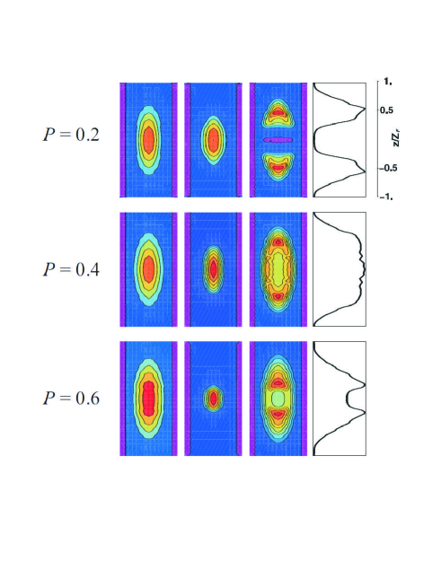
Figure 1: Density profile of the atomic clound for $N=200$ in an elongated trap with aspect ratio $\alpha=5$. The upper, middle and lower row are results from different polarizations $P=0.2$, 0.4 and 0.6, respectively. In each row, we have shown (from left to right) the column densities of the majority component $\int dx\,\rho_{\uparrow}$, the minority component $\int dx\,\rho_{\downarrow}$, their difference $\int dx\,(\rho_{\uparrow}-\rho_{\downarrow})$, and the axial spin density $n_{1D}(z)=\int dxdy\,(\rho_{\uparrow}-\rho_{\downarrow})$.

So far, all the experiments on spin-imbalanced Fermi gases have been performed in cigar-like traps with aspect ratio $\alpha>1$. For a given particle number, the 1D regime is eventually encountered in this geometry by increasing $\alpha$ and creates the possibility to study the 3D-1D dimensional crossover. Figure 1 illustrates several examples of the density profiles for $N=200$ atoms confined in a moderately elongated trap with $\alpha=5$ (this trap aspect ratio is close to what has been used in the MIT experiments). We find it convenient to express our results in terms of the Fermi energy $E_{\textit{F}}=(3N)^{1/3}\alpha^{2/3}$, central number density $(2E_{F})^{3/2}/(6\pi^{2})$, and the Thomas-Fermi radius along the $z$-axis $Z_{\textit{F}}=\sqrt{2E_{\textit{F}}}$ for a single species ideal Fermi gas of $N/2$ particles in a trap with identical parameters. The upper row of Fig. 1 shows the density profiles of a system with a relatively small polarization $P=0.2$. Here the axial spin density $n_{1D}(z)$ exhibits a double-horn structure and vanishes near $z=0$. This is a clear violation of the LDA which predicts that $n_{1D}$ should be flat topped [30]. Fig. 1 can be examined in tandem with Fig. 2 where for a closer inspection, we plot the densities and the order parameter along the axial and radial axis for two different polarizations. Fig. 2(a) displays results for $P=0.2$. The density profiles along the $z$-axis show clearly a phase separated three-region structure — moving from the center to the edge of the trap, we encounter a fully paired superfluid core, a partially paired intermediate region and a fully polarized normal gas, just like in the previous case of spherical trap. In stark contrast, the density profiles for the two components along the $\rho$-axis are completely overlapped. In fact, this matching of the radial profiles occur for $|z|\leq 0.1$. As a consequence, the axial spin density vanishes near $z=0$ as shown in the upper row of Fig. 1.

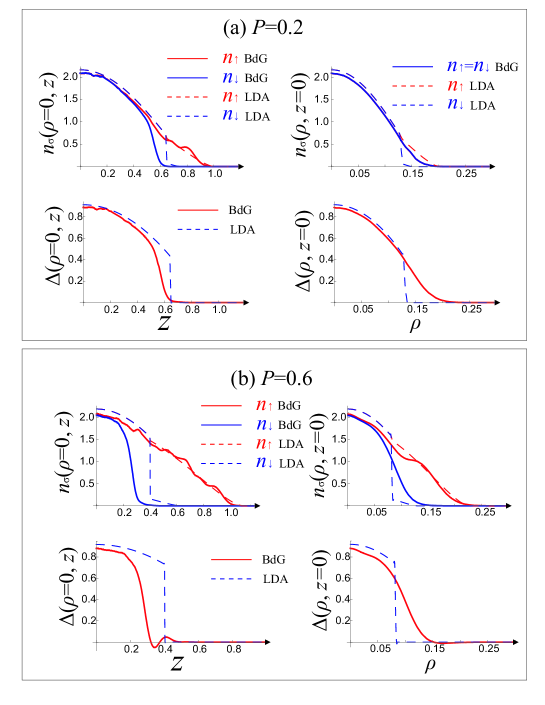
Figure 2: Density and order parameter profiles along the axial and radial axes in a cigar-like trap with $\alpha=5$ for two differnet polarizations: (a) $P=0.2$ and (b) $P=0.6$.

That the majority and minority densities overlap along the radial direction can be understood from an argument invoking the surface energy. When induced phase separation occurs, there is an accompanying surface energy associated with the interface between the two phases. The system will then try to minimize the interface in order to reduce the associated energy. For a cigar-like trap as we study here, the superfluid-normal gas interface area can be efficiently reduced if the two spin components match their densities radially. The authors of Ref. [31, 32] devised phenomenological theories to include the surface term variationally to explain the breakdown of the LDA observed in the Rice experiment [6, 7]. In our calculation, the surface energy is automatically included from the self-consistent BdG formulation [33].

As polarization increases, eventually it becomes energetically unfavorable to have this radial overlap. This is illustrated in Fig. 2(b) for $P=0.6$. Consequently, the axial spin density no longer vanishes near $z=0$ and the LDA becomes more accurate (see the middle and bottom rows of Fig. 1). In addition, it is quite noticeable that, particularly for large $P$, the minority component density has a steeper down turn along the axial axis than along the radial axis. Moreover, in the partially polarized intermediate region, the order parameter has a small oscillation along the axial axis, but not along the radial axis. Similar order parameter oscillations were also found in the spherical trap case [16]. This is a consequence of the proximity effect which, in the context of superconductor, occurs when a superconductor is in contact with a normal metal, the Cooper pairs from the superconductor diffuse into the normal component.

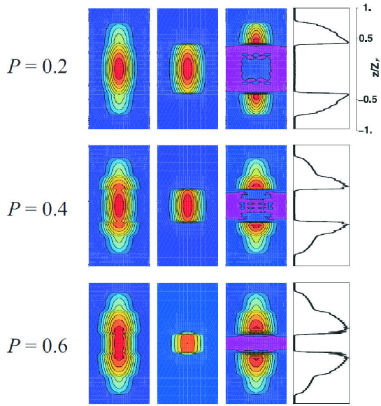
Figure 3: Same as in Fig. 1, but for $\alpha=50$.

Next, we keep $N$ fixed at 200 but increase the trap aspect ratio to $\alpha=50$ which represents a much more elongated cigar trap and close to what is used in the Rice experiment. A similar display of the column and axial spin density profiles for different polarization as in Fig. 1 is shown in Fig. 3. In this very elongated trap, the majority and minority components have their densities matched along the radial axis up to the highest polarization we have calculated which is $P=0.7$, and the minority component has a boxy-looking density profile. This further confirms that the system is able to greatly reduce the effective surface area between the normal state and the superfluid state in anisotropic cigar-like traps. Another marked feature for such an elongated trap is the prominent oscillations of the order parameter along the $z$-axis. As demonstrated in Fig. 4, these oscillations are quite generic features in such a trap with finite $P$. As $P$ increases, both the amplitude and the spatial extension of the oscillations increase. As shown in Fig. 4(b), at large polarizations, the axial length of the partially polarized intermediate region becomes comparable to or even larger than that of the BCS core. Accompanied by the oscillation in the order parameter, the density profiles (in particular, the minority density) also exhibit strong oscillations. Such oscillations are reminiscent of the FFLO pairing state predicted by Fulde, Ferrel, Larkin and Ovchinnikov [3, 4] in which the Cooper pairs possess finite momentum and the order parameter in the bulk develops sinusoidal oscillations that break the spatial translation symmetry.

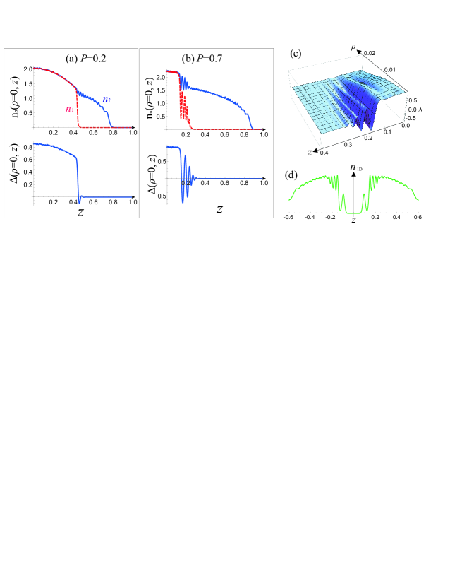
Figure 4: $\alpha=50$ for two different polarizations: (a) $P=0.2$ and (b) $P=0.7$. Same units as in Fig. 2. We do not show the radial density and order parameter profiles, which look more or less like those in Fig. 2(a). (c) The surface plot of the order parameter for the case of $P=0.7$ in the $\rho$-$z$ plane, showing strong oscillations with the nodes aligned along the radial direction. (d) The density oscillations for $P=0.7$ leave a strong signal in the doubly integrated axial spin density $n_{1D}$.

Our calculations also show that these axial oscillations are aligned along the radial axis, as shown in Fig. 4(c). We even intentionally started from an initial ansatz of $\Delta$ where the axial oscillations are present but with the nodes mis-aligned in the radial direction, the BdG iterations eventually converge to a state where the nodes are perfectly aligned radially. This radial alignment has important impact in detecting the oscillations in column density profiles where the densities are integrated along one radial axis: Due to the radial alignment, the oscillations are not washed out and can be easily observed, for example, in the doubly integrated axial spin density $n_{1D}$, as illustrated in Fig. 4(d).

It is interesting to compare our result with the recent work by Bulgac and Forbes [23] who, using a density functional theory, argued that the FFLO pairing phase occupies a larger phase space region than people previously thought for a 3D homogeneous system. The FFLO state found in Ref. [23] is also associated with large-amplitude density oscillations, particularly in the minority component. Another perspective on the order parameter oscillations and its potential connection with the FFLO phase is dimensionality. It is well known that the partially polarized phase with FFLO-like oscillations is prominently featured in the phase space of 1D systems [25, 34, 35]. That the reduced dimensionality favors such a state can be understood from the argument of Fermi surface nesting or alternatively from the cost of creating domain walls. The cigar-like traps used in our calculation mimic a quasi-1D system and may be the reason that we see pronounced oscillations in our calculation. If this latter explanation is correct, i.e., the partially polarized region featuring FFLO-like oscillations is due to the effective reduction of the spatial dimension, we then expect to see these oscillations diminish as $N$ is increased while the trap aspect ratio is fixed, which makes the system more 3D-like. To confirm this, we now turn to the next section where we keep $\alpha=50$ but vary the total particle number $N$.

4 Results for large particle numbers at $\alpha=50$

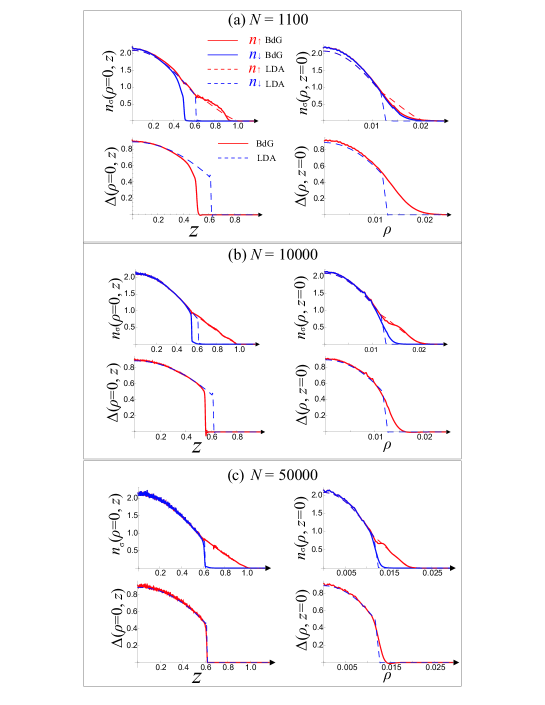
Figure 5: Density and order parameter profiles along the axial and the radial axis in a cigar-like trap with $\alpha=50$ for $P=0.3$ but different values of total particle number $N$. Same units as in Fig. 2.

We now consider a trapped system in a very elongated cigar trap with $\alpha=50$. Fig. 5 shows the density and order parameter along the axial and radial axis at a fixed polarization $P=0.3$ but different values of total particle number $N$. As one can clearly see, the oscillations in both the order parameter and the density profiles diminish as $N$ is increased and the LDA approximation becomes more and more accurate, which indicates that the FFLO-like region observed above for small $N$ does not represent a bulk 3D phase. Rather, it is a finite-size effect due to the effective reduction of the spatial dimension.

Nevertheless, we have discovered that as $N$ increases, the system exhibits a tendency towards metastability [21]. Numerically, by starting from different initial ans tze for the order parameter $\Delta(\vec{r})$, the BdG solution may converge to different final states. Our calculations show that among these different states, the one that closely resembles the LDA solution always has the lowest energy as long as $N$ is sufficiently large ($N\gtrsim 10^{4}$), but that there may exist several metastable states with energies just slightly larger that violate the LDA. The observed LDA-violating states at Rice are most likely these metastable states. Experimentally, whether the ground state or a metastable state will be realized may depend upon how the evaporative cooling procedure is implemented [36]. This has been confirmed very recently in a new experiment by Hulet group [37].

5 Conclusion

In conclusion, we have carried out a systematic study of a trapped spin-imbalanced Fermi gas in the unitary limit up to a total number $N\sim 10^{5}$ atoms. We study a class of solutions which has recently been identified as having the lowest energy [21, 22] through a self-consistently solution of the Bogoliubov-de Gennes equations using state-of-the-art numerical techniques. For a given set of trapping parameters, the LDA will eventually become accurate for sufficiently large $N$. However, the validity of the LDA is also sensitive to the trap geometry: Traps with small anisotropy favor the LDA. Our calculations show that for a relatively small number of atoms in a very elongated trapping potential, the system contains three phases: an unpolarized BCS phase, a partially polarized FFLO-like phase and a normal phase. That the FFLO region exists may be understood from the view point of reduced effective spatial dimension. As $N$ is increased while all other parameters remain fixed, the FFLO-like region eventually disappears. A detailed analysis of dimensional crossover will be reported in the future.

References

- [1] Clogston A M 1962 Phys. Rev. Lett. 9 266
- [2] Chandrasekhar B S 1962 Appl. Phys. Lett. 1 7
- [3] Fulde P and Ferrell R A 1964 Phys. Rev. 135 A550
- [4] Larkin A I and Ovchinnikov Y N 1965 Zh. Eksp. Teor. Fiz. 47 1136 [Sov. Phys. JETP 20 762 ]
- [5] Casalbuoni R and Nardulli G 2004 Rev. Mod. Phys. 76 263
- [6] Patridge G B et al. 2006 Science 311 492
- [7] Patridge G B et al. 2006 Phys. Rev. Lett. 97 190407
- [8] Liao Y-A et al. 2010 Nature 467 567
- [9] Zwierlein M W et al. 2006 Science 311 492
- [10] Zwierlein M W et al. 2006 Nature 442 54
- [11] Schunck C H et al. 2007 Science 316 867
- [12] Shin Y I et al. 2008 Nature 451 689
- [13] Nascimb ne S et al. 2009 Phys. Rev. Lett. 103 170402
- [14] Son D T 2007 preprint arXiv:0707.1851
- [15] De Gennes P 1989, Superconductivity of Metals and Alloys, (Addison-Wesley, Reading, MA)
- [16] Liu X-J, Hu H and Drummond P 2007 Phys. Rev. A 75 023614
- [17] Mizushima K, Machida K and Ichioka M 2005 Phys. Rev. Lett. 94, 060404
- [18] Ohashi Y and Griffin A 2005 Phys. Rev. A 72 013601
- [19] Kinnunen J, Jensen L M and T rm P 2006 Phys. Rev. Lett. 96 110403
- [20] Tezuka M, Yanase Y and Ueda M 2010 preprint arXiv:0811.1650v3
- [21] Baksmaty L O et al. 2011 Phys. Rev. A 83, 023604 (arXiv:1003.4488)
- [22] Pei J C, Dukelsky J and Nazarewicz W 2010 Phys. Rev. A 82, 021603
- [23] Bulgac A and Forbes M M 2008 Phys. Rev. Lett. 101 215301
- [24] G. Bruun, Y. Castin, R. Dum, and K. Burnett, Eur. Phys. J. D 7, 433-439 (1999)
- [25] Liu X-J, Hu H and Drummond P 2007 Phys. Rev. A 76 043605
- [26] Gupta S et al. 2003 Science 300 1723
- [27] Johnson D D 1988 Phys. Rev. B 38 12807
- [28] Zhang H et al. 2007 ACM Trans. Math. Software 33 9
- [29] Schirotzek A et al. 2009 Phys. Rev. Lett. 102 230402
- [30] De Silva T N and Mueller E J 2006 Phys. Rev. A 73 051602(R)
- [31] De Silva T N and Mueller E J 2006 Phys. Rev. Lett. 97 070402
- [32] Haque M and Stoof H T C 2007 Phys. Rev. Lett. 98 260406
- [33] Imambekov A et al. 2006 Phys. Rev. A 74, 053626
- [34] Orso G 2007 Phys. Rev. Lett. 98 070402
- [35] Hu H, Liu X-J and Drummond P 2007 Phys. Rev. Lett. 98 070403
- [36] Parish M M and Huse D 2009 Phys. Rev. A 80 063605
- [37] Hulet R G, private communication.