Unified Treatment of Hidden Markov Switching Models

Abstract

Many real-world problems encountered in several disciplines deal with the modeling of time-series containing different underlying dynamical regimes, for which probabilistic approaches are very often employed. In this paper we describe several such approaches in the common framework of graphical models. We give a unified overview of models previously introduced in the literature, which is simpler and more comprehensive than previous descriptions and enables us to highlight commonalities and differences among models that were not observed in the past. In addition, we present several new models and inference routines, which are naturally derived within this unified viewpoint.

1 Introduction

Several problems encountered in application areas such as finance, biology, speech analysis, control engineering, robotics, etc. require the modeling of time-series containing switching among different dynamics regimes (see Ephraim, (2002) for a review). For example, system fault diagnosis deals with detecting behavioural deviations from normality originated by failures in the system.

Such a modeling is often achieved by employing probabilistic approaches in which regime switching is described by a set of discrete hidden random variables, related by a first-order Markovian dependence. All such models, that we call hidden Markov switching models (HMSMs), can be viewed as extensions of the popular hidden Markov model Rabiner, (1989).

The wide interdisciplinary attention to this research area has produced many different HMSMs as well as different approaches and implementations of HMSMs of fundamentally similar structure, resulting in a dense literature from which extracting differences and commonalities among models is often challenging.

In this paper we provide a simple unified treatment of existing HMSMs, highlighting properties and connections that were not observed in previous review papers Ephraim, (2002); Gales and Young, (1993); Murphy, (2002); Ostendorf et al., (1996); Rabiner, (1989); Yu, (2010), and introduce novel extensions. Our exposition enables a deep understanding of the fundamental structure and relations of different approaches. This is achieved by using the framework of graphical models, which allows to easily define complex models by using a graphical representation and to derive efficient inference routines by visual inspection of the graph, avoiding complex algebraic manipulations.

2 Independence in Belief Networks

One of the fundamental tasks in probabilistic time-series modeling is the development efficient inference routines, which requires exploiting statistical independence relations among random variables. By using the framework of graphical models and, in particular, of belief networks Barber, (2011); Koller and Friedman, (2009); Pearl, (1988), statistical independence can be assessed by visual inspection of the graph, and therefore inference can be achieved without the need of algebraic manipulations. In this section, we introduce some basic definitions of the graphical model theory and explain two equivalent methods for assessing statistical independence. These methods form the basis for the derivations of the inference routines presented in the rest of the paper.

Figure 1: (a) Example of directed acyclic graph. The node $x_{3}$ is a collider in the path $x_{2},x_{3},x_{1}$, but it is a non-collider in the path $x_{2},x_{4},x_{3},x_{1}$. Adding a link from $x_{4}$ to $x_{1}$ would result in a cyclic graph. (b) Belief network representation of a hidden Markov model. Rectangular nodes indicate discrete variables, whilst oval nodes indicate discrete or continuous variables. Filled nodes indicate that the variables are observed.

Basic Graphical Model Definitions

A graphical model is a graph in which nodes represent random variables and (undirected or directed) links represent statistical dependencies among variables.
A path from node $x_{i}$ to node $x_{j}$ is a sequence of linked nodes connecting $x_{i}$ to $x_{j}$.
A node $x_{i}$ with a direct link towards $x_{j}$ is called parent of $x_{j}$. In this case, $x_{j}$ is called child of $x_{i}$.
An undirected path from $x_{i}$ to $x_{j}$ has a collider at $x_{k}$ if there are two arrows along the path pointing towards $x_{k}$. Notice that a node can be a collider in a path, but a non-collider in another path. For example, in Fig. 1 (a) $x_{3}$ is a collider in the path $x_{2},x_{3},x_{1}$, but it is a non-collider in the path $x_{2},x_{4},x_{3},x_{1}$.
A directed acyclic graph is a graph with no directed paths starting and ending at the same node. For example, the directed graph in Fig. 1 (a) is acyclic. Adding a link from $x_{4}$ to $x_{1}$ would make the graph cyclic.
A belief network is a directed acyclic graph in which each node $x_{i}$ has associated the conditional distribution $p(x_{i}|parents(x_{i}))$. The joint distribution of all nodes in the graph is given by the product of all conditional distributions

$$p(x_{1:D}\equiv x_{1},\ldots,x_{D})=\prod_{i=1}^{D}p(x_{i}|parents(x_{i})).$$

A node $x_{i}$ is called ancestor of a node $x_{j}$ if there exists a directed path from $x_{i}$ to $x_{j}$. In this case, $x_{j}$ is called descendant of $x_{i}$.

Assessing Statistical Independence

Method I. Given the sets of random variables ${\cal X},{\cal Y}$ and ${\cal Z}$, ${\cal X}$ and ${\cal Y}$ are statistically independent given ${\cal Z}$ (denoted with ${\cal X}\perp\!\!\!\perp{\cal Y}\,|\,{\cal Z}$) if all paths from any element of ${\cal X}$ to any element of ${\cal Y}$ are blocked. A path is blocked if at least one of the following conditions is satisfied

1. There is a non-collider in the path which is in the conditioning set ${\cal Z}$.

2. There is a collider in the path such that nor the collider nor any of its descendants is in ${\cal Z}$.

Method II. This method consists of converting the directed graph into an undirected one and then using the rules of independence for undirected graphs. This is achieved by the following steps:

1. Create the ancestral graph: remove any node which is neither in ${\cal X}\cup{\cal Y}\cup{\cal Z}$ nor an ancestor of a node in this set, together with any links in or out of such nodes.

2. Perform moralisation: add a link between any two nodes which have a common child. Remove arrowheads.

3. Use independence rules for undirected graphs: if all paths which join a node in ${\cal X}$ to one in ${\cal Y}$ pass through any member of ${\cal Z}$ then ${\cal X}\perp\!\!\!\perp{\cal Y}\,|\,{\cal Z}$.

3 Hidden Markov Model

We start our analysis with the Hidden Markov Model (HMM), which represents the basic model from which extensions will be derived. The HMM has a belief network representation given in Fig. 1 (b), in which the discrete or continuous (possibly multivariate) variable $v_{t}$ and the discrete variable $s_{t}$ represent respectively the observations and the underlying dynamics regime at time $t$. The joint distribution of all variables factorises as

$$p(v_{1:T},s_{1:T})=p(v_{1}|s_{1})p(s_{1})\prod_{t=2}^{T}p(v_{t}|s_{t})p(s_{t}|s_{t-1}).$$

We assume a homogeneous regime switching, parameterized by a vector $\tilde{\pi}$ and a matrix $\pi$ such that $p(s_{1})=\tilde{\pi}_{s_{1}}$ and $p(s_{t}|s_{t-1})=\pi_{s_{t}s_{t-1}}\textrm{ for }t>1$. For the case in which $v_{t}$ is a continuous variable, the distribution $p(v_{t}|s_{t})$ is commonly modelled as a Gaussian mixture.

There are three main properties that can limit the modelling accuracy of HMMs, namely

1. The strong independence assumption among observations $v_{t}\perp\!\!\!\perp v_{{\setminus t}\equiv v_{1},\ldots,v_{t-1},v_{t+1},\ldots,v_{T}}\,|\,s_{t}$, with consequent lack of smoothness in modeling the observations.

2. The weak modelling of the state-duration distribution: the probability of observing state $i$ for $d$ consecutive time-steps is implicitly given by the geometric distribution $\pi_{ii}^{d-1}(1-\pi_{ii})$, which is often inappropriate and encouraging too fast regime switching.

3. The limited power in modeling the observations when high noise is present. In particular, the HMMis unable to provide an estimate of the dynamics underlying noisy observations.

In the next sections we describe extensions of the HMM that overcome these limitations.

4 Extension of HMM to account for Dependency among Observations

A simple way of relaxing the strong independence assumption $v_{t}\perp\!\!\!\perp v_{\setminus t}\,|\,s_{t}$ in the HMM is to introduce Markovian dependence among the observations. In the belief network, this is represented by adding links from past to current observations, as shown in Fig. 2 (a) for the case of first-order dependence. For $k$-order dependence, the joint distribution can be written as,

$$p(v_{1:T},s_{1:T})=\prod_{t=1}^{T}p(v_{t}|s_{t},v_{t-k:t-1})p(s_{t}|s_{t-1}).$$

Models of this type include, for example, the Switching Autoregressive Model (SARM) in which $v_{t}=f(s_{t},v_{t-k:t-1})+\eta_{t}=\sum_{i=1}^{k}a^{s_{t}}_{i}v_{t-i}+\eta_{t}$ ($\eta_{t}$ being a Gaussian or Gamma noise vector) Hamilton, (1989, 1990, 1993), and extensions to a nonlinear interaction $f$ Susmel, (2000).

In the sequel, we describe efficient routines for solving the two most common inference problems in these models, namely the computation of $p(s_{t}|v_{1:T})$, known as smoothing, and the estimation of the most likely sequence of states $s^{*}_{1:T}=\mathop{\rm arg\,max}p(s_{1:T}|v_{1:T})$.

Figure 2: (a) Extension of the HMM to account for first-order Markovian dependence among the observations. (b) Ancestral moralized graph of the belief network in (a).

Smoothing with Parallel Routines

The estimation of $\gamma^{s_{t}}_{t}\equiv p(s_{t}|v_{1:T})$ can be obtained as

$$\gamma^{s_{t}}_{t} \propto p(s_{t},v_{1:T})=\underbrace{p(v_{t+1:T}|s_{t},\cancel{v_{1:t-k}},v_{t-k+1:t})}_{\beta^{s_{t}}_{t}}\underbrace{p(s_{t},v_{1:t})}_{\alpha^{s_{t}}_{t}},$$

where we have used the notation $p(v_{t+1:T}|s_{t},\cancel{v_{1:t-k}},v_{t-k+1:t})$ to emphasise the independence relation $v_{t+1:T}\perp\!\!\!\perp v_{1:t-k}\,|\,\{s_{t},v_{t-k+1:t}\}$. This relation can be assessed using any of the two methods explained in Section 2. For example, for $k=1$ we have $v_{t+1:T}\perp\!\!\!\perp v_{1:t-1}\,|\,\{s_{t},v_{t}\}$, which follows from

Method I:

All paths from (any element of) $v_{1:t-1}$ to (any element of) $v_{t+1:T}$ are blocked, as $v_{t+1:T}$ are reached by passing (1) from both $s_{t}$ and $v_{t}$, (2) from $s_{t}$ only, (3) from $v_{t}$ only (Fig. 2(a)). In cases (1) and (2), $s_{t}$ is a non-collider in the path which is in the conditioning set, and therefore condition 1. is satisfied. In case (3), $v_{t}$ is a non-collider in the path which is in the conditioning set, and therefore condition 1. is satisfied.

Method II:

The ancestral moralised graph is depicted in Fig. 2(b). All paths from $v_{1:t-1}$ to $v_{t+1:T}$ have to pass through an element of the conditioning set $s_{t}$ or $v_{t}$.

The terms $\alpha^{s_{t}}_{t}$ and $\beta^{s_{t}}_{t}$ can be recursively computed as follows

$$\alpha^{s_{t}}_{t} =p(v_{t}|s_{t},\cancel{v_{1:t-k-1}},v_{t-k:t-1})p(s_{t},v_{1:t-1})$$

$$=p(v_{t}|s_{t},v_{t-k:t-1})\sum_{s_{t-1}}p(s_{t}|s_{t-1},\cancel{v_{1:t-1}})p(s_{t-1},v_{1:t-1})$$

$$=p(v_{t}|s_{t},v_{t-k:t-1})\sum_{s_{t-1}}\pi_{s_{t}s_{t-1}}\alpha^{s_{t-1}}_{t-1},$$

$$\beta^{s_{t}}_{t} =\sum_{s_{t+1}}p(v_{t+1:T}|\cancel{s_{t}},s_{t+1},v_{t-k+1:t})p(s_{t+1}|s_{t},\cancel{v_{t-k+1:t}})$$

$$=\sum_{s_{t+1}}p(v_{t+2:T}|s_{t+1},v_{\cancel{t-k+1},{t-k+2:t+1}})p(v_{t+1}|s_{t+1},v_{t-k+1:t})\pi_{s_{t+1}s_{t}}$$

$$=\sum_{s_{t+1}}\beta^{s_{t+1}}_{t+1}p(v_{t+1}|s_{t+1},v_{t-k+1:t})\pi_{s_{t+1}s_{t}}.$$

For $k=1$ for example, the independence relation $s_{t}\perp\!\!\!\perp v_{1:t-1}\,|\,s_{t-1}$ can be demonstrated by noticing that all paths from $v_{1:t-1}$ to $s_{t}$ reach $s_{t}$ from (1) the non-collider $s_{t-1}$ which is in the conditioning set, (2) the collider $v_{t}$ which (together with all its descendants) is not in the conditioning set, (3) $s_{t+1}$ which imposes passing through a collider (e.g. $v_{t+1}$) which (together with all its descendants) is not in the conditioning set.

Notice that the $\alpha^{s_{t}}_{t}$ and $\beta^{s_{t}}_{t}$ recursions can be performed in parallel, after which $\gamma^{s_{t}}_{t}$ is computed. The computational cost of these recursions is $O(TS^{2})$ (without considering the cost of estimating terms such as $p(v_{t}|s_{t},v_{t-k:t-1})$). In order to avoid numerical overflow/underflow problems, computations are often preformed in log scale.

Smoothing with Sequential Routines

An alternative way of performing smoothing is to first compute the filtered distribution $\alpha^{s_{t}}_{t}\equiv p(s_{t}|v_{1:t})$ and then use this estimate to compute $\gamma^{s_{t}}_{t}\equiv p(s_{t}|v_{1:T})$ as follows
$\displaystyle\alpha^{s_{t}}_{t}$ $\displaystyle\propto p(v_{t}|s_{t},\cancel{v_{1:t-k-1}},v_{t-k:t-1})p(s_{t}|v_{1:t-1})$ $\displaystyle=p(v_{t}|s_{t},v_{t-k:t-1})\sum_{s_{t-1}}p(s_{t}|s_{t-1},\cancel{v_{1:t-1}})p(s_{t-1}|v_{1:t-1})$ $\displaystyle=p(v_{t}|s_{t},v_{t-k:t-1})\sum_{s_{t-1}}\pi_{s_{t}s_{t-1}}\alpha^{s_{t-1}}_{t-1},$ $\displaystyle\gamma^{s_{t}}_{t}$ $\displaystyle=\sum_{s_{t+1}}p(s_{t}|s_{t+1},v_{1:t},\cancel{v_{t+1:T}})p(s_{t+1}|v_{1:T})$ $\displaystyle=\sum_{s_{t+1}}\frac{p(s_{t+1}|s_{t},\cancel{v_{1:t}})p(s_{t}|v_{1:t})}{\sum_{\tilde{s}_{t}}p(s_{t+1}|\tilde{s}_{t},\cancel{v_{1:t}})p(\tilde{s}_{t}|v_{1:t})}\gamma^{s_{t+1}}_{t+1}$ $\displaystyle=\sum_{s_{t+1}}\frac{\pi_{s_{t+1}s_{t}}\alpha^{s_{t}}_{t}}{\sum_{\tilde{s}_{t}}\pi_{s_{t+1}\tilde{s}_{t}}\alpha^{\tilde{s}_{t}}_{t}}\gamma^{s_{t+1}}_{t+1},$ where the normalisation $p(v_{t}|v_{1:t-1})$ in the $\alpha^{s_{t}}_{t}$ recursion is obtained by summing the rhs of the above over all values of $s_{t}$. Notice that we are not making use of the observations after the $\alpha^{s_{t}}_{t}$ have been computed. These routines do not require working in a log scale.

In the following sections, we will focus on the parallel smoothing approach and come back a sequential smoothing approach in Section 7.

Computing the Most Likely Sequence of Hidden Variables

If we define $\delta^{s_{t}}_{t}=\max_{s_{1:t-1}}p(s_{1:t},v_{1:t})$, the most likely sequence of hidden variables $s^{*}_{1:T}=\mathop{\rm arg\,max}_{s_{1:T}}p(s_{1:T}|v_{1:T})$ can be obtained with the following algorithm

$$\delta^{s_{1}}_{1}=p(s_{1},v_{1})=\alpha^{s_{1}}_{1}$$

$$\textrm{for }t=2,\ldots,T\hskip 5.69046pt\delta^{s_{t}}_{t}=p(v_{t}|s_{t},v_{t-k:t-1})\max_{s_{t-1}}\pi_{s_{t}s_{t-1}}\delta^{s_{t-1}}_{t-1},\hskip 8.5359pt\psi^{s_{t}}_{t}=\mathop{\rm arg\,max}_{s_{t-1}}\pi_{s_{t}s_{t-1}}\delta^{s_{t-1}}_{t-1}$$

$$s^{*}_{T}=\mathop{\rm arg\,max}_{s_{T}}\delta^{s_{T}}_{T},\hskip 8.5359pt\textrm{for }t=T-1,\ldots,1\hskip 5.69046pts^{*}_{t}=\psi^{s^{*}_{t+1}}_{t+1}$$

where the recursion for $\delta^{s_{t}}_{t}$ is obtained as the $\alpha^{s_{t}}_{t}$ recursion with the sum replaced by the max operator.

Artificial Data Example

In this section, we illustrate how the switching autoregressive model (SARM) can overcomes the limitation of the HMM in modeling the temporal structure of a continuous time-series. In this continuous case, the observations in the HMM are commonly modeled as mixture of $M$ Gaussians, for which the smoothed distributions are given by $\gamma^{s_{t},m_{t}}_{t}=p(v_{t+1:T}|s_{t},\cancel{m_{t}},\cancel{v_{1:t}})p(s_{t},m_{t},v_{1:t})$ with

$$\alpha^{s_{t},m_{t}}_{t} =p(s_{t},m_{t},v_{1:t})$$

$$=p(v_{t}|s_{t},m_{t},\cancel{v_{1:t-1}})p(m_{t}|s_{t},\cancel{v_{1:t-1}})\sum_{s_{t-1}}p(s_{t}|s_{t-1},\cancel{v_{1:t-1}})p(s_{t-1},v_{1:t-1})$$

$$=p(v_{t}|s_{t},m_{t})p(m_{t}|s_{t})\sum_{s_{t-1}}p(s_{t}|s_{t-1})\sum_{m_{t-1}}p(s_{t-1},m_{t-1}|v_{1:t-1}),$$

which has computational cost $O(TS(M+SM))$, and

$$\beta^{s_{t}}_{t} =p(v_{t+1:T}|s_{t})$$

$$=\sum_{s_{t+1}}p(v_{t+2:T}|\cancel{s_{t}},s_{t+1},\cancel{v_{t+1}})\sum_{m_{t+1}}p(v_{t+1}|\cancel{s_{t}},s_{t+1},m_{t+1})p(m_{t+1}|\cancel{s_{t}},s_{t+1})p(s_{t+1}|s_{t})$$

which has computational cost $O(TS^{2}M)$.

We generated a 200 time-step-long time-series, corresponding to a noisy sinusoid with switching frequency at $t=100$. The time-series with the correct segmentation represented by different colours is plotted on the top of Fig. 3.

We then learned the parameters of a HMM with observations modeled as mixtures of $M=3$ Gaussians, using an EM algorithm where the M-step updates are given by

$$\mu_{s_{t},m_{t}}=\frac{\sum_{t=1}^{T}v_{t}p(s_{t},m_{t}|v_{1:T},\Theta^{i-1})}{\sum_{t=1}^{T}p(s_{t},m_{t}|v_{1:T},\Theta^{i-1})}$$

$$\Sigma_{s_{t},m_{t}}=\frac{\sum_{t=1}^{T}(v_{t}-\mu_{s_{t},m_{t}})(v_{t}-\mu_{s_{t},m_{t}})^{\textsf{T}}p(s_{t},m_{t}|v_{1:T},\Theta^{i-1})}{\sum_{t=1}^{T}p(s_{t},m_{t}|v_{1:T})}$$

$$p(s_{1})=p(s_{1}|v_{1:T},\Theta^{i-1}),p(s_{t}|s_{t-1})=\frac{\sum_{t=2}^{T}p(s_{t-1:t}|v_{1:T},\Theta^{i-1})}{\sum_{t=2}^{T}\sum_{s_{t}}p(s_{t-1:t}|v_{1:T},\Theta^{i-1})}$$

$$p(m_{t}|s_{t})=\frac{\sum_{t=1}^{T}p(s_{t},m_{t}|v_{1:T},\Theta^{i-1})}{\sum_{t=1}^{T}\sum_{m_{t}}p(s_{t},m_{t}|v_{1:T},\Theta^{i-1})}.$$

The resulting segmentation is given in the middle of Fig. 3. As we can see, the HMM splits the time-series into two regimes, one corresponding to higher values and the other one corresponding to lower values of the time-series. It is clear from this example, that in order to obtain the desired segmentation more temporal structure needs to be encoded into the model. One solution would be to add a link from $m_{t-1}$ to $m_{t}$, which would give an $\alpha$ routine

$$\alpha^{s_{t},m_{t}}_{t} =p(s_{t},m_{t},v_{1:t})$$

$$=p(v_{t}|s_{t},m_{t},\cancel{v_{1:t-1}})\sum_{m_{t-1}}p(m_{t-1:t},s_{t},v_{1:t-1})$$

$$=p(v_{t}|s_{t},m_{t})\sum_{m_{t-1}}p(m_{t}|m_{t-1},s_{t},\cancel{v_{1:t-1}})\sum_{s_{t-1}}p(m_{t-1},s_{t-1:t},v_{1:t-1})$$

$$=p(v_{t}|s_{t},m_{t})\sum_{m_{t-1}}p(m_{t}|m_{t-1},s_{t})\sum_{s_{t-1}}p(s_{t}|s_{t-1},\cancel{m_{t-1}},\cancel{v_{1:t-1}})p(s_{t-1},m_{t-1},v_{1:t-1})$$

$$=p(v_{t}|s_{t},m_{t})\sum_{m_{t-1}}p(m_{t}|m_{t-1},s_{t})\sum_{s_{t-1}}p(s_{t}|s_{t-1})\alpha^{s_{t-1},m_{t-1}}_{t-1},$$

which has computational cost $O(TSM(S+M))$. This therefore would increase computational complexity considerably for complex time-series in which $M$ needs to be high. A less expensive alternative is to use a SARM, which. After learning the parameters similarly to the HMM case, SARMgives the desired segmentation as shown in the bottom of Fig. 3.

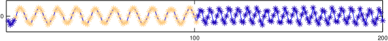
Figure 3: Top panel: the generated time-series up to the first 20 regime switches. Bottom panel: the sequence of (red) underlying and (gray) estimated regimes as $\mathop{\rm arg\,max}_{s_{t}}\sum_{c_{t}}\gamma^{s_{t},c_{t}}_{t}$. The intensity of the gray indicates the value $\max_{s_{t}}\sum_{c_{t}}\gamma^{s_{t},c_{t}}_{t}$ (darker colour means greater value).

5 Extension of the HMM to Model Explicitly the Regime-Duration Distribution

A way of overcoming the limitation of the implicit geometric regime-duration distribution of HMMs, is to define a different distribution by introducing extra random variables, at the price of increasing the computational cost of inference. This idea was first presented in Ferguson, (1980) and largely followed in the speech Murphy, (2002); Ostendorf et al., (1996); Rabiner, (1989) and statistics communities Guédon, (2003); Sansom and Thomson, (2001). There are two main ways to achieved this, which differ by using one or two sets of discrete hidden variables respectively. In the sequel we introduce them and discuss their relative properties.

In the exposition, we will pay particular attention to the calculation of the effective computational cost of the inference routines, with the goal of clarifying incorrectness and misunderstanding of the current literature.

5.1 Modelling the Regime-Duration Distribution with One Set of Duration-Count Variables

When using one set of discrete hidden variables $c_{1:T}$ for defining an explicit regime-duration distribution, we can think of two different approaches for modeling such variables. In the first approach, $c_{t}$ provides information about the time-step $\tau\geq t$ at which the current regime ends, which gives rise to decreasing duration-count variables within a regime. In the second approach, $c_{t}$ provides information about the time-step $\tau\leq t$ at which the current starts, which gives rise to increasing duration-count variables within a regime. These two approaches and their properties are discussed in detail in the sequel.

5.1.1 Decreasing Duration-Count Variables within a Regime

In the first approach to explicit modeling of the regime-duration distribution using decreasing duration-count variables within a regime, at a beginning of a regime $t$, $c_{t}$ indicates the number of time-steps (duration) spanned by the regime sampled according to a regime-duration distribution. At subsequent time-steps, the duration-count variables take progressively smaller values, until reaching value 1 at the end of the regime. More specifically, using the notation $\sigma_{t}=\{s_{t},c_{t}\}$, we define $p(\sigma_{1:T})=\prod_{t}p(\sigma_{t}|\sigma_{t-1})=\prod_{t}p(s_{t}|s_{t-1},c_{t-1})p(c_{t}|c_{t-1})$ with

$$p(s_{t}|s_{t-1},c_{t-1}) =\begin{cases}\pi_{s_{t}s_{t-1}}&\textrm{if }c_{t-1}\!=\!1,\\ \delta_{s_{t}=s_{t-1}}\hskip 7.68236pt&\textrm{if }c_{t-1}\!>\!1,\end{cases}$$

$$p(c_{t}|c_{t-1}) =\begin{cases}\rho_{c_{t}}&\textrm{if }c_{t-1}\!=\!1,\\ \delta_{c_{t}=c_{t-1}-1}&\textrm{if }c_{t-1}\!>\!1,\end{cases}$$

where $\delta$ is the Dirac delta and $\rho$ specifies the state-duration distribution. By considering a distribution that is zero outside the interval $\{d_{\min},\ldots,d_{\max}\}$, we can impose constraints on the minimum and (if $\pi_{ii}=0$) maximum duration allowed for a regime. We consider the case of $k$-order Markovian dependence among the observations, and therefore obtain a belief network representation of the model as in Fig. 4 (a) (for the case $k=1$).

Figure 4: HMSMs in which the regime-duration distribution is explicitly modelled using a set of discrete variables $c_{1:T}$ (a) as in Section 5.1.1 and (b) as in Section 5.1.2. In (b) the visible dependence across regimes (from time $t$ to time $t+1$) is cut (red dashed lines) ($c_{t+1}=1$ indicates the start of a new regime at time $t+1$).

Smoothing with parallel Routines

To estimate $\gamma^{\sigma_{t}}_{t}=p(\sigma_{t}|v_{1:T})\propto p(v_{t+1:T}|\sigma_{t},v_{t-k+1:t})p(\sigma_{t},v_{1:t})=\beta^{\sigma_{t}}_{t}\alpha^{\sigma_{t}}_{t}$ we can use a similar approach to the one described in Section 4. Specifically

$$\alpha^{\sigma_{t}}_{t} =p(v_{t}|s_{t},\cancel{c_{t}},\cancel{v_{1:t-k-1}},v_{t-k:t-1})p(\sigma_{t},v_{1:t-1})$$

$$=p(v_{t}|s_{t},v_{t-k:t-1})\sum_{\sigma_{t-1}}p(\sigma_{t}|\sigma_{t-1},\cancel{v_{1:t-1}})\alpha^{\sigma_{t-1}}_{t-1}$$

$$=p(v_{t}|s_{t},v_{t-k:t-1})\Big{\{}\delta_{c_{t}<d_{\max}}\alpha^{s_{t},c_{t}+1}_{t-1}+\rho_{c_{t}}\sum_{s_{t-1}}\pi_{s_{t}s_{t-1}}\alpha^{s_{t-1},1}_{t-1}\Big{\}},$$

where, by exploiting the fact that $c_{t}<d_{\max}$ implies that either $c_{t-1}=c_{t}+1,s_{t-1}=s_{t}$ or $c_{t-1}=1$, and the fact that $c_{t}=d_{\max}$ implies that $c_{t-1}=1$, we reduced the cost from $O(TS^{2}d^{2}_{\max})$ to $O(TS^{2}d_{\max})$. Further saving may be obtained by pre-computing $\sum_{s_{t-1}}\pi_{s_{t}s_{t-1}}\alpha^{s_{t-1},1}_{t-1}$, giving a complexity of $O(TS(S+d_{\max}))$. This cost is however more expensive than the cost $O(TS^{2})$ of the model in Section 4.

The term $\beta^{\sigma_{t}}_{t}$ can be obtained as follows

$$\!\beta^{\sigma_{t}}_{t} \!=\!\sum_{\sigma_{t+1}}p(v_{t+1:T}|\cancel{\sigma_{t}},\sigma_{t+1},v_{t-k+1:t})p(\sigma_{t+1}|\sigma_{t},\cancel{v_{t-k+1:t}})$$

$$\!=\!\sum_{\sigma_{t+1}}p(v_{t+2:T}|\sigma_{t+1},\cancel{v_{t-k+1}},v_{t-k+2:t+1})p(v_{t+1}|s_{t+1},\cancel{c_{t+1}},v_{t-k+1:t})p(\sigma_{t+1}|\sigma_{t})$$

$$\!=\!\delta_{c_{t}=1}\!\!\sum_{s_{t+1}}\!p(v_{t+1}|s_{t+1},v_{t-k+1:t})\pi_{s_{t+1}s_{t}}\sum_{c_{t+1}=d_{\min}}^{d_{\max}}\beta^{\sigma_{t+1}}_{t+1}\!\rho_{c_{t+1}}\!+\!\delta_{c_{t}>1}p(v_{t+1}|s_{t+1},v_{t-k+1:t})\beta^{s_{t},c_{t}-1}_{t+1},$$

where, by using the fact that $c_{t}=1$ implies change of regime at time $t+1$, whilst $c_{t}>1$ implies $c_{t+1}=c_{t}-1$, $s_{t+1}=s_{t}$, we have reduced the cost to $O(TSd_{\max})$.

Most Likely Sequence of Hidden Variables

With the notation $\delta^{\sigma_{t}}_{t}=\max_{\sigma_{1:t-1}}p(\sigma_{1:t},v_{1:t})$, the most likely sequence $\sigma^{*}_{1:T}=\mathop{\rm arg\,max}_{\sigma_{1:T}}p(\sigma_{1:T}|v_{1:T})$ can be obtained as

$$\delta^{\sigma_{1}}_{1}=p(\sigma_{1},v_{1})=\alpha^{\sigma_{1}}_{1}$$

$$\textrm{for }t=2,\cdots,T$$

$$\delta^{\sigma_{t}}_{t}=\begin{cases}p(v_{t}|s_{t},v_{t-k:t-1})\max[\delta^{s_{t},c_{t}+1}_{t-1},\rho_{c_{t}}\max_{s_{t-1}}\pi_{s_{t}s_{t-1}}\delta^{s_{t-1},1}_{t-1}]\hskip 1.9919pt&\textrm{if }c_{t}<d_{\max}\\ p(v_{t}|s_{t},v_{t-k:t-1})\rho_{c_{t}}\max_{s_{t-1}}\pi_{s_{t}s_{t-1}}\delta^{s_{t-1},1}_{t-1}&\textrm{otherwise }\end{cases}$$

$$\psi^{\sigma_{t}}_{t}=\begin{cases}\{\mathop{\rm arg\,max}_{s_{t-1}}\pi_{s_{t},s_{t-1}}\delta^{s_{t-1},1}_{t-1},1\}\hskip 1.9919pt&\textrm{if }\rho_{c_{t}}\max_{s_{t-1}}\pi_{s_{t}s_{t-1}}\delta^{s_{t-1},1}_{t-1}>\delta^{s_{t},c_{t}+1}_{t-1}\textrm{or }c_{t}=d_{\max}\\ \{s_{t},c_{t}+1\}&\textrm{otherwise }\end{cases}$$

$$\sigma^{*}_{T}=\mathop{\rm arg\,max}_{\sigma_{T}}\delta^{\sigma_{T}}_{T},\hskip 8.5359pt\textrm{for }t=T-1,\ldots,1\hskip 5.69046pt\sigma^{*}_{t}=\psi^{\sigma^{*}_{t+1}}_{t+1}.$$

Artificial Data Example

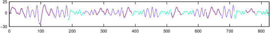
Figure 5: The generated time-series up to the first 20 regime switches, indicated by different colours.

There is considerable evidence in the literature that extensions of the HMM to explicitly model the regime-duration distribution give improvement in performance in several real-world problems such as handwriting and activity recognition, speech, MRI, financial time-series, rainfall time-series, and DNA analysis. Some specific examples can be found in Yu, (2010). In this section, we give a simple illustration of this property for the switching autoregressive model (SARM), using artificial data.

We generated a time-series from a 3-regime, 3-order SARM $v_{t}=\sum_{i=1}^{3}a^{s_{t}}_{i}v_{t-i}+\eta_{t}$ with

$$a^{1}=(1.8,-0.99,0),\hskip 4.26773pta^{2}=(1.65,-0.9,0.1),\hskip 4.26773pta^{3}=(1.8,-0.85,0);\hskip 9.95863pt\eta_{t}\sim{\cal N}(0,1).$$

The time-series contains 100 regime switches of type and duration uniformly sampled between 1 and 3 and between $d_{\min}=30$ and $d_{\max}=50$ respectively, giving a total length of $T=4004$. Notice that this problem is quite hard, since the autoregressive coefficients for the three regimes are similar. In Fig. 5 we show the generated time-series up to the first 20 regime switches, indicated by different colours.

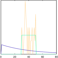
Figure 6: The empirical (orange), the GSARM (blue), and USARM  (green) regime-duration distributions for regime 2.

As a measure of segmentation error, we used the discrepancy between the correct and the estimated sequence of regimes (obtained as $\mathop{\rm arg\,max}_{s_{t}}\sum_{c_{t}}\gamma^{s_{t},c_{t}}_{t}$ for the case of smoothing). For the SARM with geometric regime-duration distribution (GSARM), we used the maximum likelihood value of the regime-switching distribution $\pi$ on the same sequence computed assuming that the other parameters and the segmentation are known. For the SARM with explicit regime-duration distribution (USARM), we used a uniform regime-duration distribution in the interval $\{30,\ldots,50\}$, and $\pi_{ii}=0,\pi_{ji}=1/(S-1),j\neq i$. In Fig. 6 we plot, for regime 2, the empirical regime-duration distribution of the time-series (orange) and the geometric (blue) and uniform (green) distributions used in the GSARM and USARM.

We have performed two experiments. In the first, the autoregressive coefficients and the Gaussian noise variance were assumed to be known, and therefore we measure difference in performance due to inference only. In this case, the GSARM gave a segmentation error of $0.16\%$ for the case in which smoothing was employed and of $0.31\%$ for the case in which the most likely sequence of regimes was estimated, whilst the USARM gave a smaller error of $0.07\%$ and $0.08\%$. In the bottom panel of Fig. 7 we show the sequence of (red) underlying and (gray) estimated regimes as $\mathop{\rm arg\,max}_{s_{t}}\sum_{c_{t}}\gamma^{s_{t},c_{t}}_{t}$. The intensity of the gray indicates the value $\max_{s_{t}}\sum_{c_{t}}\gamma^{s_{t},c_{t}}_{t}$ (darker colour indicates greater value). From this figure, we can observe that the GSARM is in general more uncertain about the regimes than the USARM, particularly for regime 2 to which portions of time-series belonging to other regimes are often assigned.

In the second experiment, the autoregressive coefficients and the Gaussian noise variance were assumed to be unknown, giving rise to a more difficult task. These parameters were estimated by the EM algorithm, using as initialisation

$$a^{1}=(0.8,-0.99,0),\hskip 4.26773pta^{2}=(-0.65,0.2,0.1),\hskip 4.26773pta^{3}=(0.9,-0.35,-0.3);\hskip 9.95863pt\eta_{t}\sim{\cal N}(0,100).$$

In this case, the GSARM gave a segmentation error of $0.15\%$ for the case in which smoothing was employed and of $0.28\%$ for the case in which the most likely sequence of regimes was estimated, whilst the USARM gave a smaller error of $0.07\%$ and $0.07\%$.

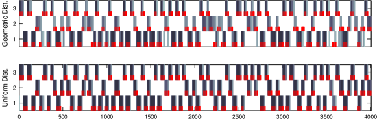
Figure 7: Top panel: the generated time-series up to the first 20 regime switches. Bottom panel: the sequence of (red) underlying and (gray) estimated regimes as $\mathop{\rm arg\,max}_{s_{t}}\sum_{c_{t}}\gamma^{s_{t},c_{t}}_{t}$. The intensity of the gray indicates the value $\max_{s_{t}}\sum_{c_{t}}\gamma^{s_{t},c_{t}}_{t}$ (darker colour means greater value).

5.1.2 Increasing Duration-Count Variables within a Regime

An alternative model for the duration-count variables $c_{1:T}$ to the one described in Section 5.1.1, would be to set $c_{t}=1$ at a beginning of a regime $t$, and define progressively increasing duration-count variables at subsequent time-steps within the regime. Specifically

$$p(s_{t}|s_{t-1},c_{t}) =\begin{cases}\pi_{s_{t}s_{t-1}}&\textrm{if }c_{t}\!=\!1,\\ \delta_{s_{t}=s_{t-1}}\hskip 7.68236pt&\textrm{if }c_{t}\!>\!1,\end{cases}$$

$$p(c_{t}|c_{t-1}) =\begin{cases}\lambda_{c_{t-1}}&\textrm{if }c_{t}\!=\!c_{t-1}+1,\\ 1-\lambda_{c_{t-1}}\hskip 7.68236pt&\textrm{if }c_{t}=1,\\ 0&\textrm{otherwise},\end{cases}$$

The relation between this model for $c_{1:T}$ and the one in Section 5.1.1 is given by

$$1-\lambda_{c_{t}}=\rho_{c_{t}}/\sum_{i=c_{t}}^{d_{\max}}\rho_{i}\,.$$

This can be seen as follows

$$\rho_{d} =p(\textrm{duration}=d)=(1-\lambda_{d})\underbrace{\lambda_{d-1},\ldots,\lambda_{2}\lambda_{1}}_{p(\textrm{duration}\geq d)}=(1-\lambda_{d})\sum_{i=d}^{d_{\max}}\rho_{i}\,.$$

This alternative model for $c_{1:T}$ is useful to derive efficient inference routines, for example, for the case of Markovian dependence among observations in which we want to define independence across regimes (these types of models are often called change-point models). This can be achieved by adding a link from $c_{t}$ to $v_{t}$ in the belief network (see Fig. 4 (b) for the case of order $k=1$). Indeed, in this case the variable $c_{t}$ encodes information about the time-step at which the current regime started and therefore about when to cut past dependence, i.e. $p(v_{t}|\cancel{v_{t-k:t-c_{t}}},v_{t-c_{t}+1:t-1},s_{t},c_{t})$, $k\geq c_{t}$. This would not be possible with the model of Section 5.1.1, in which at time $t$ information about when the current regime started is not available. Notice that, in this across-regimes independence case, it makes sense to have $\pi_{ii}\neq 0$. The $\alpha$ recursion is given by

$$\alpha^{\sigma_{t}}_{t} =p(v_{t}|\sigma_{t},\cancel{v_{1:t-k-1}},v_{t-k:t-1})p(\sigma_{t},v_{1:t-1})$$

$$=p(v_{t}|\sigma_{t},v_{t-k:t-1})\sum_{\sigma_{t-1}}p(\sigma_{t}|\sigma_{t-1},\cancel{v_{1:t-1}})\alpha^{\sigma_{t-1}}_{t-1}$$

$$=p(v_{t}|\sigma_{t},v_{t-k:t-1})\Big{\{}\delta_{c_{t}>1}\lambda_{c_{t}-1}\alpha^{s_{t},c_{t}-1}_{t-1}+\delta_{c_{t}=1}\sum_{c_{t-1}=d_{\min}}^{d_{\max}}(1\!-\!\lambda_{c_{t-1}})\sum_{s_{t-1}}\pi_{s_{t}s_{t-1}}\alpha^{\sigma_{t-1}}_{t-1}\Big{\}}\,,$$

where $p(v_{t}|\sigma_{t},v_{t-k:t-1})=p(v_{t}|\sigma_{t},v_{t-c_{t}+1:t-1})$ if $k\geq c_{t}$. The computational cost of this recursion is given by $O(TSd_{\max})$, namely the cost of the $\beta$ recursion in the previous model.

The $\beta$ recursion is obtained as follows

$$\beta^{\sigma_{t}}_{t} =\sum_{\sigma_{t+1}}p(v_{t+1:T}|\cancel{\sigma_{t}},\sigma_{t+1},v_{t-k+1:t})p(\sigma_{t+1}|\sigma_{t},\cancel{v_{t-k+1:t}})$$

$$=\sum_{\sigma_{t+1}}p(v_{t+2:T}|\sigma_{t+1},\cancel{v_{t-k+1}},v_{t-k+2:t+1})p(v_{t+1}|\sigma_{t+1},v_{t-k+1:t})p(\sigma_{t+1}|\sigma_{t})$$

$$=(1-\lambda_{c_{t}})\sum_{s_{t+1}}\!p(v_{t+1}|s_{t+1},c_{t+1}=1,v_{t-k+1:t})\pi_{s_{t+1}s_{t}}\beta^{s_{t+1},1}_{t+1}$$

$$+\delta_{c_{t}<d_{\max}}\lambda_{c_{t}}p(v_{t+1}|s_{t},c_{t+1}=c_{t}+1,v_{t-k+1:t})\beta^{s_{t},c_{t}+1}_{t+1}\,.$$

When pre-computing $\sum_{s_{t+1}}\!p(v_{t+1}|s_{t+1},c_{t+1}=1,v_{t-k+1:t})\pi_{s_{t+1}s_{t}}\beta^{s_{t+1},1}_{t+1}$, the computational cost of this recursion is given by $O(TS(S+d_{\max}))$, namely the cost of the $\alpha$ recursion in the previous model.

Figure 8: HMSMs in which the regime-duration distribution is explicitly modelled using two sets of discrete variables $c_{1:T},d_{1:T}$ as in Section 5.2. In (a) the visible dependence from time $1,\ldots,t$ to time $t+1,\ldots,T$ is cut (red dashed lines), since $c_{t}=1$ indicates the end of the regime at time $t$.

5.2 Modelling the Regime-Duration Distribution with Two Sets of Duration-Count Variables

In this section, we describe how to model the regime-duration distribution using two separate sets of discrete variables $d_{1:T}$ and $c_{1:T}$. The duration variable $d_{t}$ specifies the number of time-steps spanned by the observations forming the current regime, and takes a value sampled from a regime-duration distribution. The count variable $c_{t}$ is modelled similarly to Section 5.1.1, with the only difference that, at the beginning of a regime $t$, $c_{t}=d_{t}$ instead of being sampled from a regime-duration distribution. More specifically, by using the notation $\sigma_{t}=\{s_{t},d_{t},c_{t}\}$, we define $p(\sigma_{t}|\sigma_{t-1})=p(c_{t}|d_{t},c_{t-1})p(d_{t}|d_{t-1},c_{t-1})p(s_{t}|s_{t-1},c_{t-1})$ with

$$p(d_{t}|d_{t-1},c_{t-1}) =\begin{cases}\rho_{d_{t}}&\textrm{if }c_{t-1}\!=\!1,\\ \delta_{d_{t}=d_{t-1}}&\textrm{if }c_{t-1}\!>\!1,\end{cases}$$

$$p(c_{t}|d_{t},c_{t-1}) =\begin{cases}\delta_{c_{t}=d_{t}}&\textrm{if }c_{t-1}\!=\!1,\\ \delta_{c_{t}=c_{t-1}-1}&\textrm{if }c_{t-1}\!>\!1,\end{cases}$$

and $p(s_{t}|s_{t-1},c_{t-1})$ as in Section 5.1.1.

The variables $d_{t}$ and $c_{t}$ provide information about the time-steps in the past and future at which the current regime starts and ends. Therefore, unlike the previous models, this model can be used in the case of a non-Markovian visible dependence within a regime. This is expressed by the undirected links among the observations in the graphical model of Fig. 8 (a). Notice that, both visible independence across regimes (Fig. 8 (a)) or Markovian dependence across regimes (Fig. 8 (b)) can be assumed. In the first case, these models are usually called segmental HMMs.

In the sequel, we provide inference routines for the case in which independence is assumed.

Smoothing

In order to perform smoothing, we first compute terms of the type $\gamma^{s_{t},c_{t},1}_{t}=p(s_{t},d_{t},c_{t}=1|v_{1:T})$ for which the count variable takes value 1. If we define $\sigma^{1}_{t}\!=\!\{s_{t},d_{t},c_{t}\!=\!1\}$, we obtain

$$\gamma^{s_{t},d_{t},1}_{t}\propto\underbrace{p(v_{t+1:T}|s_{t},c_{t}\!=\!1,\cancel{d_{t},v_{1:t}})}_{\beta^{s_{t},1}_{t}}\underbrace{p(\sigma^{1}_{t},v_{1:t})}_{\alpha^{s_{t},d_{t},1}_{t}}.$$

The term $\alpha^{s_{t},d_{t},1}_{t}$ is estimated as follows,

$$\vspace{-3cm}\alpha^{s_{t},d_{t},1}_{t} =p(v_{t-d_{t}+1:t}|\sigma^{1}_{t},\cancel{v_{1:t-d_{t}}})p(\sigma^{1}_{t},v_{1:t-d_{t}})$$

$$=p(v_{t-d_{t}+1:t}|\sigma^{1}_{t})\sum_{s_{t-d_{t}},d_{t-d_{t}}}p(\sigma^{1}_{t}|\sigma^{1}_{t-d_{t}},\cancel{v_{1:t-d_{t}}})\alpha^{s_{t-d_{t}},d_{t-d_{t}},1}_{t-d_{t}}$$

$$=p(v_{t-d_{t}+1:t}|\sigma^{1}_{t})\rho_{d_{t}}\sum_{s_{t-d_{t}}}\pi_{s_{t}s_{t-d_{t}}}\underbrace{\sum_{d_{t-d_{t}}}\alpha^{s_{t-d_{t}},d_{t-d_{t}},1}_{t-d_{t}}}_{\hat{\alpha}^{s_{t-d_{t}},1}_{t-d_{t}}}$$

Whilst the complexity would appear to be $O(TS^{2}(d_{\max}-d_{\min}+1)^{2})$, by pre-computing $\hat{\alpha}^{s_{t-d_{t}},1}_{t-d_{t}}$ and $\tilde{\alpha}^{s_{t},1}_{t-d_{t}}=\sum_{s_{t-d_{t}}}\pi_{s_{t}s_{t-d_{t}}}\hat{\alpha}^{s_{t-d_{t}},1}_{t-d_{t}}$, we obtain a complexity of $O(TS(S+d_{\max}-d_{\min}+1))$ (without considering the complexity required to compute $q(v_{t-d_{t}+1:t}|\sigma^{1}_{t})$). Notice that this complexity is smaller than $O(TS^{2}d_{\max}^{2})$ and $O(TS^{2}d_{\max})$ (case $d_{\min}=1$) stated in Mitchell et al., (1995); Murphy, (2002); Rabiner, (1989); Yu and Kobayashi, (2003) for the same approach.

With the notation $\sigma^{k,1}_{t+k}=\{s_{t+k},d_{t+k}=k,c_{t+k}=1\}$, the term $\beta^{s_{t},1}_{t}$ can be estimated with the following recursion

$$\beta^{s_{t},1}_{t} =\!\sum_{s_{t+k},k}\!p(v_{t+1:T}|\sigma^{k,1}_{t+k},s_{t},c_{t}\!=\!1)p(\sigma^{k,1}_{t+k}|s_{t},c_{t}\!=\!1)$$

$$=\!\sum_{s_{t+k},k}\!p(v_{t+1:t+k}|\sigma^{k,1}_{t+k})\beta^{s_{t+k},1}_{t+k}\pi_{s_{t+k}s_{t}}\rho_{k},$$

which, by pre-computing $p(v_{t+1:t+k}|\sigma^{1,k}_{t+k})\beta^{s_{t+k},1}_{t+k}\rho_{k}$, has complexity $O(TS(S+d_{\max}-d_{\min}+1))$. Therefore, the $\alpha-\beta$ routines with separate duration-count variables are computationally convenient over common duration-count variables when $d_{\max}-d_{\min}+1\ll d_{\max}$.

Distributions of interest such as $p(s_{t},c_{t}|v_{1:T})$ can be estimated as

$$p(s_{t},c_{t}|v_{1:T})\propto\sum_{d=\max(d_{\min},c_{t})}^{d_{\max}}\beta^{s_{t},1}_{t+c_{t}-1}\alpha^{s_{t},d,1}_{t+c_{t}-1}$$

$$p(s_{t}|v_{1:T})\propto\sum_{\tau=t}^{t+d_{\max}-1}\sum_{d=\max(d_{\min},\tau-t+1)}^{d_{\max}}\beta^{s_{t},1}_{\tau}\alpha^{s_{t},d,1}_{\tau}\,.$$ (1)

The computational cost for $p(s_{t},c_{t}|v_{1:T})$ is given by $O(TSd_{\min}(d_{\max}-d_{\min}+1)+(d_{\max}-d_{\min})(d_{\max}-d_{\min}+1)/2)$. Indeed for $c_{t}=1,\ldots,d_{\min}$ we have $d_{\max}-d_{\min}+1$ summations to perform, whilst for $c_{t}=d_{\min}+1,\ldots,d_{\max}$ we have $d_{\max}-c_{t}+1$ summations to perform, which gives rise to $1+2+\ldots+d_{\max}-d_{\min}=(d_{\max}-d_{\min})(d_{\max}-d_{\min}+1)/2$.

Case $\pi_{ii}=0$.

In this case, it is more convenient to compute $p(s_{t}|v_{1:T})$, using the recursion for $\alpha^{s_{t},:,1}_{t}=\sum_{d_{t}}p(v_{t-d_{t}+1:t}|\sigma^{1}_{t})\rho_{d_{t}}\tilde{\alpha}^{s_{t},:,1}_{t-d_{t}}$ which has complexity $O(TS(S+d_{\max}-d_{\min}+1))$, and then calculate

$$p(s_{t}|v_{1:T})=\sum_{\tau<t}\beta^{*,s_{t},1}_{\tau}\alpha^{*,s_{t},:,1}_{\tau}-\beta^{s_{t},1}_{\tau}\alpha^{s_{t},:,1}_{\tau}\,.$$

Most Likely Sequence of Hidden Variables

If we define $\delta^{s_{t},d_{t},1}_{t}=\max_{s_{1:t-1},d_{1:t-1}}p(s_{1:t-1},d_{1:t-1},\sigma^{1}_{t},v_{1:t})$, then the most likely sequence of states, duration and count variables $s^{*}_{1:T},d^{*}_{1:T},c^{*}_{1:T}$ (under the assumptions $c_{T}=1$) can be obtained as

$$\textrm{for }t=1,\ldots,d_{\min}\hskip 5.69046pt\delta^{s_{t},d_{t},1}_{t}=\alpha^{s_{t},d_{t},1}_{t}$$

$$\left.\textrm{for }t=d_{\min}+1,\ldots,d_{\max}\right.\hskip 5.69046pt\delta^{s_{t},d_{t},1}_{t}=\left\{\begin{array}[]{l}\alpha^{s_{t},d_{t},1}_{t}\textrm{ if }d_{t}\geq t\\ p(v_{t-d_{t}+1:t}|\sigma^{1}_{t})\rho_{d_{t}}\max_{s_{t-d_{t}}}\pi_{s_{t}s_{t-d_{t}}}\max_{d_{t-d_{t}}}\delta^{s_{t-d_{t}},d_{t-d_{t}},1}_{t-d_{t}}\textrm{ if }d_{t}<t\\ \end{array}\right.$$

$$\textrm{for }t=d_{\max}+1,\ldots,T\hskip 5.69046pt\left.\begin{array}[]{l}\delta^{s_{t},d_{t},1}_{t}=p(v_{t-d_{t}+1:t}|\sigma^{1}_{t})\rho_{d_{t}}\max_{s_{t-d_{t}}}\pi_{s_{t}s_{t-d_{t}}}\max_{d_{t-d_{t}}}\delta^{s_{t-d_{t}},d_{t-d_{t}},1}_{t-d_{t}}\\ \psi^{s_{t},d_{t}}_{t}=\mathop{\rm arg\,max}_{s_{t-d_{t}},d_{t-d_{t}}}\pi_{s_{t}s_{t-d_{t}}}\delta^{s_{t-d_{t}},d_{t-d_{t}},1}_{t-d_{t}}\end{array}\right.$$

$$[s^{*}_{T},d^{*}_{T},c^{*}_{T}]=\left\{\begin{array}[]{l}\{\mathop{\rm arg\,max}_{s_{T},d_{T}}\delta^{s_{T},d_{T},1}_{T},1\}\textrm{ if contraint }c_{T}=1\\ \mathop{\rm arg\,max}_{s_{T},d_{T},c_{T}}\alpha^{s_{T},d_{T},c_{T}}_{T}\textrm{ if no contraint }c_{T}=1\\ \end{array}\right.$$

$$s^{*}_{T-d^{*}_{T}+c^{*}_{T}:T-1}=s^{*}_{T},d^{*}_{T-d^{*}_{T}+c^{*}_{T}:T-1}=d^{*}_{T},c^{*}_{T-d^{*}_{T}+c^{*}_{T}:T-1}=d^{*}_{T},\ldots,c^{*}_{T}+1$$

$$t=T-d^{*}_{T}+c^{*}_{T}-1,\hskip 2.84544pt\textrm{while }t>1\hskip 5.69046pt\left.\begin{array}[]{l}\{s^{*}_{t},d^{*}_{t},c^{*}_{t}\}=\{\psi^{s^{*}_{t+1},d^{*}_{t+1}}_{t+1},1\}\\ s^{*}_{t-d^{*}_{t}+1:t-1}=s^{*}_{t},\hskip 5.69046ptd^{*}_{t-d^{*}_{t}+1:t-1}=d^{*}_{t},\hskip 5.69046ptc^{*}_{t-d^{*}_{t}+1:t-1}=d^{*}_{t},\ldots,2\\ t=t-d^{*}_{t}\end{array}\right.$$

Sampling a Sequence of Hidden Variables from $p(\sigma_{1:T}|v_{1:T})$

Such samples can be obtained recursively by considering the factorisation $p(\sigma_{1:T}|v_{1:T})=p(\sigma_{T}|v_{1:T})\prod_{t=1}^{T-1}p(\sigma_{t}|\sigma_{t+1},v_{1:T})$. Suppose that, at time $t$, $c_{t}=1$ and we have sampled regime type $s_{t}$ and a duration $d_{t}$. Then, $s_{t-d_{t}+1:t-1}=s_{t}$, $d_{t-d_{t}+1:t-1}=d_{t}$ and $c_{t-d_{t}+1:t-1}=d_{t},\ldots,2,c_{t-k}=1$, so that effectively we need to sample $s_{t-d_{t}},d_{t-d_{t}}$ from the distribution $p(\sigma^{1}_{t-d_{t}}|\sigma_{t-d_{t}+1},v_{1:t},\cancel{v_{t+1:T}})$, which is given by

$$p(\sigma^{1}_{t-d_{t}}|\sigma_{t-d_{t}+1},v_{1:t+1}) =\frac{p(\sigma^{1}_{t-d_{t}},\sigma_{t-d_{t}+1},v_{1:t})}{p(\sigma_{t-d_{t}+1},v_{1:t})}$$

$$=\frac{\pi_{s_{t}s_{t-d_{t}}}\alpha^{s_{t-d_{t}},d_{t-k},1}_{t-d_{t}}}{\sum_{i}\pi_{s_{t}i}\sum_{l}\alpha^{i,l,1}_{t-d_{t}}}.$$

Note on Complexity.

It is clear from the complexity analysis described above that whether to use an approach with joint or separate duration-count variables depends on the specific goals and assumptions. If we are interested in estimating the most likely sequence of hidden variables or sampling a path only, then if $d_{\max}-d_{\min}+1\ll d_{\max}$, using separate variables is more convenient. However, when interested in distributions such as, then one has to take into account the extra cost incurred in computing these distributions.

6 Switching Linear Gaussian State-Space Models

In Sections 4 and 5, we have analysed how to improve the basic HMM model by enabling dependence among observations and by explicit modeling of the regime-duration distribution. In this section, we introduce another extension of the HMM called the Switching Linear Gaussian State-Space Model (SLGSSM), which enables a more accurate modeling of noisy and continuous observations and the reconstruction of the hidden dynamics underlying a sequence of noisy observations Mesot and Barber, (2007); Quinn et al., (2008); Zoeter, (2005).

The SLGSSM is defined by the following linear equations

$$h_{t}=A^{s_{t}}h_{t-1}+\eta^{h}_{t},\hskip 5.69046pt\eta^{h}_{t}\sim{\cal N}(\eta^{h}_{t};0,\Sigma^{s_{t}}_{H}),\hskip 1.42271pth_{1}\sim{\cal N}(h_{1};\mu^{s_{t}},\Sigma^{s_{t}}),$$

$$v_{t}=B^{s_{t}}h_{t}+\eta^{v}_{t},\hskip 5.69046pt\eta^{v}_{t}\sim{\cal N}(\eta^{v}_{t};0,\Sigma^{s_{t}}_{V}),$$

where the continuous hidden variables $h_{1:T}$ represents a hidden dynamics. The joint distribution of all variables factorizes as follows

$$p(v_{1:T},h_{1:T},s_{1:T})=p(v_{1}|h_{1},s_{1})p(h_{1}|s_{1})p(s_{1})\prod_{t=2}^{T}p(v_{t}|h_{t},s_{t})p(h_{t}|h_{t-1},s_{t})p(s_{t}|s_{t-1}).$$

Performing inference in the SLGSSM is intractable since, e.g., $p(h_{t}|s_{t},v_{1:t})$ is a Gaussian mixture with $S^{t-1}$ components. Several approximation schemes have been introduced over the years in order to deal with this intractability issue. For filtering, a successful method consists of employing a Gaussian collapsing procedure in a filtering routine on the line of the standard LGSSM predictor-corrector filtering routine. For smoothing, Barber, (2006) showed how, by introducing some approximations, it is possible to use Gaussian collapsing in a Rauch-Tung-Striebel style smoothing routine, obtaining improved accuracy over other approximation schemes.

7 Extension of SLGSSM with Explicit Regime-Duration Distribution

As in the classical HMM, the regime-duration distribution of the SLGSSM is implicitly geometric. Therefore the SLGSSM shares the same limitations of the HMM in this respect. In this section, we show how apply methods analogous to the ones described in Section 5 for explicitly modeling the regime-duration distribution of the SLGSSM.

We will use a Gaussian collapsing approximation method on the line of Barber, (2006). Extensions of the SLGSSM for defining an explicit duration distribution have also been studied in S. M. Oh and Dellaert, (2008). The authors introduce a set of duration-count variables $c_{1:T}$ as in Section 5.1.1, and use standard approximate inference methods for the SLGSSM in which the discrete hidden variables is a merged variable $\{c_{t},s_{t}\}$. Sparsity in the transition distribution of the merged variables is then used to reduce computational cost. The advantage of maintaining separate variables is to get insight into the problem and properties of the approach. As we will see, this will enables us to derive exact inference for the special case in which independence among observations is imposed.

7.1 Modeling State-Duration Distribution with One Set of Count-Duration Variables

In this section, we describe how define an explicit state-duration distribution for the SLGSSM by using one set of count-duration variables $c_{1:T}$ as in Section 5.1.

7.1.1 Decreasing Duration-Count Variables

The first approach is by modeling the duration-count variables as in Section 5.1.1, obtaining the belief network representation in Fig. 9 (a). In the sequel, we will describe how to perform smoothing in this model. Unlike the models explained in the previous sections, this will be achieved with a sequential approach that first computes the filtered distributions $p(h_{t},s_{t}|v_{1:t})$ and then uses this estimate to compute $p(h_{t},s_{t}|v_{1:T})$. This approach is preferable, since working in a log scale is not possible.

Figure 9: Extension of a sLGDS with duration-count variables.

Filtering

An approach to filtering is to form the following recursion for $p(h_{t}|\sigma_{t},v_{1:t})$

$$p(h_{t}|\sigma_{t},v_{1:t}) =\sum_{\sigma_{t-1}}p(h_{t}|\sigma_{t-1},s_{t},\cancel{c_{t}},v_{1:t})p(\sigma_{t-1}|\sigma_{t},v_{1:t})$$

$$=\delta_{c_{t}<d_{\max}}p(h_{t}|s_{t-1}=s_{t},c_{t-1}=c_{t}+1,s_{t},v_{1:t})p(s_{t-1}=s_{t},c_{t-1}=c_{t}+1|\sigma_{t},v_{1:t})$$

$$+\sum_{s_{t-1}}p(h_{t}|s_{t-1},c_{t-1}=1,s_{t},v_{1:t})p(s_{t-1},c_{t-1}=1|\sigma_{t},v_{1:t})\,.$$ (2)

In order to understand the complexity of this recursion, suppose for simplicity that $d_{\min}=1$. Then $p(h_{1}|\sigma_{1},v_{1})$ is a Gaussian and, from the recursion, we see that $p(h_{2}|\sigma_{2},v_{1:2})$ is a mixture of Gaussian with $S$ components. Therefore, in general, $p(h_{t}|\sigma_{t},v_{1:t})$ is a mixture of Gaussians with $S^{t-1}$ components as in the standard SLGSSM. In order to overcome, this exponential explosion of component with time, after estimating the recursion, we collapse the obtained mixture to a single Gaussian.

Below we describe how to compute each required term in the recursion.

Computing $p(h_{t}|\sigma_{t-1},s_{t},v_{1:t})$.

We have

$$p(h_{t}|\sigma_{t-1},s_{t},v_{1:t}) =\frac{p(v_{t},h_{t}|\sigma_{t-1},s_{t},v_{1:t-1})}{p(v_{t}|\sigma_{t-1},s_{t},v_{1:t-1})}$$

$$=\frac{p(v_{t}|\cancel{\sigma_{t-1}},s_{t},h_{t},\cancel{v_{1:t-1}})p(h_{t}|\sigma_{t-1},s_{t},v_{1:t-1})}{p(v_{t}|\sigma_{t-1},s_{t},v_{1:t-1})}$$

$$=\frac{p(v_{t}|s_{t},h_{t})\int_{h_{t-1}}p(h_{t-1:t}|\sigma_{t-1},s_{t},v_{1:t-1})}{p(v_{t}|\sigma_{t-1},s_{t},v_{1:t-1})}$$

$$=\frac{p(v_{t}|s_{t},h_{t})\int_{h_{t-1}}p(h_{t}|h_{t-1},\cancel{\sigma_{t-1}},s_{t},\cancel{v_{1:t-1}})p(h_{t-1}|\sigma_{t-1},\cancel{s_{t}},v_{1:t-1})}{p(v_{t}|\sigma_{t-1},s_{t},v_{1:t-1})}.$$

If we assume that $p(h_{t-1}|\sigma_{t-1},v_{1:t-1})$ is a Gaussian distribution with mean $\hat{h}_{t-1}^{t-1,\sigma_{t-1}}$ and covariance $P_{t-1}^{t-1,\sigma_{t-1}}$, by using the linear system equations defining the evolution of the continuous hidden variables we find that $p(h_{t}|\sigma_{t-1},s_{t},v_{1:t-1})$ is Gaussian with mean and covariance given by

$$\hat{h}_{t}^{t-1,\sigma_{t-1},s_{t}} =\langle h_{t}\rangle_{p(h_{t}|\sigma_{t-1},s_{t},v_{1:t-1})}=A^{s_{t}}\hat{h}_{t-1}^{t-1,\sigma_{t-1}}$$

$$P_{t}^{t-1,\sigma_{t-1},s_{t}} =\langle(h_{t}-h_{t}^{t-1,\sigma_{t-1},s_{t}})(h_{t}-h_{t}^{t-1,\sigma_{t-1},s_{t}})^{\textsf{T}}\rangle_{p(h_{t}|\sigma_{t-1},s_{t},v_{1:t-1})}$$

$$=A^{s_{t}}P_{t-1}^{t-1,\sigma_{t-1}}(A^{s_{t}})^{\textsf{T}}+\Sigma^{s_{t}}_{H}.$$

By using the linear system equations defining the observation-generation process we find

$$\langle v_{t}\rangle_{p(v_{t}|\sigma_{t-1},s_{t},v_{1:t-1})}=B^{s_{t}}\hat{h}_{t}^{t-1,\sigma_{t-1},s_{t}}$$

$$\langle(v_{t}-\langle v_{t}\rangle)(v_{t}-\langle v_{t}\rangle)^{\textsf{T}}\rangle_{p(v_{t}|\sigma_{t-1},s_{t},v_{1:t-1})}=B^{s_{t}}P_{t}^{t-1,\sigma_{t-1},s_{t}}(B^{s_{t}})^{\textsf{T}}+\Sigma^{s_{t}}_{V}$$

$$\langle(v_{t}-\langle v_{t}\rangle)(h_{t}-\hat{h}_{t}^{t-1,\sigma_{t-1},s_{t}})^{\textsf{T}}\rangle_{p(v_{t},h_{t}|\sigma_{t-1},s_{t},v_{1:t-1})}=B^{s_{t}}P_{t}^{t-1,\sigma_{t-1},s_{t}}.$$

By using the formula of Gaussian conditioning, we find that $p(h_{t}|\sigma_{t-1},s_{t},v_{1:t})$ is Gaussian with mean and covariance given by

$$\hat{h}_{t}^{t,\sigma_{t-1},s_{t}}=\hat{h}_{t}^{t-1,\sigma_{t-1},s_{t}}+K(v_{t}-B^{s_{t}}\hat{h}_{t}^{t-1,\sigma_{t-1},s_{t}})$$

$$P_{t}^{t,\sigma_{t-1},s_{t}}=P_{t}^{t-1,\sigma_{t-1},s_{t}}-KB^{s_{t}}P_{t}^{t-1,s_{t-1},s_{t},c_{t-1}}\,,$$

where $K=P_{t}^{t-1,\sigma_{t-1},s_{t}}(B^{s_{t}})^{\textsf{T}}(B^{s_{t}}P_{t}^{t-1,\sigma_{t-1},s_{t}}(B^{s_{t}})^{\textsf{T}}+\Sigma^{s_{t}}_{V})^{-1}$.

Computing $p(\sigma_{t-1}|\sigma_{t},v_{1:t})$.

We have

$$p(\sigma_{t}|v_{1:t}) =\frac{p(v_{t},\sigma_{t}|v_{1:t-1})}{p(v_{t}|v_{1:t-1})}$$

$$\propto\sum_{\sigma_{t-1}}p(v_{t},\sigma_{t-1:t}|v_{1:t-1})$$

$$=\sum_{\sigma_{t-1}}p(v_{t}|\sigma_{t-1},s_{t},v_{1:t-1})p(c_{t}|c_{t-1})p(s_{t}|\sigma_{t-1})p(\sigma_{t-1}|v_{1:t-1})$$

$$=\delta_{c_{t}<d_{\max}}p(v_{t}|s_{t-1}=s_{t},c_{t-1}=c_{t}+1,s_{t},v_{1:t-1})p(s_{t-1}=s_{t},c_{t-1}=c_{t}+1|v_{1:t-1})$$

$$+\sum_{s_{t-1}}p(v_{t}|s_{t-1},c_{t-1}=1,s_{t},v_{1:t-1})\rho_{c_{t}}\pi_{s_{t}s_{t-1}}p(s_{t-1},c_{t-1}=1|v_{1:t-1}),$$

where $p(v_{t}|\sigma_{t-1},s_{t},v_{1:t-1})=\frac{1}{\sqrt{\det P_{t}^{t-1,\sigma_{t-1},s_{t}}}}e^{-\frac{1}{2}(v_{t}-\hat{h}_{t}^{t-1,\sigma_{t-1},s_{t}})(P_{t}^{t-1,\sigma_{t-1},s_{t}})^{-1}(v_{t}-\hat{h}_{t}^{t-1,\sigma_{t-1},s_{t}})}$. Therefore

$$p(\sigma_{t-1}|\sigma_{t},v_{1:t}) =\frac{p(\sigma_{t-1:t}|v_{1:t})}{p(\sigma_{t}|v_{1:t})}$$

$$=\frac{p(v_{t},\sigma_{t-1:t}|v_{1:t-1})}{p(v_{t}|v_{1:t-1})p(\sigma_{t}|v_{1:t})}$$

$$=\frac{p(v_{t}|\sigma_{t-1},s_{t},v_{1:t-1})p(c_{t}|c_{t-1})p(s_{t}|\sigma_{t-1})p(\sigma_{t-1}|v_{1:t-1})}{p(v_{t}|v_{1:t-1})p(\sigma_{t}|v_{1:t})}\,.$$ (3)

Gaussian Collapsing.

We can collapse the mixture of $S$ Gaussians $p(h_{t}|\sigma_{t},v_{1:t})$ to a Gaussian by moment matching

$$\hat{h}_{t}^{t,\sigma_{t}} =\delta_{c_{t}<d_{\max}}p(s_{t-1}=s_{t},c_{t-1}=c_{t}+1|\sigma_{t},v_{1:t})\hat{h}_{t}^{t,s_{t},c_{t}+1,s_{t}}$$

$$+\sum_{s_{t-1}}p(s_{t-1},c_{t-1}=1|\sigma_{t},v_{1:t})\hat{h}_{t}^{t,s_{t-1},1,s_{t}}$$

$$P_{t}^{t,\sigma_{t}} =p(s_{t-1}=s_{t},c_{t-1}=c_{t}+1|\sigma_{t},v_{1:t})(P_{t}^{t,s_{t},c_{t}+1,s_{t}}+\hat{h}_{t}^{t,s_{t},c_{t}+1,s_{t}}(\hat{h}_{t}^{t,s_{t},c_{t}+1,s_{t}})^{\textsf{T}})$$

$$+\sum_{s_{t-1}}p(s_{t-1},c_{t-1}=1|\sigma_{t},v_{1:t})(P_{t}^{t,s_{t-1},1,s_{t}}+\hat{h}_{t}^{t,s_{t-1},1,s_{t}}(\hat{h}_{t}^{t,s_{t-1},1,s_{t}})^{\textsf{T}})-\hat{h}_{t}^{t,\sigma_{t}}(\hat{h}_{t}^{t,\sigma_{t}})^{\textsf{T}}.$$

The computational cost of this filtering recursion is $O(TS^{2}(d_{\max}-d_{\min}+1))$. However, notice that if we plug Eq. 3 into Eq. 2 we obtain

$$p(h_{t}|\sigma_{t},v_{1:t})$$

$$=\delta_{c_{t}<d_{\max}}p(h_{t}|s_{t-1}=s_{t},c_{t-1}=c_{t}+1,s_{t},v_{1:t})p(s_{t-1}=s_{t},c_{t-1}=c_{t}+1|\sigma_{t},v_{1:t})$$

$$+\frac{\rho_{c_{t}}}{p(v_{t}|v_{1:t-1})p(\sigma_{t}|v_{1:t})}\sum_{s_{t-1}}p(h_{t}|s_{t-1},c_{t-1}=1,s_{t},v_{1:t})p(v_{t}|s_{t-1},c_{t-1}=1,s_{t},v_{1:t-1})\pi_{s_{t}s_{t-1}}p(\sigma_{t-1}|v_{1:t-1})$$

Therefore one sum only over $s_{t-1}$ for all $c_{t}$ is required and the cost reduces to $O(T(S(d_{\max}-d_{\min}+1)+S))$.

Cut of dependence when changing regime.

Notice that in this model, we can introduce cut of dependence when changing regime by adding a link from $c_{t-1}$ to $h_{t}$ as in Fig. 9 (b), and therefore in principle without the need to use a modeling for $c_{1:T}$ as in Section 5.1.2. In this case

$$p(h_{t}|h_{t-1},s_{t},c_{t-1}) =\begin{cases}{\cal N}(h_{t};\mu^{s_{t}},\Sigma^{s_{t}})\hskip 16.21828pt&\textrm{if }c_{t-1}=1\\ {\cal N}(h_{t};A^{s_{t}}h_{t-1},\Sigma^{s_{t}}_{H})&\textrm{if }c_{t-1}>1\\ \end{cases}$$

Therefore, the filtering recursion becomes

$$p(h_{t}|\sigma_{t},v_{1:t}) =\sum_{\sigma_{t-1}}p(h_{t}|\sigma_{t-1},s_{t},\cancel{c_{t}},v_{1:t})p(\sigma_{t-1}|\sigma_{t},v_{1:t})$$

$$=\delta_{c_{t}<d_{\max}}p(h_{t}|s_{t-1}=s_{t},c_{t-1}=c_{t}+1,s_{t},v_{1:t})p(s_{t-1}=s_{t},c_{t-1}=c_{t}+1|\sigma_{t},v_{1:t})$$

$$+\sum_{s_{t-1}}p(h_{t}|\cancel{s_{t-1}},c_{t-1}=1,s_{t},\cancel{v_{1:t-1}},v_{t})p(s_{t-1},c_{t-1}=1|\sigma_{t},v_{1:t})$$

$$=\delta_{c_{t}<d_{\max}}p(h_{t}|s_{t-1}=s_{t},c_{t-1}=c_{t}+1,s_{t},v_{1:t})p(s_{t-1}=s_{t},c_{t-1}=c_{t}+1|\sigma_{t},v_{1:t})$$

$$+\frac{p(v_{t}|h_{t},s_{t}){\cal N}(h_{t};\mu^{s_{t}},\Sigma^{s_{t}})}{p(v_{t}|s_{t},c_{t-1}=1)}\sum_{s_{t-1}}p(s_{t-1},c_{t-1}=1|\sigma_{t},v_{1:t})$$

$$=\delta_{c_{t}<d_{\max}}\frac{p(v_{t}|s_{t},h_{t})\int_{h_{t-1}}{\cal N}(h_{t};A^{s_{t}}h_{t-1},\Sigma^{s_{t}}_{H})p(h_{t-1}|\sigma_{t-1},\cancel{s_{t}},v_{1:t-1})}{p(v_{t}|\sigma_{t-1},s_{t},v_{1:t-1})}$$

$$p(s_{t-1}=s_{t},c_{t-1}=c_{t}+1|\sigma_{t},v_{1:t})$$

$$+\frac{p(v_{t}|h_{t},s_{t}){\cal N}(h_{t};\mu^{s_{t}},\Sigma^{s_{t}})}{p(v_{t}|s_{t},c_{t-1}=1)}p(c_{t-1}\!=\!1|\sigma_{t},v_{1:t}).$$

From this recursion we see that $p(h_{t}|\sigma_{t},v_{1:t})$ is a mixture of Gaussian with $t$ components (and $p(h_{t}|v_{1:t})$ is a mixture of Gaussian with $Sd_{\max}t$ components). It is therefore feasible to perform inference without the collapsing approximation. However, as we will see below, it is computationally more convenient to use a modeling for $c_{1:T}$ as in Section 5.1.2, for which $p(h_{t}|v_{1:t})$ is a mixture of Gaussian with $Sd_{\max}$ components.

Smoothing

For smoothing we use the following recursion

$$p(h_{t}|\sigma_{t},v_{1:T}) =\sum_{\sigma_{t+1}}p(h_{t}|\sigma_{t:t+1},v_{1:T})p(\sigma_{t+1}|\sigma_{t},v_{1:T})$$

$$=\delta_{c_{t}=1}\sum_{\sigma_{t+1}}p(h_{t}|\sigma_{t:t+1},v_{1:T})p(\sigma_{t+1}|\sigma_{t},v_{1:T})$$

$$+\delta_{c_{t}>1}p(h_{t}|\sigma_{t},s_{t+1}=s_{t},c_{t+1}=c_{t}-1,v_{1:T})\overbrace{p(s_{t+1}=s_{t},c_{t+1}=c_{t}-1|\sigma_{t},v_{1:T})}^{1}\,.$$

Notice that in general $h_{t}\cancel{\perp\!\!\!\perp}c_{t+1}\,|\,\sigma_{t},s_{t+1},v_{1:T}$ since, for example, the path $c_{t+1},s_{t+2},v_{t+2},h_{t+2},h_{t+1},h_{t}$ is not blocked. However for $c_{t}>1$, $p(h_{t}|\sigma_{t},s_{t+1}=s_{t},c_{t+1}=c_{t}-1,v_{1:T})=p(h_{t}|\sigma_{t},v_{1:T})$.

Computing $p(h_{t}|\sigma_{t:t+1},v_{1:T})$.

$$p(h_{t}|\sigma_{t:t+1},v_{1:T}) =\int_{h_{t+1}}p(h_{t}|h_{t+1},\sigma_{t},s_{t+1},\cancel{c_{t+1}},v_{1:t},\cancel{v_{t+1:T}})p(h_{t+1}|\sigma_{t:t+1}v_{1:T})$$

$$\approx\int_{h_{t+1}}p(h_{t}|h_{t+1},\sigma_{t},s_{t+1},v_{1:t})p(h_{t+1}|\sigma_{t+1},v_{1:T}).$$ (4)

By using the linear system equations defining the evolution of the continuous hidden variables we find

$$\langle(h_{t+1}-\hat{h}_{t+1}^{t,i,j,l})(h_{t}-\hat{h}_{t}^{t,i,l})^{\textsf{T}}\rangle_{p(h_{t+1}|s_{t}=i,s_{t+1}=j,c_{t}=l,v_{1:t})}=A^{j}P_{t}^{t,i,l}.$$

Thus the joint covariance of $p(h_{t:t+1}|s_{t:t+1},c_{t},v_{1:t})$ is given by

$$\left(\begin{array}[]{cc}P_{t}^{t,i,l}&P_{t}^{t,i,l}(A^{j})^{\textsf{T}}\\ A^{j}P_{t}^{t,i,l}&A^{j}P_{t}^{t,i,l}(A^{j})^{\textsf{T}}+\Sigma^{j}_{H}\\ \end{array}\right)\,.$$

By using the formula of Gaussian conditioning we find the $p(h_{t}|h_{t+1},\sigma_{t},s_{t+1},v_{1:t})$ is Gaussian with mean and covariance given by

$$\hat{h}_{t}^{t,\sigma_{t}}-\hat{A}^{\sigma_{t},s_{t+1}}_{t}(h_{t+1}-A^{s_{t+1}}\hat{h}_{t}^{t,\sigma_{t}})$$

$$P_{t}^{t,\sigma_{t}}-\hat{A}^{\sigma_{t},s_{t+1}}_{t}A^{s_{t+1}}P_{t}^{t,\sigma_{t}}\,.$$

where $\hat{A}^{\sigma_{t},s_{t+1}}_{t}=P_{t}^{t,\sigma_{t}}(A^{s_{t+1}})^{\textsf{T}}(A^{s_{t+1}}P_{t}^{t,\sigma_{t}}(A^{s_{t+1}})^{\textsf{T}}+\Sigma^{s_{t+1}}_{H})^{-1}$. We can now define

$$h_{t}=\hat{A}^{\sigma_{t},s_{t+1}}_{t}h_{t+1}+\hat{m}^{\sigma_{t},s_{t+1}}_{t}+\hat{\eta}^{\sigma_{t},s_{t+1}}_{t}\,,$$

where $m^{\sigma_{t},s_{t+1}}_{t}=\hat{h}^{t,\sigma_{t}}_{t}-\hat{A}^{\sigma_{t},s_{t+1}}_{t}A^{s_{t+1}}\hat{h}^{t,\sigma_{t}}_{t}$ and $\hat{\eta}^{\sigma_{t},s_{t+1}}_{t}={\cal N}(0,P_{t}^{t,\sigma_{t}}-\hat{A}^{\sigma_{t},s_{t+1}}_{t}A^{s_{t+1}}P_{t}^{t,\sigma_{t}})$ which gives a Gaussian distribution for $p(h_{t}|\sigma_{t:t+1},v_{1:T})$ with mean and covariance

$$\hat{h}_{t}^{T,\sigma_{t:t+1}}=\hat{A}^{\sigma_{t},s_{t+1}}_{t}\hat{h}_{t+1}^{T,\sigma_{t+1}}+\hat{m}^{\sigma_{t},s_{t+1}}_{t}$$

$$P_{t}^{T,\sigma_{t:t+1}}=\hat{A}^{\sigma_{t},s_{t+1}}_{t}P_{t+1}^{T,\sigma_{t+1}}(\hat{A}^{\sigma_{t},s_{t+1}}_{t})^{\textsf{T}}+P_{t}^{t,\sigma_{t}}-\hat{A}^{\sigma_{t},s_{t+1}}_{t}P_{t}^{t,\sigma_{t}}A^{s_{t+1}}\,.$$

Therefore $p(h_{t}|\sigma_{t},v_{1:T})$ is a mixture of Gaussians with mixture components $p(\sigma_{t+1}|\sigma_{t},v_{1:T})$.

Computing $p(\sigma_{t+1}|\sigma_{t},v_{1:T})$.

We first observe that $p(\sigma_{t}|v_{1:T})$ can be computed recursively as $p(\sigma_{t}|v_{1:T})=\sum_{\sigma_{t+1}}p(\sigma_{t}|\sigma_{t+1},v_{1:T})p(\sigma_{t+1}|v_{1:T})$ where

$$p(\sigma_{t}|\sigma_{t+1},v_{1:T})=\int_{h_{t+1}}p(\sigma_{t}|h_{t+1},\sigma_{t+1},v_{1:t},\cancel{v_{t+1:T}})p(h_{t+1}|\sigma_{t+1},v_{1:T})\,.$$

The above integral, the average of the function $p(\sigma_{t}|h_{t+1},\sigma_{t+1},v_{1:t})$ wrt $p(h_{t+1}|\sigma_{t+1},v_{1:T})$, cannot be estimated in closed form. On the line of (Barber,, 2006), we thus approximate it as follows

$$\langle p(\sigma_{t}|h_{t+1},\sigma_{t+1},v_{1:t})\rangle_{p(h_{t+1}|\sigma_{t+1},v_{1:T})}\approx p(\sigma_{t}|h_{t+1},\sigma_{t+1},v_{1:t})|_{h_{t+1}=\hat{h}_{t+1}^{T,\sigma_{t+1}}}\,.$$ (5)

The term $p(\sigma_{t+1}|\sigma_{t},v_{1:T})$ can then be easily derived.

Gaussian Collapsing

$$\hat{h}_{t}^{T,\sigma_{t}}=\sum_{\sigma_{t+1}}p(\sigma_{t+1}|\sigma_{t},v_{1:T})\hat{h}_{t}^{T,\sigma_{t:t+1}}$$

$$P_{t}^{T,\sigma_{t}}=\sum_{\sigma_{t+1}}p(\sigma_{t+1}|\sigma_{t},v_{1:T})(P_{t}^{T,\sigma_{t:t+1}}+\hat{h}_{t}^{T,\sigma_{t:t+1}}(\hat{h}_{t}^{T,\sigma_{t:t+1}})^{\textsf{T}})-\hat{h}_{t}^{T,\sigma_{t}}(\hat{h}_{t}^{T,\sigma_{t}})^{\textsf{T}}.$$

Since collapsing is required only for $c_{t}=1$, the computational cost of the smoothing recursion is given by $O(TSd_{\max})$.

Cut of dependence when changing regime.

$$p(h_{t}|\sigma_{t},v_{1:T}) =\delta_{c_{t}=1}\sum_{s_{t+1}}p(h_{t}|\sigma_{t},\cancel{\sigma_{t+1}},v_{1:t},\cancel{v_{t+1:T}})\sum_{c_{t+1}}p(\sigma_{t+1}|\sigma_{t},v_{1:T})$$

$$+\delta_{c_{t}>1}p(h_{t}|\sigma_{t},s_{t+1}=s_{t},c_{t+1}=c_{t}-1,v_{1:T})$$

$$=\delta_{c_{t}=1}p(h_{t}|\sigma_{t},v_{1:t})$$

$$+\delta_{c_{t}>1}\int_{h_{t+1}}p(h_{t}|h_{t+1},\sigma_{t},s_{t+1}=s_{t},\cancel{c_{t+1}=c_{t}-1},v_{1:t},\cancel{v_{t+1:T}})p(h_{t+1}|\sigma_{t:t+1},v_{1:T})$$

From this recursion, it would look like approximations as (4) and (4) are required. As we will see below, when using a modeling for $c_{1:T}$ as in Section 5.1.2, these will become exact and thus inference can be computed exactly.

7.1.2 Increasing Count-Duration Variables

Using a modeling for $c_{1:T}$ as in Section 5.1.2 is beneficial over Section 7.1.1 when cutting dependence across regimes, in which case filtering becomes computationally less expensive and the smoothing approximations (4) and (4) become exact.

Filtering

We can introduce cut of dependence when changing regime by adding a link from $c_{t}$ to $h_{t}$ as in Fig. 9 (c). The filtering recursion becomes

$$p(h_{t}|\sigma_{t},v_{1:t}) =\delta_{c_{t}=1}\frac{p(v_{t}|h_{t},s_{t}){\cal N}(h_{t};\mu^{s_{t}},\Sigma^{s_{t}})}{p(v_{t}|s_{t},c_{t})}$$

$$+\delta_{c_{t}>1}p(h_{t}|s_{t-1}=s_{t},c_{t-1}=c_{t}-1,\sigma_{t},v_{1:t})\overbrace{p(s_{t-1}=s_{t},c_{t-1}=c_{t}-1|\sigma_{t},v_{1:t})}^{1}$$

$$=\delta_{c_{t}=1}\frac{p(v_{t}|h_{t},s_{t}){\cal N}(h_{t};\mu^{s_{t}},\Sigma^{s_{t}})}{p(v_{t}|s_{t},c_{t})}$$

$$+\delta_{c_{t}>1}\frac{p(v_{t}|h_{t},s_{t})\int_{h_{t-1}}{\cal N}(h_{t};A^{s_{t}}h_{t-1},\Sigma^{s_{t}}_{H})p(h_{t-1}|s_{t-1}\!=\!s_{t},c_{t-1}\!=\!c_{t}-1,\cancel{\sigma_{t}},v_{1:t-1})}{p(v_{t}|s_{t},c_{t})}$$

From this recursion we see that $p(h_{t}|\sigma_{t},v_{1:t})$ is a Gaussian (and therefore $p(h_{t}|v_{1:t})$ is a mixture of Gaussian with $Sd_{\max}$ components, as opposed to $TSd_{\max}$ components of Section 7.1.1).

Notice that a standard change-point model without explicit duration distribution can be obtained by setting $c_{t}=\{2,1\}$ with

$$p(h_{t}|h_{t-1},s_{t},c_{t})=\begin{cases}{\cal N}(h_{t};\mu^{s_{t}},\Sigma^{s_{t}})\hskip 16.21828pt&\textrm{if }c_{t}=1\\ {\cal N}(h_{t};A^{s_{t}}h_{t-1},\Sigma^{s_{t}}_{H})&\textrm{if }c_{t}=2\end{cases}\hskip 8.5359ptp(c_{t}|s_{t-1},s_{t})=\begin{cases}1&\textrm{if }s_{t-1}\neq s_{t}\\ 2&\textrm{if }s_{t-1}=s_{t}\end{cases}$$

Notice that, in this case, $p(h_{t}|s_{t},c_{t}=1,v_{1:t})$ is Gaussian, whilst $p(h_{t}|s_{t},c_{t}=2,v_{1:t})$ is a mixture of Gaussian with $t-1$ components (the value $c_{t}$ does not give information on the value of $c_{t-1}$ as in the previous case), and therefore $p(h_{t}|,v_{1:t})$ is a mixture of Gaussian with $St$ components.

Smoothing

If we use a modeling for as in Section 5.1.2, we obtain

$$p(h_{t}|\sigma_{t},v_{1:T}) =\sum_{\sigma_{t+1}}p(h_{t}|\sigma_{t:t+1},v_{1:T})p(\sigma_{t+1}|\sigma_{t},v_{1:T})$$

$$=\delta_{c_{t}\geq d_{\min}}\sum_{s_{t+1}}p(h_{t}|\sigma_{t},\cancel{s_{t+1}},c_{t+1}=1,v_{1:t},\cancel{v_{t+1:T}})p(s_{t+1},c_{t+1}=1|\sigma_{t},v_{1:T})$$

$$+\delta_{c_{t}<d_{\max}}p(h_{t}|\sigma_{t},s_{t+1}=s_{t},c_{t+1}=c_{t}+1,v_{1:T})\overbrace{p(s_{t+1}=s_{t},c_{t+1}=c_{t}+1|\sigma_{t},v_{1:T})}^{1}$$

$$=p(h_{t}|\sigma_{t},v_{1:t})p(c_{t+1}=1|\sigma_{t},v_{1:T})$$

$$+\delta_{c_{t}<d_{\max}}\int_{h_{t+1}}p(h_{t}|h_{t+1},\sigma_{t},s_{t+1}=s_{t},\cancel{c_{t+1}=c_{t}+1},v_{1:t},\cancel{v_{t+1:T}})$$

$$p(h_{t+1}|\sigma_{t},s_{t+1}=s_{t},c_{t+1}=c_{t}+1,v_{1:T})\overbrace{p(s_{t+1}=s_{t},c_{t+1}=c_{t}+1|\sigma_{t},v_{1:T})}^{1}$$

Notice that, since $c_{t+1}=d>1,s_{t+1}=k$ implies $s_{t}=k,c_{t}=d-1$, we have $p(h_{t+1}|s_{t}=k,c_{t}=d-1,s_{t+1}=k,c_{t+1}=d,v_{1:T})=p(h_{t+1}|s_{t+1}=k,c_{t+1}=d,v_{1:T})$, and therefore the approximation in Eq. 4 becomes exact.

Notice that, since we established that $p(h_{t}|\sigma_{t},v_{1:t})$ is Gaussian, at time $t$ $p(h_{t}|\sigma_{t},v_{1:T})$ is a mixture of $T-t+1$ Gaussians.

Computing $p(\sigma_{t+1}|\sigma_{t},v_{1:T})$.

We first observe that $p(\sigma_{t}|v_{1:T})$ can be computed recursively as $p(\sigma_{t}|v_{1:T})=\sum_{\sigma_{t+1}}p(\sigma_{t}|\sigma_{t+1},v_{1:T})p(\sigma_{t+1}|v_{1:T})$ where

$$p(\sigma_{t}|v_{1:T}) =\sum_{\sigma_{t+1}}p(\sigma_{t}|\sigma_{t+1},v_{1:T})p(\sigma_{t+1}|v_{1:T})$$

$$=\sum_{s_{t+1}}p(\sigma_{t}|\cancel{s_{t+1}},\cancel{c_{t+1}=1},v_{1:t},\cancel{v_{t+1:T}})p(s_{t+1},c_{t+1}=1|v_{1:T})$$

$$+p(\sigma_{t}|s_{t+1}=s_{t},c_{t+1}=c_{t}+1,v_{1:T})p(\sigma_{t+1}|v_{1:T})$$

$$p(\sigma_{t}|v_{1:t})p(c_{t+1}=1|v_{1:T})+p(\sigma_{t+1}|v_{1:T})$$

The above average $\langle p(\sigma_{t}|h_{t+1},\sigma_{t+1},v_{1:t})\rangle_{p(h_{t+1}|\sigma_{t+1},v_{1:T})}$ cannot be estimated in closed form. We therefore approximate it by evaluation at the mean

$$\langle p(\sigma_{t}|h_{t+1},\sigma_{t+1},v_{1:t})\rangle_{p(h_{t+1}|\sigma_{t+1},v_{1:T})}\approx p(\sigma_{t}|h_{t+1},\sigma_{t+1},v_{1:t})|_{h_{t+1}=\hat{h}_{t+1}^{T,\sigma_{t+1}}}\,,$$

on the line of (Barber,, 2006). The term $p(\sigma_{t+1}|\sigma_{t},v_{1:T})$ can then be easily derived.

8 Conclusions

In this paper, we gave a unified and simple overview of many probabilistic models used for modeling time-series data containing different underlying dynamical regimes. This common framework enabled us to make connections among models that were not observed in the past, and also to naturally introduce a variety of new models and inference routines.

The paper is therefore to serve as a tutorial for researchers wishing to gain an introduction into the subject, with the advantage that the material is presented under a common and consistent modelling framework. It is also intended to be of benefit to researchers working in the area, both by offering a different viewpoint to previous classical review papers and also by introducing several important extensions to current models.

References

• Barber, (2006) Barber, D. (2006). Expectation correction for smoothing in switching linear Gaussian state space models. Journal of Machine Learning Research, 7:2515–2540.
• Barber, (2011) Barber, D. (2011). Bayesian Reasoning and Machine Learning. Cambridge University Press.
• Ephraim, (2002) Ephraim, Y. (2002). Hidden Markov processes. IEEE Transactions on Information Theory, 48(6):1518–1569.
• Ferguson, (1980) Ferguson, J. (1980). Variable duration models for speech. In Symp. Application of Hidden Markov Models to Text and Speech, pages 143–179.
• Gales and Young, (1993) Gales, M. and Young, S. (1993). The theory of segmental hidden Markov models. Technical report.
• GuΓ©don, (2003) GuΓ©don, Y. (2003). Estimating hidden semi-Markov chains from discrete sequences. J. Comput. Graph. Statist., 12(3):604–639.
• Hamilton, (1989) Hamilton, J. (1989). A new approach to economic analysis of nonstationary time series and the business cycle. Econometrica, 57:357–384.
• Hamilton, (1990) Hamilton, J. (1990). Analysis of time series subject to changes in regime. J. Economet., 45:39–70.
• Hamilton, (1993) Hamilton, J. (1993). Estimation, inference, and forecasting of time series subject to changes in regime. Handbook of Statistics, 11:231–260.
• Koller and Friedman, (2009) Koller, D. and Friedman, N. (2009). Probabilistic graphical Models: Principles and Techniques. MIT Press.
• Mesot and Barber, (2007) Mesot, B. and Barber, D. (2007). Switching linear dynamical systems for noise robust speech recognition. IEEE Transactions of Audio, Speech and Language Processing, 15(6):1850–1858.
• Mitchell etΒ al., (1995) Mitchell, C., Harper, M., and Jamieson, L. (1995). On the complexity of explicit duration hmms. IEEE Transactions on Speech and Audio Processing, 3(3):213–217.
• Murphy, (2002) Murphy, K. (2002). Hidden semi-Markov models (HSMMs). Technical report.
• Ostendorf etΒ al., (1996) Ostendorf, M., Digalakis, V., and Kimball, O. (1996). From HMM’s to segment models: a unified view of stochastic modeling for speech recognition. IEEE Transactions on Speech and Audio Processing, 4(5):360–378.
• Pearl, (1988) Pearl, J. (1988). Probabilistic Reasoning in Intelligent Systems: Networks of Plausible Inference. Morgan Kaufmann.
• Quinn etΒ al., (2008) Quinn, J., Williams, C., and McIntosh, N. (2008). Factorial switching linear dynamical systems applied to physiological condition monitoring. IEEE Trans. on Pattern Analysis and Machine Intelligence.
• Rabiner, (1989) Rabiner, L.Β R. (1989). A tutorial on hidden Markov models and selected applications in speech recognition. In Proceedings of the IEEE, pages 257–286.
• S. M.Β Oh and Dellaert, (2008) S. M.Β Oh, J. M.Β Rehg, T.Β B. and Dellaert, F. (2008). Learning and inferring motion patterns using parametric segmental switching linear dynamic systems. International Journal of Computer Vision, 77:103–124.
• Sansom and Thomson, (2001) Sansom, J. and Thomson, P. (2001). Fitting hidden semi-Markov models to breakpoint rainfall data. Journal of Applied Probability, 38A:142–157.
• Susmel, (2000) Susmel, R. (2000). Switching volatility in private international equity markets. Internat. J. Finance Economics, 5:265–283.
• Yu, (2010) Yu, S. (2010). Hidden semi-markov models. Artificial Intelligence, 174(2):215–243.
• Yu and Kobayashi, (2003) Yu, S. and Kobayashi, H. (2003). An efficient forward-backward algorithm for an explicit-duration hidden markov model. IEEE Signal Processing Letters, 10(1):11–14.
• Zoeter, (2005) Zoeter, O. (2005). Monitoring Non-Linear and Switching Dynamical Systems. Ph.D. Thesis, Radboud University, Nijmegen.