Three-particle correlations in QCD parton showers

Redamy Pérez-Ramos , Vincent Mathieu and Miguel-Angel Sanchis-Lozano

Departament de Física Teòrica and IFIC, Universitat de València - CSIC

Dr. Moliner 50, E-46100 Burjassot, Spain

Abstract: Three-particle correlations in quark and gluon jets are computed for the first time in perturbative QCD. We give results in the double logarithmic approximation and the modified leading logarithmic approximation. In both resummation schemes, we use the formalism of the generating functional and solve the evolution equations analytically from the steepest descent evaluation of the one-particle distribution. We thus provide a further test of the local parton hadron duality and make predictions for the LHC.

1 Introduction

The observation of quark and gluon jets has played a crucial role in establishing QCD as the theory of strong interaction within the standard model of particle physics. The jets, narrowly collimated bundles of hadrons, reflect configurations of quarks and gluons at short distances. Powerful schemes, like the double logarithmic approximation (DLA) and the modified leading logarithmic approximation (MLLA), which allow for the perturbative resummation of soft-collinear and hard-collinear gluons before the hadronization occurs, have been developed over the past 30 years (for a review see [1]). One of the most striking predictions of perturbative QCD, which follows as a consequence of angular ordering (AO) within the MLLA and the local parton hadron duality (LPHD) hypothesis [2], is the existence of the hump-backed shape [1] of the inclusive energy distribution of hadrons, later confirmed by experiments at colliders. Indeed, the shape and normalization of single inclusive distributions are compared with an experiment; a constant ${\cal K}^{ch}$, which normalizes the number of soft gluons to the number of charged detected hadrons (mostly pions and kaons), turns out to be close to unity (${\cal K}^{ch}\sim 1$), giving support to the similarity between parton and hadron spectra [1]. Thus, the study of inclusive observables like the inclusive energy distribution and the transverse momentum $k_{\perp}$ spectra of hadrons [3] has shown that the perturbative stage of the process, which evolves from the hard scale or leading parton virtuality $Q\sim E$ to the hadronization scale $Q_{0}$, is dominant. In particular, these issues suggest that the hadronization stage of the QCD cascade plays a subleading role and, therefore, that the LPHD hypothesis is successful while treating one-particle inclusive observables.

The study of particle correlations in intrajet cascades, which are less inclusive observables, focuses on providing tests of the partonic dynamics and the LPHD. In [4], this observable was computed for the first time at small $x$ (energy fraction of the jet virtuality taken away by one parton) in MLLA for particles staying close to the maximum of the one-particle distribution. In [5], the previous solutions were extended, at MLLA, to all possible values of $x$ by exactly solving the QCD evolution equations. This observable was measured by the OPAL Collaboration in $e^{+}e^{-}$ annihilation at the $Z^{0}$ peak, that is, for $\sqrt{s}=91.2\text{ GeV}$ at LEP [6]. Though the agreement with predictions presented in [5] was improved, a discrepancy still subsists pointing out a possible failure of the LPHD for less inclusive observables. However, these measurements were redone by the CDF Collaboration in $p\bar{p}$ collisions at the Tevatron for mixed samples of quark and gluon jets [7]. The agreement with predictions presented in [4] turned out to be rather good, especially for particles having very close energy fractions ($x_{1}\approx x_{2}$). A discrepancy between the OPAL and CDF analysis showed up and still stays unclear. Therefore, the measurement of the two-particle correlations at higher energies at the LHC becomes crucial. Furthermore, going one step beyond, in this article we give predictions for the three-particle correlations inside quark and gluon jets. This observable and the two-particle correlations can be measured on equal footing at the LHC so as to provide further verifications of the LPHD for less inclusive observables.

2 Kinematics and evolution equations

A generating functional $Z(E,\Theta;\{u\})$ can be constructed [1] that describes the azimuth averaged parton content of a jet of energy $E$ with a given opening half-angle $\Theta$; by virtue of the exact AO (MLLA), which satisfies an integro-differential system of evolution equations. In order to obtain exclusive $n$-particle distributions $D_{A}^{(n)}(k_{i},E)$ one takes $n$ variational derivatives of $Z_{A}$ over $u(k_{i})$ with appropriate particle momenta, $i=1\ldots n$, and sets $u\equiv 0$ afterwards; inclusive distributions are generated by taking variational derivatives around $u\equiv 1$. Let us introduce the $n$-particle differential correlations for $A=G,Q,\bar{Q}$ jets as,

$$A_{1\ldots n}^{(n)}(z)\equiv\frac{x_{1}}{z}\ldots\frac{x_{n}}{z}D_{A}^{(n)}\left(\frac{x_{1}}{z}\ldots\frac{x_{n}}{z},\ln\frac{zQ}{Q_{0}}\right),$$ (1)

together with $A_{1\ldots n}^{(n)}\equiv A_{1\ldots n}^{(n)}(1)$ for later use; $x_{i}$ corresponds to the Feynman energy fraction of the jet taken away by one particle “$i$” and $z$ is the energy fraction of the intermediate parton. For instance, for three-particle correlations $n=3$, the observable to be measured reads ${\cal C}^{(3)}_{A_{123}}=\frac{A^{(3)}_{123}}{A_{1}A_{2}A_{3}}$. The production of three hadrons is displayed in Fig.1 after a quark or a gluon ($A$) jet of energy $E$ with half opening angle $\Theta_{0}$ and virtuality $Q=E\Theta_{0}$ has been produced in a high energy collision.

Figure 1: Three-particle yield and angular ordering inside a high energy jet.

The kinematical variable characterizing the process is given by the transverse momentum $k_{\perp}=zE\Theta_{1}\geq Q_{0}$ [or $(1-z)E\Theta_{1}\geq Q_{0}$] of the first splitting $A\to BC$. The parton $C$ fragments into three offspring such that three hadrons of energy fractions $x_{1}$, $x_{2}$, and $x_{3}$ can be triggered from the same cascade following the condition $\Theta_{0}\geq\Theta_{1}\geq\Theta_{2}\geq\Theta_{3}$, which arises from exact AO in MLLA [1]. We make use of variables, $\ell=\ln\frac{z}{x_{1}}$, $y=\ln\frac{x_{3}E\Theta_{1}}{Q_{0}}$, $\ell_{i}=\ln\frac{1}{x_{i}}$, $y_{j}=\ln\frac{x_{j}E\Theta_{0}}{Q_{0}}$, $\eta_{ij}=\ln\frac{x_{i}}{x_{j}}$, $Y=\ell_{i}+y_{j}+\eta_{ij}=\ln(Q/Q_{0})$ and $\lambda=\ln(Q_{0}/\Lambda_{QCD})$. The two variables entering the evolution equations are $z$ and $\Theta_{1}$, such that $x_{1}\leq z\leq 1\Rightarrow 0\leq\ell\leq\ell_{1}$. Accordingly, the anomalous dimension related to the coupling constant can be parametrized as

$$\gamma_{0}^{2}(Q^{2})=2N_{c}\frac{\alpha_{s}(Q^{2})}{\pi},\;\gamma_{0}^{2}(\ell+y)=\frac{1}{\beta_{0}(\ell+y+\eta_{ij}+\lambda)},$$

where $\beta_{0}=\frac{1}{4N_{c}}\left(\frac{11}{3}N_{c}-\frac{4}{3}n_{f}T_{R}\right)$, with $T_{R}=1/2$ and $n_{f}$ the number of light quark flavors. From AO and the initial condition at threshold $x_{3}E\Theta_{0}\geq x_{3}E\Theta_{1}\geq x_{3}E\Theta_{3}\geq Q_{0}$, one has the bounds $\frac{Q_{0}}{x_{3}E}\leq\Theta_{1}\leq\Theta_{0}\Rightarrow 0\leq y\leq y_{3}$ for the integrated evolution equations. The evolution equations satisfied by (1) are derived from the MLLA master equation for the generating functional $Z_{A}(E,\Theta;u(k_{i}))$. For three-particle correlations, one takes the first $\frac{\delta Z_{A}}{\delta u(k_{1})}$, second $\frac{\delta^{2}Z_{A}}{\delta u(k_{1})\delta u(k_{2})}$, and finally third $\frac{\delta^{3}Z_{A}}{\delta u(k_{1})\ldots\delta u(k_{3})}$ functional derivatives of $Z_{A}(E,\Theta;u(k_{i}))$ over the probing functions $u(k_{i})$ so as to obtain the differential system of evolution equations:

$$\hat{Q}_{\ell y}^{(3)}\! \!=\! \!\frac{C_{F}}{N_{c}}\gamma_{0}^{2}G^{(3)}-\frac{3}{4}\frac{C_{F}}{N_{c}}\gamma_{0}^{2}\left(G^{(3)}_{\ell}-\beta_{0}\gamma_{0}^{2}G^{(3)}\right),$$ (2)

$$\hat{G}_{\ell y}^{(3)}\! \!=\! \!\gamma_{0}^{2}G^{(3)}\!-\!a\gamma_{0}^{2}\left(G^{(3)}_{\ell}\!-\!\beta_{0}\gamma_{0}^{2}G^{(3)}\right)+(a-b)\gamma_{0}^{2}\left[\left(\hat{G}^{(2)}_{12}G_{3}\!+\!\hat{G}^{(2)}_{13}G_{2}+\hat{G}^{(2)_{23}}G_{1}\right)_{\ell}\right.$$

$$\!-\! \!\left.\beta_{0}\gamma_{0}^{2}\left(\hat{G}^{(2)}_{12}G_{3}\!+\!\hat{G}^{(2)}_{13}G_{2}+\hat{G}^{(2)_{23}}G_{1}\right)\right]+(a\!-\!c)\gamma_{0}^{2}\left[(G_{1}G_{2}G_{3})_{\ell}\!-\!\beta_{0}\gamma_{0}^{2}G_{1}G_{2}G_{3}\right],$$

where $\hat{A}^{(2)}_{ij}=A^{(2)}_{ij}-A_{i}A_{j}$ and $\hat{A}^{(3)}=A^{(3)}-A_{1}A_{2}A_{3}-\hat{A}^{(2)}_{12}A_{3}-\hat{A}^{(2)}_{13}A_{2}-\hat{A}^{(2)}_{23}A_{1}$. The subscripts $\ell$ and $y$ in Eqs. (2) and (2) denote $\partial/\partial\ell$ and $\partial/\partial y$, respectively. The first terms of Eqs. (2) and (2) are of classical origin and, therefore, universal. Corrections $\propto-\frac{3}{4}$, $a$, $(a-b)$, and $(a-c)$, which are ${\cal O}(\sqrt{\alpha_{s}})$ suppressed, better account for energy conservation at each vertex of the splitting process, as compared with the DLA ${\cal O}(1)$. The hard constants are obtained after integration over the regular part of the DGLAP splitting functions [1] as performed in [4, 5]. In the equation for the gluon initiated jet (2), the first and second constants $a(n_{f}=3)=0.935$ and $b(n_{f}=3)=0.915$ were obtained in the frame of the single inclusive distribution and two-particle correlations respectively [4]. The third constant $c(n_{f})$ appearing for the first time in this frame reads

$$c(n_{f})=\frac{1}{4N_{c}}\!\left[\!\frac{11}{3}N_{c}+\frac{4}{3}n_{f}T_{R}\left(1-2\frac{C_{F}}{N_{c}}\right)^{3}\!\right]\stackrel{{\scriptstyle n_{f}=3}}{{=}}0.917.$$

2.1 MLLA and DLA solutions of the evolution equations

Equation (2) is self-contained and can be solved iteratively by setting $G^{(3)}=C_{G_{123}}^{(3)}G_{1}G_{2}G_{3}$ and $G_{ij}^{(2)}=C_{G_{ij}}^{(2)}G_{i}G_{j}$ in the left- and right-hand sides of (2). Accordingly, the solution of (2) is also obtained by setting $Q^{(3)}=C_{Q_{123}}^{(3)}Q_{1}Q_{2}Q_{3}$ and $Q_{ij}^{(2)}=C_{Q_{ij}}^{(2)}Q_{i}Q_{j}$ in the left-hand side of (2) and $G^{(3)}=C_{G_{123}}^{(3)}G_{1}G_{2}G_{3}$ in the right-hand side of the same equation such that the iterative solutions can be written in the compact form

$${\cal C}_{A_{123}}^{(3)}=\left({\cal C}_{A_{12}}^{(2)}\!-\!1\right)\!F_{A_{12}}^{(2)}\!+\!\left({\cal C}_{A_{13}}^{(2)}\!-\!1\right)\!F_{A_{13}}^{(2)}+\left({\cal C}_{A_{23}}^{(2)}\!-\!1\right)\!F_{A_{23}}^{(2)}+\frac{N_{c}^{2}}{C_{A}^{2}}F_{A_{123}}^{(3)}.$$ (4)

The MLLA two-particle correlators ${\cal C}_{A_{12}}^{(2)}$ will be taken from [5] for the computation of ${\cal C}_{A_{123}}^{(3)}$. Moreover,

$$F_{G_{ij}}^{(2)}\! \!=\! \!1+\frac{1-b\Psi_{\ell}+\xi_{1}^{ij}-\epsilon_{1}}{2+\Delta_{12}+\Delta_{13}+\Delta_{23}+\epsilon_{1}},$$ (5)

$$F_{G_{123}}^{(3)}\! \!=\! \!\frac{1-c\Psi_{\ell}+\xi_{1}^{12}+\xi_{1}^{13}+\xi_{1}^{23}-\epsilon_{1}}{2+\Delta_{12}+\Delta_{13}+\Delta_{23}+\epsilon_{1}}$$ (6)

and for the quark jet

$$F_{Q_{ij}}^{(2)}\! \!=\! \!1+\frac{\tilde{\xi}_{1}^{ij}-\tilde{\epsilon}_{1}}{3+\Delta_{12}+\Delta_{13}+\Delta_{23}-a\Psi_{\ell}+\tilde{\epsilon}_{1}},$$ (7)

$$F_{Q_{123}}^{(3)}\! \!=\! \!\frac{{\cal C}_{G_{123}}^{(3)}\!\left(1-a\Psi_{\ell}\right)+\tilde{\xi}_{1}^{12}+\tilde{\xi}_{1}^{13}+\tilde{\xi}_{1}^{23}-\tilde{\epsilon}_{1}}{3+\Delta_{12}+\Delta_{13}+\Delta_{23}-\!a\Psi_{\ell}+\tilde{\epsilon}_{1}},$$ (8)

where $\Psi_{\ell}=\psi_{1,\ell}+\psi_{2,\ell}+\psi_{3,\ell}={\cal O}(\gamma_{0})$ and $\psi=\ln[G(\ell,y)]$. Higher order corrections arising from the solution of the system of Eqs. 2 and 2 have been neglected in (4). In this case, $G(\ell,y)$ is the inclusive energy distribution, which will be inserted from the steepest descent method presented in [5]. The other functions appearing in (5) and (6) are $\Delta_{ij}=\gamma_{0}^{-2}\left(\psi_{i,\ell}\psi_{j,y}+\psi_{i,y}\psi_{j,\ell}\right)={\cal O}(1)$ and

$$\zeta_{\ell}\! \!=\! \!\frac{\dot{{\cal C}}_{G_{123},\ell}^{(3)}}{\dot{{\cal C}}_{G_{123}}^{(3)}}={\cal O}(\gamma_{0}^{2}),\;\zeta_{y}=\frac{\dot{{\cal C}}_{G_{123},y}^{(3)}}{\dot{{\cal C}}_{G_{123}}^{(3)}}={\cal O}(\gamma_{0}^{2}),\;$$

$$\chi_{\ell}^{ij}\! \!=\! \!\frac{\dot{{\cal C}}_{G_{ij},\ell}^{(2)}}{\dot{{\cal C}}_{G_{ij}}^{(2)}}={\cal O}(\gamma_{0}^{2}),\;\chi_{y}^{ij}=\frac{\dot{{\cal C}}_{G_{ij},y}^{(2)}}{\dot{{\cal C}}_{G_{ij}}^{(2)}}={\cal O}(\gamma_{0}^{2}),$$

$$\xi_{1}^{ij}\! \!=\! \!\gamma_{0}^{-2}\left(\chi_{\ell}^{ij}\Psi_{y}+\chi_{y}^{ij}\Psi_{\ell}\right)={\cal O}(\gamma_{0}),$$

$$\epsilon_{1}\! \!=\! \!\gamma_{0}^{-2}\left(\zeta_{\ell}\Psi_{y}+\zeta_{y}\Psi_{\ell}\right)={\cal O}(\gamma_{0}),$$

with $\zeta=\ln\dot{{\cal C}}_{G_{123}}^{(3)}$ and $\chi=\ln\dot{{\cal C}}_{G}^{(2)}$. The set of functions appearing in (7) and (8) is obtained from the previous by replacing $\zeta\to\tilde{\zeta}$, $\chi\to\tilde{\chi}$, $\xi\to\tilde{\xi}$, $\dot{{\cal C}}_{G_{ij}}^{(2)}\to\dot{{\cal C}}_{Q_{ij}}^{(2)}$ and $\dot{{\cal C}}_{G_{ij}}^{(3)}\to\dot{{\cal C}}_{Q_{ij}}^{(3)}$ where the dotted $\dot{{\cal C}}_{A_{ij}}^{(2)}$ and $\dot{{\cal C}}_{A_{ij}}^{(3)}$ are the DLA solutions of the two- and three-particle correlators; that is why this solution is said to be iterative. Moreover, corrections $\epsilon_{1},\tilde{\epsilon}_{1}$ and $\xi_{1}^{ij},\tilde{\xi}_{1}^{ij}$ are very small and do not play a significant role in the shape and normalization of the three-particle correlations.

The DLA two-particle correlators are taken from [8] and the DLA expression for $\dot{{\cal C}}_{A_{ij}}^{(3)}$ can be obtained from (4) by setting all MLLA ${\cal O}(\gamma_{0})$ corrections to zero:

$$\dot{{\cal C}}_{A_{ij}}^{(2)}-1\! \!=\! \!\frac{N_{c}}{C_{A}}\frac{1}{1+\Delta_{ij}};$$ (9)

$$\left(\dot{{\cal C}}_{A_{123}}^{(3)}\!-\!1\right)\! \!-\! \!\left(\dot{{\cal C}}_{A_{12}}^{(2)}\!-\!1\right)\!-\!\left(\dot{{\cal C}}_{A_{13}}^{(2)}\!-\!1\right)\!-\!\left(\dot{{\cal C}}_{A_{23}}^{(2)}\!-\!1\right)$$

$$\!=\! \!\frac{N_{c}}{C_{A}}\frac{\left(\dot{{\cal C}}_{A_{12}}^{(2)}\!-\!1\right)\!+\!\left(\dot{{\cal C}}_{A_{13}}^{(2)}\!-\!1\right)\!+\!\left(\dot{{\cal C}}_{A_{23}}^{(2)}\!-\!1\right)}{2+\Delta_{12}+\Delta_{13}+\Delta_{23}}+\frac{N_{c}^{2}}{C_{A}^{2}}\frac{1}{2+\Delta_{12}+\Delta_{13}+\Delta_{23}}.$$

The solutions have the following simple physical interpretation: the first term $(=-1)$ in the left-hand side translates the independent or decorrelated emission of three hadrons in the shower. After inserting the two-particle correlator with color factor $\propto\frac{N_{c}}{C_{A}}$ (9) in the left-hand side of (2.1), terms $\propto\frac{N_{c}}{C_{A}}$ correspond to the case where two partons are correlated inside the same subjet, while the other one is emitted independently from the rest. Next, replacing (9) in the right-hand side of (2.1), one obtains a contribution $\propto\frac{N_{c}^{2}}{C_{A}^{2}}$ describing the independent emission of two partons inside the same subjet. The last term $\propto\frac{N_{c}^{2}}{C_{A}^{2}}$ involves three particles strongly correlated inside the same partonic shower as depicted in Fig.1. This term is indeed the cumulants of genuine correlations, first obtained in this article for this observable.

The evaluation of (4), which is expressed in terms of the logarithmic derivatives of the single inclusive distribution $\ln[G(\ell,y)]$, will be performed using the steepest descent method to determine $G(\ell,y)$ [8, 5]. Thus, the MLLA logarithmic derivatives were written in [5] in the form:

$$\psi_{i,\ell}(\mu_{i},\nu_{i})\!\! \!\!=\!\! \!\!\gamma_{0}e^{\mu_{i}}+\frac{1}{2}a\gamma_{0}^{2}\left[e^{\mu_{i}}\tilde{Q}(\mu_{i},\nu_{i})-\tanh\nu_{i}-\tanh\nu_{i}\coth\mu_{i}\Big{(}1+e^{\mu_{i}}\tilde{Q}(\mu_{i},\nu_{i})\Big{)}\right]$$ (11)

$$\!\!-\!\! \!\!\frac{1}{2}\beta_{0}\gamma_{0}^{2}\left[1+\tanh\nu_{i}\Big{(}1+K(\mu_{i},\nu_{i})\Big{)}+C(\mu_{i},\nu_{i})\Big{(}1+e^{\mu_{i}}\tilde{Q}(\mu_{i},\nu_{i})\Big{)}\right]+{\cal O}(\gamma_{0}^{2}),$$ (12)

$$\psi_{i,y}(\mu,\nu)\!\! \!\!=\!\! \!\!\gamma_{0}e^{-\mu_{i}}-\frac{1}{2}a\gamma_{0}^{2}\left[2+e^{-\mu_{i}}\tilde{Q}(\mu_{i},\nu_{i})+\tanh\nu_{i}-\tanh\nu_{i}\coth\mu_{i}\Big{(}1+e^{-\mu_{i}}\tilde{Q}(\mu_{i},\nu_{i})\Big{)}\right]$$ (13)

$$\!\!-\!\! \!\!\frac{1}{2}\beta_{0}\gamma_{0}^{2}\left[1+\tanh\nu_{i}\Big{(}1+K(\mu_{i},\nu_{i})\Big{)}-C(\mu_{i},\nu_{i})\Big{(}1+e^{-\mu_{i}}\tilde{Q}(\mu_{i},\nu_{i})\Big{)}\right]+{\cal O}(\gamma_{0}^{2}),$$ (14)

where the functions $\tilde{Q}(\mu_{i},\nu_{i})$, $C(\mu_{i},\nu_{i})$ and $K(\mu_{i},\nu_{i})$ are defined in [5] and $(\mu_{i},\nu_{i})$ are expressed as functions of the original variables $(\ell_{i},y_{j})$ by inverting the nonlinear system of equations [8]:

$$\frac{y_{i}-\ell_{i}}{\ell_{i}+y_{i}}\! \!=\! \!\frac{(\sinh 2\mu_{i}-2\mu_{i})-(\sinh 2\nu_{i}-2\nu_{i})}{2(\sinh^{2}\mu_{i}-\sinh^{2}\nu_{i})},$$

$$\frac{\sinh\nu_{i}}{\sqrt{\lambda}}\! \!=\! \!\frac{\sinh\mu_{i}}{\sqrt{\ell_{i}+y_{i}+\lambda}}.$$

In particular, this method allows for the estimation of the observable for particles with energies near the maximum or hump ($\ell_{max}=Y/2$) of the one-particle distribution $\mid\ell-Y/2\mid\ll\sigma\propto Y^{3/2}$, which applied to the three-particle correlations will appear in a forthcoming paper. For instance, at DLA one has $\Delta_{ij}=2\cosh(\mu_{i}-\mu_{j})$ with such a parametrization of the logarithmic derivatives of the inclusive spectrum. Close to the hump one has $\Delta_{ij}\simeq(\ell_{i}-\ell_{j})^{2}$; thus the correlations are expected to be quadratic as a function of $(\ell_{i}-\ell_{j})$ and to have a maximum for particles with the same energy $x_{i}=x_{j}$. In this frame, the role of MLLA corrections should be expected to be larger than for the two-particle correlations. Indeed, higher order corrections increase with the rank of the correlator, which is known from the Koba-Nielsen-Olesen problem for intrajet multiplicity fluctuations [9]. For the two-particle correlations, for instance, one has $\propto-b(\psi_{1,\ell}+\psi_{2,\ell})$ and for the three-particle correlator one has the larger correction $\propto-c(\psi_{1,\ell}+\psi_{2,\ell}+\psi_{3,\ell})$.

2.2 Phenomenology and comparison with existing $\boldsymbol{e^{+}e^{-}}$ and $\boldsymbol{p\bar{p}}$ data

The study of $n$-particle correlations is very important because, being defined as the $n$-particle cross section normalized by the product of the single inclusive distribution of each parton

$${\cal C}^{(n)}_{A_{1\ldots n}}=\frac{A^{(n)}_{1\ldots n}}{A_{1}\ldots A_{n}},$$

the resulting observable becomes independent of the constant ${\cal K}^{ch}$, thus providing a refined test of QCD dynamics at the parton level. Since our study of three-particle correlations depends on previous results for two-particle correlations, we briefly review recent results about this observable. The MLLA evolution equations for two-particle correlations, quite similar to those leading to the hump-backed plateau, were solved iteratively in terms of the logarithmic derivatives of $G(\ell,y)$ [5]. That is how, the result previously obtained by Fong and Webber in [4], only valid in the vicinity of the maximum $\ell_{max}$ of the distribution, was extended to all possible values of $x$.

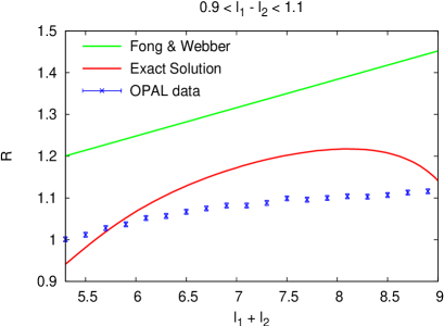
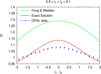
Figure 2: Two-particle correlations in two quark jets $\left(R=\frac{1}{2}+\frac{1}{2}{\cal C}^{(2)}_{Q}\right)$ [5] in the process $e^{+}e^{-}\to q\bar{q}$ as a function of $\ell_{1}+\ell_{2}=|\ln(x_{1}x_{2})|$ for $\ell_{1}-\ell_{2}=\ln(x_{2}/x_{1})=1.0$ (left) and $\ell_{1}-\ell_{2}=|\ln(x_{2}/x_{1})|$ for $\ell_{1}+\ell_{2}=\ln(x_{1}x_{2})=6.0$ (right).

Consequently, as displayed in Fig.2, the normalization of the more accurate solution of the evolution equations is lower and reproduces some features of the OPAL data at the $Z^{0}$ peak $Q=91.2$ GeV of the $e^{+}e^{-}$ annihilation, like the flattening of the slopes towards smaller values of $x$ [5]. Qualitatively, our MLLA expectations agree better with available OPAL data than the Fong–Webber predictions [5]. There remains however a significant discrepancy, markedly at very small $x$. In this region nonperturbative effects are likely to be more pronounced. They may undermine the applicability to particle correlations of the LPHD considerations that were successful in translating parton level predictions to hadronic observations in the case of more inclusive single particle energy spectra [1].

These measurements were redone by the CDF Collaboration for $p\bar{p}$ collisions at center of mass energy $\sqrt{s}=1.96$ TeV for mixed samples of quark and gluon jets [7]. For comparison with CDF data, the two-particle correlator was normalized by the corresponding multiplicity correlator of the second rank, which defines the dispersion of the mean average multiplicity inside the jet. In this case, the MLLA solution by Fong and Webber [4], the more accurate MLLA solution [5], and the NMLLA solution [3] were compared with the CDF data. The Fong-Webber predictions turned out to be in good agreement with CDF data in a range from large to small $x$, also covering the region of the phase space where MLLA predictions should normally not be reliable, that is, for $x>0.1$ (see Fig.3). As these figures were taken from [7], different notations have been used in this case, for instance, $\ell\equiv\xi=\ln(1/x)$, $\Delta\xi=\xi-\xi_{max}$ ($\xi_{max}\equiv\ell_{max}=\frac{1}{2}\ln(Q/Q_{0})$) such that $\Delta\xi_{1}+\Delta\xi_{2}=\ell_{1}+\ell_{2}-\ln(Q/Q_{0})$ and $\Delta\xi_{1}-\Delta\xi_{2}=\ell_{1}-\ell_{2}$.

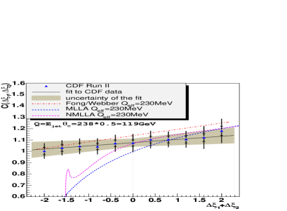
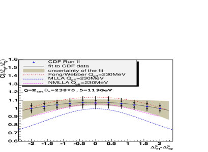
Figure 3: Two-particle correlations in a mixed sample of gluon and quark jets in $p\bar{p}$ collisions as a function of $\Delta\xi_{1}+\Delta\xi_{2}=|\ln(x_{1}x_{2})|-\ln(Q/Q_{0})$ for $\Delta\xi_{1}=\Delta\xi_{2}$ (left) and $\Delta\xi_{1}-\Delta\xi_{2}=|\ln(x_{2}/x_{1})|$ for $\Delta\xi_{1}=-\Delta\xi_{2}$ (right).

As observed in Fig.3 (left), the data are well described by the three cases in the interval $\Delta\xi_{1}+\Delta\xi_{2}>-0.5$, that is, at very small $x$. However, the Fong and Webber’s solution also describes the data for $\Delta\xi_{1}+\Delta\xi_{2}<-0.5$, that is, for larger values of $x$ where the MLLA is no longer valid. QCD color coherence for Fig.3 (left, the peak at $\Delta\xi_{1}+\Delta\xi_{2}=-1.5$ is due to numerical uncertainties) should be observed if the analysis is extended to $\Delta\xi_{1}+\Delta\xi_{2}>2.5$. Moreover, the NMLLA solution [3] extends, like for the $k_{\perp}$ spectra, the region of applicability of such predictions for larger values of $x$. In [7], it was concluded that despite the disagreement with the OPAL data in Fig.2, the LPHD stays successful for the description of less inclusive energy-momentum correlations. Therefore, in this paper we encourage the analysis of these observables by other collaborations like ALICE, ATLAS, and CMS in order to clarify this mismatch.

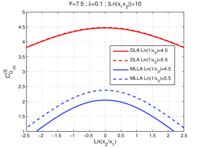
Figure 4: Gluon jet 3-particle correlator as a function of $|\ln(x_{1}x_{2})|$ for $x_{1}=x_{2}$ and $\ln(1/x_{3})$ (left) and as a function of $\ln(x_{2}/x_{1})$ for fixed $|\ln(x_{1}x_{2})|$ and $\ln(1/x_{3})$ (right).

3 Predictions for three-particle correlations and phenomenology

Finally, in order to extend the applicability of the LPHD to a larger domain of observables, we perform theoretical predictions for three-particle correlations in the limiting spectrum approximation ($Q_{0}\approx\Lambda_{QCD}$). This observable and two-particle correlations can be measured on equal footing at the LHC. We display the MLLA solutions (4) of the evolution equations (2) and (2). The correlators are functions of the variables $\ell_{i}$, $y_{i}$ and the virtuality of the jet $Q=E\Theta_{0}$. After setting $y_{i}=Y-\ell_{i}$ with fixed $Y=\ln(Q/Q_{0})$ in the arguments of the solutions (4), the dependence can be reduced to the following: ${\cal C}^{(3)}_{G_{123}}(\ell_{1},\ell_{2},\ell_{3},Y)$ and ${\cal C}^{(3)}_{Q_{123}}(\ell_{1},\ell_{2},\ell_{3},Y)$.

In Fig. 4, the DLA (2.1) and MLLA (4) three-particle correlators for $A=G$ and $A=Q,\bar{Q}$,

$${\cal C}^{(3)}_{G_{123}}=\frac{G^{(3)}_{123}}{G_{1}G_{2}G_{3}},\quad{\cal C}^{(3)}_{Q_{123}}=\frac{Q^{(3)}_{123}}{Q_{1}Q_{2}Q_{3}}$$

are displayed, respectively, as a function of the difference $(\ell_{1}-\ell_{2})=\ln(x_{2}/x_{1})$ for two fixed values of $\ell_{3}=\ln(1/x_{3})=4.5,\,5.5$, fixed sum $(\ell_{1}+\ell_{2})=|\ln(x_{1}x_{2})|=10$, and, finally, fixed $Y=7.5$ (virtuality $Q=450$ GeV and $\Lambda_{QCD}=250$ MeV), which is realistic for LHC phenomenology [5]. The representative values $\ell_{3}=\ln(1/x_{3})=4.5,\,5.5$ ($x_{3}=0.011,\,x_{3}=0.004$) have been chosen according to the range of the energy fraction $x_{i}\ll 0.1$, where the MLLA scheme can only be applied.

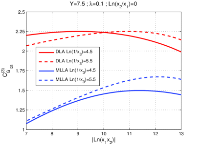
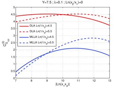
Figure 5: Quark jet 3-particle correlator as a function of $|\ln(x_{1}x_{2})|$ for $x_{1}=x_{2}$ and $\ln(1/x_{3})$ (left) and as a function of $\ln(x_{2}/x_{1})$ for fixed $|\ln(x_{1}x_{2})|$ and $\ln(1/x_{3})$ (right).

In Fig. 5, the DLA (2.1) and MLLA (4) three-particle correlators for $A=G$ and $A=Q,\bar{Q}$ are depicted, in this case as a function of the sum $(\ell_{1}+\ell_{2})=|\ln(x_{1}x_{2})|$ for the same values of $\ell_{3}=\ln(1/x_{3})=4.5,\,5.5$, for $x_{1}=x_{2}$ and $Y=7.5$. As expected in both cases, the DLA and MLLA three-particle correlators are larger inside a quark than in a gluon jet. Of course, these plots will be the same and the interpretation will apply to all possible permutations of three particles (123). As remarked above, the difference between the DLA and MLLA results is quite important in pointing out that overall corrections in ${\cal O}(\sqrt{\alpha_{s}})$ are large. Indeed, the last behavior is not surprising as it was already observed in the treatment of multiplicity fluctuations of the third kind given by $R_{3}=4.52\left[1-(2.280-0.018n_{f})\sqrt{\alpha_{s}}\right]$ [10].

For instance, for one quark jet produced at the $Z^{0}$ peak of the $e^{+}e^{-}$ annihilation ($Q=45.6$ GeV), one has $\alpha_{s}=0.134$. Replacing this value into the previous formula for the quark jet multiplicity correlator, one obtains a variation from 4.52 (DLA) to 0.83 (MLLA). Because of this, DLA has been known to provide unreliable predictions which should not be compared with experiments. From Fig.4, the correlation is observed to be the strongest when particles have the same energy and to decrease when one parton is harder than the others. Indeed, in this region of the phase space two competing constraints should be satisfied: as a consequence of gluon coherence and AO, gluon emission angles should decrease and on the other hand, the convergence of the perturbative series $k_{\perp}=x_{i}E\Theta_{i}\geq Q_{0}$ should be guaranteed. That is why, as the collinear cutoff parameter $Q_{0}$ is reached, gluons are emitted at larger angles and destructive interferences with previous emissions occur. This effect is clearly observed in Fig. 4; the steep fall of the distribution is more pronounced in the quark jet than in the gluon jet. Moreover, the observable increases for softer partons with $x_{3}$ decreasing, which is for partons less sensitive to the energy balance. In Fig.5 the MLLA correlations increase for softer partons, then flatten and decrease as a consequence of soft gluon coherence, reproducing for three-particle correlations the hump-backed shape of the one-particle distribution. Because of the limitation of phase space, one has ${\cal C}^{(3)}\leq 1$ for harder partons.

4 Summary

In this paper we provide the first full perturbative QCD treatment of three-particle correlations in parton showers, provide a further test of the LPHD within the limiting spectrum approximation, and briefly revise the comparison of two-particle correlations with OPAL and CDF data. The correlations have been shown to be strongest for the softest hadrons having the same energy $x_{1}=x_{2}=x_{3}$ in both quark and gluon jets, increasing as a function of $\ln(x_{i}/x_{j})$ and $|\ln(x_{i}x_{j})|$ when $x_{k}$ softens, that is for partons less sensitive to the energy balance. This result becomes therefore universal for $n$-particle correlations.

Coherence effects appear when one or two of the partons involved in the process are harder than the others, thus reproducing for this observable the hump-backed shape of the one-particle distribution. Also, the two- and three-particle correlations vanish (${\cal C}^{(2)}\to 1$) when one of the partons becomes very soft, thus describing the hump-backed shape of the one-particle distribution. The reason for that is dynamical rather than kinematical: radiation of a soft gluon occurs at large angles, which makes the radiation coherent and thus insensitive to the internal parton structure of the jet ensemble.

We give the first analytical predictions of this observable in view of forthcoming measurements by ATLAS, CMS, and ALICE at the LHC. Further information from the comparison with forthcoming data may also help to improve Monte Carlo event generators in the soft region of the phase space in intrajet cascades, where PYTHIA, ARIADNE and HERWIG face difficulties while reproducing the data [11].

We gratefully acknowledge enlightening discussions with W. Ochs and E. Sarkisyan-Grinbaum as well as support from Generalitat Valenciana under Grant No. PROMETEO/2008/004. M.A.S. acknowledges support from FPA2008-02878 and GVPROMETEO2010-056. V.M acklowledges support from the grant HadronPhysics2, a FP7-Integrating Activities and Infrastructure Program of the European Commission under Grant No. 227431, by UE (Feder), and by the MICINN (Spain) Grant No. FPA 2010-21750-C02-01.

References

• [1] Yu.L. Dokshitzer, V.A. Khoze, A.H. Mueller & S.I. Troyan, Basics of Perturbative QCD, Editions FrontiΓ¨res, Paris (1991).
• [2] Ya.I. Azimov, Yu.L. Dokshitzer, V.A. Khoze & S.I. Troian, Z. Phys. C 27 (1985) 65; Yu.L. Dokshitzer, V.A. Khoze & S.I. Troian, J. Phys. G 17 (1991) 1585.
• [3] Redamy PΓ©rezΒ Ramos, Francois Arleo, and Bruno Machet, Phys. Rev. D 78 (2008) 014019.
• [4] C.P. Fong, B.R. Webber, Nucl. Phys. B 355 (1991) 54;
ibid., Phys. Lett. B 241 (1990) 255.
• [5] R. PΓ©rez Ramos, JHEP 06 (2006) 019; R. PΓ©rez Ramos, JHEP 09 (2006) 014.
• [6] P.Β D. Acton etΒ al., Phys. Lett. B 287 (1992) 401.
• [7] T.Β Aaltonen etΒ al., Phys. Rev. D 77 (2008) 092001.
• [8] Yu.Β L. Dokshitzer, VictorΒ S. Fadin, and ValeryΒ A. Khoze, Z. Phys. C 18 (1983) 37.
• [9] Yu.L. Dokshitzer, Phys. Lett. B 305 (1993) 295.
• [10] E.D. Malaza & B.R. Webber, Phys. Lett. B 149 (1984) 501; E.D. Malaza & B.R. Webber, Nucl. Phys. B 267 (1986) 702.
• [11] G.Β Abbiendi etΒ al., Phys. Lett. B 638 (2006 ) 30.