Spin segregation via dynamically induced long-range interaction in a system of ultracold fermions

Abstract

We investigate theoretically the time evolution of a one-dimensional system of spin-1/2 fermions in a harmonic trap after, initially, a spiral spin configuration far-from equilibrium is created. We predict a spin segregation building up in time already for weak interaction under realistic experimental conditions. The effect relies on the interplay between exchange interaction and the harmonic trap, and it is found for a wide range of parameters. It can be understood as a consequence of an effective, dynamically induced long-range interaction that is derived by integrating out the rapid oscillatory dynamics in the trap.

I Introduction

Ultracold atomic quantum gases have been established as a clean and tunable test ground for many-body physics BlochEtAl08 . They allow to mimic condensed matter, but offer also opportunities to study aspects of many-body physics that are hard to address in other systems. An important example for the latter is the broad and widely unexplored subject of many-body dynamics. In this paper we investigate theoretically the spinor dynamics of a Fermi gas far away from equilibrium. We consider a one-dimensional system of repulsively interacting spin-1/2 fermions confined in a harmonic trap. The initial state is created out of the spin-polarized equilibrium by rotating the spins spatially into a spiral configuration (as previously done for a Bose condensate Vengalattore08 and proposed for strongly interacting fermions for the purpose of probing the Stoner transition ConduitAltman10 ). We show that already weak interaction, like in the experiment described in Refs. DuEtAl ; DuEtAlTheo , is sufficient to induce a robust spin segregation. The effect builds up on times that are long compared to the oscillatory motion of the atoms in the trap. It can be explained as a consequence of an effective, dynamically created long-range interaction that we obtain by integrating out the rapid oscillatory dynamics in the trap. Within the framework of a semiclassical theory, the effective interaction is isotropic in phase space. The fact that away from equilibrium already weak interaction can cause a noticeable spin segregation contrasts with the equilibrium physics of the system. For example, the spin segregation of itinerant ferromagnetism, possible signatures of which have recently been observed in a cold-atom system JoEtAl09 , requires strong interparticle repulsion as well as higher dimensions. The experiment JoEtAl09 has inspired also theoretical work on the dynamics of strongly-interacting spin-1/2 fermions, e.g. Refs. ConduitAltman10 ; dyn . In this paper we stick, however, to the regime of weak interaction, where the fermionic cold-atom system does not suffer from effects originating from the coupling to molecular two-body bound states such as dissipative particle losses PekkerEtAl11 or non-universal scattering properties ZhouEtAl11 .

In the following two sections we will first introduce the system and describe the semiclassical mean-field theory that we use to simulate its dynamics. In section IV we then present our numerical results, predicting a dynamical spin segregation. By integrating out rapid oscillations in the trap, in section V we derive an effective description for the dynamics that explains this finding in an intuitive fashion as a consequence of a dynamically induced long-range interaction. Before we close with conclusions, experimental signatures are discussed.

II System

We consider a gas of fermionic atoms of mass $M$ having two relevant internal states, $m=\frac{1}{2},-\frac{1}{2}\equiv\uparrow,\downarrow$. The gas is not necessarily quantum degenerate but sufficiently cold and dilute to interact via low-energy $s$-wave scattering only. Consequently, the interaction between two particles is captured by a pseudo potential $g^{\prime}P_{m_{1}^{\prime}m_{1},m_{2}^{\prime}m_{2}}\delta({\bm{r}}_{1}-{\bm{r}}_{2})$ with $(m_{1},m_{2})$ and $(m_{1}^{\prime},m_{2}^{\prime})$ denoting the spin state before and after scattering, respectively. Here

$$P_{m_{1}^{\prime}m_{1},m_{2}^{\prime}m_{2}} = \frac{1}{2}(e_{m_{1}^{\prime}m_{1}}e_{m_{2}^{\prime}m_{2}}-e_{m_{2}^{\prime}m_{1}}e_{m_{1}^{\prime}m_{2}})$$ (1)

$$= \frac{1}{4}e_{m_{1}^{\prime}m_{1}}e_{m_{2}^{\prime}m_{2}}-{\bm{s}}_{m_{1}^{\prime}m_{1}}\cdot{\bm{s}}_{m_{2}^{\prime}m_{2}}$$

with unity matrix $e_{m^{\prime}m}$ and vector of spin-1/2 matrices ${\bm{s}}_{m^{\prime}m}$, projects onto the antisymmetric spin singlet state two scattering particles have (due to Fermi statistics and the symmetric $s$-wave state). The term $-\frac{1}{2}e_{m_{2}^{\prime}m_{1}}e_{m_{1}^{\prime}m_{2}}=-\frac{1}{4}e_{m_{1}^{\prime}m_{1}}e_{m_{2}^{\prime}m_{2}}-{\bm{s}}_{m_{1}^{\prime}m_{1}}\cdot{\bm{s}}_{m_{2}^{\prime}m_{2}}$, corresponding to the so-called exchange interaction, gives rise to spin-spin coupling. The coupling constant $g^{\prime}=4\pi\hbar^{2}a_{s}/M$ is proportional to the singlet s-wave scattering length $a_{s}$, characterizing the actual interatomic potential. With this, we can write down the Hamiltonaian $\hat{H}^{\prime}=\int\!\mathrm{d}{\bm{r}}\,\hat{\psi}^{{\dagger}}_{m^{\prime}}({\bm{r}})h^{\prime}_{m^{\prime}m}({\bm{r}})\hat{\psi}_{m}({\bm{r}})+\frac{g^{\prime}}{2}\int\!\mathrm{d}{\bm{r}}\,\hat{\psi}^{{\dagger}}_{m_{1}^{\prime}}({\bm{r}})\hat{\psi}^{{\dagger}}_{m_{2}^{\prime}}({\bm{r}})P_{m_{1}^{\prime}m_{1},m_{2}^{\prime}m_{2}}\hat{\psi}_{m_{2}}({\bm{r}})\hat{\psi}_{m_{1}}({\bm{r}})$. Repeated spin indices imply summation, $\hat{\psi}_{m}({\bm{r}})$ is a fermionic field operator, and $h^{\prime}_{m^{\prime}m}({\bm{r}})=-\frac{\hbar^{2}}{2M}\nabla_{\bm{r}}^{2}e_{m^{\prime}m}+V_{m^{\prime}m}^{\prime}({\bm{r}})$ denotes the single-particle Hamiltonian containing the potential $V_{m^{\prime}m}^{\prime}({\bm{r}})=V({\bm{r}})e_{m^{\prime}m}+{\bm{B}}({\bm{r}})\cdot{\bm{s}}_{m^{\prime}m}$ that can be decomposed into a spin-independent term $V^{\prime}({\bm{r}})$ and an effective magnetic field ${\bm{B}}({\bm{r}})$ acting on the spin.

We are interested in the regime where the dynamics is reduced to one spatial dimension and consider a harmonic confining potential $V^{\prime}({\bm{r}})\equiv V(x)+V_{\perp}(y,z)=\frac{1}{2}M[\omega^{2}x^{2}+\omega_{\perp}^{2}(y^{2}+z^{2})]$ with the a tight transversal confinement $\omega_{\perp}$ being large compared to other relevant energy scales such as the initial temperature or chemical potential. Therefore, the particles basically occupy the transversal single-particle ground state. Moreover, we assume that the magnetic field varies in $x$-direction only, ${\bm{B}}({\bm{r}})=B_{0}{\bm{e}}_{z}+{\bm{B}}(x)$. A possibly present constant part $B_{0}{\bm{e}}_{z}$ of the magnetic field will be dropped in the following, i.e. we are working in a spin frame rotating around the $z$-axis. Introducing a dimensionless description in units of the longitudinal trap [energies, lengths, momenta, and times are given from now on in multiples of $\hbar\omega$, $(M\omega/\hbar)^{\!-1/2}$, $(M\hbar\omega)^{\!1/2}$, and $\omega^{-1}$, respectively] we arrive at the Hamiltonian

$$\hat{H} = \int\!\mathrm{d}x\,\hat{\psi}^{{\dagger}}_{m^{\prime}}(x)h_{m^{\prime}m}(x)\hat{\psi}_{m}(x)$$

$$+\frac{g}{2}\int\!\mathrm{d}x\,\hat{\psi}^{{\dagger}}_{m_{1}^{\prime}}(x)\hat{\psi}^{{\dagger}}_{m_{2}^{\prime}}(x)P_{m_{1}^{\prime}m_{1},m_{2}^{\prime}m_{2}}\hat{\psi}_{m_{2}}(x)\hat{\psi}_{m_{1}}(x)$$

for the one-dimensional problem. Here $g=2\hbar\omega_{\perp}a_{s}\times(M\omega/\hbar)^{\!1/2}/(\hbar\omega)$,

$$h_{m^{\prime}m}(x)=-\frac{1}{2}\partial^{2}_{x}e_{m^{\prime}m}+V_{m^{\prime}m}(x),$$ (3)

and

$$V_{m^{\prime}m}(x)=\frac{1}{2}x^{2}e_{m^{\prime}m}+{\bm{B}}(x)\cdot{\bm{s}}_{m^{\prime}m}.$$ (4)

By swapping field operators and indices ($\hat{\psi}^{{\dagger}}_{m_{1}^{\prime}}\hat{\psi}^{{\dagger}}_{m_{2}^{\prime}}=-\hat{\psi}^{{\dagger}}_{m_{2}^{\prime}}\hat{\psi}^{{\dagger}}_{m_{1}^{\prime}}\to-\hat{\psi}^{{\dagger}}_{m_{1}^{\prime}}\hat{\psi}^{{\dagger}}_{m_{2}^{\prime}}$) the interaction can be simplified to $\hat{H}_{\text{int}}=g\int\!\mathrm{d}x\,\hat{\psi}^{{\dagger}}_{\uparrow}(x)\hat{\psi}_{\uparrow}(x)\hat{\psi}^{{\dagger}}_{\downarrow}(x)\hat{\psi}_{\downarrow}(x)$ reflecting that by Pauli exclusion only fermions of opposite spin interact. The resulting spin coupling – parallel spins avoid repulsion – is expressed more clearly, however, in Eqs. (1) and (II).

III Semiclassical description

III.1 Equations of motion

We study the system’s dynamics in terms of the single-particle density matrix

$$n_{m^{\prime}m}(x^{\prime},x)\equiv\text{tr}\{\hat{\rho}\hat{\psi}^{{\dagger}}_{m^{\prime}}(x^{\prime})\hat{\psi}_{m}(x)\}$$ (5)

with density operator $\hat{\rho}$. It evolves in time according to $\mathrm{i}\dot{\hat{\rho}}=[\hat{H},\hat{\rho}]$, giving

$$\mathrm{i}\,\dot{n}_{m^{\prime}m}(x^{\prime},x)=\langle[\hat{\psi}^{{\dagger}}_{m^{\prime}}(x^{\prime})\hat{\psi}_{m}(x),\hat{H}]\rangle.$$ (6)

using cyclic permutation under the trace. While for non-interacting particles the r.h.s. of this equation reads $h_{mk}(x)n_{m^{\prime}k}(x^{\prime},x)-h_{km^{\prime}}(x)n_{km}(x^{\prime},x)$, the interaction $\hat{H}_{\text{int}}$ leads to quartic expectation values that we decompose like

$$\langle\hat{\psi}^{{\dagger}}_{k}\hat{\psi}^{{\dagger}}_{l}\hat{\psi}_{m}\hat{\psi}_{n}\rangle\approx\langle\hat{\psi}^{{\dagger}}_{k}\hat{\psi}_{n}\rangle\langle\hat{\psi}^{{\dagger}}_{l}\hat{\psi}_{m}\rangle-\langle\hat{\psi}^{{\dagger}}_{k}\hat{\psi}_{m}\rangle\langle\hat{\psi}^{{\dagger}}_{l}\hat{\psi}_{n}\rangle$$ (7)

in order to get a closed equation for $n_{m^{\prime}m}(x^{\prime},x)$. By Wick’s theorem this decomposition is exact for the initial state considered here, being an equilibrium state of a quadratic Hamiltonian modified only by the spiral spin rotation generated by another quadratic Hamiltonian. At later times it corresponds to the time-dependent Hartree-Fock approximation that is suitable for weak interaction and leads to the non-linear equation of motion

$$\mathrm{i}\dot{n}_{m^{\prime}m}(x^{\prime},x)=h^{\text{mf}}_{mk}(x)n_{m^{\prime}k}(x^{\prime},x)-h^{\text{mf}}_{km^{\prime}}(x^{\prime})n_{km}(x^{\prime},x).$$ (8)

The Hartree-Fock Hamiltonian $h^{\text{mf}}_{m^{\prime}m}(x)=h_{m^{\prime}m}(x)+V_{m^{\prime}m}^{\text{mf}}(x)$ comprises the mean-field potential $V^{\text{mf}}_{m^{\prime}m}(x)=V_{\text{mf}}(x)e_{m^{\prime}m}+{\bm{B}}_{\text{mf}}(x)\cdot{\bm{s}}_{m^{\prime}m}$ where

$$V_{\text{mf}}(x) = \frac{1}{2}gn_{0}(x),$$

$${\bm{B}}_{\text{mf}}(x) = -2g{\bm{n}}(x),$$ (9)

with particle density $n_{0}(x)=e_{m^{\prime}m}n_{m^{\prime}m}(x,x)$ and spin density ${\bm{n}}(x)={\bm{s}}_{m^{\prime}m}n_{m^{\prime}m}(x,x)$.

In a next step, we introduce the Wigner function

$$w_{m^{\prime}m}(x,p)=\frac{1}{2\pi}\int\!\mathrm{d}\xi\,\mathrm{e}^{-\mathrm{i}p\xi}n_{m^{\prime}m}(x-\xi/2,x+\xi/2).$$ (10)

Using Eq. (8), this phase-space representation of the single-particle density matrix can be shown to evolve like (e.g. Schleich )

$$\dot{w}_{m^{\prime}m}(x,p)=-p\partial_{x}w_{m^{\prime}m}(x,p)+\frac{1}{\mathrm{i}}\sum_{\alpha=0}^{\infty}\frac{1}{\alpha!}\Big{(}\frac{\mathrm{i}}{2}\partial_{y}\partial_{p}\Big{)}^{\!\alpha}$$

$$\times[\bar{V}_{mk}(y)w_{m^{\prime}k}(x,p)-(-)^{\alpha}\bar{V}_{km^{\prime}}(y)w_{km}(x,p)]\Big{|}_{y=x}$$ (11)

with $\bar{V}_{m^{\prime}m}(x)\equiv V_{m^{\prime}m}(x)+V_{m^{\prime}m}^{\text{mf}}(x)$. The relation

$$n_{m^{\prime}m}(x,x)=\int\!\mathrm{d}p\,w_{m^{\prime}m}(x,p)$$ (12)

connecting the spatial densities entering the mean-field potential to the Wigner function closes this equation of motion. We employ a semiclassical approximation to the motional degrees of freedom by truncating the infinite series after $\alpha=1$. This is justified as long as the potential $\bar{V}_{m^{\prime}m}(x)$ varies slowly compared to the single-particle wave lengths involved. It is, thus, particularly suitable for sufficiently hot or dense systems, with either the thermal or the Fermi wave length small. Moreover, the truncation is exact for harmonic or linear potentials $\bar{V}_{m^{\prime}m}(x)$. It gives

$$\dot{w}_{m^{\prime}m} = -p\partial_{x}w_{m^{\prime}m}+(\partial_{x}\bar{V})\partial_{p}w_{m^{\prime}m}$$ (13)

$$-\mathrm{i}\bar{\bm{B}}\cdot({\bm{s}}_{mk}w_{m^{\prime}k}-{\bm{s}}_{km^{\prime}}w_{km})$$

$$+\frac{1}{2}(\partial_{x}\bar{\bm{B}})\cdot\partial_{p}({\bm{s}}_{mk}w_{m^{\prime}k}+{\bm{s}}_{km^{\prime}}w_{km})$$

having the form of a Boltzmann equation, lacking the collision integral and augmented by a coherent spin-dynamics, cf., e.g., FuchsEtAl08 and references therein. On the r.h.s., the four terms describe diffusion, spin-independent acceleration, coherent spin rotation, and spin-dependent acceleration, respectively. It is instructive to introduce the real-valued density and spin Wigner functions

$$w_{0}(x,p) \equiv e_{m^{\prime}m}w_{m^{\prime}m}(x,p),$$

$${\bm{w}}(x,p) \equiv {\bm{s}}_{m^{\prime}m}w_{m^{\prime}m}(x,p).$$ (14)

Their time evolution is determined by (e.g. Ref. FuchsEtAl08 )

$${\dot{w}}_{0} = \big{(}-p\partial_{x}+x\partial_{p}+(\partial_{x}V_{\text{mf}})\partial_{p}\big{)}w_{0}$$

$$+\,\big{(}\partial_{x}{\bm{B}}+\partial_{x}{\bm{B}}_{\text{mf}}\big{)}\cdot\partial_{p}{\bm{w}},$$

$${\dot{\bm{w}}} = \big{(}-p\partial_{x}+x\partial_{p}+(\partial_{x}V_{\text{mf}})\partial_{p}+({\bm{B}}+{\bm{B}}_{\text{mf}})\times\big{)}{\bm{w}}$$ (15)

$$+\,\frac{1}{4}\big{(}\partial_{x}{\bm{B}}+\partial_{x}{\bm{B}}_{\text{mf}}\big{)}\partial_{p}w_{0},$$

where ${\bm{B}}\neq 0$ only during the preparation while during the time evolution to be simulated ${\bm{B}}=0$.

The quantum and fermionic nature of the system enters into the equations of motion (III.1) in different ways: through the initial state $(w_{0},{\bm{w}})$, via the coherent spin dynamics, and with the structure of the mean-field interaction (III.1) stemming from the projection on spin-singlet scattering (1) for Fermi-statistics. Equations (III.1) describe the collisionless regime of weak interaction (implicitely assumed when introducing the mean-field approximation FuchsEtAl08 ). The collisionless regime is opposed to the hydrodynamic regime where collisions constantly restore a local equilibrium of the momentum distribution such that the state is described by density and velocity fields depending on $x$ only. Both regimes can be found in the very same system: The one-dimensional collisionless description by the set of equations (III.1) is also valid when the transversal confinement $\omega_{\perp}$ is not tight enough to freeze out transversal motion completely (as assumed here), but still tight enough to ensure quick equilibration along the transversal directions instead DuEtAl ; DuEtAlTheo . The results presented in this paper are, therefore, also valid in this quasi-one-dimensional regime. The regime in between the collisionless and hydrodynamic limit is captured by adding a collision integral to Eqs. (III.1) tending to restore thermal equilibrium on a scale $\tau_{\text{coll}}$. Considering the effect of collisions along the longitudinal direction $x$ becomes necessary when considering stronger interactions and longer times scales as we do. For such a regime, it has been proposed to observe the spin-wave instability predicted by Castaing in a quantum gas FuchsEtAl02 .

III.2 Initial off-equilibrium state

Initially, the system is prepared in its spin-polarized equilibrium state, with the spins pointing in $x$-direction, temperature $T$, and chemical potential $\mu$. One has

$$w_{0}(x,p)=\frac{1}{2\pi}\Big{\{}\exp\Big{[}\frac{1}{T}\Big{(}\frac{1}{2}p^{2}+\frac{1}{2}x^{2}-\mu\Big{)}\Big{]}+1\Big{\}}^{-1}$$ (16)

and ${\bm{w}}=(1,0,0)^{\text{t}}w_{0}/2$ (with), or $w_{m^{\prime}m}=w_{0}/2$. The zero-temperature chemical potential, the Fermi energy for just one spin-state, simply reads $E_{F}=N$ with total particle number $N=\int\!\mathrm{d}x\,n_{0}(x)=\int\!\mathrm{d}x\!\int\!\mathrm{d}p\,w_{0}(x,p)$. This description of the initial state is accurate, since the spin-polarized gas is non-interacting and the semiclassical approximation exact for a harmonic trap. In a next step, at time $t=0$, during a short preparatory pulse a $z$-polarized magnetic field gradient is applied, captured by ${\bm{B}}(x)=qx\delta(t){\bm{e}_{z}}$. A spin spiral of wave length $\lambda_{s}=2\pi/q$ is created, while $w_{0}(x,p)$ is still given by Eq. (16) one has

$${\bm{w}}(x,p)=\big{(}\cos(qx),\sin(qx),0\big{)}^{\text{\!t}}\,\frac{w_{0}(x,p)}{2}.$$ (17)

or $w_{m^{\prime}m}(x,p)=\exp[\mathrm{i}qx(m-m^{\prime})]w_{0}(x,p)/2$. With a simple spin rotation, we have prepared a state far from thermal equilibrium. Apart from (i) having created a rather artificial spiral spin configuration (17) (favorable neither with respect to energy nor entropy), we have also increased the number of available single-particle states from one spin state to two. The latter has two consequences: (ii) the phase-space density configuration (16) is far from being thermal (for half the number of particles per spin state having the same kinetic energy as before, a thermal distribution is characterized by a lower chemical potential and a higher temperature), and (iii) we have suddenly introduced interaction to the system. The combination of (i) and (iii) will lead to robust dynamical spin segregation.

III.3 Semiclassical versus mean-field dynamics

When integrating the time evolution for many fermions, the semiclassical phase-space equations (III.1) are usually much easier to treat numerically than the Hartree-Fock mean-field equations. (8), even though the interaction is non-local in the former,

$$V_{\text{mf}}(x) = \frac{g}{2}\int\!\mathrm{d}p\,w_{0}(x,p),\quad$$

$${\bm{B}}_{\text{mf}}(x) = -2g\int\!\mathrm{d}p\,{\bm{w}}(x,p).$$ (18)

This is exemplified by our state (16) and (17): In phase space, it has a linear extent $\Delta\sim\sqrt{\max(\mu,T)}$ [we define $\Delta\equiv 2\max(\sqrt{2N},2\sqrt{T})$], while it varies on the scale $\delta\sim\min\big{(}T/\Delta,\lambda_{s}\big{)}$ stemming either from the former equilibrium [roughly estimating $\frac{\mathrm{d}w_{0}}{\mathrm{d}\varepsilon}\frac{\mathrm{d}\varepsilon}{\mathrm{d}s}\sim\frac{w_{0}}{T}\Delta$ with $\varepsilon=\frac{1}{2}(x^{2}+p^{2})$ and $s=x,p$] or from the induced spin spiral. For a reasonable phase-space representation one, thus, requires a grid of just more than $(\Delta/\delta)^{2}\sim N$ points. On the other hand, the real-space single-particle density matrix $n_{m^{\prime}m}(x^{\prime},x)$ varies on the much shorter length $\delta^{\prime}\sim\Delta^{-1}$ in each argument, calling for more than $\Delta^{4}\gtrsim N^{2}$ grid points.

IV Simulation of dynamics

IV.1 System parameters

In the following we consider Li⁶ atoms with mass $M\approx 1.0\cdot 10^{-26}$ kg and the scattering length tuned down to $a_{s}\approx 2.4\cdot 10^{-10}{\rm m}$ by using a magnetic Feshbach resonance; the trap frequencies read $\omega=2\pi\cdot 60$ Hz and $\omega_{\perp}=2\pi\cdot 3.6$ kHz. Returning to dimensionless units, we obtain the weak coupling $g\approx 0.055$. The initial spin-polarized equilibrium is characterized by the particle number $N=E_{F}=100$ and by the temperature $T$ taking values of either $T/E_{F}=$ 0.2, 1, or 5 corresponding to the degenerate, intermediate and non-degenerate regime. According to these values one finds: the chemical potentials $\mu/E_{F}\approx$ 1.0, 0.54, -7.2; cloud extensions $\Delta\approx$ 28, 40, 89; maximum densities $n_{0}(0)\approx$ 4.4, 3.3, 1.8; and maximum mean-field potential strengths $n_{0}(0)g\approx$ 0.24, 0.18, 0.097 that are small compared to the trap frequency, being 1 in our units, and extremely small with respect to typical single-particle energies $\max(T,\mu)\gtrsim 100$. In addition to the temperature, we also vary the spiral wave length $\lambda_{s}$ and consider either $\Delta/\lambda_{s}=$ 1, 2 or 5 windings of the spin spiral within the atom cloud. For these conditions, we integrate the time evolution using a MacCormack method MacCormack03 and trust results that coincide for grid-sizes $300^{2}$ and $600^{2}$ for a phase space region of linear extension $\approx 2\Delta$.

IV.2 Observation of spin segregation

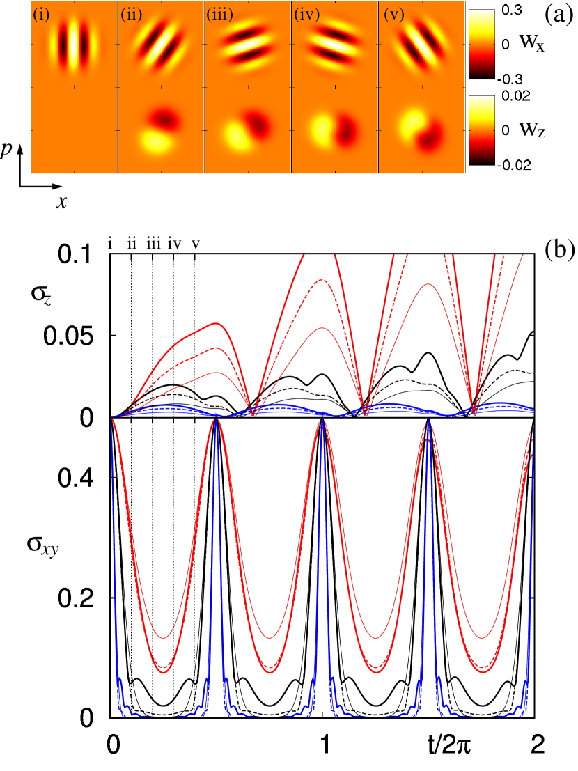
Figure 1: (Color online) (a) Wigner functions $w_{x}(x,p)$ and $w_{z}(x,p)$ at five times [i-v, as indicated in (b)] during the first half cycle; $T/E_{F}=1$, $\lambda_{s}/\Delta=0.5$, both $x$ and $p$ range from -40 to 40. The motion in phase space is governed by an overall rotation at the trap frequency, during which the $z$-component of the Wigner function slowly builds up two domains. (b) Time evolution of the averaged spatial polarizations $\sigma_{z}$ and $\sigma_{xy}$ for $T/E_{F}=$ 0.2, 1, 5 (thick solid, dashed, and thin solid lines, respectively) and for $\lambda_{s}/\Delta=$ 1, 0.5, 0.2 (upper triple of red, central triple of black, and lower triple of blue lines, respectively). While for the shorter wave lengths $\lambda_{s}/\Delta$ the spatial $xy$-polarization shows rapid collapses followed by periodic revivals, the emerging spatial $z$-polarization undergoes smooth oscillations as a signature of the formation of only two domains in phase space.

On a short time scale $\sim 1$, the system evolves mainly as determined by the harmonic trapping potential. That is, neglecting interaction completely for the moment, $\big{(}w_{0}(x,p),{\bm{w}}(x,p)\big{)}$ simply rotates in phase space at constant angular velocity 1 (in units of the trap); each point of the Wigner function follows a classical circular orbit. This behavior can be observed clearly in the first row of Fig. 1(a) showing the evolution of $w_{x}$ during half a cycle. This simple dynamics in phase space translates into a more involved evolution of the spatial polarization ${\bm{n}}(x)$, obtained by projecting ${\bm{w}}(x,p)$ onto the $x$-axis, ${\bm{n}}(x)=\int\!\mathrm{d}p\,{\bm{w}}(x,p)$. Fig. 1(b) shows the averaged absolute spatial $xy$-polarization,

$$\sigma_{xy}\equiv\frac{1}{N}\int\!\mathrm{d}x\,[n_{x}^{2}(x)+n_{y}^{2}(x)]^{\!1/2},$$ (19)

during the first two cycles. A rapid collapse of $\sigma_{xy}$ followed by periodic revivals can be observed, the more pronounced the larger the number of spiral windings $\Delta/\lambda_{s}$ in the atom cloud.

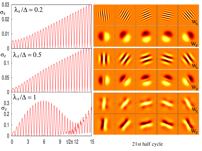
Figure 2: (Color online) Evolution on longer times, for $T/E_{F}=1$, and different wave lenghts $\lambda_{s}/\Delta$. The l.h.s. shows the averaged spatial absolute $z$-polarization, $\sigma_{z}$, versus time. On the r.h.s. the Wigner functions $w_{x}$ and $w_{z}$ are plotted for five instants of times like in Fig. 1(a), but during the 21st half cycle (arbitry color scale). Initially $\sigma_{z}$ increases linearly in time with a rate that is controlled by the wave length $\lambda_{s}/\Delta$. Irrespective of the number of windings $\Delta/\lambda_{s}$ (directly visible in $w_{x}$), $w_{z}$ developeds two oppositely polarized domains.

During a single cycle of oscillation in the trap the weak interaction causes only small deviations from a simple rotation in phase space. The small modification of the trap frequency and the slight anharmonicities caused by the scalar part of the mean-field potential $V_{\text{mf}}(x)$ are hardly noticeable. However, the effect of interaction becomes apparent in $w_{z}$, being zero initially [Fig. 1(a), note the different color scales for $w_{x}$ and $w_{z}$]. Though still small, $w_{z}$ develops a characteristic pattern induced by the magnetic mean field ${\bm{B}}_{\text{mf}}$. Namely, in $w_{z}$ two domains of opposite $z$-polarization form. This spin segregation in phase space corresponds to phase-opposed dipole oscillations of the $\uparrow$- and the $\downarrow$-polarized domain in the trap (see also Fig. 3). Remarkably, the spin segregation does not reproduce the structure of the initially created spin spiral of wave length $\lambda_{s}$. The formation of two spin domains (and only two) is a very robust effect; we find it for all pitches of the spin spiral considered here. The upper panel of Fig 1(b) shows the averaged absolute spatial $z$-polarization

$$\sigma_{z}\equiv\frac{1}{N}\int\!\mathrm{d}x\,[n_{z}^{2}(x)]^{\!1/2}.$$ (20)

As a consequence of spin segregation in phase space, $\sigma_{z}$ oscillates in time, however, because only two domains are formed, it does not feature sharp collapses like $\sigma_{xy}$ does for small $\lambda_{s}/\Delta$.

In Fig 2 we present data for longer times, for the original temperature $T/E_{F}=1$ and for three different spiral wave lengths $\lambda_{s}/\Delta$: From cycle to cycle the spin segregation becomes more and more pronounced as visible from $\sigma_{z}$ and from the snapshots on the r.h.s. showing $w_{z}$ during the 21st half cycle. The rotation in phase space of the two oppositely polarized domains corresponds to phase-opposed dipole oscillation of $\uparrow$ and $\downarrow$ spins in the trap. This behavior is visible in Fig. 3 showing the spatial densities $n_{\uparrow}(x)$ and $n_{\downarrow}(x)$ as well as the spatial polarization $n_{z}(x)=\frac{1}{2}[n_{\uparrow}(x)-n_{\downarrow}(x)]$ during the 21st cycle. While a $z$-polarization builds up, the spiral spin structure in the $xy$-plane decreases but stays intact (cf. $w_{x}$ during the 21st half cycle shown in Fig. 2). The total density Wigner function $w_{0}$ hardly changes during the time-evolution also for longer times (not shown). The spin segregation can directly be controlled by the number of windings $\Delta/\lambda_{s}$ of the spin spiral within the cloud, the more windings the slower the segregation builds up. The fastest segregation is observed for $\Delta/\lambda_{s}=1$, here already after 10 half cycles deviations from a linear increase is found and a more complex dynamics sets in (Fig. 2).

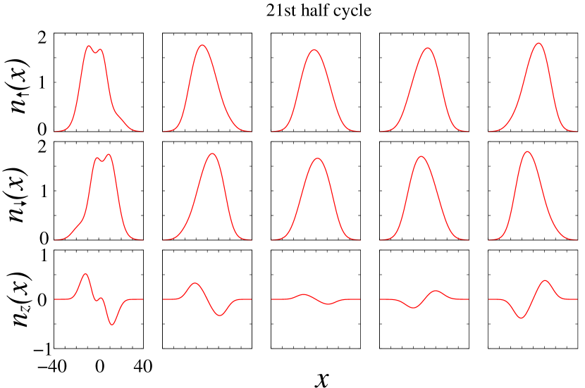
Figure 3: (Color online) Spatial densities $n_{\uparrow}(x)$ and $n_{\downarrow}(x)$ as well as $z$-polarization $n_{z}(x)=\frac{1}{2}[n_{\uparrow}(x)-n_{\downarrow}(x)]$ at five instants of time during the 21st half cycle, for $T/E_{F}=1$ and $\lambda_{s}/\Delta=0.2$. Times and parameters correspond to the middle row of the r.h.s. of Fig. 2. Spin $\uparrow$ and $\downarrow$ particles segregate and perform phase-opposed dipole oscillations in the trap.

V Explanation by dynamically induced long-range interaction

V.1 Effective Description

In order to give an intuitive explanation for the spin segregation, let us describe the system in the rotating phase-space frame with the new coordinates $x^{\prime}=x\cos(t)-p\sin(t)$ and $p^{\prime}=p\cos(t)+x\sin(t)$ describing classical orbits in the trap. In that frame ${\bm{w}}^{\prime}(x^{\prime},p^{\prime},t)\equiv{\bm{w}}(x(x^{\prime},p^{\prime},t),p(x^{\prime},p^{\prime},t),t)$ is stationary for vanishing interaction. However, interaction, represented by the mean-field potentials (III.3), is now time-dependent, since it is obtaned by projecting onto the $x$-axis that rotates with respect to the new frame. For example, the magnetic mean field ${\bm{B}}_{\text{mf}}^{\prime}(x^{\prime},p^{\prime},t)={\bm{B}}_{\text{mf}}(x(x^{\prime},p^{\prime},t),t)$ reads

$${\bm{B}}_{\text{mf}}^{\prime}(x^{\prime},p^{\prime},t)=-2g\int_{-\infty}^{\infty}\!\mathrm{d}s\,{\bm{w}}^{\prime}\big{(}x^{\prime}-s\sin(t),p^{\prime}+s\cos(t),t\big{)}.$$ (21)

The time-dependence of the mean field ${\bm{B}}_{\text{mf}}^{\prime}$ originates on the one hand from the rotation of the integration axis at trap frequency and on the other hand from the time-dependence of the Wigner function ${\bm{w}}^{\prime}(x^{\prime},p^{\prime},t)$. In the rotating frame, the latter is solely governed by the weak interaction and slow compared to the oscillation in the trap. We can use this difference in time scales to separate the dynamics on short times from that on longer times. We assume that a single oscillation in the trap is not affected by the weak interaction. This allows us, in turn, to integrate out the rapid oscillations in the trap when studying the dynamics on longer times where interaction does play a role; we approximate

$${\bm{B}}_{\text{mf}}^{\prime}(x^{\prime},p^{\prime},t)\approx{\bm{B}}^{\text{eff}}_{\text{mf}}(x^{\prime},p^{\prime},t)$$ (22)

$$\equiv\frac{-2g}{2\pi}\int_{0}^{2\pi}\!\mathrm{d}\tau\int_{-\infty}^{\infty}\!\mathrm{d}s\,{\bm{w}}^{\prime}\big{(}x^{\prime}-s\sin(\tau),p^{\prime}+s\cos(\tau),t\big{)}$$

giving

$${\bm{B}}^{\text{eff}}_{\text{mf}}(x^{\prime},p^{\prime},t)=\int\!\mathrm{d}\tilde{p}\int\!\mathrm{d}\tilde{x}\frac{-2g/\pi}{\sqrt{\tilde{x}^{2}+\tilde{p}^{2}}}{\bm{w}}^{\prime}\big{(}x^{\prime}+\tilde{x},p^{\prime}+\tilde{p},t\big{)}.$$ (23)

By averaging over a cycle, we have obtained an effective mean-field potential that corresponds to a time-independent isotropically long-ranged interaction in phase space. By oscillating in the trap, the system dynamically acquires a spatially long-range interaction.

V.2 Zero-order semiclassical mean-field interaction

We can simplify the description further, again arguing that interaction is weak and the mean-field potential small compared to the trap. For the mean-field contribution $V^{\text{mf}}_{m^{\prime}m}$ of the potential $\bar{V}_{m^{\prime}m}(x)=V^{\text{mf}}_{m^{\prime}m}(x)+\frac{1}{2}x^{2}$, appearing in the infinite series on the r.h.s. of the equation of motion (III.1), we truncate the series already after $\alpha=0$ instead of $\alpha=1$. In the set of equations (III.1), this approximation corresponds to neglecting the mean-field-induced acceleration by dropping terms involving the gradients $\partial_{x}{\bm{B}}_{\text{mf}}$ and $\partial_{x}V_{\text{mf}}$. We keep, however, the spin-rotating term ${\bm{B}}_{\text{mf}}\times{\bm{w}}$ stemming from the order $\alpha=0$. Together with cycle averaging, in the rotating phase-space frame, we arrive at the effective equations of motion

$$\dot{w}_{0}^{\prime}(x^{\prime},p^{\prime},t) = 0$$

$$\dot{\bm{w}}^{\prime}(x^{\prime},p^{\prime},t) = {\bm{B}}^{\text{eff}}_{\text{mf}}(x^{\prime},p^{\prime},t)\times{\bm{w}}^{\prime}(x^{\prime},p^{\prime},t).$$ (24)

The second equation describes the time evolution of the polarization field ${\bm{w}}^{\prime}$ in the $x^{\prime}p^{\prime}$-plane. At each point the polarization rotates in the mean field ${\bm{B}}^{\text{eff}}_{\text{mf}}$ such that $|{\bm{w}}^{\prime}|$ stays constant.

V.3 Growth of $z$-polarization

The spin segregation observed numerically can now be explained by first-order time-dependent perturbation theory, predicting according to Eqs. (V.2) initially a linear growth of the z-polarization,

$$w_{z}(x^{\prime},p^{\prime},t)\simeq[{\bm{B}}^{\text{eff}}_{\text{mf}}(x^{\prime},p^{\prime},0)\times{\bm{w}}^{\prime}(x^{\prime},p^{\prime},0)]_{z}t,$$ (25)

as we can observe it on the l.h.s. of Fig. 2. Deviations from the linear growth (25) appear as soon as $w_{z}^{\prime}$ becomes comparable to $|{\bm{w}}^{\prime}|$ as visible in the lower left plot of Fig. 2. Figure 4 shows the rate $[{\bm{B}}^{\text{eff}}_{\text{mf}}(0)\times{\bm{w}}^{\prime}(0)]_{z}$ computed for the intermediate temperature $T/E_{F}=1$ and different spiral wave lengths $\lambda_{s}/\Delta$. Notably $[{\bm{B}}^{\text{eff}}_{\text{mf}}(0)\times{\bm{w}}^{\prime}(0)]_{z}$ always shows a pattern with two oppositely polarized domains, irrespective of the number of windings $\Delta/\lambda_{s}$ . This explains the previously observed segregation of $\uparrow$ and $\downarrow$ polarization. The formation of two domains only can be understood as follows:

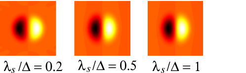
Figure 4: (Color online) Cycle-averaged rate of the creation of $z$-polarization computed for the initial state, $[{\bm{B}}^{\text{eff}}_{\text{mf}}(0)\times{\bm{w}}^{\prime}(0)]_{z}$, for $T/E_{F}=1$ and different spiral wave lenghts $\lambda_{s}/\Delta$ (arbitrary color scale). It explains the formation of two oppositely polarized domains in $w_{z}$ that is visible in Fig. 2.

According to Eq. (23), the spin polarization ${\bm{w}}^{\prime}$ at a given point $(x^{\prime},p^{\prime})$ in phase space feels a magnetic mean field that mainly depends on the polarization found in phase-space areas close by. Within the phase-space neighborhood of $(x^{\prime},p^{\prime})$, in turn, phase-space areas showing the largest polarization perpendicular to ${\bm{w}}^{\prime}(x^{\prime},p^{\prime})$ contribute most. Since for the initial state $|{\bm{w}}^{\prime}|=w_{0}^{\prime}/2$ increases towards the origin $x^{\prime}=p^{\prime}=0$, at a given point $(x^{\prime},p^{\prime})$ the effective magnetic mean field ${\bm{B}}^{\text{eff}}_{\text{mf}}$ is dominated by the polarization found when slightly moving along the direction of the spiral towards the origin. On one side of the spiral this results always in the creation of a positive $z$-polarization, on the other side always to the creation of a negative $z$-polarization. This explains the creation of two domains. Moreover, the strength of the local mean field depends on the spatial variation of the spin density $|{\bm{w}}^{\prime}|$ compared to the spiral wave length $\lambda_{s}$; the smaller $\lambda_{s}/\Delta$ the slower the spin segregation, as observed numerically in Fig. (2).

We have identified the mechanism underlying the observed spin segregation. Obviously, the phenomenon does not depend on the sign of the spin-spin coupling. We have checked numerically that it is equally observable for attractive interaction, giving reversed polarizations. Moreover, it can also be expected for non-condensed “spin-1/2” bosons which are equally described by Eqs. (III.1), but with the exchange interaction giving rise to a spin-coupling of opposite sign.

VI Experimental signatures

One can measure the dynamical spin segregation by state-sensitive absorption imaging either in situ (as in the experiment by Du et al. DuEtAl ) or after a time of flight. In the latter case one can also use Stern-Gerlach separation to distinguish $\uparrow$ and $\downarrow$ particles. An in situ measurement gives the spatial distributions $n_{m}(x)=\int\!\mathrm{d}p\,w_{mm}(x,p)$ of both spin states $m=\uparrow,\downarrow$; the images after a time of flight reveal their momentum distribution $\tilde{n}_{m}(p)=\int\!\mathrm{d}x\,w_{mm}(x,p)$. One can then determine the $z$-polarization in space, $n_{z}(x)=\frac{1}{2}[n_{\uparrow}(x)-n_{\downarrow}(x)]$, and momentum, $\tilde{n}_{z}(p)=\frac{1}{2}[\tilde{n}_{\uparrow}(p)-\tilde{n}_{\downarrow}(p)]$. As shown in Fig. 3, the dynamical spin segregation corresponds to phase-opposed dipole oscillations of $\uparrow$ and $\downarrow$ spins in space. The momentum distributions will show the very same behavior, but shifted in time by the quarter of a cycle (because momentum densities are obtained by projecting the Wigner function onto the $p$-axis).

VII Conclusions

The phenomenon of dynamical spin segregation predicted here is different from the effect observed by Du et al. described in Refs. DuEtAl ; DuEtAlTheo . In their case no spin spiral is created initially, instead an inhomogeneous external magnetic field is present throughout, leading eventually to a spherical symmetric spin segregation in phase space between an inner core and an outer shell. The phenomenon described here also differs from the physics of the spin-wave instability investigated by Conduit and Altman ConduitAltman10 . They consider the same spiral spin structure as initial state, but strong repulsive interaction. In contrast to the dynamical spin segregation into two counter oscillating domains found here, crucially depending on the presence of the trap, their spin-wave instability leads to spatial (non oscillatory) domain formation, not requiring a trap and with the domain size controlled by the spiral wave length.

The system’s dynamics described here can be called self driven. The transformation to the co-rotating frame in phase space corresponds to the transformation to the Dirac picture on the full quantum many-body level, where the quadratic Hamiltonian $\hat{H}_{0}=\hat{H}-\hat{H}_{\text{int}}$ constitutes the unperturbed problem. In the Dirac picture, the time evolution is generated solely by the time-dependent interaction Hamiltonian $\hat{H}^{\text{d}}_{\text{int}}(t)=\exp(-\mathrm{i}\hat{H}_{0}t/\hbar)\hat{H}_{\text{int}}\exp(\mathrm{i}\hat{H}_{0}t/\hbar)$. Thanks to the equidistant ladder spectrum of the harmonic trap, it is time periodic, $\hat{H}^{\text{d}}_{\text{int}}(t+\mathcal{T})=\hat{H}^{\text{d}}_{\text{int}}(t)$ with $\mathcal{T}=2\pi/\omega$, like the Hamiltonian of a driven system. This additional symmetry has strong consequences for the dynamics. It allows us to find a time-independent effective description $\hat{H}_{\text{eff}}=\frac{1}{\mathcal{T}}\int_{0}^{\mathcal{T}}\!\mathrm{d}t\,\hat{H}^{\text{d}}_{\text{int}}(t)$ for the dynamics on longer time scales that does not depend on the details of the short-time dynamics. For the system described here, the effective description, in form of the mean field potential (23), contains a spatially long-range interaction (isotropic in phase space) that the original Hamiltonian did not possess and that explains the spin segregation observed. The system has dynamically acquired novel properties. A similar situation is found for example for interacting particles in tilted lattice systems with the single-particle spectrum given by the Wannier-Stark ladder KolovskyBuchleitner03 . The separation of time scales found here resembles also the physics of driven many-body systems as it has been studied in lattice systems subjected to off-resonant external driving. These systems are equally described by an approximate effective time-independent Hamiltonian on long times EckardtEtAl .

The dynamical spin segregation is – like itinerant ferromagnetism – caused by exchange interaction. However, while the Stoner transition to a ferromagnetic phase is an equilibrium effect requiring fairly strong interaction (as well as spatial dimensionalities larger than one), the robust effect described here happens far from equilibrium and does not need strong interaction but, instead, sufficiently long times to build up.

We gratefully acknowledge discussion with Luis Santos and support by the Spanish MICINN (FIS 2008-00784, FPI-fellowship), the A.v. Humboldt foundation, ERC Grant QUAGATUA, and EU STREP NAMEQUAM.

References

- (1) M. Lewenstein et al., Adv. Phys. 56, 243 (2007); I. Bloch, J. Dalibard, and W. Zwerger, Rev. Mod. Phys. 80, 885 (2008).
- (2) M. Vengalattore, S. R. Leslie, J. Guzman, and D. M. Stamper-Kurn, Phys. Rev. Lett. 100, 170403 (2008); J. Kronjäger et al., Phys. Rev. Lett. 105, 090402 (2010).
- (3) G. J. Conduit and E. Altman, Phys. Rev. A 82, 043603 (2010).
- (4) X. Du, L. Luo, B. Clancy, and J. E. Thomas, Phys. Rev. Lett. 101, 150401 (2008); X. Du, Y. Zhang, J. Petricka, and J. E. Thomas, Phys. Rev. Lett. 103, 010401 (2009).
- (5) F. Pièchon, J. N. Fuchs, and F. Laloë, Phys. Rev. Lett. 102, 215301 (2009); S. S. Natu and E. J. Mueller, Phys. Rev. A 79, 051601(R) (2009).
- (6) G.-B. Jo, Y.-R. Lee, J.-H. Choi, C. A. Christensen, T. H. Kim, J. H. Thywissen, D. E. Pritchard, and W. Ketterle, Science 325, 1521 (2009).
- (7) G. J. Conduit and B. D. Simons, Phys. Rev. Lett. 103, 200403 (2009); A. Recati and S. Stringari, Phys. Rev. Lett. 106, 080402 (2011).
- (8) D. Pekker et al. Phys. Rev. Lett. 106, 050402 (2011).
- (9) S. Q. Zhou, D. M. Ceperley, and S. Zhang, Phys. Rev. A, 013625 (2011)
- (10) W. P. Schleich, Quantum Optics in Phase Space (WILEY-VCH, Berlin, 2001).
- (11) J. N. Fuchs, D. M. Gangardt, and F. Laloë, Eur. Phys. J. D 25, 57 (2003).
- (12) B. Castaing, Physica B 126, 212 (1984); J. N. Fuchs, O. Prèvoté, and D. M. Gangardt, Eur. Phys. J. D 25, 167 (2002)
- (13) R. MacCormack, J. Spacecraft and Rockets 40, 757 (2003).
- (14) A. R. Kolovsky, Phys. Rev. Lett. 90, 213002 (2003); A. R. Kolovsky and A. Buchleitner, Phys. Rev. E 68, 056213 (2003).
- (15) A. Eckardt and M. Holthaus, Europhys. Lett. 80, 50004 (2007); A. Eckardt and M. Holthaus, Phys. Rev. Lett. 101, 245302 (2008).