Macroscopic properties of triplon Bose-Einstein condensates

Abstract

Magnetic insulators can be characterized by a gap separating the singlet ground state from the lowest energy triplet, $S=1$ excitation. If the gap can be closed by the Zeeman interaction in applied magnetic field, the resulting $S=1$ quasiparticles, triplons, can have concentrations sufficient to undergo the Bose-Einstein condensates transition. We consider macroscopic properties of the triplon Bose-Einstein condensates in the Hartree-Fock-Bogoliubov approximation taking into account the anomalous averages. We prove that these averages play the qualitative role in the condensate properties. As a result, we show that with the increase in the external magnetic field at a given temperature, the condensate demonstrates an instability related to the appearance of nonzero phonon damping and a change in the characteristic dependence of the speed of sound on the magnetic field. The calculated magnetic susceptibility diverges when the external magnetic field approaches this instability threshold, providing a tool for the experimental verification of this approach.

1 Introduction

Macroscopic systems governed by quantum mechanics of interacting particles, with ensembles of cold atoms and quantum magnets being the intensively investigated examples, attract a great deal of interest. As well understood, they have interesting similarities, showing the common physics of these two seemingly different realizations. Macroscopic ensembles of bosonic atoms can undergo Bose-Einstein condensation (BEC). The properties of these atomic condensates in different systems became one of the most interesting fields in modern experimental and theoretical physics. On the other hand, triplet quasiparticles in magnetic insulators, being bosons with spin equal to one, can undergo the BEC transition. The first example of this kind of condensate is the systems far away from the equilibrium, where high concentration of spin excitations (magnons) is achieved by a strong resonant external magnetic field pumping [2, 3, 4, 5]. At a sufficiently intense pumping, this type of condensation can occur at temperatures of the order of 100 K. Second example [6] is the magnons in superfluid He³, where the magnetism appears due to the very small nuclear rather than electron magnetic moment. This process occurs at temperatures lower than 10^-3 K. Third interesting example is presented by triplons, appearing if the gap in the triplet excitations spectrum separating it from the singlet ground state, can be closed by the Zeeman effect of the magnetic field [7, 8]. The field splits the spin $S=1$ excitations into three branches with $S_{z}=0,\pm 1$. When the Zeeman shift of the $S_{z}=-1$ branch exceeds the initial gap in the spectrum, a finite population of triplons, which can be considered as the reconstruction of the ground state, is formed even at zero temperature, as shown in Fig.1. The BEC transition is seen as the transverse magnetization, which occurs if the field becomes higher than the critical one [9]. The Bose-Einstein condensation of triplons was experimentally first observed [10, 11] and thoroughly studied in the magnetic insulator TlCuCl₃ [11] where magnetic properties are due to the presence of noncompensated single-electron spins of Cu ions. Similar findings in a variety of other compounds followed shortly [12, 13, 14, 15, 16]. Recently, Bose-Einstein condensation of magnetic excitations was studied theoretically in compounds, where the magnetism is due to the spins of vanadium [17] or chromium [18] ions. These uniform, three dimensional with various degrees of anisotropy and easily tunable systems provide the researchers with new abilities to study the BEC, including the effects of disorder. The tunability is realized by easily changing the chemical potential with the external magnetic field $H_{\rm ext}$. The condensates were studied in a variety of magnetic fields up to the fields where the Zeeman effect strongly changes the properties of the systems due to the magnetization saturation.

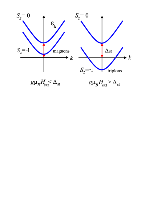
Figure 1: (Color online) Evolution of the magnon states with the increase in the magnetic field. When the bottom of $S_{z}=-1$ band has negative energy, magnons (left panel) become “triplons” (right panel).

Since the triplon BEC occurs in solids, it possesses at least three interesting features resulting from its coupling to the host lattice. First, it is directly influenced by the spin-orbit coupling inherent to the solid where it is located [19]. For atomic BEC the analog of spin-orbit coupling can be produced by special combination of laser fields in some cases [20]. Second, the triplon BEC is coupled to phonons, and, therefore, can provide a test for the effects of decoherence and hysteresis due to the coupling to the lattice [22, 21]. Third, an external pressure applied to the crystal can strongly change the properties of the triplon BEC [23, 24]. In addition, the solid-state background for the triplon BEC makes it accessible by a variety of experimental techniques, not applicable for the atomic condensates.

Theoretical description of triplon BEC in relatively weak fields, where the Zeeman splitting is much less than the width of the triplon band in the Brillouin zone, and, correspondingly, concentration of triplons is small, can be done in terms of weakly interacting Bose gas theory. The observation of the sound-like Bogoliubov spin-flip mode, the fingerprint of the BEC in an interacting Bose gas, in the neutron scattering experiment [25] provided the strong support of this approach to the BEC of triplons.

Main tools for these studies are based on the approach usually referred to as the Hartree-Fock-Popov (HFP) approximation, neglecting the anomalous density terms. The drawback of this approximation is the prediction of a jump in the triplon density, and, in turn, in the sample magnetization across the transition temperature. Although this approach provides a good quantitative description of the specific heat $C_{v}$, it is unclear whether it captures qualitatively all relevant physics of the condensate. For this reason it will be interesting to study the behavior of the triplon BEC using a more accurate approach in order to see whether the analysis beyond the HFP approximation reveals new qualitative features.

In our previous work [26] we have shown that an extended version of the mean field approach (MFA) taking into account anomalous density terms in the condensate, improves the situation considerably [27]. The key part of this approach concentrates on finding the speed of sound-like Bogoliubov excitations in the BEC of interacting particles. This Hartree-Fock-Bogoliubov (HFB) approximation [28] leads to a continuous magnetization across the transition, in agreement with the experiment. By applying this approximation to the BEC of triplons we have shown that when the external magnetic field $H_{\rm ext}$ exceeds a critical value, $H^{\rm cr}_{\rm ext}$, the speed of sound becomes complex and the BEC state undergoes an instability.

Another general feature clearly seen in the triplon BEC is the dependence of its physics on the bare magnon dispersion $\varepsilon_{\mathbf{k}}$. The non-parabolic bare dispersion of magnons [22, 29, 30, 31] leads to a non-trivial dependence of the transition temperature $T_{\rm c}$ on the concentration $\rho\sim M(T,H_{\rm ext})$ and, hence, on $H_{\rm ext}$. The bare dispersion, being itself $H_{\rm ext}$-independent, determines the interplay of kinetic and potential energy of a macroscopic system, and, therefore, plays a crucial role in the BEC properties. The effects of the bare dispersion are clearly seen experimentally in TlCuCl₃ as the $\rho$-dependence $T_{\rm c}\sim\rho^{\phi(\rho)}$. The exponent ${\phi(\rho)}$ approaches $2/3$ at low concentrations (low $T_{c}$),[32] as expected for the parabolic $\varepsilon_{k}\sim k^{2}$, while at $T>2.5$ K, $\phi(\rho)$ is close to 0.5. We will address the role of the dispersion below in the paper and present simplified for the parabolic dispersion calculations.

In this paper we address the macroscopic properties of the BEC in terms of the speed of sound, specific heat, and magnetic susceptibility, in the HFB approximation and show both the quantitative and qualitative importance of the anomalous averages. This paper is organized in the following way. In Section II we outline main features of the HFB approximation. In Section III we discuss the specific heat and magnetic susceptibility in this approximation and show the importance of the anomalous averages. In Section IV we provide a detailed analysis of the instability caused by external magnetic field in terms of the speed of sound and magnetization. This instability is the qualitative effect, not expected if the anomalous averages are not taken into account. The Conclusions summarize our results.

2 The Hartree-Fock-Bogoliubov approximation.

We begin with the Hamiltonian of triplons as a nonideal Bose gas with contact repulsive interaction:

$$\small H=\int d^{3}r\left[\psi^{\dagger}(\mathbf{r})\left(\hat{K}-\mu\right)\psi(\mathbf{r})+\frac{U}{2}\left(\psi^{\dagger}(\mathbf{r})\psi(\mathbf{r})\right)^{2}\right],$$ (1)

where $\psi(\mathbf{r})$ is the bosonic field operator, $U$ is the interaction strength, and $\hat{K}$ is the kinetic energy operator which defines the bare triplon dispersion $\varepsilon_{\mathbf{k}}$ in momentum space. Since the triplon BEC occurs in solids, we perform integration over the unit cell of the crystal with the corresponding momenta defined in the first Brillouin zone. Below the spectrum will be assumed isotropic: $\varepsilon_{\mathbf{k}}=\varepsilon(k)$. The parameter $\mu$ characterizes an additional direct contribution to the triplon energy due to the external field and being rewritten as

$$\small\mu=g\mu_{B}H_{\rm ext}-\Delta_{\rm st}$$ (2)

can be interpreted as a chemical potential of the $S_{z}=-1$ triplons [9]. In Eq. (2) $g$ is the electron Landé factor, $\mu_{B}$ is the Bohr magneton and $\Delta_{\rm st}$ is the spin gap separating the singlet ground state from the lowest-energy triplet excitation (Fig.1).

In general the Hamiltonian in (1) is invariant under global $U(1)$ gauge transformation

$$\small\psi({\mathbf{r}})\rightarrow e^{i\alpha}\psi({\mathbf{r}})$$ (3)

with $\alpha$ being a real number. However, this symmetry is broken in the condensed phase, where $T\leq T_{c}$, and restored for the normal phase, $T>T_{c}$. Note that in the experimental studies of BEC of atomic gases the density $\rho$ (or equivalently, the total number of atoms) is fixed initially and the chemical potential $\mu$ should be calculated self-consistently, while in the case of triplon BEC the chemical potential is fixed by the magnetic field and the density should be determined within an appropriate approximation.

Here and below we adopt the units $k_{B}\equiv 1$ for the Boltzmann constant, $\hbar\equiv 1$ for the Planck constant, and $V\equiv 1$ for the unit cell volume. In these units the energies are measured in Kelvin, the mass $m$ is expressed in K^-1, the magnetic susceptibility $\chi$ for the magnetic fields measured in Tesla has the units of K/T², while the momentum and specific heat $C_{v}$ are dimensionless. Particularly, the Bohr magneton is $\mu_{B}={\hbar e}/{2m_{0}c}=0.671668$ K/T, where $m_{0}$ is the free electron mass, and $e$ is the fundamental charge.

2.1 Condensate phase $T\leq T_{c}$

As it has been shown by Yukalov [28] the spontaneous gauge symmetry breaking is the necessary and sufficient condition for Bose-Einstein condensation and can be realized by the Bogoliubov shift in the field operator as

$$\small\psi({\mathbf{r}})=v({\mathbf{r}})+\widetilde{\psi}({\mathbf{r}}),$$ (4)

where for the uniform case the function $v({\mathbf{r}})$ is a constant defining the density of condensed particles as

$$\small\rho_{0}=v^{2}$$ (5)

Since by the definition of the average of $\psi^{\dagger}({\mathbf{r}})\psi({\mathbf{r}})$ is the total number of particles:

$$\small N=\int_{V}d^{3}r\langle\psi^{\dagger}(\mathbf{r})\psi(\mathbf{r})\rangle.$$ (6)

with the density of triplons per unit cell $\rho=N/V$, from normalization condition

$$\small\rho=\rho_{0}+\rho_{1}$$ (7)

one immediately obtains

$$\small\rho_{1}=\displaystyle\frac{1}{V}\int_{V}d^{3}r\langle\widetilde{\psi}^{\dagger}(\mathbf{r})\widetilde{\psi}(\mathbf{r})\rangle.$$ (8)

Therefore the field operator $\widetilde{\psi}(\mathbf{r})$ determines the density of uncondensed particles. Note that $\widetilde{\psi}(\mathbf{r})$ and the condensate function should be considered as independent variables being orthogonal to each other in terms of the expectation values:

$$\small\int d^{3}r\widetilde{\psi}({\mathbf{r}})v({\mathbf{r}})=0.$$ (9)

Consequently, passing to the momentum space

$$\small\displaystyle\widetilde{\psi}(\mathbf{r})=\sum_{\mathbf{k}}a_{\mathbf{k}}e^{i\mathbf{k}\mathbf{r}}\equiv\int\frac{d^{3}{k}}{(2\pi)^{3}}a_{\mathbf{k}}e^{i\mathbf{k}\mathbf{r}}$$ (10)

and inserting (10) into (8) one can easily see that in (10) the summation by momentum in the finite volume should not include $\mathbf{k=0}$ states. Below we indicate this rule by introducing prime sign in the momentum summation.

Now using (4) and (10) in (1) we present the Hamiltonian as the sum of five terms

$$\displaystyle H=\sum_{n=0}^{4}H_{n},$$ (11)

labeled according to their order with respect to $a_{\mathbf{k}}$ and $a^{\dagger}_{\mathbf{k}}$. The zero-order term does not contain the field operators of uncondensed triplons

$$\displaystyle H_{0}=\frac{U}{2}\rho_{0}^{2}-\mu\rho_{0}.$$ (12)

The first order term is identically zero

$$\small H_{1}=0,$$ (13)

due to the orthogonality condition (8). The second-order term is

$$\displaystyle H_{2}=\sum_{\mathbf{k}}^{\prime}\left[\left(\varepsilon_{k}-\mu+2U\rho_{0}\right)a_{\mathbf{k}}^{\dagger}a_{\mathbf{k}}+\frac{U\rho_{0}}{2}\left(a_{\mathbf{k}}a_{-{\mathbf{k}}}+a_{\mathbf{k}}^{\dagger}a_{-{\mathbf{k}}}^{\dagger}\right)\right].$$ (14)

The third-order

$$\displaystyle H_{3}=U\sqrt{\rho_{0}}\sum_{\mathbf{k,p}}\left(a_{\mathbf{p}}^{\dagger}a_{\mathbf{p-k}}a_{\mathbf{k}}+a_{\mathbf{k}}^{\dagger}a_{\mathbf{p-k}}^{\dagger}a_{\mathbf{p}}\right)$$ (15)

as well as fourth-order

$$\displaystyle H_{4}=\frac{U}{2}\sum_{\mathbf{k,p,q}}^{\prime}a_{\mathbf{k}}^{\dagger}a_{\mathbf{p}}^{\dagger}a_{\mathbf{q}}a_{\mathbf{k+p-q}}$$ (16)

terms are rather complicated and a diagonalization procedure is needed. For this purpose in HFB approximation the following procedure is usually implemented [33]:

$$a_{\mathbf{k}}^{\dagger}a_{\mathbf{p}}a_{\mathbf{q}}\rightarrow 2\langle a_{\mathbf{k}}^{\dagger}a_{\mathbf{p}}\rangle a_{\mathbf{q}}+a_{\mathbf{k}}^{\dagger}\langle a_{\mathbf{p}}a_{\mathbf{p}}\rangle,$$ (17)

$$a_{\mathbf{k}}^{\dagger}a_{\mathbf{p}}^{\dagger}a_{\mathbf{q}}a_{\mathbf{m}}\rightarrow 4a_{\mathbf{k}}^{\dagger}a_{\mathbf{m}}\langle a_{\mathbf{p}}^{\dagger}a_{\mathbf{q}}\rangle+a_{\mathbf{q}}a_{\mathbf{m}}\langle a_{\mathbf{k}}^{\dagger}a_{\mathbf{p}}^{\dagger}\rangle+a_{\mathbf{k}}^{\dagger}a_{\mathbf{p}}^{\dagger}\langle a_{\mathbf{q}}a_{\mathbf{m}}\rangle-2\rho_{1}^{2}-\sigma^{2},$$ (18)

where $\langle a_{\mathbf{k}}^{\dagger}a_{\mathbf{p}}\rangle=\delta_{\mathbf{k},\mathbf{p}}n_{\mathbf{k}},\quad\langle a_{\mathbf{k}}a_{\mathbf{p}}\rangle=\delta_{\mathbf{k},-\mathbf{p}}\sigma_{\mathbf{k}}$ with $n_{\mathbf{k}}$ and $\sigma_{\mathbf{k}}$ being related to the normal ($\rho_{1}$) and anomalous ($\sigma$) densities as

$$\displaystyle\rho_{1}=\sum_{\mathbf{k}}n_{\mathbf{k}},\qquad\displaystyle\sigma=\sum_{\mathbf{k}}\sigma_{\mathbf{k}}.$$ (19)

Here we underline that the main difference between the HFP and HFB approximations concerns the anomalous density: neglecting $\sigma$ as well as $\langle a_{\mathbf{k}}a_{\mathbf{p}}\rangle$ in (14), (17), and (18) one arrives at the HFP approximation, which can also be obtained in variational perturbation theory [34]. However, the normal, $\rho_{1}$, and anomalous averages, $\sigma$, are equally important and neither of them can be neglected without making the theory not self-consistent [35, 36, 37]. Altough $\rho_{1}$ and $\sigma$ are functions of temperature and external magnetic field, we omit explicit dependences in the formulas when it does not cause a confusion.

Taking into account that $E_{3}=\langle H_{3}\rangle=0$, the expectation value of the energy can be evaluated as $E(T\leq T_{c})=E_{0}+E_{2}$, where

$$\small E_{0}=\displaystyle\frac{U\rho_{0}^{2}}{2}-\mu\rho_{0}-\displaystyle\frac{U}{2}(2\rho_{1}^{2}+\sigma^{2}),$$ (20)

and $E_{2}=\langle\widetilde{H}_{2}\rangle$, with $\widetilde{H}_{2}$ being quadratic in $a_{\mathbf{k}},a_{\mathbf{k}}^{\dagger}$:

$$\displaystyle\widetilde{H}_{2}=\sum_{\mathbf{k}}\left[\omega_{k}a_{\mathbf{k}}^{\dagger}a_{\mathbf{k}}+\frac{\Delta}{2}\left(a_{\mathbf{k}}a_{-{\mathbf{k}}}+a_{\mathbf{k}}^{\dagger}a_{-{\mathbf{k}}}^{\dagger}\right)\right].$$ (21)

In the last equation

$$\omega_{k}=\varepsilon_{k}-\mu_{\rm eff},\quad\mu_{\rm eff}=\mu-2U\rho,$$ (22)

$$\Delta=U(\rho_{0}+\sigma).$$ (23)

The next step, in both approximations, is the Bogoliubov transformation

$$a_{\mathbf{k}}=u_{\mathbf{k}}b_{\mathbf{k}}+v_{\mathbf{k}}b_{-{\mathbf{k}}}^{\dagger},\quad a_{\mathbf{k}}^{\dagger}=u_{\mathbf{k}}b_{\mathbf{k}}^{\dagger}+v_{\mathbf{k}}b_{-{\mathbf{k}}}$$ (24)

to diagonalize $\widetilde{H}_{2}$. The operators $b_{\mathbf{k}}$ and $b_{\mathbf{k}}^{\dagger}$ can be interpreted as annihilation and creation operators of phonons with following properties:

$$[b_{\mathbf{k}},b_{\mathbf{p}}^{\dagger}]=\delta_{\mathbf{k},\mathbf{p}},\quad\langle b_{\mathbf{k}}^{\dagger}b_{-{\mathbf{k}}}^{\dagger}\rangle=\langle b_{\mathbf{k}}b_{-\mathbf{k}}\rangle=0,$$ (25)

$$\langle b_{\mathbf{k}}^{\dagger}b_{\mathbf{k}}\rangle=f_{B}(E_{k})=\displaystyle\frac{1}{e^{\beta E_{k}}-1},$$ (26)

where $\beta\equiv 1/T$. To determine the phonon dispersion $E_{k}$ we insert (24) into (21) and require that the coefficient of the term $b_{\mathbf{k}}b_{-\mathbf{k}}+b_{-\mathbf{k}}^{\dagger}b_{\mathbf{k}}^{\dagger}$ vanishes, i.e:

$$\omega_{k}u_{\mathbf{k}}v_{\mathbf{k}}+\frac{\Delta}{2}\left(u^{2}_{\mathbf{k}}+v_{\mathbf{k}}^{2}\right)=0.$$ (27)

Now using the condition $u_{\mathbf{k}}^{2}-v_{\mathbf{k}}^{2}=1$ and presenting $u_{\mathbf{k}},v_{\mathbf{k}}$ as

$$u_{\mathbf{k}}^{2}=\frac{\omega_{k}+E_{k}}{2E_{k}},\quad\quad v_{\mathbf{k}}^{2}=\frac{\omega_{k}-E_{k}}{2E_{k}}$$ (28)

yields

$$\sqrt{\omega_{k}^{2}-E_{k}^{2}}=-\Delta$$ (29)

that is

$$E_{k}=\sqrt{(\omega_{k}+\Delta)(\omega_{k}-\Delta)}$$ (30)

where $\omega_{k}$ and $\Delta$ are given in Eqs. (22) and (23).

Further requirement for $E_{k}$ follows from the Hugenholtz-Pines theorem [38]: at small momentum $k$ the spectrum should be gapless, and, therefore, the phonon dispersion is linear: $E_{k}\sim ck+O(k^{2})$, where $c$ can be considered as the sound speed. This linearity can be achieved by setting

$$\small\omega_{k}-\Delta=\varepsilon_{k},$$ (31)

which together with Eq.(23) yields

$$\small\mu_{\rm eff}=\mu-2U\rho=-\Delta.$$ (32)

With this choice one obtains

$$\small E_{k}=\sqrt{\varepsilon_{k}}\sqrt{\varepsilon_{k}+2\Delta},$$ (33)

with the sound speed

$$\small c=\sqrt{\frac{\Delta}{m}},$$ (34)

i.e. $\Delta=mc^{2}$. Here $m$ has the meaning of the triplon effective mass, characterizing the dispersion in the limit of small momenta $\varepsilon_{k}\approx k^{2}/2m$.

2.2 Condensed fraction and the condensate energy.

Having fixed $u_{\mathbf{k}}$ and $v_{\mathbf{k}}$ one can find normal and anomalous densities as well as the energy by using equations (19)-(28). For example, inserting (24) into (19) results in

$$\displaystyle\sigma=\sum_{\mathbf{k}}\langle a_{\mathbf{k}}a_{-{\mathbf{k}}}\rangle=\sum_{\mathbf{k}}u_{\mathbf{k}}v_{\mathbf{k}}(1+2f_{B}(E_{k}))=-\Delta\sum_{\mathbf{k}}\displaystyle\frac{W_{k}}{E_{k}},$$ (35)

where we used the relation $u_{\mathbf{k}}v_{\mathbf{k}}=-{\Delta}/{2E_{k}}$ and introduced notation $W_{k}={1}/{2}+f_{B}(E_{k})$. Similarly one obtains:

$$\displaystyle\rho_{1}=\sum_{\mathbf{k}}\langle a_{\mathbf{k}}^{\dagger}a_{\mathbf{k}}\rangle=\sum_{\mathbf{k}}\left(\displaystyle\frac{W_{k}\omega_{k}}{E_{k}}-\displaystyle\frac{1}{2}\right),$$ (36)

$$E_{2}=\langle\widetilde{H}_{2}\rangle=\sum_{\mathbf{k}}E_{k}f_{B}(E_{k})+\displaystyle\frac{1}{2}\sum_{\mathbf{k}}(E_{k}-\omega_{k}),$$ (37)

with  $\omega_{k}=\varepsilon_{k}+\Delta$.

When the bare dispersion $\varepsilon_{k}$ is isotropic, the momentum summation can be done with:

$$\small\sum_{\mathbf{k}}f\left({k}^{2}\right)=\displaystyle\frac{4\pi}{\left(2\pi\right)^{3}}\int_{0}^{\infty}f\left({k}^{2}\right)k^{2}dk.$$ (38)

As a result, at $T=0$ the quantities in Eqs.(35)-(37) can be represented as:

$$\rho_{1}(0)=\displaystyle\frac{1}{2}\sum_{\mathbf{k}}\left(\displaystyle\frac{\varepsilon_{k}+\Delta}{E_{{k}}}-1\right)=\displaystyle\frac{1}{4\pi^{2}}\int_{0}^{\infty}{k^{2}dk}\left(\displaystyle\frac{\varepsilon_{k}+\Delta}{E_{{k}}}-1\right)$$ (39)

$$\sigma(0)=-\displaystyle\frac{\Delta}{4\pi^{2}}\int_{0}^{\infty}\displaystyle\frac{k^{2}dk}{E_{k}}$$ (40)

$$E_{2}(0)=\displaystyle\frac{1}{4\pi^{2}}\left(\int_{0}^{\infty}E_{{k}}k^{2}dk-\int_{0}^{\infty}\left(\varepsilon_{{k}}+\Delta\right)k^{2}dk\right),$$ (41)

The divergences in these integrals can be regularized by introducing a cutting parameter $\Lambda$ ($\Lambda\rightarrow\infty$ at the end of the calculations) or equivalently by using the dimensional regularization scheme. Now, assuming for the moment that, for $T=0$ case $\varepsilon_{k}={k}^{2}/{2m}$ and using dimensional regularization one obtains:

$$\rho_{1}(0) = \displaystyle\frac{(\Delta m)^{3/2}}{3\pi^{2}},$$ (42)

$$\sigma(0) = 3\rho_{1}(0),$$ (43)

$$E_{2}(0) = \displaystyle\frac{8(\Delta m)^{5/2}}{15m\pi^{2}}.$$ (44)

Summarizing this subsection we rewrite the above formulas as:

$$\rho_{1} = \displaystyle\frac{(\Delta m)^{3/2}}{3\pi^{2}}+\displaystyle\int\displaystyle\frac{d^{3}{k}}{\left(2\pi\right)^{3}}f_{B}(E_{{k}})\displaystyle\frac{\varepsilon_{k}+\Delta}{E_{k}},$$ (45)

$$\sigma = \displaystyle\frac{(\Delta m)^{3/2}}{\pi^{2}}-\Delta\displaystyle\int\displaystyle\frac{d^{3}{k}}{\left(2\pi\right)^{3}}f_{B}(E_{{k}})\displaystyle\frac{1}{E_{{k}}},$$ (46)

$$E = \displaystyle\frac{8(\Delta m)^{5/2}}{15m\pi^{2}}+\displaystyle\frac{U\rho_{0}^{2}}{2}-\mu\rho_{0}-\displaystyle\frac{U}{2}\left(2\rho_{1}^{2}+\sigma^{2}\right)+\displaystyle\int\displaystyle\frac{d^{3}{k}}{\left(2\pi\right)^{3}}E_{{k}}f_{B}\left(E_{{k}}\right),$$ (47)

where Bose distribution of phonons $f_{B}\left(E_{{k}}\right)$ is defined in Eq.(26).

To perform the MFA calculations one starts by solving Eqs. (23) and (32) with $\rho_{1}$ and $\sigma$ given by Eqs. (45) and (46). As outlined above, in contrast to the BEC of atomic gases, in the triplon problem the chemical potential $\mu$ is the input parameter, whereas the densities are the output ones. Bearing this in mind, we rewrite the main Eqs. (23) and (32) as

$$\Delta = \mu+2U\left(\sigma-\rho_{1}\right),$$ (48)

$$\rho_{0} = {\Delta}/{U}-\sigma.$$ (49)

The system of coupled equations, (45), (46) and (48), (49) has to be solved for given  $T$ and $\mu$ to evaluate the triplon density

$$\small\rho(T\leq T_{c})=\rho_{0}+\rho_{1}=\displaystyle\frac{\Delta+\mu}{2U},$$ (50)

which is proportional to the measured sample magnetization density $M$. Note that by formally setting in all above formulas $\sigma\equiv 0$, one arrives at the HFP approximation and particularly

$$\Delta=\mu-2U\rho_{1},\qquad\rho_{0}={\Delta}/{U}.$$ (51)

2.3 The critical temperature and triplon density

Before discussing the normal $T>T_{c}$ phase we evaluate the temperature of BEC transition. It is well-known that in the MFA the system of interacting Bose condensate particles at $T\rightarrow T_{c}$ behaves like an ideal gas. In fact, assuming $\rho_{0}(T\rightarrow T_{c})=0$, $\rho_{1}(T\rightarrow T_{c})=\rho_{c}$, $\sigma(T\rightarrow T_{c})=0$, $\Delta(T\rightarrow T_{c})=0$, and $E_{k}=\varepsilon_{k}$ one concludes from Eqs.(45),(48) that

$$\small\rho_{c}=\displaystyle\int\displaystyle\frac{d^{3}{k}}{(2\pi)^{3}}\displaystyle\frac{1}{\exp(\beta_{c}\varepsilon_{k})-1}=\displaystyle\frac{\mu}{2U}.$$ (52)

With given $\mu=\mu_{B}gH_{\rm ext}-\Delta_{\rm st}$ and coupling constant $U$, the critical temperature $T_{c}\equiv 1/\beta_{c}$ can be found as a solution of Eq. (52). Note that for the parabolic dispersion $\varepsilon_{k}=k^{2}/{2m}$, the integral (52) can be evaluated analytically giving following well known relation [42]:

$$\small T_{c}^{\rm[par]}=\displaystyle\frac{2\pi}{m}\;\left(\displaystyle\frac{\mu}{2\zeta(3/2)U}\right)^{2/3},$$ (53)

where $\zeta(x)$ is the Riemann function.

As it has been underlined in Introduction, the bare dispersion of magnons, $\varepsilon_{k}$, plays the crucial role in determining $T_{c}$. Figure 2 presents the transition temperature as a function of magnetic field $H_{\rm ext}$ and corresponding triplon density $\rho$, that is the sample magnetization, for parabolic $\varepsilon_{k}={k}^{2}/{2m}$ and ”relativistic”

$$\small\varepsilon_{k}=\sqrt{\Delta_{\rm st}^{2}+J^{2}k^{2}/4}-\Delta_{\rm st}$$ (54)

bare dispersion, typical for a system with a gapped spectrum [24, 43]. Here the effective exchange parameter $J=2\sqrt{\Delta_{\rm st}/m}$ is chosen to match the parabolic and the relativistic $\varepsilon_{k}$ at small $k$. The dashed line obtained directly from Eq.(53) displays $T_{c}\sim\rho^{2/3}$ behavior. The solid one is a result of numerical solution of Eq.(52) with the dispersion in Eq.(54) and shows a crossover from $T_{c}\sim\rho^{2/3}$ at lower to $T_{c}\sim\rho^{0.5}$ at higher temperatures in agreement with the experimental data. The decrease in $\Delta_{\rm st}$ enhances the role of relativistic features in the spectrum and leads to a faster deviation from the $T_{c}\sim\rho^{2/3}$ behavior, as can be seen in Fig.2. Here and below we mainly use the set of input parameters as $m=0.0204$ K^-1, $\Delta_{\rm st}=7.1$ K, $U=313$ K, and $g=2.06$ [32] valid for the weakly anisotropic quantum antiferromagnet TlCuCl₃.

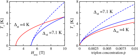
Figure 2: (Color online) The critical temperature of BEC of triplons $T_{c}$ as a function of external field (left panel) and corresponding triplon density $\rho=\mu/2U$ (right panel) for two values of the singlet-triplet gap. To understand the role of the gap in the magnon spectrum, we present the results for $\Delta_{\rm st}=4$ K, with the reduced exchange parameter yielding the same effective mass as for $\Delta_{\rm st}=7.1$ K. The gap values are marked near the lines. The solid and dashed lines are for the relativistic and parabolic dispersions for $\Delta_{\rm st}=7.1$ K, respectively.

In the normal phase the symmetry in Eq.(3) is not broken and the Bogoliubov shift is not needed either. Here the anomalous density vanishes, $\sigma(T>T_{c})=0$, and hence, both approximations, HFB and HFP coincide. As a result we obtain for the triplon density

$$\small\begin{array}[]{l}\rho(T>T_{c})=\displaystyle\int\displaystyle\frac{d^{3}{k}}{\left(2\pi\right)^{3}}\displaystyle\frac{1}{\exp\left(\beta\omega_{k}\right)-1}\\ \end{array}$$ (55)

with $\omega_{k}=\varepsilon_{k}-\mu+2U\rho\equiv\varepsilon_{k}-\mu_{\rm eff}$. Similarly, by setting $\Delta=\rho_{0}=\sigma=0,\ \rho_{1}=\rho,\ E_{{k}}=\omega_{{k}}$ in Eq.(47) one obtains following equation for the energy per unit cell

$$\small E(T>T_{c})=-U\rho^{2}+\displaystyle\int\displaystyle\frac{d^{3}{k}}{\left(2\pi\right)^{3}}\frac{\omega_{k}}{\exp\left(\beta\omega_{k}\right)-1}.$$ (56)

The density of triplons as a function of temperature, evaluated in the HFP and HFB approximations is presented in Fig.3. It is seen that the former leads to a discontinuity in the magnetization near the critical temperature, while the latter gives a continuous behavior in accordance with the experimental data [32, 44]. However, in the condensate phase, the triplon density is higher in the HFB than in the HFP approximation. Therefore, the validity of the description of the BEC in the HFP approximation can be checked in the magnetization measurement experiments.

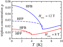
Figure 3: (Color online). Comparison of the HFB (solid lines) and the HFP (dashed lines) results for the triplon density. The HFB approach shows a continuous behavior, which fully agrees with the experimental data [32, 44] while the HFP approach leads to the discontinuity. The corresponding magnetic fields $H_{\rm ext}$ are marked near the plots.

3 Macroscopic properties: specific heat and magnetic susceptibility

3.1 General expressions with nonzero anomalous averages

Triplon contribution to the constant volume specific heat $C_{v}$, can be calculated by differentiation of the energy with respect to the temperature at given chemical potential, that is at given external field [45, 46]:

$$\small C_{v}(H_{\rm ext},T)=\displaystyle\frac{\partial E}{\partial T},$$ (57)

where the energies for condensate and normal states are given by Eqs. (47) and (56), respectively.

Before discussing the magnetic susceptibility, we note that the macroscopic properties of the systems are related to their response to external fields. An example is given by the isothermal compressibility

$$\small\kappa_{T}=-\displaystyle\frac{1}{V}{\left(\displaystyle\frac{\partial V}{\partial P}\right)}_{T}=\displaystyle\frac{1}{\rho}{\left(\displaystyle\frac{\partial\rho}{\partial P}\right)}_{T}.$$ (58)

If $\kappa_{T}\rightarrow\infty$ the system becomes unstable [46, 47] since an infinitesimal fluctuation of pressure $P$ will lead to its collapse or explosion. As to the triplons their density is proportional to the magnetization $M$, while the $H_{\rm ext}$ simulates the pressure, and hence the relevant parameter, which determines the stability of the system with respect to the magnetic field, is the susceptibility

$$\small\chi(H_{\rm ext},T)=\left(\displaystyle\frac{\partial M}{\partial H_{\rm ext}}\right)_{T}.$$ (59)

The susceptibility can be calculated with the triplon density as:

$$\small\chi(H_{\rm ext},T)=(g\mu_{B})^{2}\displaystyle\frac{\partial\rho}{\partial\mu}.$$ (60)

We will omit $H_{\rm ext}$ from the arguments of $\chi(H_{\rm ext},T)$ and $C_{v}(H_{\rm ext},T)$ below.

We begin with the normal phase, where $\rho_{0}=\sigma=\Delta=0$. The derivative of the density with respect to the temperature can be evaluated here with Eq.(LABEL:2.50) as

$$\small\frac{\partial\rho}{\partial T}=\displaystyle\frac{\beta S_{1}}{2S_{2}-1}.$$ (61)

Calculating the derivative of Eq.(56) with respect to $T$ one obtains:

$$\small C_{v}(T>T_{c})=-S_{3}+2US_{1}\frac{\partial\rho}{\partial T}.$$ (62)

Here we introduced dimensionless quantities

$$\small S_{1}=\sum_{\mathbf{k}}\omega_{k}f_{B}^{\prime}\left(\omega_{k}\right),\quad S_{2}=U\sum_{\mathbf{k}}f_{B}^{\prime}\left(\omega_{k}\right),\quad S_{3}=\beta\sum_{\mathbf{k}}\omega_{k}^{2}f_{B}^{\prime}\left(\omega_{k}\right),$$ (63)

and used the relation ${\partial f_{B}(\omega)}/{\partial T}=-\beta\omega f_{B}^{\prime}(\omega)$, where $f_{B}^{\prime}\left(\omega\right)={\partial f_{B}(\omega)}/{\partial\omega}=-\beta\exp({\beta\omega})f_{B}^{2}\left(\omega\right)$ and $\omega_{k}$ is given in Eq.(22).

Similarly, taking the derivative of the self-consistency Eq.(LABEL:2.50), which we present here in the form:

$$\rho(\mu)=\sum_{\mathbf{k}}\displaystyle\frac{1}{\exp\left[\beta\left(\varepsilon_{k}-\mu+2U\rho(\mu)\right)\right]-1}$$ (64)

with respect to $\mu$ and solving the equation for $\partial\rho/\partial\mu$ one finds $\partial\rho/\partial\mu=S_{2}/U(2S_{2}-1)$. As a result, we obtain with Eq.(60) the normal phase susceptibility:

$$\chi(T>T_{c})=\frac{\left(g\mu_{B}\right)^{2}}{U}\displaystyle\frac{S_{2}}{2S_{2}-1}.$$ (65)

Now we proceed with the condensate phase, where the dependence of $\Delta$ and the corresponding normal and anomalous densities on temperature and magnetic field should be taken into account.

Here $C_{v}(T)$ is obtained by taking the derivative of $E\left(T<T_{c}\right)$ given by Eq. (47). The latter can be rewritten as:

$$E\left(T<T_{c}\right)={E}_{2}-\displaystyle\frac{\mu^{2}}{2U}+U\left(\rho_{1}^{2}-2\rho_{1}\sigma\right),$$ (66)

where we used the relation $\rho_{0}=\mu/U-2\rho_{1}+\sigma$ and present ${E}_{2}$ defined in Eq.(37) as:

$${E}_{2}=\displaystyle\frac{8m^{3/2}\Delta^{5/2}}{15\pi^{2}}+\sum_{\mathbf{k}}E_{k}f_{B}\left(E_{k}\right).$$ (67)

As a result:

$$C_{v}(T\leq T_{c})=\displaystyle\frac{\partial E_{2}}{\partial T}-2U\rho_{1}\displaystyle\frac{\partial\sigma}{\partial T}-2U\left(\rho-\displaystyle\frac{\mu}{U}\right)\displaystyle\frac{\partial\rho_{1}}{\partial T}.\\$$ (68)

We begin with calculation of ${\partial\Delta}/{\partial T}$, which is the key ingredient in the specific heat. It is obtained by differentiating both sides of the main equation (48) with respect to the temperature, and for known ${\partial\Delta}/{\partial T}$ the other two derivatives ${\partial\rho_{1}}/{\partial T}$ and ${\partial\sigma}/{\partial T}$ can be evaluated directly from Eqs.(45), (46). As a result one obtains the derivatives necessary to evaluate the specific heat:

$$\displaystyle\frac{\partial\Delta}{\partial T}=\displaystyle\frac{2U\beta}{1-2U\left(\displaystyle\frac{\sqrt{\Delta}m^{3/2}}{\pi^{2}}-\sum_{\mathbf{k}}{\cal F}\left(E_{k}\right)\right)}\sum_{\mathbf{k}}\left(\varepsilon_{k}+2\Delta\right)f_{B}^{\prime}(E_{k}),$$ (69)

$$\displaystyle\frac{\partial\rho_{1}}{\partial T}=\displaystyle\frac{m\sqrt{\Delta m}}{2\pi^{2}}\frac{\partial\Delta}{\partial T}+\sum_{\mathbf{k}}\left[\displaystyle\frac{\partial\Delta}{\partial T}\left(\displaystyle\frac{\varepsilon_{k}\Delta}{E_{k}^{2}}{\cal F}\left(E_{k}\right)+\displaystyle\frac{\varepsilon_{k}^{2}}{E_{k}^{2}}f_{B}^{\prime}\right)-\beta\left(\varepsilon_{k}+\Delta\right)f_{B}^{\prime}(E_{k})\right],$$ (70)

$$\displaystyle\frac{\partial\sigma}{\partial T}=\displaystyle\frac{3m\sqrt{\Delta m}}{2\pi^{2}}\frac{\partial\Delta}{\partial T}-\sum_{\mathbf{k}}\left[\frac{\partial\Delta}{\partial T}\left(\displaystyle\frac{\varepsilon_{k}\Delta}{E_{k}^{2}}{\cal F}\left(E_{k}\right)+\displaystyle\frac{\varepsilon_{k}^{2}}{E_{k}^{3}}f_{B}(E_{k})\right)-\beta\Delta f_{B}^{\prime}(E_{k})\right],$$ (71)

where we introduced notation for the frequently used expression:

$${\cal F}\left(E_{k}\right)\equiv\displaystyle\frac{f_{B}(E_{k})}{E_{k}}+f_{B}^{\prime}(E_{k}).$$ (72)

The expression for

$$\frac{\partial E_{2}}{\partial T}=\displaystyle\frac{4\left(\Delta m\right)^{3/2}}{3\pi^{2}}\displaystyle\frac{\partial\Delta}{\partial T}+\sum_{\mathbf{k}}\left(\frac{\partial\Delta}{\partial T}\varepsilon_{k}{\cal F}\left(E_{k}\right)-\beta E_{k}^{2}f_{B}^{\prime}(E_{k})\right)$$ (73)

completes the set of derivatives necessary for evaluation of the specific heat.

The derivative ${\partial\Delta}/{\partial\mu}$ can be found by differentiating both sides of the main equation (48) with respect to $\mu$. As a result,

$$\frac{\partial\Delta}{\partial\mu}=\displaystyle\frac{1}{1-2U\left(\displaystyle\frac{\sqrt{\Delta}m^{3/2}}{\pi^{2}}-\sum_{\mathbf{k}}{\cal F}\left(E_{k}\right)\right)}.$$ (74)

As to ${\partial\rho}/{\partial\mu}$, needed for evaluation of the magnetic susceptibility in Eq.(60), it is obtained by differentiating the equation $\rho=\left(\Delta+\mu\right)/2U,$ with respect to $\mu$. This yields

$$\small\chi(T\leq T_{c})=\displaystyle\frac{\left(g\mu_{B}\right)^{2}}{2U}\left(\displaystyle\frac{\partial\Delta}{\partial\mu}+1\right).$$ (75)

Below we apply these equations to the cusps in the specific heat and susceptibility and to the qualitative effects such as the instability in strong magnetic fields. We will show that at a given temperature, there exists a critical field $H^{\rm cr}_{\rm ext}(T)$, such that when $H_{\rm ext}$ approaches $\geq H^{\rm cr}_{\rm ext}(T)$, the magnetic susceptibility, $\chi(H_{\rm ext},T)$ diverges.

3.2 Cusp in the specific heat and magnetic susceptibility near $T_{c}$

The cusp in the specific heat defined as

$$\Delta C_{v}=\lim_{T\rightarrow T_{c}-0}C_{v}(T)-\lim_{T\rightarrow T_{c}+0}C_{v}(T)$$ (76)

is an interesting quantity in the theory of phase transitions. In accordance with the Ehrenfest classification, a phase transition with the discontinuity in $C_{v}$ near the transition point, is the second order one. Particularly, it is well-known that [45, 46] for the ideal gas $\Delta C_{v}$ near the transition into BEC is zero i.e. the specific heat is continuous. We shall illustrate this fact for completeness. The specific heat per particle of the ideal Bose gas is given by [45, 46]

$$\small\begin{array}[]{l}{C_{v}^{U=0}(T\leq T_{c})}=\displaystyle\frac{15\zeta(5/2)}{4\zeta(3/2)}\left(\displaystyle\frac{T}{T_{c}}\right)^{3/2},\\ \end{array}$$ (77)

$$\small\begin{array}[]{l}{C_{v}^{U=0}(T>T_{c})}=\displaystyle\frac{15g_{5/2}(z)}{4g_{3/2}(z)}-\displaystyle\frac{9g_{3/2}(z)}{4g_{1/2}(z)},\end{array}$$ (78)

where $g_{p}(z)$ is defined as:

$$g_{p}(z)=\displaystyle\frac{1}{\Gamma\left(p\right)}\int_{0}^{\infty}dx\displaystyle\frac{x^{p-1}}{z^{-1}e^{x}-1},$$ (79)

related to the Riemann function as $\zeta(p)=g_{p}(z=1)$. When $T\rightarrow T_{c}+0$, the fugacity $z=\exp({\beta\mu})<1$ tends to unity, i. e. $\displaystyle\lim_{T\rightarrow T_{c}+0}z=1$ and the second term in (78) vanishes, because of the divergence in $g_{1/2}$, i.e. $g_{1/2}(z)\sim(1-z)^{-1/2}$ in this region, while the first term exactly coincides with (LABEL:3.18). As a result,

$$\small\Delta C_{v}^{U=0}=0,$$ (80)

and hence the specific heat of the ideal gas is continuous although being plotted as a function of temperature $C_{v}^{U=0}(T)$ behaves similarly to the $\lambda$ curve.

We proceed with calculation of $\Delta C_{v}$. Bearing in mind that for $T>T_{c}$ HFB and HFP approximations coincide, from (62) we obtain

$$\lim_{T\rightarrow T_{c}+0}C_{v}(T)=-\beta_{c}\sum_{\mathbf{k}}\varepsilon_{k}^{2}f_{B}^{\prime}(\varepsilon_{k}).$$ (81)

For $T<T_{c},$ $C_{v}$ is given by Eqs. (68)-(72). Assuming in the last equations $E_{{k}}=\varepsilon_{k}$ and $\Delta=0,$ one finds

$$\lim_{T\rightarrow T_{c}-0}\frac{\partial\Delta}{\partial T}=\displaystyle\frac{2\beta_{c}U}{1+2U\displaystyle{\sum_{\mathbf{k}}}{\cal F}\left(\varepsilon_{k}\right)}{\sum_{\mathbf{k}}}f_{B}^{\prime}(\varepsilon_{k})\varepsilon_{k},$$ (82)

which is finite. Using (82) in (70)-(72) and setting in (68) $\rho=\mu/2U$, $\rho_{0}=0,\rho_{1}=\rho,\sigma=0$, one obtains for the maximum value of the specific heat $\mbox{max}\{C_{v}^{\rm HFB}(T)\}\equiv\lim_{T\rightarrow T_{c}-0}C_{v}(T)$:

$$\lim_{T\rightarrow T_{c}-0}C_{v}(T)=\sum_{\mathbf{k}}\left(\mu+\varepsilon_{k}\right)\left({\cal F}\left(\varepsilon_{k}\right)\frac{\partial\Delta}{\partial T}-\beta_{c}\varepsilon_{k}f_{B}^{\prime}(\varepsilon_{k})\right).$$ (83)

Subtracting (81) from (83) we finally obtain

$$\Delta C_{v}=\sum_{\mathbf{k}}\left({\cal F}\left(\varepsilon_{k}\right)\left(\mu+\varepsilon_{k}\right)\frac{\partial\Delta}{\partial T}-\mu\beta_{c}\varepsilon_{k}f_{B}^{\prime}(\varepsilon_{k})\right),$$ (84)

where ${\partial\Delta}/{\partial T}$ is given by Eq. (82).

In a quite similar way one can calculate the cusp in the susceptibility:

$$\Delta\chi=\displaystyle\frac{\left({g}\mu_{B}\right)^{2}}{2U}\frac{1}{1+2U\displaystyle{\sum_{\mathbf{k}}}{\cal F}\left(\varepsilon_{k}\right)}.$$ (85)

3.3 Parabolic dispersion, $\varepsilon_{k}={k}^{2}/2m$

For the parabolic dispersion, calculations can be done analytically, as presented below. The specific heat is expressed as:

$$\mbox{max}\{C_{v}(T)\}=-\beta_{c}R_{1}-\mu\beta_{c}R_{2}+\frac{\partial\Delta}{\partial T}\left(R_{2}+\mu R_{3}+R_{5}\right),$$ (86)

$$\lim_{T\rightarrow T_{c}+0}C_{v}(T)=-\beta_{c}R_{1},$$ (87)

$$\Delta C_{v}=\mbox{max}\{C_{v}(T)\}+\beta_{c}R_{1}=\frac{\partial\Delta}{\partial T}\left(R_{2}+\mu R_{3}+R_{5}\right)-\mu\beta_{c}R_{2},$$ (88)

and the cusp in the susceptibility has the form:

$$\Delta\chi=\frac{\left(g\mu_{B}\right)^{2}}{2U}\frac{\partial\Delta}{\partial\mu}.$$ (89)

The derivatives ${\partial\Delta}/{\partial T}$ and ${\partial\Delta}/{\partial\mu}$ can be simplified to:

$$\frac{\partial\Delta}{\partial T} = \displaystyle\frac{2\beta_{c}UR_{2}}{1+2UR_{3}},$$ (90)

$$\frac{\partial\Delta}{\partial\mu} = \displaystyle\frac{1}{1+2UR_{3}}.$$ (91)

In these formulas we used following notations:

$$R_{1} = -\beta_{c}\sum_{\mathbf{k}}f_{B}^{2}(\varepsilon_{k})\varepsilon_{k}^{2}e^{\beta_{c}\varepsilon_{k}}=-\displaystyle\frac{\zeta(5/2)\Gamma\left(7/2\right)}{\sqrt{2}\pi^{2}}T_{c}k_{T}^{3},$$ (92)

$$R_{2} = -\beta_{c}\sum_{\mathbf{k}}f_{B}^{2}(\varepsilon_{k})\varepsilon_{k}e^{\beta_{c}\varepsilon_{k}}=-\displaystyle\frac{\zeta(3/2)\Gamma\left(5/2\right)}{\sqrt{2}\pi^{2}}k_{T}^{3},$$ (93)

$$R_{3} = \sum_{\mathbf{k}}\left(f_{B}^{\prime}(\varepsilon_{k})+f_{B}(\varepsilon_{k})/\varepsilon_{k}\right)=-\displaystyle\frac{0.6471\sqrt{2}}{\pi^{2}}\frac{k_{T}^{3}}{T_{c}},$$ (94)

$$R_{4} = \sum_{\mathbf{k}}f_{B}(\varepsilon_{k})\varepsilon_{k}=\displaystyle\frac{\zeta(5/2)\Gamma\left(5/2\right)}{\sqrt{2}\pi^{2}}T_{c}k_{T}^{3},$$ (95)

$$R_{5} = \sum_{\mathbf{k}}f_{B}(\varepsilon_{k})=\displaystyle\frac{\zeta(3/2)\Gamma\left(3/2\right)}{\sqrt{2}\pi^{2}}k_{T}^{3},$$ (96)

where we introduced $k_{T}\equiv\sqrt{mT_{c}}$ for the characteristic thermal wavevector of triplon at the transition temperature. Taking into account that $R_{5}$ is the triplon concentration, we find that Eq.(96) is equivalent to Eq.(53).

4 High- field instability

It is well-known that [47, 48] the dynamic stability of equilibrium system is determined by its excitation spectrum: When the latter becomes imaginary the time evolution of excitations changes qualitatively. In the condensate state the spectrum is given by $E_{k}=\sqrt{\varepsilon_{k}}\sqrt{\varepsilon_{k}+2\Delta}$ where $\Delta$ is the solution of nonlinear algebraic Eq.(48) which may be rewritten as follows

$$\small\Delta=\mu+\displaystyle\frac{4U(\Delta m)^{3/2}}{3\pi^{2}}-\frac{U}{\pi^{2}}\int_{0}^{\infty}\displaystyle\frac{\varepsilon_{k}+2\Delta}{E_{k}}f_{B}(E_{k})k^{2}dk.$$ (97)

Obviously, for some set of system parameters $U$, $m$ and external fields $H_{\rm ext}$, Eq.(97) may have no real solution and hence the spectrum, as well as the sound speed, become imaginary. For example, in our previous work we have shown that for parameters [32] this may happen, at $H_{\rm ext}^{\rm cr}=12.5$ T at $T=0$ with the increasing in $H_{\rm ext}^{\rm cr}$ with $T$. Below we investigate the magnetic susceptibility near the instability point and show that it goes to infinity, as expected in these cases, providing the direct experimental test for the instability. This effect can be seen from the fact that when $H_{\rm ext}=H_{\rm ext}^{\rm cr}$, i. e. $\mu=\mu_{\rm cr}$ the denominator of Eq. (74) becomes zero, and hence $\partial\Delta/\partial\mu$ diverges. For $\mu>\mu_{\rm cr}$ the main equation (97) has no positive solution and hence the sound speed $c=\sqrt{\Delta}/\sqrt{m}$ becomes complex. Below we illustrate this analytically for $T=0$.

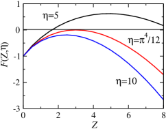
Figure 4: The LHS of Eq. (101) for different values of $\eta$. The real solutions of this equation correspond to the intersection of $F(Z,\eta)$ with the $Z=0$ axis.

For zero temperature the derivative ${\partial\Delta}/{\partial\mu}$ in Eq. (74) is written as

$$\small\frac{\partial\Delta}{\partial\mu}=\displaystyle\frac{1}{1-\displaystyle\frac{2U\sqrt{\Delta}m^{3/2}}{\pi^{2}}},$$ (98)

where $\Delta$ is the solution to the following equation:

$$\small\Delta=\mu+\displaystyle\frac{4U(\Delta m)^{3/2}}{3\pi^{2}}.$$ (99)

Introducing dimensionless variables $\eta=\mu U^{2}m^{3}$ and $Z=\Delta/\mu$ one can rewrite the last two equations as:

$$\frac{\partial\Delta}{\partial\mu}=\displaystyle\frac{1}{1-\displaystyle\frac{2\sqrt{\eta Z}}{\pi^{2}}},$$ (100)

$$F(Z,\eta)\equiv Z-\displaystyle\frac{4Z^{3/2}\sqrt{\eta}}{3\pi^{2}}-1=0,$$ (101)

where $\eta$ is an input parameter. In Fig.4 $F(Z,\eta)$ is plotted as a function of $Z$ for various values of $\eta$. It is seen that for $\eta$ larger than some critical $\eta_{\rm cr}$, the second term in (101) dominates, $F(Z,\eta)$ is always negative, and hence there is no real solutions. If the maximum value of $F(Z,\eta)$, $(\max{F(Z,\eta)})$, for a given $\eta$ is negative the Eq. (101), has no real solution. Otherwise, when $\max(F(Z,\eta)$ is positive, $F(Z,\eta)$ intersects the $Z$-axis and the equation has at least one positive solution. Thus, the boundaries $\eta_{\rm cr}$ and $Z_{\rm cr}$ are defined by the coupled equations:

$$F(Z_{\rm cr},\eta_{\rm cr})=Z_{\rm cr}-\displaystyle\frac{4Z_{\rm cr}^{3/2}\sqrt{\eta_{\rm cr}}}{3\pi^{2}}-1=0,$$ (102)

$$\left.\frac{\partial F}{\partial Z}\right|_{Z=Z_{\rm cr},\eta=\eta_{\rm cr}}=1-\displaystyle\frac{2\sqrt{Z_{\rm cr}\eta_{\rm cr}}}{\pi^{2}}=0,$$ (103)

giving $\eta_{\rm cr}=\pi^{4}/12=8.1174$ and $Z_{\rm cr}=3$. By comparing (103) and (100) one concludes that when $\eta$ approaches $\eta_{\rm cr}$, ${\partial\Delta}/{\partial\mu}$ goes to infinity and so does the magnetic susceptibility given by Eq. (75) i.e. $\chi$ can diverge. When $\eta$ exceeds $\eta_{\rm cr}$, solutions of Eqs. (99), (101) acquire an imaginary part. Bearing in mind that $\eta=\mu m^{3}U^{2}=(\mu_{B}gH_{\rm ext}-\Delta_{\rm st})m^{3}U^{2}$, one concludes that even at $T=0$, if the $H_{\rm ext}$ is strong enough the speed of sound $c=\sqrt{\Delta/m}=\sqrt{\mu Z/m}$ becomes complex and the Bose condensed system of triplons displays dynamical instability. By expanding Eq.(101) in the vicinity of the point $Z=Z_{\rm cr}$,$\eta=\eta_{\rm cr}$, we obtain in this region for the real and imaginary parts of the speed of sound: ${\rm Re}(c)=\sqrt{3\mu_{\rm cr}/m}$ and ${\rm Im}(c)/{\rm Re}(c)=-2\sqrt{\mu-\mu_{\rm cr}}Um^{3/2}/\pi^{2}$, where $\mu_{\rm cr}\equiv\eta_{\rm cr}/(m^{3}U^{2})$.

Similarly it can be shown that for any given $T\leq T_{c}$ there is a maximal value of the external magnetic field $H_{\rm ext}^{\rm cr}$ such that the system posses dynamical instability at this point i.e. $\chi(H_{\rm ext}^{\rm cr},T^{\rm cr})\rightarrow\infty$ and simultaneously the sound speed acquires an imaginary part. This fact is illustrated in Figs.5 and 6. In Fig.5 the susceptibility $\chi(H_{\rm ext},T)$ is plotted as a function of $H_{\rm ext}$. In Fig.6 the solution of the main equation, more precisely, the components of the sound speed $c$ are plotted as a function of $H_{\rm ext}$ for several temperatures. It is clearly seen that for a given temperature the $\chi(H_{\rm ext},T)$ diverges and the sound speed becomes complex at the same $H_{\rm ext}$.

Note that in the HFP approximation Eq.(101) being written as

$$\small F_{\rm HFP}(Z,\eta)=Z+\displaystyle\frac{2Z^{3/2}\sqrt{\eta}}{3\pi^{2}}-1=0$$ (104)

has a positive solution for any positive $\eta$. Thus this approximation precludes the appearance of the instability.

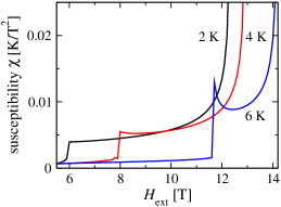
Figure 5: The magnetic susceptibility $\chi(T,H_{\rm ext})$ for the temperatures marked near the plots. When external magnetic field reaches the critical value $H_{\rm ext}^{\rm cr}$ the susceptibility diverges.

The experiment related results from the observed instability are presented in Fig.5 and Fig.6. Figure 5 shows the divergence of the susceptibility. Figure 6 shows how the imaginary part in the velocity appears and the real part of the velocity changes if the field becomes stronger than the threshold value. This is a qualitative effect, which should demonstrate itself in the experiment. Here an important comment on the values of the fields where the singular behavior of $\Delta$ can be observed is in order. A comparison of the calculations presented in Fig.3, experimental results [32, 44], and theory taking into account the exact spectrum of triplons [29], shows that our model spectrum leads to an overestimate of the tiplon concentration by about a factor of 1.5. Therefore, it underestimates the threshold field, leading to the result that fields of the order of 20 T will be necessary [49] to put the condensate in the unstable part of the phase diagram.

We mention two characteristic features of the instability considered in this Section. First, it is not a hydrodynamical instability arising in the inhomogeneous flow of the Bose-Einstein condensate [50, 51, 52, 53]. Second, it is not directly related to the phonon-phonon scattering [54] since we are still in the mean field approximation, and the Hamiltonian we consider does not contain higher-order products of the phonon operators. Nevertheless, both these effects can be studied taking into account the anomalous averages in the theory.

Summarizing this Section we conclude that there are two characteristic values of $H_{\rm ext}$. First, when the triplons form the BEC, $H_{\rm ext}^{\rm BEC}$ and second, $H_{\rm ext}^{\rm cr}>H_{\rm ext}^{\rm BEC}$, when the BEC displays dynamical instability. The phase diagrams for different repulsion parameters $U$ for relativistic triplon dispersion are shown in Fig.7. The localization of the stable BEC phases on the $(T,H_{\rm ext})$ plane depends on the model parameters $(m,U,\Delta_{\rm st})$. One can conclude that increasing of $U$ decreases $H_{\rm ext}^{\rm BEC}$ and makes the BEC less stable, as expected from the fact that the instability is caused by the magnon-magnon repulsion.

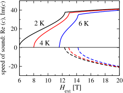
Figure 6: The components of the sound speed $c$ for different temperatures, real for $H_{\rm ext}<H_{\rm ext}^{\rm cr}$, and complex out of this range. Real parts ${\rm Re}(c)$ (solid lines) are positive and ${\rm Im}(c)$ (dashed lines) are negative. Near the threshold ${\rm Im}(c)$ demonstrates to the mean-field square root behavior as discussed below Eq.(103).

5 Conclusions

We investigated macroscopic properties of the triplon condensates taking into account the anomalous density averages. We show that these averages have an important quantitative effect on the specific heat and qualitatively modify the magnetic susceptibility of these systems. The qualitative result of our consideration is related to the dynamical instabilities arising in the condensate. These instabilities are seen as the divergence in the magnetic susceptibility and changes in the sound of the Bogoliubov mode when the external magnetic field becomes stronger than the corresponding temperature-dependent critical value. In this domain, the speed of sound acquires an imaginary part and dependence of its real part on the external field becomes weak, almost flat. These two predictions can easily be verified experimentally in laboratory studies of the static magnetic susceptibility and in the neutron scattering measurements in various magnetic fields.

To conclude this paper, one general comment should be given. Several authors [55, 56] casted doubts on the applicability of the Bose-Einstein condensation approach to magnetic transitions. The irrefutable proof of the validity of this approach can be given by the observation of the Josephson effect, as it was done for magnons in the superfluid He³ [6] and although recently proposed for magnetic insulators [57], not yet observed for the triplon realization. However, we believe that observation of the effects predicted in this paper which are solely based on the improved theory of the Bose-Einstein condensate, will resolve this controversy.

Acknowledgement. AR and SM acknowledge support of the Volkswagen Foundation. This work of EYS was supported by the University of Basque Country UPV/EHU grant GIU07/40, MCI of Spain grant FIS2009-12773-C02-01, and ”Grupos Consolidados UPV/EHU del Gobierno Vasco” grant IT-472-10. We are grateful to H. Kleinert, A. Pelster, M. Modugno, and O. Tchernyshyov for valuable discussions.

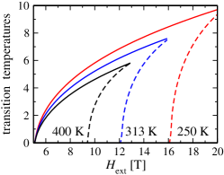
Figure 7: The instability borders (dashed lines) as well as the condensate formation borders (solid lines) for different $U$. With the increase in $U$ the area corresponding to the stable condensate decreases.

References

- [1]
- [2] T. Matsubara and H. Matsuda, Prog. Theor. Phys. 16, 569 (1956); H. Matsuda and T. Tsuneto, ibid 46, 411 (1970).
- [3] M. Tachiki and T. Yamada, J. Phys. Soc. Jpn. 28, 1413 (1970).
- [4] E.G. Batyev and S.L. Braginskii, JETP 60, 781 (1984); E.G. Batyev, ibid 62, 173 (1985).
- [5] For the BEC in magnetic systems under external pumping: V. E. Demidov O. Dzyapko, S. O. Demokritov, G. A. Melkov, and A. N. Slavin, Phys. Rev. Lett. 100, 047205 (2008). For theory: Yu. D. Kalafati and V. L. Safonov, JETP Lett. 50, 149 (1989); I. S. Tupitsyn, P. C. Stamp, and A. L. Burin, Phys. Rev. Lett. 100, 257202 (2008); A. I. Bugrij and V. M. Loktev, Low Temp. Phys. 33, 37 (2007).
- [6] G.E. Volovik, J. Low. Temp. Phys. 153 266 (2008).
- [7] I. Affleck, Phys.Rev B 43, 3215 (1991).
- [8] T. Giamarchi and A. M. Tsvelik, Phys. Rev. B 59, 11398 (1999).
- [9] T. Giamarchi, C. Rüegg, and O. Tchernyshyov, Nature Physics 4, 198 (2008).
- [10] T. Nikuni, M. Oshikawa, A. Oosawa, and H. Tanaka, Phys. Rev. Lett. 84, 5868 (2000).
- [11] A. Oosawa, H. A. Katori, and H. Tanaka, Phys. Rev. B 63, 134416, (2001).
- [12] Ch. C. Rüegg, D. F. McMorrow, B. Normand, H. M. Ronnow, S. E. Sebastian, I. R. Fisher, C. D. Batista, S. N. Gvasaliya, Ch. Niedermayer, and J. Stahn, Phys. Rev. Lett. 98, 017202 (2007).
- [13] M. B. Stone, C. Broholm, D. H. Reich, P. Schiffer, O. Tchernyshyov, P. Vorderwisch, and N. Harrison, New J. Phys. 9, 31 (2007).
- [14] A. A. Aczel, Y. Kohama, M. Jaime, K. Ninios, H. B. Chan, L. Balicas, H. A. Dabkowska, and G. M. Luke, Phys. Rev. B 79, 100409(R) (2009).
- [15] A. Paduan-Filho, K. A. Al-Hassanieh, P. Sengupta, and M. Jaime, Phys. Rev. Lett. 102, 077204 (2009).
- [16] N. Laflorencie and F. Mila, Phys. Rev. Lett. 102, 060602 (2009).
- [17] A. A. Tsirlin and H. Rosner, Phys. Rev. B 83, 064415 (2011).
- [18] T. Dodds, B.-J. Yang, and Y.B. Kim, Phys. Rev. B 81, 054412 (2010).
- [19] J. Sirker, A. Weiße, and O. P. Sushkov, Europhys. Lett. 68, 275 (2004).
- [20] T. D. Stanescu, B. Anderson, and V. Galitski, Phys. Rev. A 78, 023616 (2008).
- [21] M.A. Continentino and A.S. Ferreira, Journal of Magn. and Magn. Mat. 310, 828 (2007).
- [22] E. Ya. Sherman, P. Lemmens, B. Busse, A. Oosawa, and H. Tanaka, Phys. Rev. Lett. 91, 057201 (2003)
- [23] A. Oosawa, K. Kakurai, T. Osakabe, M. Nakamura, M. Takeda and H. Tanaka, J. Phys. Soc. Jpn. 73 1446 (2004).
- [24] Y. Kulik and O. P. Sushkov, arXiv:1104.1245 (unpublished).
- [25] Ch. Rüegg, N. Cavadini, A. Furrer, H.-U. Güdel, K. Krämer, H. Mutka, A. Wildes, K. Habicht, and P. Vorderwisch, Nature 423, 62 (2003).
- [26] A. Rakhimov, E. Ya. Sherman and Chul Koo Kim Phys. Rev. B 81, 020407(R) (2010).
- [27] M. Crisan I. Tifrea, D. Bodea, and I. Grosu, Phys. Rev. B 72, 184414 (2005) provided renormalization group analysis of the triplons BEC.
- [28] V. I. Yukalov, Ann. Phys. 323, 461 (2008)
- [29] G. Misguich and M. Oshikawa, J. Phys. Soc. Jpn. 73, 3429 (2004)
- [30] J. Jensen, Phys. Rev. B 83, 064420 (2011).
- [31] Similar important dispersion-related effects are expected for the Bose-condensation of polaritons: J. Keeling, Phys. Rev. B 74, 155325 (2006).
- [32] F. Yamada, T. Ono, H. Tanaka, G. Misguich, M. Oshikawa, and T. Sakakibara, J. Phys. Soc. Jpn. 77 013701 (2008).
- [33] N.P. Proukakis and B. Jackson, J. Phys. B: At. Mol. Opt. Phys. 41, 203002 (2008).
- [34] H. Kleinert, S. Schmidt, and A. Pelster, Annalen der Physik (Leipzig), 14, 214 (2005).
- [35] Jens O. Andersen, Rev. Mod. Phys. 76, 599 (2004)
- [36] V.I. Yukalov and E.P. Yukalova, Laser Phys. Lett. 2, 506 (2005).
- [37] V. I. Yukalov, A. Rakhimov, and S. Mardonov, Laser Physics 21, 264 (2011).
- [38] H. T. C. Stoof, K. B. Gubbels and D.B.M. Dickerscheid Ultracold Quantum Fields (Springer, 2009)
- [39] A. Rakhimov, Chul-Koo Kim, Sang-Hoon Kim, and Jae-Hyung Yee, Phys. Rev. A 77, 033626 (2008)
- [40] W. H. Dickhoff and D. Van Neck, Many-Body Theory Exposed World Scientific (2005).
- [41] A. Griffin, T. Nikuni, and E. Zaremba, Bose-Condensed Gases at Finite Temperatures Cambridge University Press (2009).
- [42] L. Pitaevskii and S. Stringari, Bose-Einstein Condensation (International Series of Monographs on Physics) Oxford University Press (2003).
- [43] Theory of BEC in ideal relativistic gas was developed in M. Grether, M. de Llano, and G. A. Baker, Jr., Phys. Rev. Lett. 99, 200406 (2007)
- [44] R. Dell’Amore, A. Schilling, and K. Krämer Phys. Rev. B 79, 014438 (2009); R. Dell’Amore, A. Schilling, and K. Krämer, Phys. Rev. B 78, 224403 (2008).
- [45] Kerson Huang, Statistical Mechanics Wiley (1987).
- [46] L.D. Landau and E.M. Lifshitz, Statistical Physics, Course of Theoretical Physics, Volume 5, Butterworth-Heinemann Publ. (1980).
- [47] V. I. Yukalov, Phys. Rev. E 72, 066119 (2005) and references therein.
- [48] D. C. Roberts and M. Ueda, Phys. Rev. A 73, 053611 (2006) perfomed stability analysis for a multicomponent BEC in terms different from those presented here.
- [49] For example, it would be of interest to obtain the neutron scattering measurements data H. Tanaka, A. Oosawa, T. Kato, H. Uekusa, Y. Ohashi, K. Kakurai, and A. Hoser, J. Phys. Soc. Jpn. 70, 939 (2001) for the fields higher than 15 T.
- [50] C.E. Creffield, Phys. Rev. A 79, 063612 (2009).
- [51] M. Modugno, C. Tozzo, and F. Dalfovo, Phys. Rev. A 70, 043625 (2004).
- [52] S. Sinha and Y. Castin, Phys. Rev. Lett. 87, 190402 (2001).
- [53] N. Argaman and Y.B. Band, Phys. Rev. A 83, 023612 (2011), included anomalous density terms in the density functional theory approach.
- [54] Ming-Chiang Chung and A. B. Bhattacherjee, New J. Phys. 11, 123012 (2009).
- [55] D. L. Mills, Phys. Rev. Lett. 98, 039701 (2007).
- [56] V. M. Kalita, I. Ivanova, and V. M. Loktev, Phys. Rev. B 78, 104415 (2008), V. M. Kalita and V. M. Loktev, JETP Letters, 91, 183 (2010), V. M. Kalita and V. M. Loktev, Low Temp. Phys. 36, 665 (2010).
- [57] A. Schilling and H. Grundmann, ArXiv:1101.1811; A. Schilling, H. Grundmann, and R. Dell’Amore, ArXiv:1107.4335.