Crossover between a Short-range and a Long-range Ising model

Abstract

Recently, it has been found that an effective long-range interaction is realized among local bistable variables (spins) in systems where the elastic interaction causes ordering of the spins. In such systems, generally we expect both long-range and short-range interactions to exist. In the short-range Ising model, the correlation length diverges at the critical point. In contrast, in the long-range interacting model the spin configuration is always uniform and the correlation length is zero. As long as a system has non-zero long-range interactions, it shows criticality in the mean-field universality class, and the spin configuration is uniform beyond a certain scale. Here we study the crossover from the pure short-range interacting model to the long-range interacting model. We investigate the infinite-range model (Husimi-Temperley model) as a prototype of this competition, and we study how the critical temperature changes as a function of the strength of the long-range interaction. This model can also be interpreted as an approximation for the Ising model on a small-world network. We derive a formula for the critical temperature as a function of the strength of the long-range interaction. We also propose a scaling form for the spin correlation length at the critical point, which is finite as long as the long-range interaction is included, though it diverges in the limit of the pure short-range model. These properties are confirmed by extensive Monte Carlo simulations.

I introduction

Divergence of the susceptibility is considered one of the characteristics of second-order phase transitions. However, it has been pointed out that in spin-crossover type systems which belong to the mean-field universality class, the spin configuration is uniform even at the critical point. Spin-crossover (SC) materials are molecular crystals, in which the molecules can exist in two different states: the high-spin (HS) state and the low-spin (LS) state. The HS state is preferable at high temperatures because of its high degeneracy, while the LS state is preferable at low temperatures because it has a low enthalpy.SC0 This type of competition exists not only in SC materials, but also in charge-transfer materials, Prussian-blue type materials, Jahn-Teller systems, and martensitic materials. Such systems are generally characterized by the following parameters: the enthalpy difference between the HS and LS states, the difference between their degeneracies (or entropies), and the strength of the intermolecular interactions. A general classification of types of ordering processes in such systems has recently been proposed.Miya0

An important characteristic of this phase transition is an effective long-range interaction caused by an elastic interaction due to the lattice distortion caused by the different sizes of the HS (large) and LS (small) molecules, and the spin configuration at the critical point is uniform with no large-scale clustering.Miya1 It has also been found that the long-range interaction affects dynamical properties.Miya2 ; Mori1 In particular, the critical spinodal phenomena predicted by the mean-field theory are truly realized. This contrasts sharply with the case of short-range models, in which the spinodal phenomena occur as a crossover because nucleation-type fluctuations smear out the criticality.Rikvold

This uniform spin configuration is one of the crucial characteristics of the pure elastic model without short-range interactions. However, in real materials, we expect that both short-range and long-range interactions should exist. For example, if we consider a usual Lennard-Jones potential between molecules which depends on the spin states, the model has both elastic and short-range interactions.Nicolazzi In such systems we expect to see ordering clusters due to the short-range interaction, though the critical phenomena would still be governed by the long-range interaction. Thus, it is an interesting problem to study the crossover between short-range and long-range models.Suzuki In particular, we expect that the correlation length of the spin-correlation function is finite in the thermodynamic limit, even at the critical point, as long as any long-range interaction exists. In the present paper, we study how the critical correlation length increases and ultimately diverges when the long-range interaction vanishes.

To grasp the general features of the competition between the long-range and short-range interactions, in this paper we study a model in which the long-range interactions are those of the Husimi-Temperley model, which is the simplest model in which one can study this effect. We investigate how the spin-correlation function develops due to the short-range interactions. If the long-range interaction is weak, the system shows ordered clusters near the critical point of the short-range model, $T_{\rm c}^{\rm IS}$. If we take the cluster size as the unit length, the model can be regarded as a pure long-range model, and it shows the critical properties of the mean-field universality class at the critical temperature of the model, $T_{\rm c}$ . This picture enables a scaling analysis of the crossover. The difference of the critical temperatures, $T_{\rm c}-T_{\rm c}^{\rm IS}$, is a function of the strength of the long-range interaction. We introduce a formula for the critical temperature as a function of the strength of the long-range interaction, and we perform Monte Carlo simulations to confirm this relation. A model very similar to ours was previously studied by Hastings as a gwell-stirred h approximation for an Ising model on a small-world network.Hast03

A characteristic of the present model is that the correlation length is finite, even at the critical point. We study how the cluster size diverges as the strength of the long-range interaction decreases, and we propose a scaling form for the divergence, which is also confirmed by Monte Carlo simulations.

II Model : Ferromagnetic Ising model with nearest-neighbor and weak infinite-range interactions

II.1 Hamiltonian

First, we consider the effects of a weak, infinitely long-range interaction (Husimi-Temperley model) on the Ising model with ferromagnetic nearest-neighbor interactions on a square lattice,

$${\cal H}_{\rm IS}=-J\sum_{\langle i,j\rangle}\sigma_{i}\sigma_{j},$$ (1)

where $\langle i,j\rangle$ denotes nearest-neighbor pairs, and $\sigma_{i}=\pm 1$ denotes the Ising spin on lattice site $i$. The critical temperature of this modelOnsager is

$$T_{\rm c}^{\rm IS}={2J\over\ln(1+\sqrt{2})}\simeq 2.269\cdots J.$$ (2)

We adopt the following Hamiltonian for the long-range interaction:

$${\cal H}_{\rm HT}=-{4J_{0}\over 2N}\sum_{i=1}^{N}\sum_{j=1}^{N}\sigma_{i}\sigma_{j}.$$ (3)

The critical temperature of this modelHusimi ; Temperley is

$$T_{\rm c}^{\rm HT}=4J_{0}.$$ (4)

With $J_{0}=J$, this critical temperature is equal to that of the mean-field approximation for the Ising model on the present lattice.

For the crossover, we study the following hybrid model,

$${\cal H}=(1-\alpha){\cal H}_{\rm IS}+\alpha{\cal H}_{\rm HT},\quad 0\leq\alpha\leq 1\;.$$ (5)

Here, $\alpha$ controls the relative strength of the long-range interaction.

II.2 Dependence of the critical temperature on $\alpha$

The critical temperature of the model defined by (5) changes from $T_{\rm c}^{\rm IS}$ to $T_{\rm c}^{\rm HT}$ as $\alpha$ changes from 0 to 1. First, we consider the situation in a naive picture. At a temperature $T$, the short-range order is developed by ${\cal H}_{\rm IS}$, and we assume that $N_{\rm cluster}$ spins are tightly correlated and behave as one effective spin. In this case, we introduce an effective spin $\{\tau_{i}\},i=1,\cdots N^{\prime}=N/N_{\rm cluster}$

$$S_{i}=\sum_{j\in{\rm cluster}\;i}^{N_{\rm cluster}}\sigma_{j}=N_{\rm cluster}\tau_{i},\quad\tau_{i}=\pm 1.$$ (6)

Using this effective spin, ${\cal H}_{\rm HT}$ is expressed as

$${\cal H}_{\rm HT}=-{4J_{0}N_{\rm cluster}^{2}\over 2N_{\rm cluster}N^{\prime}}\sum_{i=1}^{N^{\prime}}\sum_{j=1}^{N^{\prime}}\tau_{i}\tau_{j}=-{4J_{0}N_{\rm cluster}\over 2N^{\prime}}\sum_{i=1}^{N^{\prime}}\sum_{j=1}^{N^{\prime}}\tau_{i}\tau_{j}.$$ (7)

The short-range part has contributions from interactions at the interfaces between clusters, and ${\cal H}_{\rm IS}$ is given by

$${\cal H_{\rm IS}}\simeq-{J\sqrt[]{N_{\rm cluster}}}\sum_{\langle i,j\rangle}^{N^{\prime}}\tau_{i}\tau_{j}.$$ (8)

As the clusters grow, the long-range interactions become effectively stronger than the short-range interactions, and the critical temperature is given by

$$T_{\rm c}=4\alpha J_{0}N_{\rm cluster}.$$ (9)

If we estimate $N_{\rm cluster}$ using the Ising correlation length $\xi^{\rm IS}$, which has its origin in the short-range interaction, it can be written as

$$N_{\rm cluster}\simeq(\xi^{\rm IS})^{\gamma\over\nu}=(\xi^{\rm IS})^{2-\eta},$$ (10)

where $\eta$ is the Ising anomalous dimension and the exponent relations are

$$\alpha+2\beta+\gamma=2,$$ (11)

$$\gamma=(2-\eta)\nu,$$ (12)

and $\alpha=0,\beta=1/8,\gamma=7/4,\nu=1,$ and $\eta=1/4$ in the two-dimensional Ising model.exponent Then, using the relation $\xi^{\rm IS}\propto(T-T_{\rm c}^{\rm IS})^{-\nu}$,

$$T_{\rm c}-T_{\rm c}^{\rm IS}\propto\left({4\alpha J_{0}\over T_{\rm c}}\right)^{1\over\gamma}=\left({4\alpha J_{0}\over T_{\rm c}}\right)^{4\over 7}.$$ (13)

In case $\alpha$ is very small, $T_{\rm c}\simeq T_{\rm c}^{\rm IS}$, so

$$T_{\rm c}-T_{\rm c}^{\rm IS}\propto\left({4\alpha J_{0}\over T_{\rm c}^{\rm IS}}\right)^{4\over 7}\propto\alpha^{4\over 7}.$$ (14)

This result agrees with Eq. (9) of Hastings’ paper.Hast03 We can confirm the above picture by an exact argument involving the free energy. Let us consider the free energy of the total system with a fixed magnetization, $m=\sum_{i}\sigma_{i}/N$. The partition function is given explicitly by

$$Z(\beta,m)={\rm Tr}e^{-\beta((1-\alpha){\cal H}_{\rm IS}+\alpha{\cal H}_{\rm HT})}={\rm Tr}e^{-\beta(1-\alpha){\cal H}_{\rm IS}+\beta 4\alpha J_{0}m^{2}N/2}=Z^{\rm IS}(\beta(1-\alpha),m)e^{\beta 4\alpha J_{0}m^{2}N/2},$$ (15)

where $Z^{\rm IS}(\beta,m)$ is the partition function of the Ising model at the inverse temperature $\beta$ for a fixed value of $m$. Therefore, the free energy is given by

$$F(\beta,m)/N=-{1\over\beta N}\ln(Z(\beta,m))=(1-\alpha)f^{\rm IS}(\beta(1-\alpha),m)-4\alpha J_{0}m^{2}/2.$$ (16)

Here $f^{\rm IS}$ is the free energy per spin of the Ising model, and we assume that it can be expanded around the critical point in the following form

$$f^{\rm IS}(\beta(1-\alpha),m)\simeq{1\over 2\chi^{\rm IS}(\beta(1-\alpha))}m^{2}+\cdots.$$ (17)

Thus the critical point of the present model is given by ${\partial^{2}F(\beta_{\rm c},m)\over\partial m^{2}}|_{m=0}=0$, or

$${(1-\alpha)\over\chi^{\rm IS}(\beta_{\rm c}(1-\alpha))}-{4\alpha J_{0}}=0,$$ (18)

where the susceptibility of the hybrid model (5) diverges. If we adopt the relation

$$\chi^{\rm IS}(T)\propto(T-T_{\rm c}^{\rm IS})^{-\gamma},$$ (19)

the critical point is given by

$$T_{\rm c}-(1-\alpha)T_{\rm c}^{\rm IS}\propto(4\alpha J_{0})^{1\over\gamma}(1-\alpha)^{1-{1\over\gamma}}\simeq\alpha^{1\over\gamma}$$ (20)

which agrees with (14) for small $\alpha$. We note that equation (19) holds only when $T$ is very close to $T_{\rm c}^{\rm IS}$, so equation (20) holds only when $T_{\rm c}$ is very close to $(1-\alpha)T_{\rm c}^{\rm IS}$. Namely, equation (20) is only valid for $\alpha\ll 1$.

For $\alpha=1$,

$$\lim_{\alpha\rightarrow 1}F(\beta,m)/N=\lim_{\alpha\rightarrow 1}(1-\alpha)f^{\rm IS}(\beta(1-\alpha),m)-4\alpha J_{0}m^{2}/2={T\over 2}m^{2}-4J_{0}m^{2}/2+\cdots\quad.$$ (21)

In this case (18) yields $T_{c}=4J_{0}$, the critical temperature of the Husimi-Temperly model (4).

To obtain the numerically correct amplitude for $T_{\rm c}(\alpha)$, we need the Ising susceptibility near the critical point for $T>T_{\rm c}^{\rm IS}$,ising_sus

$$\chi^{\rm IS}(\beta)=\beta C_{\rm 0}\left({1\over\tilde{t}}\right)^{\gamma},\hskip 14.22636pt\gamma=7/4$$ (22)

with $C_{\rm 0}=0.962582\cdots$, and

$$\tilde{t}={T-T_{\rm c}^{\rm IS}\over T}={T_{\rm c}^{\rm IS}\over T}t.$$ (23)

Equation (18) can be written as

$${T_{\rm c}\over C_{\rm 0}}\left({(1-\alpha)T_{\rm c}^{\rm IS}\over T_{\rm c}}\right)^{7\over 4}\left({T_{\rm c}-(1-\alpha)T_{\rm c}^{\rm IS}\over(1-\alpha)T_{\rm c}^{\rm IS}}\right)^{7\over 4}=4\alpha J_{0}.$$ (24)

We write $t_{\rm c}(\alpha)={T_{\rm c}-T_{\rm c}^{\rm IS}\over T_{\rm c}^{\rm IS}}$, so

$$(1+t_{\rm c})^{4\over 7}(t_{\rm c}+\alpha)=(1+t_{\rm c})\left({4\alpha J_{0}C_{0}\over T_{\rm c}^{\rm IS}}\right)^{4\over 7}.$$ (25)

Expanding to lowest order in $t_{\rm c}$ and $\alpha$ while setting $J_{0}=J$, we get

$$t_{\rm c}\simeq A\alpha^{4\over 7}\hskip 7.11317pt{\rm with}\hskip 7.11317ptA=\left({4J_{0}C_{0}\over T_{\rm c}^{\rm IS}}\right)^{4\over 7}\simeq 1.352745,$$ (26)

or equivalently,

$${T_{\rm c}(\alpha)-T_{\rm c}^{\rm IS}\over T_{\rm c}^{\rm MF}-T_{\rm c}^{\rm IS}}\simeq 1.773517\alpha^{4\over 7}.$$ (27)

This result agrees with (14).

II.3 Monte Carlo study of the $\alpha$ dependence of $T_{\rm c}$

In order to confirm the scaling relation of the previous subsection, we estimated the critical temperatures for various values of $\alpha$ by Monte Carlo simulations. Here we fixed both $J$ and $J_{0}$ to 1.0. Therefore, $T_{c}^{\rm IS}=2.269\cdots$ and $T_{c}^{\rm HT}=4$ in these units. We used a standard Metropolis method, adopting periodic boundary conditions. In most cases, we performed 500,000 MCS (Monte Carlo steps) for the data with 100,000 MCS for the equilibration. From now on, $L$ denotes the linear system size in units of the lattice constant, so the total number of spins is $L^{2}$.

We estimate a candidate for the critical temperature $T_{\rm c}(\alpha)$ for each value of $\alpha$. In order to obtain this value, we study the size dependence of the peak position of the so-called absolute susceptibilityLandau

$$\tilde{\chi}\equiv{1\over N}(\langle M^{2}\rangle-\langle|M|\rangle^{2})$$ (28)

as a ‘critical point’ $T_{\rm c}(\alpha,L)$ for the size $L$. We expect that the peak position saturates at the critical temperature in the thermodynamic limit:

$$T_{\rm c}(\alpha,L)\rightarrow T_{\rm c}(\alpha,\infty).$$ (29)

In Fig. 1, we depict a typical size dependence of the peak for $\alpha=0.001$.

Figure 1: (Color online) Temperature dependences of $\tilde{\chi}$ for $\alpha=0.001$ and $L=20,40,80,160,$ and $320$ from below to above. The peak positions are marked by circles. For large systems, they increase with increasing $L$. The left vertical dashed line represents the critical temperature for the pure Ising model, and the right-hand line represents the critical temperature for $\alpha=0.001$ obtained by the Binder cumulant method (see below).

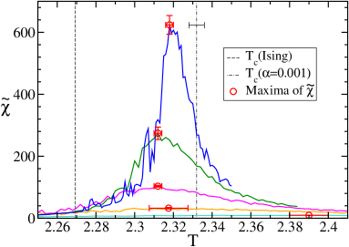
By a general argument we expect the following size dependence:

$$T_{\rm c}(\alpha,L)-T_{\rm c}(\alpha,\infty)\propto L^{-1/\nu}.$$ (30)

Here, $\nu$ is the critical exponent of the correlation length. However, in the present case, the critical phenomena belong to the mean-field universality class, and the definition of $\nu$ is subtle. Namely, if we consider the spatial correlation of the Gaussian model, $\nu=1/2$, while in the scaling relation in the mean-field universality class, we have the effective $\nu=2/d$.Miya1 ; privman ; Luijten1 In the infinite-range (HT) model, distances are not well defined, and only the total number of spins, $N$, has a meaning. Thus, we should rewrite the relation (30) as

$$T_{\rm c}(\alpha,L)-T_{\rm c}(\alpha,\infty)\propto N^{-1/d\nu},$$ (31)

where we take the latter case ($\nu=2/d$) as we did in a previous paper.Miya1 In the present case $d=2$ and thus $N=L^{2}$, which gives

$$\nu_{\rm HT}=1,$$ (32)

which accidentally agrees with that of the short-range Ising model,

$$\nu_{\rm IS}=1.$$ (33)

In Fig. 2, we plot the peak position of $\tilde{\chi}$ by open squares as a function of $L^{-1}$ for several values of $\alpha$. The critical temperature $T_{\rm c}(\alpha,\infty)$ could in principle be estimated by linear extrapolation in $L^{-1}$.

Figure 2: (Color online) Estimates for $T_{\rm c}(\alpha,L)$ for different values of $\alpha$ vs $L^{-1}$. $\alpha=0$ (pure Ising), $0.0001,0.001,0.01,0.1,0.5,$ and $1$ (Husimi-Temperley) from below to above. $L=20,40,80,160,$ and $320$. The squares denote the peak positions of $\tilde{\chi}$, and the circles denote the crossing positions of the Binder cumulant for $L$ and $L/2$. The upper and lower dashed lines mark the exact critical temperatures for the HT and Ising models, respectively. The inset shows detail for $\alpha=0.001,0.0001,$ and $0$ (pure Ising).

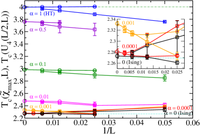However, we find a non-monotonic dependence of the peak position as a function of $L^{-1}$ for small values of $\alpha$. (See also Fig. 1.) Only when the size becomes large enough to show the critical behavior of the HT model, can we apply the scaling relation (30). For small sizes, the system behaves like a short-range model, and the peak position moves differently. Indeed, we find that in the scaling region, the peak position approaches $T_{c}(\alpha,\infty)$ from below. However, for $\alpha\leq 0.01$ we find that it decreases with $L$ for small values of $L$. For $\alpha=0.001$, we find that the peak position finally increases again when $L$ goes from $160$ to $320$, while for $\alpha=0.0001$, it continues to decrease for all values of $L$ considered. Thus, we cannot estimate the infinite-system value by a simple extrapolation of the peak position in $L^{-1}$ for $\alpha=0.0001$.

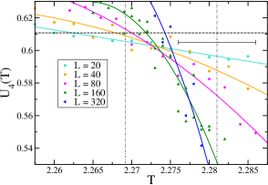
To obtain more accurate estimates for small $\alpha$, we also estimated $T_{c}(\alpha,L)$ from the crossing point of the fourth-order Binder cumulant,bindercumulant

$$U_{4}(\alpha,L)=1-{\langle m^{4}\rangle\over 3\langle m^{2}\rangle^{2}},$$ (34)

for $L$ and $L/2$. When $L$ and $\alpha$ are small, the crossing value of $U_{4}(\alpha,L)$ is near the Ising fixed-point value, $U_{4}^{*\rm IS}\simeq 0.61...$,IsingCum while for larger $L$ and/or $\alpha$, the crossing moves down toward the exact value for the HT model, $U_{4}^{*\rm HT}=1-\Gamma^{4}(1/4)/24\pi^{2}=0.27...$,Brezin ; Luijten where $\Gamma(x)$ is the Gamma function. The values of $T$ at the crossing points are shown as circles vs $L^{-1}$ for different values of $\alpha$ in Fig. 2. The temperature dependences of $U_{4}(\alpha,L)$ for different $\alpha$ and $L$ are shown in Fig. 3. For $\alpha=0.1$, we find the crossing points located near $U_{4}^{*\rm HT}$, indicating that the critical properties belong to the mean-field universality class. For $\alpha=0.01$ and 0.001, we find that the crossing points move from near $U_{4}^{*\rm IS}$ toward $U_{4}^{*\rm HT}$ as $L$ increases. These results indicate that the critical point of the hybrid model belongs to the mean-field universality class for all $\alpha>0$. In the case of $\alpha=0.0001$, the crossing point of the Binder cumulants for $(L,L/2)=(320,160)$ is still near $U_{4}^{*\rm IS}$. Because we assume that the critical behavior for nonzero $\alpha$ belongs to the mean-field universality class, we get a series of upper bounds on the critical temperature as the temperature at which $U_{4}(\alpha,L)$ crosses $U_{4}^{\rm HT}$. Lower bounds are given by the cumulant-crossing temperatures. Our best estimates for $T_{c}$ are obtained by linearly extrapolating the crossing temperatures to $L^{-1}=0$ . In this way, we estimated the $T_{\rm c}(\alpha=0.0001)=2.281\pm 0.005$. In Appendix A we show in detail how we estimated this value.

$$\begin{array}[]{cc}\includegraphics[scale={0.3}]{03Mixed01Mlongrun_Bx_detail_2_v2.eps}&\includegraphics[scale={0.3}]{04Mixed001Mlongrun_Bx_detail_2_v2.eps}\\ ({\rm a})&({\rm b})\\ \\ \includegraphics[scale={0.3}]{05Mixed0001Mlongrun_Bx_detail_v2.eps}&\includegraphics[scale={0.3}]{06Mixed00001Mlongrun_Bx_detail_v2.eps}\\ ({\rm c})&({\rm d})\end{array}$$

Figure 3: (Color online) Temperature dependence of the Binder cumulant for (a) $\alpha=0.1$, (b) $\alpha=0.01$, (c) $\alpha=0.001$, and (d) $\alpha=0.0001$. Points are Monte Carlo data, and the solid lines are polynomial fits. The upper and lower horizontal lines are the fixed-point values for the Ising model and the Husimi-Temperley model respectively, and the left vertical lines in (c) and (d) represent the critical temperature of the pure Ising model. The vertical dashed lines with horizontal error bars represent the critical temperatures obtained by extrapolation of the crossing temperatures as described in Appendix A.

The extrapolated values for $T_{c}(\alpha,\infty)-T_{\rm c}^{\rm IS}$ are shown on a log-log scale in Fig. 4. For small $\alpha$, the data points fall on a straight line of slope ${4/7}$. As mentioned above, to obtain more accurate estimates of the critical temperatures from $\tilde{\chi}$, we would need to perform MC with much larger systems. For small $\alpha$, the results from the Binder cumulants are in good agreement with the power law, $T_{\rm c}(\alpha)-T_{\rm c}^{\rm IS}\propto\alpha^{4/7}$.

Figure 4: (Color online) The $\alpha$ dependence of the normalized critical-temperature difference, $[T_{\rm c}(\alpha)-T_{\rm c}^{\rm IS}]/[T_{\rm c}^{\rm HT}-T_{\rm c}^{\rm IS}]$ in a log-log plot. The circles and triangles (red online) denote critical temperatures obtained from the peak position of $\tilde{\chi}$ for $L=320$ and $80$ respectively, and the squares (blue online) denote critical temperatures obtained from Binder cumulants. The horizontal dashed line (red online) represents $y=1$, and the oblique dashed line (blue online) represents the numerically exact theoretical estimate, $1.773517\alpha^{4/7}$ (27). The latter line, which involves no adjustable parameters, agrees very well with the cumulant-generated data for small $\alpha$.

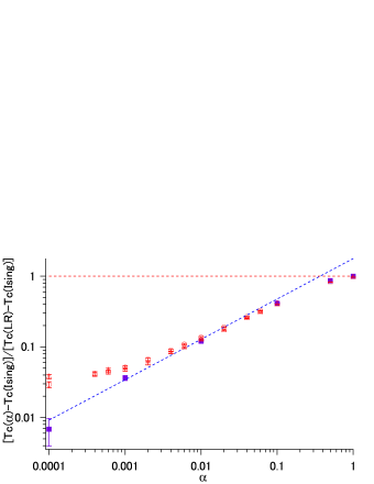Thus, we confirm the scaling relation (13):

$$T_{c}(\alpha,\infty)-T_{c}(0,\infty)\propto\alpha^{1/\gamma_{\rm IS}}.$$ (35)

III Cluster size at the critical point

In the pure long-range model, all spins interact with each other. Thus, the concept of distance has no meaning, and the system does not show any clustering. On the other hand, in the short-range model, the ordering process occurs as a development of short-range order, and the cluster size, i.e., the correlation length, represents the extent of the ordering. In Fig. 5(a) and Fig. 5(b), we depict typical spin configurations at the critical temperature $T_{\rm c}(\alpha)$ of the short-range model and the long-range model, respectively. A clear difference between the two cases is evident.

$$\begin{array}[]{cc}\includegraphics[scale={0.4}]{08ising.eps}&\includegraphics[scale={0.4}]{09husimi1.eps}\\ ({\rm a})&({\rm b})\end{array}$$

Figure 5: (Color online) (a) Spin configurations for Ising model at $T_{\rm c}^{\rm IS}=2.269J$, $L=100$ and (b) Husimi-Temperley model at $T_{\rm c}^{\rm HT}=4J_{0}$.

Here it should be noted that non-divergence of the correlation length does not mean non-divergence of the susceptibility. In the mean-field model, the susceptibility diverges as $|T-T_{\rm c}^{\rm HT}|^{-1}$. This means that the fluctuation of the magnetization $M$ diverges as

$${1\over N}(\langle M^{2}\rangle-\langle M\rangle^{2})\propto|T-T_{\rm c}^{\rm HT}|^{-1}.$$ (36)

This fluctuation can be observed as the fluctuation of the uniform density of the spin configuration. In Fig. 6 we depict typical configurations at $T_{\rm c}^{\rm HT}$ with different $M/N=m$. We note that the spin configurations are uniform, but the ratio of numbers of up and down spins fluctuates. This causes large fluctuations in the magnetization $M$, but not in the cluster size. In the long-range model, large numbers of spins change uniformly.

$$\begin{array}[]{ccc}\includegraphics[scale={0.3}]{10husimi2.eps}&\includegraphics[scale={0.3}]{09husimi1.eps}&\includegraphics[scale={0.3}]{11husimi3.eps}\\ ({\rm a})&({\rm b})&({\rm c})\end{array}$$

Figure 6: (Color online) Spin configurations for the Husimi-Temperley model for (a)$\langle m\rangle$ $\simeq$ 0.3 at $T_{\rm c}^{\rm HT}$, (b)$\langle m\rangle$ $\simeq$ 0.0 at $T_{\rm c}^{\rm HT}$ and (c) $\langle m\rangle$ $\simeq$ -0.3 at $T_{\rm c}^{\rm HT}$.

In the hybrid model (5), the criticality belongs to the mean-field universality class. However, short-range order also develops. Thus, we expect a finite correlation length at the critical point, which increases as $\alpha$ decreases. In Fig. 7, we depict typical configurations at the critical temperature for various values of $\alpha$. We clearly see that the size of the clusters increases with decreasing $\alpha$.

$$\begin{array}[]{cc}\includegraphics[scale={0.3}]{12snap00001_tc.eps}&\includegraphics[scale={0.3}]{13snap0001_tc.eps}\\ ({\rm a})&({\rm b})\\ \includegraphics[scale={0.3}]{14snap001_tc.eps}&\includegraphics[scale={0.3}]{15snap01_tc.eps}\\ ({\rm c})&({\rm d})\end{array}$$

Figure 7: (Color online) Typical configurations of the hybrid model at the critical temperature $T_{\rm c}(\alpha)$ for (a) $\alpha=0.0001$, (b) $\alpha=0.001$, (c) $\alpha=0.01$, and (d) $\alpha=0.1$.

IV Finite-size scaling of the cluster size at the critical point

IV.1 Scaling function

In this section, we study the correlation length at the critical point for several values of $\alpha$. From the relation (20), we expect the following relation between the correlation length $\xi_{\rm c}$ at the critical temperature and $\alpha$ :

$$\xi_{\rm c}(\alpha)\propto(T_{\rm c}-(1-\alpha)T_{\rm c}^{\rm IS})^{-\nu_{\rm IS}}\simeq\left((4\alpha J_{0}\chi_{0})^{1/\gamma_{\rm IS}}\right)^{-\nu_{\rm IS}}\propto\alpha^{-\nu_{\rm IS}/\gamma_{\rm IS}}$$ (37)

for $\alpha\ll 1$. Moreover, for $\alpha\ll 1$ we may assume the following finite-size scaling relation with the linear dimension of the system $L$

$$\xi_{\rm c}(\alpha,L)=Lf\left(L\alpha^{\nu\over\gamma}\right)=Lf\left(L\alpha^{4\over 7}\right),$$ (38)

where $f(x)$ is a scaling function which is proportional to $1/x$ for large $x$, and constant for small $x$.

In the case of the short-range Ising model, we can estimate the divergence of the correlation length by making use of the susceptibility:

$$\chi={1\over Nk_{\rm B}T}\sum_{i,j}\langle\sigma_{i}\sigma_{j}\rangle\sim{1\over k_{\rm B}T}\int_{0}^{L}{1\over r^{d-2+\eta}}e^{-r/\xi}dr\sim\xi^{2-\eta}=\xi^{\gamma\over\nu}.$$ (39)

However, in the present long-range interaction model, the value of the magnetization fluctuates uniformly but not spatially. Therefore, we cannot estimate $\xi$ from $\chi$.

IV.2 Measurement of $\xi$ at $T_{\rm c}$ : Direct measurement of the correlation function

Here we estimate the correlation length from the spin correlation function $c(r)=\langle\sigma_{i}\sigma_{j}\rangle$, where $r$ is the distance between the sites $i$ and $j$, by the following definition

$$\xi(L)={\int_{0}^{L/2}\left(c(r)-c(L/2)\right)rdr\over\int_{0}^{L/2}\left(c(r)-c(L/2)\right)dr}.$$ (40)

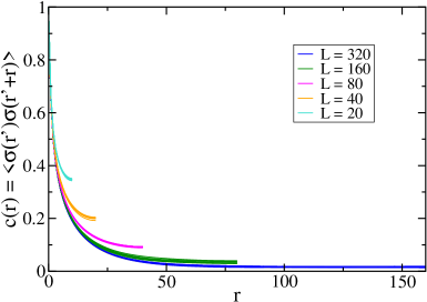
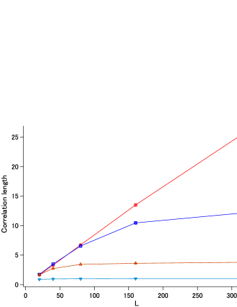
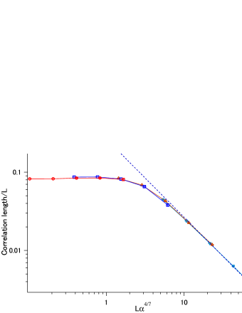
This definition gives the correlation length if $c(r)$ decays exponentially to its large-$r$ value, and also for general cases it gives an estimate of the correlation length. In Fig. 8, we depict a typical example of $c(r)$. At large distance, $c(r)$ is constant,Miya1 proportional to $\sqrt[]{N}$. The size dependence of $\xi(\alpha,L)$ is depicted in Fig. 9, where we confirm that the correlation length saturates for large $L$ as expected, even for quite small values of $\alpha$. The estimated $\xi(\alpha,L)$ are plotted in the finite-size scaling plot Fig. 10, in which we assume $\xi$ at the critical point depends on $\alpha$ as (38). We find that the data collapse onto a scaling function and thereby confirm the theoretical scaling relation (38).

Figure 8: (Color online) The disconnected spin correlation function $c(r)$ at the critical point $T_{\rm c}(\alpha)=2.332$ for $\alpha=0.001$. For each value of $L$, the results of seven independent runs of $10^{6}$ MCS each are shown.

Figure 9: (Color online) The size dependence of the correlation length at the critical point $T_{\rm c}(\alpha)$. Circles, squares, up-triangles, and down-triangles represent $T=2.281$ for $\alpha=0.0001$, $T=2.332$ for $\alpha=0.001$, $T=2.477$ for $\alpha=0.01$ and $T=2.984$ for $\alpha=0.1$, respectively.

Figure 10: (Color online) The scaling plot of the correlation length at the critical point. Circles, squares, up-triangles, and down-triangles represent $T=2.281$ for $\alpha=0.0001$, $T=2.332$ for $\alpha=0.001$, $T=2.477$ for $\alpha=0.01$ and $T=2.984$ for $\alpha=0.1$, respectively. The linear system sizes are $L=20,40,80,160,$ and $320$. The dashed line is proportional to $y=1/x$. The data are in excellent agreement with the scaling relation (38).

V Summary

We found that in systems with both long and short-range interactions, the long-range interaction dominates the critical properties, even if it is infinitely weak. At the critical temperature, although the susceptibility diverges, the cluster size does not. At the critical temperature, the system has a finite correlation length.

In this paper, we obtained a formula for the change of the critical temperature as a function of the strength $\alpha$ of the long-range interaction, and also a scaling form for the spin correlation length at the critical point.

The crossover of the nature of the order as the length scale changes was studied by a Monte Carlo method. We investigated the values of the Binder cumulant at its crossing points. It moved from the value of the short-range Ising model to that of the mean-field universality class, which enabled us to estimate the critical point systematically. The result agrees well with our proposed formula. We further note that our model can be considered as a gwell-stirred h approximation for the Ising model on a small-world network.Hast03

We also proposed a scaling relation for the correlation length at the critical point as a function of $\alpha$. At the critical point, the spin correlation function at large distances is constant,Miya1 proportional to $\sqrt[]{N}$ with a short-range component characteristic of the correlation length $\xi$. We obtained the value of the correlation length from the simulated spin correlation function, thus providing numerical confirmation of our proposed a scaling function.

We expect that the results found in this paper are applicable also for real system with degrees of freedom corresponding to lattice deformation. A study of such a model will be published elsewhere.Next We hope this kind of phenomena will be found in future experiments.

Appendix A The estimation of $T_{c}(\alpha)$ from the crossing points of the Binder cumulant

In the present models, the system behaves like a short-range Ising model for small $\alpha$ and $L$. If we study the crossing point of the Binder cumulants, $U_{4}(\alpha,L)$, for small values of $L$ and at small $\alpha$, the crossing point gives a value close to that of the Ising model, i.e., $U_{4}^{*\rm IS}\simeq 0.61\dots$. However, as the size increases, the crossing points approach the fixed-point value of the mean-field model, $U_{4}^{*\rm HT}\simeq 0.27\dots$. For $\alpha=0.0001$, the crossing point of the two largest sizes simulated, $L=320$ and $160$, still stays near $0.57$, which is far from $U_{4}^{*\rm HT}$. Thus, we cannot obtain the critical temperature directly. Here we estimate $T_{c}(\alpha=0.0001)$ in the following way. We obtain the crossing points for systems with $L$ and $L^{\prime}=L/2$ as depicted in Fig. 11. Continuous lines for the cumulants as functions of $T$ were obtained as polynomial fits to densely spaced Monte Carlo data obtained from simulation runs of up to $10^{7}$ MCS. We assume the following properties: (1) $U_{4}$ at the crossing point for large $L$ equals $U_{4}^{*\rm HT}$, (2) $U_{4}(\alpha,L)$ is a monotonic function of the temperature, and (3) the crossing temperature increases monotonically with $L$. From these assumptions we find in Fig. 11 that $T_{c}(\alpha)$ is above $T=2.277$ which is the crossing temperature for $L^{\prime}=160$ and $L=320$. Because $U_{4}(\alpha,L=320)$ crosses $U_{4}^{*\rm HT}$ at $T=2.289$, $T_{c}(\alpha)$ is below $T=2.289$. By linear extrapolation with respect to $1/L$ of the crossing values for $L^{\prime}/L=80/160$ and $160/320$ (see the inset in Fig. 2), we estimated the critical temperature as

$$T_{c}(\alpha=0.0001)=2.281\pm 0.005.$$ (41)

Figure 11: Detail of the crossings of the Binder cumulant for $\alpha=0.0001$. This figure is a magnified portion of Fig. 3(d).

References

- (1) P. Gütlich and H. E. Goodwin, Editors, Spin Crossover in Transition Metal Compounds I, II, and III, Topics in Current Chemistry Vols. 233, 234, 235 (Springer-Verlag, Berlin Heidelberg New York, 2004).
- (2) S. Miyashita, Y. Konishi, H. Tokoro, M. Nishino, K. Boukheddaden, and F. Varret, Prog. Theor. Phys. 114, 719 (2005).
- (3) S. Miyashita, Y. Konishi, M. Nishino, H. Tokoro, and P. A. Rikvold, Phys. Rev. B 77, 014105 (2008).
- (4) M. Nishino, K. Boukheddaden, Y. Konishi, and S. Miyashita, Phys. Rev. Lett. 98, 247203 (2007).
- (5) C. Enachescu, L. Stoleriu, A. Stancu, and A. Hauser, Phys. Rev. Lett. 102, 2572044 (2009).
- (6) M. Nishino, C. Enachescu, S. Miyashita, K. Boukheddaden, and F. Varret, Phys. Rev. B 82, R020409 (2010).
- (7) Y. Konishi, H. Tokoro, M. Nishino, and S. Miyashita, Phys. Rev. Lett. 100, 067206 (2008).
- (8) S. Miyashita, P. A. Rikvold, T. Mori, Y. Konishi, M. Nishino, and H. Tokoro, Phys. Rev. B 80, 064414, (2009).
- (9) T. Mori, S. Miyashita, and P. A. Rikvold, Phys. Rev. E 81, 011135 (2010).
- (10) P. A. Rikvold, H. Tomita, S. Miyashita and S. W. Sides, Phys. Rev. E 49, 5080 (1994).
- (11) W. Nicolazzi, S. Pillet, and C. Lecomte, Phys. Rev. B 78, 174401 (2008).
- (12) M. Suzuki, J. Phys. Soc. Jpn. 21, 2140 (1966).
- (13) M. B. Hastings, Phys. Rev. Lett. 91, 098701 (2003).
- (14) L. Onsager, Phys. Rev. 65, 117 (1944).
- (15) K. Husimi, Lecture at the meeting of Phys. Soc. Jpn., May (1953).
- (16) H. N. V. Temperley, Proc. Phys. Soc. 67 (1954).
- (17) C. Itzykson and J.M. Drouffe, Statistical field theory: 1 and 2 (Cambgridge, 1989).
- (18) W. P. Orrick, B. Nickel, A. J. Guttmann and J. H. H. Perk, J. Stat. Phys. 102, 795, (2001).
- (19) A. M. Ferrenberg and D. P. Landau, Phys. Rev. B 44, 105081 (1991).
- (20) V. Privman and M. E. Fisher, J. Stat. Phys. 33, 385 (1983).
- (21) E. Luijiten and H. W. J. Blöte, Phys. Rev. B 56, 8945 (1997), and references therein.
- (22) K. Binder, Phys. Rev. Lett. 47, 693 (1981).
- (23) G. Kamieniarz and H. W. J. Blöte, J. Phys. A 26, 201 (1993).
- (24) E. Brezin and J. Zinn-Justin, Nucl. Phys. B 257, 867 (1985).
- (25) E. Luijten and H. W. J. Blöte, Int. J. Mod. Phys. C 6, 359 (1995).
- (26) T. Nakada, T. Mori, M. Nishino, S. Miyashita, S. Todo, W. Nicollazzi, and P. A. Rikvold, in preparation.