The cohomology ring of the GKM graph
of a flag manifold of classical type

Abstract.

If a closed smooth manifold $M$ with an action of a torus $T$ satisfies certain conditions, then a labeled graph $\mathcal{G}_{M}$ with labeling in $H^{2}(BT)$ is associated with $M$, which encodes a lot of geometrical information on $M$. For instance, the “graph cohomology” ring $H_{T}^{*}(\mathcal{G}_{M})$ of $\mathcal{G}_{M}$ is defined to be a subring of $\bigoplus_{v\in V(\mathcal{G}_{M})}H^{*}(BT)$, where $V(\mathcal{G}_{M})$ is the set of vertices of $\mathcal{G}_{M}$, and is known to be often isomorphic to the equivariant cohomology $H^{*}_{T}(M)$ of $M$. In this paper, we determine the ring structure of $H_{T}^{*}(\mathcal{G}_{M})$ with $\mathbb{Z}$ (resp. $\mathbb{Z}[\frac{1}{2}]$) coefficients when $M$ is a flag manifold of type A, B or D (resp. C) in an elementary way.

1. Introduction

Let $T$ be a compact torus of dimension $n$ and $M$ a closed smooth $T$-manifold. The equivariant cohomology of $M$ is defined to be the ordinary cohomology of the Borel construction of $M$, that is,

$$H^{*}_{T}(M):=H^{*}(ET\times_{T}M)$$

where $ET$ denotes the total space of the universal principal $T$-bundle $ET\to BT$ and $ET\times_{T}M$ denotes the orbit space of $ET\times M$ by the diagonal $T$-action. Throughout this paper, all cohomology groups are taken with $\mathbb{Z}$ coefficients unless otherwise stated. The equivariant cohomology of $M$ contains a lot of geometrical information on $M$. Moreover it is often easier to compute $H^{*}_{T}(M)$ than $H^{*}(M)$ by virtue of the Localization Theorem which implies that the restriction map

(1.1) $$\iota^{*}\colon H^{*}_{T}(M)\to H^{*}_{T}(M^{T})$$

to the $T$-fixed point set $M^{T}$ is often injective, in fact, this is the case when $H^{odd}(M)=0$. When $M^{T}$ is isolated, $H^{*}_{T}(M^{T})=\bigoplus_{p\in M^{T}}H^{*}_{T}(p)$ and hence $H^{*}_{T}(M^{T})$ is a direct sum of copies of a polynomial ring in $n$ variables because $H^{*}_{T}(p)=H^{*}(BT)$.

Therefore we suppose that $H^{odd}(M)=0$ and $M^{T}$ is isolated. Goresky-Kottwitz-MacPherson [5] (see also [6, Chapter 11]) found that under the further condition that the weights at a tangential $T$-module are pairwise linearly independent at each $p\in M^{T}$, the image of $\iota^{*}$ in (1.1) above is determined by the fixed point sets of codimension one subtori of $T$ when considering cohomology with $\mathbb{Q}$ coefficients. Their result motivated Guillemin-Zara [7] to associate a labeled graph $\mathcal{G}_{M}$ with $M$ and define the “graph cohomology” ring $H_{T}^{*}(\mathcal{G}_{M})$ of $\mathcal{G}_{M}$, which is a subring of $\bigoplus_{p\in M^{T}}H^{*}(BT)$. Then the result of Goresky-Kottwitz-MacPherson can be stated that $H^{*}_{T}(M)\otimes\mathbb{Q}$ is isomorphic to $H_{T}^{*}(\mathcal{G}_{M})\otimes\mathbb{Q}$ as graded rings when $M$ satisfies the conditions mentioned above.

The result of Goresky-Kottwitz-MacPherson can be applied to many important $T$-manifolds $M$ such as flag manifolds, compact smooth toric varieties and so on. When $M$ is such a nice manifold, $H^{*}_{T}(M)$ is known to be often isomorphic to $H_{T}^{*}(\mathcal{G}_{M})$ without tensoring with $\mathbb{Q}$ (see [9], [10] for example). In this paper, we determine the ring structure of $H_{T}^{*}(\mathcal{G}_{M})$ (resp. $H_{T}^{*}(\mathcal{G}_{M})\otimes\mathbb{Z}[\frac{1}{2}]$) in an elementary way when $M$ is a flag manifold of type A, B or D (resp. C).

The equivariant cohomology ring $H^{*}_{T}(M)$ of a flag manifold $M$ of classical type is determined (see [4] for example) and our computation of $H^{*}_{T}(\mathcal{G}_{M})$ confirms that (resp. $H^{*}_{T}(M)\otimes\mathbb{Z}[\frac{1}{2}]$) is isomorphic to $H_{T}^{*}(\mathcal{G}_{M})$ (resp. $H_{T}^{*}(\mathcal{G}_{M})\otimes\mathbb{Z}[\frac{1}{2}]$) when $M$ is of type A, B or D (resp. C). The main point in our computation is to show that $H_{T}^{*}(\mathcal{G}_{M})$ is generated by some elements which have a simple combinatorial description. When $M$ is a flag manifold of type $A_{n-1}$, those elements $\tau_{1},\dots,\tau_{n}$ in $H_{T}^{*}(\mathcal{G}_{M})$ correspond to the equivariant first Chern classes in $H^{*}_{T}(M)$ of complex line bundles over $M$ obtained from the flags. One can show that those first Chern classes generate $H^{*}_{T}(M)$ over $H^{*}(BT)$ using topological techniques. However, our concern is to compute the graph cohomology $H_{T}^{*}(\mathcal{G}_{M})$ directly, and so we show that $\tau_{1},\dots,\tau_{n}$ generate $H_{T}^{*}(\mathcal{G}_{M})$ over $H^{*}(BT)$ in a purely combinatorial or elementary way.

This paper is organized as follows. In Section 2 we introduce the notion of a labeled graph and its graph cohomology following the notion of GKM graph and its graph cohomology. We treat type A in Section 3, which is a prototype of our argument. Type C is treated in Section 4 and the argument is almost the same as type A if we work over $\mathbb{Z}[\frac{1}{2}]$ coefficients. Types B and D can also be treated similarly but more subtle arguments are necessary when we work over $\mathbb{Z}$ coefficients. This is done in Sections 5 and 6.

This paper is the detailed and improved version of the announcement [1]. Recently the first author ([2]) has determined the ring structure of $H^{*}_{T}(\mathcal{G}_{M})$ along the line developed in this paper when $M$ is the flag manifold of type $G_{2}$.

2. Labeled graphs and graph cohomology

Let $T$ be a compact torus of dimension $n$. Any homomorphism $f$ from $T$ to a circle group $S^{1}$ induces a homomorphism $f^{*}\colon H^{*}(BS^{1})\to H^{*}(BT)$, so assigning $f$ to $f^{*}(u)$, where $u$ is a fixed generator of $H^{2}(BS^{1})$, defines a homomorphism from $\operatorname{Hom}(T,S^{1})$ (the group of homomorphisms from $T$ to $S^{1}$) to $H^{2}(BT)$. As is well-known, this homomorphism is an isomorphism so that we make the following identification

$$\operatorname{Hom}(T,S^{1})=H^{2}(BT)$$

and use $H^{2}(BT)$ instead of $\operatorname{Hom}(T,S^{1})$ throughout this paper.

Let $\mathcal{G}$ be a graph with labeling

$$\ell(e)\in H^{2}(BT)\quad\text{for each edge $e$ of $\mathcal{G}$.}$$

We call $\mathcal{G}$ a labeled graph in this paper. Remember that $H^{*}(BT)$ is a polynomial ring over $\mathbb{Z}$ generated by elements in $H^{2}(BT)$.

Definition.

The graph cohomology ring of $\mathcal{G}$, denoted $H_{T}^{*}(\mathcal{G})$, is defined to be the subring of $\operatorname{Map}(V(\mathcal{G}),H^{*}(BT))=\bigoplus_{v\in V(\mathcal{G})}H^{*}(BT)$, where $V(\mathcal{G})$ denotes the set of vertices of $\mathcal{G}$, satisfying the following condition:

$h\in\operatorname{Map}(V(\mathcal{G}),H^{*}(BT))$ is an element of $H_{T}^{*}(\mathcal{G})$ if and only if $h(v)-h(v^{\prime})$ is divisible by $\ell(e)$ in $H^{*}(BT)$ whenever the vertices $v$ and $v^{\prime}$ are connected by an edge $e$ in $\mathcal{G}$.

Note that $H_{T}^{*}(\mathcal{G})$ has a grading induced from the grading of $H^{*}(BT)$.

Remark.

Guillemin-Zara [7] introduced the notion of GKM graph motivated by the result of Goresky-Kottwitz-MacPherson [5]. It is a labeled graph but requires more conditions on the labeling $\ell$ and encodes more geometrical information on a $T$-manifold $M$ when it is associated with $M$. However, what we are concerned with in our paper is the graph cohomology of $\mathcal{G}$ defined above and for that purpose we do not need to require any condition on the labeling $\ell$ although the labeled graphs treated in this paper are all GKM graphs.

Here is an example of a labeled graph arising from a root system, which is our main concern in this paper.

Example.

For a root system $\Phi$ in $H^{2}(BT)$ (with an inner product) we define a labeled graph $\mathcal{G}_{\Phi}$ as follows. The vertex set $V(\mathcal{G}_{\Phi})$ of $\mathcal{G}_{\Phi}$ is the Weyl group $W_{\Phi}$ of $\Phi$, which is generated by reflections $\sigma_{\alpha}$ determined by $\alpha\in\Phi$. Two vertices $w$ and $w^{\prime}$ are connected by an edge, denoted $e_{w,w^{\prime}}$, if and only if there is an element $\alpha$ of $\Phi$ such that $w^{\prime}=w\sigma_{\alpha}$, and we label the edge $e_{w,w^{\prime}}$ with $w\alpha$. Since $\sigma_{\alpha}=\sigma_{-\alpha}$, this labeling has ambiguity of sign but the graph cohomology ring $H_{T}^{*}(\mathcal{G}_{\Phi})$ is independent of the sign.

If $G$ is a compact semisimple Lie group with $\Phi$ as the root system and $T$ is a maximal torus of $G$, then the labeled (or GKM) graph associated with $G/T$ is $\mathcal{G}_{\Phi}$, see [8, Theorem 2.4].

3. Type $A_{n-1}$

Let $\{t_{i}\}_{i=1}^{n}$ be a basis of $H^{2}(BT)$, so that $H^{*}(BT)$ can be identified with the polynomial ring $\mathbb{Z}[t_{1},t_{2},\dots,t_{n}]$. We choose an inner product on $H^{2}(BT)$ such that the basis $\{t_{i}\}_{i=1}^{n}$ is orthonormal. Then

(3.1) $$\Phi(A_{n-1}):=\{\pm(t_{i}-t_{j})\mid 1\leq i<j\leq n\}$$

is a root system of type $A_{n-1}$. We denote by $\mathcal{A}_{n}$ the labeled graph associated with $\Phi(A_{n-1})$. The graph $\mathcal{A}_{n}$ has the permutation group $S_{n}$ on $n$ letters $[n]=\{1,2,\dots,n\}$ as the vertex set. We use the one-line notation $w=w(1)w(2)\dots w(n)$ for permutations. Two vertices $w,w^{\prime}$ are connected by an edge $e_{w,w^{\prime}}$ if and only if there is a transposition $(i,j)\in S_{n}$ such that $w^{\prime}=w\cdot(i,j)$, in other words,

$$w^{\prime}(i)=w(j) w^{\prime}(j)=w(i) w^{\prime}(r)=w(r) r\neq i,j$$,  and    for ,

and the edge $e_{w,w^{\prime}}$ is labeled by $t_{w(i)}-t_{w^{\prime}(i)}$.

For each $i=1,\dots,n$, we define elements $\tau_{i},t_{i}$ of $\operatorname{Map}(V(\mathcal{A}_{n}),H^{*}(BT))$ by

(3.2) $$\tau_{i}(w):=t_{w(i)},\quad t_{i}(w):=t_{i}\quad\text{for $w\in S_{n}$}.$$

In fact, both $\tau_{i}$ and $t_{i}$ are elements of $H_{T}^{2}(\mathcal{A}_{n})$.

Remark.

Let $0\subset E_{1}\subset\cdots\subset E_{n}$ be the tautological flag of bundles over a flag manifold of $A_{n-1}$ type. They admit natural $T$-actions and one can see that $\tau_{i}$ corresponds to the equivariant first Chern class $c_{1}^{T}(E_{i}/E_{i-1})$ of the equivariant line bundle $E_{i}/E_{i-1}$.

Example.

The case $n=3$. The root system $\Phi(A_{2})$ is $\{\pm(t_{i}-t_{j})|1\leq i<j\leq 3\}$. The labeled graph $\mathcal{A}_{3}$ and $\tau_{i}$ for $i=1,2,3$ are as follows.
            

Theorem 3.1.

Let $\mathcal{A}_{n}$ be the labeled graph associated with the root system $\Phi(A_{n-1})$ of type $A_{n-1}$ in (3.1). Then

$$H_{T}^{*}(\mathcal{A}_{n})=\mathbb{Z}[\tau_{1},{\scriptstyle\cdots},\tau_{n},t_{1},{\scriptstyle\cdots},t_{n}]/(e_{i}(\tau)-e_{i}(t)\mid i=1,{\scriptstyle\cdots},n),$$

where $e_{i}(\tau)$ (resp. $e_{i}(t)$) is the $i^{th}$ elementary symmetric polynomial in $\tau_{1},{\scriptstyle\cdots},\tau_{n}$ (resp. $t_{1},{\scriptscriptstyle\cdots},t_{n}$).

The rest of this section is devoted to the proof of Theorem 3.1. We first prove the following.

Lemma 3.2.

$H_{T}^{*}(\mathcal{A}_{n})$ is generated by $\tau_{1},{\scriptstyle\cdots},\tau_{n},t_{1},{\scriptstyle\cdots},t_{n}$ as a ring.

Proof.

We shall prove the lemma by induction on $n$. When $n=1$, $H_{T}^{*}(\mathcal{A}_{1})$ is generated by $t_{1}$ since $\mathcal{A}_{1}$ is a point; so the lemma holds.

Suppose that the lemma holds for $n-1$. Then it suffices to show that any homogeneous element $h$ of $H_{T}^{*}(\mathcal{A}_{n})$, say of degree $2k$, can be expressed as a polynomial in the $\tau_{i}$’s and $t_{i}$’s. For each $i=1,\dots,n$, we set

$$V_{i}:=\{w\in S_{n}\mid w(i)=n\}.$$

The sets $V_{i}$ give a decomposition of $S_{n}$ into disjoint subsets. We consider the full labeled subgraph $\mathcal{L}_{i}$ of $\mathcal{A}_{n}$ with $V_{i}$ as the vertex set, where the full subgraph means that any edge in $\mathcal{A}_{n}$ connecting vertices in $V_{i}$ lies in $\mathcal{L}_{i}$. Note that the vertices of $\mathcal{L}_{i}$ can naturally be identified with permutations on $\{1,2,\dots,n\}\backslash\{i\}$ and $\mathcal{L}_{i}$ is isomorphic to $\mathcal{A}_{n-1}$ for any $i$.

Let

(3.3) $$1\leq q\leq\min\{k+1,n\}$$

and assume that

(3.4) $$h(v)=0 v\in\bigcup_{i=1}^{q-1}V_{i}$$ for any

and that $q$ is the minimal integer with the properties (3.3) and (3.4).

Note that a vertex $w$ in $V_{q}$ is connected by an edge in $\mathcal{A}_{n}$ to a vertex $v$ in $V_{i}$ for $i\not=q$ if and only if $v=w\cdot(i,q)$. In this case $h(w)-h(v)$ is divisible by $t_{w(i)}-t_{w(q)}=t_{w(i)}-t_{n}$ and $h(v)=0$ whenever $i<q$ by (3.4), so $h(w)$ is divisible by $t_{w(i)}-t_{n}$ for $i<q$. Thus, for each $w\in V_{q}$, there is an element $g^{q}(w)\in\mathbb{Z}[t_{1},{\scriptstyle\cdots},t_{n}]$ such that

(3.5) $$h(w)=(t_{w(1)}-t_{n})(t_{w(2)}-t_{n})\dots(t_{w(q-1)}-t_{n})g^{q}(w)$$

where $g^{q}(w)$ is homogeneous and of degree $2(k+1-q)$ because $h(w)$ is homogeneous and of degree $2k$.

One expresses

(3.6) $$g^{q}(w)=\sum_{r=0}^{k+1-q}g^{q}_{r}(w)t_{n}^{r}$$

with homogeneous polynomials $g^{q}_{r}(w)$ of degree $2(k+1-q-r$) in $\mathbb{Z}[t_{1},{\scriptstyle\cdots},t_{n-1}]$.

Claim.

For each $r$ with $0\leq r\leq k+1-q$, there is a polynomial $G^{q}_{r}$ in $\tau_{i}$’s (except $\tau_{q}$) and $t_{i}$’s (except $t_{n}$) with integer coefficients such that $G^{q}_{r}(w)=g^{q}_{r}(w)$ for any $w\in V_{q}$.

Proof of Claim. If the vertex $w$ in $V_{q}$ is connected by an edge in $\mathcal{A}_{n}$ to a vertex $v$ in $V_{q}$, then there is an element $(i,j)\in S_{n}$ such that $v=w\cdot(i,j)$ where $i$ and $j$ are not equal to $q$. Since $h$ is an element of $H_{T}^{*}(\mathcal{A}_{n})$, $h(w)-h(v)$ has to be divisible by $t_{w(i)}-t_{w(j)}$, in other words,

(3.7) $$h(w)\equiv h(v)\mod{t_{w(i)}-t_{w(j)}}.$$

On the other hand, it follows from (3.5) that we have

(3.8) $$h(w)=g^{q}(w)\prod_{s=1}^{q-1}(t_{w(s)}-t_{n}),\quad h(v)=g^{q}(v)\prod_{s=1}^{q-1}(t_{v(s)}-t_{n}).$$

Here, since $v=w\cdot(i,j)$, we have $w(i)=v(j)$, $w(j)=v(i)$ and $w(s)=v(s)$ for $s\not=i,j$. Moreover $w(i)$ and $w(j)$ are not equal to $n$ because $i$ and $j$ are not equal to $q$. Therefore

$$\prod_{s=1}^{q-1}(t_{w(s)}-t_{n})\equiv\prod_{s=1}^{q-1}(t_{v(s)}-t_{n})\nequiv 0\mod{t_{w(i)}-t_{w(j)}}.$$

This together with (3.7) and (3.8) implies that

$$g^{q}(w)\equiv g^{q}(v)\mod{t_{w(i)}-t_{w(j)}}$$

and hence

$$g^{q}_{r}(w)\equiv g^{q}_{r}(v)\mod{t_{w(i)}-t_{w(j)}}\quad\text{for any $r$}$$

because $w(i)$ and $w(j)$ are not equal to $n$. Therefore $g^{q}_{r}(w)-g^{q}_{r}(v)$ is divisible by $t_{w(i)}-t_{w(j)}$ for any $r$. This means that $g^{q}_{r}$ restricted to $\mathcal{L}_{q}$ is an element of $H_{T}^{*}(\mathcal{L}_{q})$. The vertices of $\mathcal{L}_{q}$ can be identified with permutations on $\{1,\dots,n\}\backslash\{q\}$ and hence $\mathcal{L}_{q}$ is naturally isomorphic to $\mathcal{A}_{n-1}$, so the induction assumption on $n$ implies that there is a polynomial $G^{q}_{r}$ in $\tau_{i}$’s (except $\tau_{q}$) and $t_{i}$’s (except $t_{n}$) with integer coefficients such that $G^{q}_{r}(w)=g^{q}_{r}(w)$ for any $w\in V_{q}=V(\mathcal{L}_{q})$, proving the claim.

Since $\tau_{i}(w)=t_{w(i)}$ and $w(i)=n$ for $w\in V_{i}$, we have

(3.9) $$\prod_{j=1}^{q-1}(\tau_{j}-t_{n})(w)=0\quad\text{for any {$w\in\bigcup_{i=1}^{q-1}V_{i}$}.}$$

Therefore, it follows from (3.5), (3.6), the claim above and (3.9) that putting $G^{q}=\sum_{r=0}^{k+1-q}G^{q}_{r}t_{n}^{r}$, we have

$$\begin{split}\big{(}h-G^{q}\prod_{j=1}^{q-1}(\tau_{j}-t_{n})\big{)}(w)=&h(w)-g^{q}(w)\prod_{j=1}^{q-1}(t_{w(j)}-t_{n})\\ =&0\qquad\text{for any {$w\in\bigcup_{i=1}^{q}V_{i}$}.}\end{split}$$

Therefore, subtracting the polynomial $G^{q}\prod_{j=1}^{q-1}(\tau_{j}-t_{n})$ from $h$, we may assume that

$$h(v)=0 v\in\bigcup_{i=1}^{q}V_{i}$$ for any .

The above argument implies that $h$ finally takes zero on all vertices of $\mathcal{A}_{n}$ (which means $h=0$) by subtracting polynomials in $\tau_{i}$’s and $t_{i}$’s with integer coefficients, and this completes the induction step. ∎

Let $k$ be a commutative ring. We take $k=\mathbb{Z}$ or $\mathbb{Z}[\frac{1}{2}]$ later. Remember that the Hilbert series of a graded $k$-algebra $A^{*}=\bigoplus_{j=0}^{\infty}A^{j}$, where $A^{j}$ is the degree $j$ part of $A^{*}$ and assumed to be of finite rank over $k$, is a formal power series defined by

$$F(A^{*},s):=\sum_{j=0}^{\infty}(\operatorname{rank}_{k}A^{j})s^{j}.$$

Lemma 3.3.

$F(H_{T}^{*}(\mathcal{A}_{n}),s)={\frac{1}{(1-s^{2})^{2n}}}\prod_{i=1}^{n}(1-s^{2i})$.

Proof.

We first note that $H_{T}^{*}(\mathcal{A}_{n})$ is free over $\mathbb{Z}$ because it is a submodule of $\bigoplus_{w\in S_{n}}H^{*}(BT)$. Let $d_{n}(k):=\operatorname{rank}_{\mathbb{Z}}H_{T}^{2k}(\mathcal{A}_{n})$. Then

(3.10) $$F(H_{T}^{*}(\mathcal{A}_{n}),s)=\sum_{k=0}^{\infty}d_{n}(k)s^{2k}.$$

For $q$ with $0\leq q\leq k+1$, we set

$$F^{2k}_{q}=\{h\in H^{2k}_{T}(\mathcal{A}_{n})\mid h(w)=0\text{ for any $w\in\bigcup_{i=1}^{q}V_{i}$}\}.$$

Then we have a filtration

$$H^{2k}_{T}(\mathcal{A}_{n})=F_{0}^{2k}\supset F_{1}^{2k}\supset\dots\supset F_{k}^{2k}\supset F_{k+1}^{2k}=0$$

and since $g^{q}_{r}$ in (3.6) belongs to $H_{T}^{2(k+1-q-r)}(\mathcal{L}_{q})=H_{T}^{2(k+1-q-r)}(\mathcal{A}_{n-1})$ as shown in the claim and $g^{q}_{r}$ can be chosen arbitrarily, we have

$$\operatorname{rank}_{\mathbb{Z}}F_{q}^{2k}-\operatorname{rank}_{\mathbb{Z}}F_{q-1}^{2k}=\sum_{r=0}^{k+1-q}d_{n-1}(k+1-q-r)=\sum_{r=0}^{k+1-q}d_{n-1}(r).$$

Therefore, noting (3.3), we have

(3.11) $$d_{n}(k)=\sum_{q=1}^{\min\{k+1,n\}}\sum_{r=0}^{k+1-q}d_{n-1}(r).$$

If we set $d_{n-1}(j)=0$ for $j<0$, then an elementary computation shows that (3.11) reduces to

(3.12) $$d_{n}(k)=\begin{cases}\sum_{i=1}^{n}i\cdot d_{n-1}(k+1-i)\quad&\text{if $k\leq n-1$,}\\ \sum_{i=1}^{n}i\cdot d_{n-1}(k+1-i)+n\sum_{i=n+1}^{k+1}d_{n-1}(k+1-i)\quad&\text{if $k\geq n$.}\end{cases}$$

We shall abbreviate $F(H_{T}^{*}(\mathcal{A}_{n}),s)$ as $F_{n}(s)$. Then, plugging (3.12) in (3.10), we obtain

$$\begin{split}F_{n}(s)=&\sum_{k=0}^{\infty}\Big{(}d_{n-1}(k)+2d_{n-1}(k-1)+{\scriptstyle\cdots}+nd_{n-1}(k+1-n)\Big{)}s^{2k}\\ &+n\sum_{k=n}^{\infty}\Big{(}d_{n-1}(k-n)+{\scriptstyle\cdots}+d_{n-1}(1)+d_{n-1}(0)\Big{)}s^{2k}\\ =&F_{n-1}(s)+2s^{2}F_{n-1}(s)+{\scriptstyle\cdots}+ns^{2n-2}F_{n-1}(s)\\ &+n\Big{(}d_{n-1}(0)s^{2n}\frac{1}{1-s^{2}}+d_{n-1}(1)s^{2n+2}\frac{1}{1-s^{2}}+{\scriptstyle\cdots}\Big{)}\\ =&F_{n-1}(s)\Big{(}1+2s^{2}+{\scriptstyle\cdots}+ns^{2n-2}\Big{)}+n{\frac{s^{2n}}{1-s^{2}}}F_{n-1}(s)\\ =&{\frac{1-s^{2n}}{(1-s^{2})^{2}}}F_{n-1}(s).\end{split}$$

On the other hand, $F_{1}(s)=1/(1-s^{2})$ since $H_{T}^{*}(\mathcal{A}_{1})=\mathbb{Z}[t_{1}]$. Therefore the lemma follows. ∎

We abbreviate the polynomial ring $\mathbb{Z}[\tau_{1},{\scriptstyle\cdots},\tau_{n},t_{1},{\scriptstyle\cdots},t_{n}]$ as $\mathbb{Z}[\tau,t]$. The canonical map $\mathbb{Z}[\tau,t]\to H^{*}_{T}(\mathcal{A}_{n})$ is a degree-preserving homomorphism which is surjective by Lemma 3.2. Let $e_{i}(\tau)$ (resp. $e_{i}(t)$) denote the $i^{th}$ elementary symmetric polynomial in $\tau_{1},{\scriptstyle\cdots},\tau_{n}$ (resp. $t_{1},{\scriptstyle\cdots},t_{n}$). It easily follows from (3.2) that $e_{i}(\tau)=e_{i}(t)$ for $i=1,{\scriptstyle\cdots},n$. Therefore the canonical map above induces a degree-preserving epimorphism

(3.13) $$\mathfrak{A}_{n}^{*}:=\mathbb{Z}[\tau,t]/\big{(}e_{i}(\tau)-e_{i}(t)\mid i=1,{\scriptstyle\dots},n\big{)}\to H_{T}^{*}(\mathcal{A}_{n}).$$

We note that $\mathfrak{A}_{n}^{*}$ is a $\mathbb{Z}[t]$-module in a natural way.

Lemma 3.4.

$\mathfrak{A}_{n}^{*}$ is generated by $\{\prod_{p=1}^{n-1}\tau_{p}^{i_{p}}\mid i_{p}\leq n-p\}$ as a $\mathbb{Z}[t]$-module.

Proof.

Clearly the elements $\prod_{p=1}^{n-1}\tau_{p}^{i_{p}}$, with no restriction on exponents $i_{p}$, generate $\mathfrak{A}_{n}^{*}$ as a $\mathbb{Z}[t]$-module. Therefore, it suffices to prove that $\tau_{p}^{n-p+1}$ can be expressed as a polynomial in $\tau_{1},\dots,\tau_{p}$ and $t_{i}$’s with the exponent of $\tau_{p}$ less than or equal to $n-p$.

Let $h_{i}(t)$ (resp. $h_{i}(\tau)$) be the $i^{th}$ complete symmetric polynomial in $t_{1},{\scriptstyle\cdots},t_{n}$ (resp. $\tau_{1},{\scriptstyle\cdots},\tau_{n}$) and $h_{0}(t)=e_{0}(t)=1$. Since $e_{i}(\tau)=e_{i}(t)$ for any $i$, we have

$$\prod_{i=1}^{n}(1-{\tau_{i}}x)=\prod_{i=1}^{n}(1-{t_{i}}x)$$

where $x$ is an indeterminate. It follows that

(3.14) $$\begin{split}\sum_{i\geq 0}h_{i}(\tau_{1},{\scriptstyle\cdots},\tau_{p})x^{i}&=\prod_{i=1}^{p}{\frac{1}{1-\tau_{i}x}}\\ &=\prod_{i=p+1}^{n}(1-\tau_{i}x)\prod_{i=1}^{n}{\frac{1}{1-{t_{i}}x}}\\ &=\Big{(}\sum_{i=0}^{n-p}(-1)^{i}e_{i}(\tau_{p+1},{\scriptstyle\cdots},\tau_{n})x^{i}\Big{)}\Big{(}\sum_{i\geq 0}h_{i}(t)x^{i}\Big{)}.\\ \end{split}$$

Comparing coefficients of $x^{n+1-p}$ in (3.14), we have

(3.15) $$h_{n+1-p}(\tau_{1},{\scriptstyle\cdots},\tau_{p})=\sum_{i=0}^{n-p}(-1)^{i}e_{i}(\tau_{p+1},{\scriptstyle\cdots},\tau_{n})h_{n+1-p-i}(t)$$

while it easily follows from the definition of $h_{i}$ that

(3.16) $$h_{n+1-p}(\tau_{1},{\scriptstyle\cdots},\tau_{p})=\tau_{p}^{n+1-p}+\sum_{i=0}^{n-p}\tau_{p}^{i}\cdot h_{n+1-p-i}(\tau_{1},{\scriptstyle\cdots},\tau_{p-1}).$$

By (3.15) and (3.16) we have

(3.17) $$\begin{split}\tau_{p}^{n+1-p}&=-\sum_{i=0}^{n-p}\tau_{p}^{i}\cdot h_{n+1-p-i}(\tau_{1},{\scriptstyle\cdots},\tau_{p-1})\\ &\ \ \ +\sum_{i=0}^{n-p}(-1)^{i}e_{i}(\tau_{p+1},{\scriptstyle\cdots},\tau_{n})h_{n+1-p-i}(t).\end{split}$$

On the other hand, it follows from $e_{i}(\tau)=e_{i}(t)$ that

$$\sum_{j=0}^{i}e_{j}(\tau_{1},{\scriptstyle\cdots},\tau_{p})e_{i-j}(\tau_{p+1},{\scriptstyle\cdots},\tau_{n})=e_{i}(t)\text{$\ \ \ \ \ $for any $i$},$$

that is,

$$e_{i}(\tau_{p+1},{\scriptstyle\cdots},\tau_{n})=e_{i}(t)-\sum_{j=1}^{i}e_{j}(\tau_{1},{\scriptstyle\cdots},\tau_{p})e_{i-j}(\tau_{p+1},{\scriptstyle\cdots},\tau_{n})\text{$\ \ \ \ \ $for any $i$}.$$

Thus one obtains

$$e_{1}(\tau_{p+1},{\scriptstyle\cdots},\tau_{n}) = e_{1}(t)-e_{1}(\tau_{1},{\scriptstyle\cdots},\tau_{p})$$

$$e_{2}(\tau_{p+1},{\scriptstyle\cdots},\tau_{n}) = e_{2}(t)-e_{2}(\tau_{1},{\scriptstyle\cdots},\tau_{p})-e_{1}(\tau_{1},{\scriptstyle\cdots},\tau_{p})e_{1}(\tau_{p+1},{\scriptstyle\cdots},\tau_{n})$$

$$= e_{2}(t)-e_{2}(\tau_{1},{\scriptstyle\cdots},\tau_{p})-e_{1}(\tau_{1},{\scriptstyle\cdots},\tau_{p})\big{(}e_{1}(t)-e_{1}(\tau_{1},{\scriptstyle\cdots},\tau_{p})\big{)},$$

and so on. This shows that $e_{i}(\tau_{p+1},{\scriptstyle\cdots},\tau_{n})$ can be written as a linear combination of $\prod_{k=1}^{p}\tau_{k}^{i_{k}}$, with $i_{k}\leq i$, over $\mathbb{Z}[t]$. Therefore, it follows from (3.17) that $\tau_{p}^{n+1-p}$ is written as a polynomial in $\tau_{1},{\scriptstyle\cdots},\tau_{p}$ and $t_{i}$’s with the exponent of $\tau_{p}$ less than or equal to $n-p$. ∎

Now we are in a position to complete the proof of Theorem 3.1.

Proof of Theorem 3.1.

If two formal power series $a(s)=\sum_{i=0}^{\infty}a_{i}s^{i}$ and $b(s)=\sum_{i=0}^{\infty}b_{i}s^{i}$ with real coefficients $a_{i}$ and $b_{i}$ satisfy $a_{i}\leq b_{i}$ for every $i$, then we express this as $a(s)\leq b(s)$.

The Hilbert series of the free $\mathbb{Z}[t]$-module generated by $\prod_{k=1}^{n-1}\tau_{k}^{i_{k}}$ is given by $\frac{1}{(1-s^{2})^{n}}s^{2\sum_{k=1}^{n-1}i_{k}}$, so it follows from Lemma 3.4 that

$$F(\mathfrak{A}_{n}^{*},s)\leq\frac{1}{(1-s^{2})^{n}}\sum_{0\leq i_{k}\leq n-k}s^{2\sum_{k=1}^{n-1}i_{k}}$$

and the equality above holds if and only if generators $\prod_{p=1}^{n-1}\tau_{p}^{i_{p}}$ with $i_{p}\leq n-p$ are linearly independent over $\mathbb{Z}[t]$. Here the right hand side above is equal to

$$\frac{1}{(1-s^{2})^{n}}\sum_{0\leq i_{k}\leq n-k}\Big{(}\prod_{k=1}^{n-1}s^{2i_{k}}\Big{)} = \frac{1}{(1-s^{2})^{n}}\prod_{k=1}^{n-1}\Big{(}\sum_{0\leq i_{k}\leq n-k}s^{2i_{k}}\Big{)}$$

$$= \frac{1}{(1-s^{2})^{n}}\prod_{q=1}^{n-1}(1+s^{2}+\dots+s^{2q})$$

$$= \frac{1}{(1-s^{2})^{2n}}\prod_{i=1}^{n}(1-s^{2i})$$

which agrees with $F(H_{T}^{*}(\mathcal{A}_{n}),s)$ by Lemma 3.3. Therefore $F(\mathfrak{A}_{n}^{*},s)\leq F(H_{T}^{*}(\mathcal{A}_{n}),s)$. On the other hand, the surjectivity of the map (3.13) implies the opposite inequality. Therefore $F(\mathfrak{A}_{n}^{*},s)=F(H_{T}^{*}(\mathcal{A}_{n}),s)$. Since the map (3.13) is surjective and $F(\mathfrak{A}_{n}^{*},s)=F(H_{T}^{*}(\mathcal{A}_{n}),s)$, we conclude that the map (3.13) is actually an isomorphism. This proves Theorem 3.1. ∎

4. Type $C_{n}$

The argument developed in Section 3 works for the case of type $C_{n}$ with a little modification. In this section we shall state the result and mention necessary changes in the argument.

The root system $\Phi(C_{n})$ of type $C_{n}$ is given by

(4.1) $$\Phi(C_{n})=\{\pm(t_{i}+t_{j}),\ \pm(t_{i}-t_{j}),\ \pm 2t_{k}\mid 1\leq i<j\leq n,\ 1\leq k\leq n\}$$

and its Weyl group is the signed permutation group on $\pm[n]:=\{\pm 1,\dots,\pm n\}$, which we denote by $\tilde{S}_{n}$. Namely $w\in\tilde{S}_{n}$ permutes elements in $\pm[n]$ up to sign. Again we use the one-line notation $w=w(1)w(2)\dots w(n)$. The number of elements in $\tilde{S}_{n}$ is $2^{n}n!$.

Let $\mathcal{C}_{n}$ be the labeled graph associated with the root system $\Phi(C_{n})$. It has $\tilde{S}_{n}$ as vertices and two vertices $w,w^{\prime}\in\tilde{S}_{n}$ are connected by an edge $e_{w,w^{\prime}}$ if and only if one of the following occurs:

1. there is a pair $\{i,j\}\subset[n]$ such that

   $$(w^{\prime}(i),w^{\prime}(j))=\pm(w(j),w(i)) w^{\prime}(r)=w(r) r\ (\neq i,j)\in[n]$$ and    for ,

2. there is an $i\in[n]$ such that

   $$w^{\prime}(i)=-w(i) w^{\prime}(r)=w(r) r\ (\neq i)\in[n]$$ and   for .

We understand

$$t_{-m}:=-t_{m}\quad\text{for a positive integer $m$}.$$

Then the edge $e_{w,w^{\prime}}$ is labeled by $t_{w(i)}-t_{w^{\prime}(i)}$ in case (1) above and by $2t_{w(i)}$ in case (2) above, and the elements $\tau_{i}$ and $t_{i}$ for $i=1,\dots,n$ defined by

(4.2) $$\tau_{i}(w):=t_{w(i)} t_{i}(w):=t_{i}$$ and 

belong to $H_{T}^{2}(\mathcal{C}_{n})$.

If $M_{n}$ is a flag manifold of type $C_{n}$, then the restriction map

$$H^{*}_{T}(M_{n})\to\bigoplus_{w\in\tilde{S}_{n}}H^{*}(BT)$$

is injective and the image is known to be described as

$$\mathbb{Z}[\tau_{1},{\scriptstyle\cdots},\tau_{n},t_{1},{\scriptstyle\cdots},t_{n}]/(e_{i}({\tau}^{2})-e_{i}({t}^{2})\mid i=1,{\scriptstyle\cdots},n),$$

where $e_{i}({\tau}^{2})$ (resp. $e_{i}({t}^{2})$) is the $i^{th}$ elementary symmetric polynomial in ${\tau_{1}}^{2},{\scriptstyle\cdots},{\tau_{n}}^{2}$ (resp. ${t_{1}}^{2},{\scriptscriptstyle\cdots},{t_{n}}^{2}$), see [4, Chapter 6]. So, one may expect that $H^{*}_{T}(\mathcal{C}_{n})$ is generated by $\tau_{1},\dots,\tau_{n},t_{1},\dots,t_{n}$ as a ring, but this is not true in general as shown in the following example. This fact was pointed out by T. Ikeda, L. C. Mihalcea and H. Naruse.

Example.

Take $n=2$. One can check that $h\in\operatorname{Map}(\tilde{S}_{2},H^{*}(BT))$ defined by

$$h(v)=\begin{cases}0\ &\text{if $v(1)=2$, $v(2)=2$ or $(v(1),v(2))=(-2,1)$}\\ -2t_{2}(t_{1}-t_{2})(t_{1}+t_{2})\ &\text{if $(v(1),v(2))=(1,-2)$}\\ 2t_{2}^{2}(t_{1}+t_{2})\ &\text{if $(v(1),v(2))=(-1,-2)$}\\ 2t_{1}t_{2}(t_{1}+t_{2})\ &\text{if $(v(1),v(2))=(-2,-1)$}\end{cases}$$

is an element of $H^{*}_{T}(\mathcal{C}_{2})$, see Figure 1.

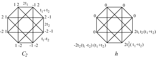
Figure 1.

In fact, the element $h$ agrees with

$$\frac{1}{2}(\tau_{1}-t_{2})(\tau_{2}-t_{2})(\tau_{1}-\tau_{2}+t_{1}+t_{2})$$

and this shows that $h$ is not a polynomial in $\tau_{1},\tau_{2},t_{1},t_{2}$ over $\mathbb{Z}$.

The problem is caused by the presence of the factor $2$ in the root system (4.1) and if we work over $\mathbb{Z}[\frac{1}{2}]$ instead of $\mathbb{Z}$, then the argument developed in the previous section works with a little modification and we obtain the following.

Theorem 4.1.

Let $\mathcal{C}_{n}$ be the labeled graph associated with the root system $\Phi(C_{n})$ of type $C_{n}$ as above. Then

$$H_{T}^{*}(\mathcal{C}_{n}){\otimes\mathbb{Z}[\frac{1}{2}]}=\mathbb{Z}{[\frac{1}{2}]}[\tau_{1},{\scriptstyle\cdots},\tau_{n},t_{1},{\scriptstyle\cdots},t_{n}]/(e_{i}({\tau}^{2})-e_{i}({t}^{2})\mid i=1,{\scriptstyle\cdots},n),$$

where $e_{i}({\tau}^{2})$ (resp. $e_{i}({t}^{2})$) is the $i^{th}$ elementary symmetric polynomial in ${\tau_{1}}^{2},{\scriptstyle\cdots},{\tau_{n}}^{2}$ (resp. ${t_{1}}^{2},{\scriptscriptstyle\cdots},{t_{n}}^{2}$).

The proof of Theorem 4.1 is almost same as that of Theorem 3.1 and we shall outline it. First we prove the following.

Lemma 4.2.

$H_{T}^{*}(\mathcal{C}_{n}){\otimes\mathbb{Z}[\frac{1}{2}]}$ is generated by $\tau_{1},{\scriptstyle\cdots},\tau_{n},t_{1},{\scriptstyle\cdots},t_{n}$ as a ring.

Proof.

The proof goes as in Lemma 3.2. When $n=1$, $\mathcal{C}_{1}$ has only one edge with vertices $1$ and $-1$, and the label of the edge is $2t_{1}$. Since $\tau_{1}(\pm 1)=\pm t_{1}$, it is easy to check that the lemma holds when $n=1$.

The key step in the proof of Lemma 3.2 was that if $h\in H_{T}^{*}(\mathcal{A}_{n})$ vanishes on $V_{i}$ for $i<q$, then one could modify $h$ so that it vanishes on $V_{i}$ for $i<q+1$ by subtracting a polynomial in $\tau_{i}$’s and $t_{i}$’s with integer coefficients from $h$, where the polynomial was of the form $G^{q}\prod_{i=1}^{q-1}(\tau_{i}-t_{n})$. In the case of type $C_{n}$, we consider

$$V_{i}^{\pm}:=\{w\in\tilde{S}_{n}\mid w(i)=\pm n\}$$

and the full labeled subgraph $\mathcal{L}_{i}^{\pm}$ of $\mathcal{C}_{n}$ with $V_{i}^{\pm}$ as the vertex set, where $\mathcal{L}_{i}^{+}$ and $\mathcal{L}_{i}^{-}$ are both isomorphic to $\mathcal{C}_{n-1}$ for each $i=1,\dots,n$.

The same argument as in the case of type $A_{n-1}$ shows that if $h\in H_{T}^{*}(\mathcal{C}_{n})$ vanishes on $V_{i}^{+}$ for $i<q$, then one can modify $h$ so that it vanishes on $V_{i}^{+}$ for $i<q+1$ by subtracting from $h$ a polynomial of the form $G_{+}^{q}\prod_{k=1}^{q-1}(\tau_{k}-t_{n})$ in $\tau_{i}$’s and $t_{i}$’s with coefficients in $\mathbb{Z}[\frac{1}{2}]$. Moreover, if $h$ vanishes on all $V_{i}^{+}$ and $V_{j}^{-}$ for $j<q$ with some $q\geq 1$, then one can modify $h$ so that it vanishes on all $V_{i}^{+}$ and $V_{j}^{-}$ for $j<q+1$ by subtracting from $h$ a polynomial in $\tau_{i}$’s and $t_{i}$’s with coefficients in $\mathbb{Z}[\frac{1}{2}]$ of the form $G_{-}^{q}\prod_{k=1}^{n}(\tau_{k}-t_{n})\prod_{l=1}^{q-1}(\tau_{l}+t_{n})$. Therefore we finally reach an element which vanishes on all $V_{i}^{\pm}$ by subtracting polynomials in $\tau_{i}$’s and $t_{i}$’s with coefficients in $\mathbb{Z}[\frac{1}{2}]$ from $h$, and this proves the lemma. ∎

It easily follows from (4.2) that $e_{i}(\tau^{2})=e_{i}(t^{2})$ for $i=1,{\scriptstyle\cdots},n$. Therefore we have a degree-preserving epimorphism

(4.3) $$\mathbb{Z}{[\frac{1}{2}]}[\tau,t]/\big{(}e_{i}(\tau^{2})-e_{i}(t^{2})\mid i=1,{\scriptstyle\dots},n\big{)}\to H_{T}^{*}(\mathcal{C}_{n}){\otimes\mathbb{Z}[\frac{1}{2}]}$$

and the same argument as in Lemma 3.4 proves the following.

Lemma 4.3.

The left hand side in (4.3) is generated by $\prod_{k=1}^{n-1}\tau_{k}^{i_{k}}$ with $i_{k}\leq 2(n-k)$ as a $\mathbb{Z}{[\frac{1}{2}]}[t]$-module.

Then, comparing the Hilbert series of the both sides in (4.3), we see that the map (4.3) is an isomorphism. The details are left to the reader.

5. Type $B_{n}$

In this section we treat type $B_{n}$. The root system $\Phi(B_{n})$ of type $B_{n}$ is given by

(5.1) $$\Phi(B_{n})=\{\pm(t_{i}+t_{j}),\ \pm(t_{i}-t_{j}),\ \pm t_{k}\mid 1\leq i<j\leq n,\ 1\leq k\leq n\}$$

and its Weyl group is the same as that of type $C_{n}$, i.e. the signed permutation group $\tilde{S}_{n}$.

Let $\mathcal{B}_{n}$ be the labeled graph associated with the root system $\Phi(B_{n})$. This labeled graph has the same vertices and edges as $\mathcal{C}_{n}$. Their labels are almost same. The only difference is that the edge $e_{w,w^{\prime}}$ with $w,w^{\prime}$ such that $w^{\prime}(i)=-w(i)$ for some $i\in[n]$ and $w^{\prime}(r)=w(r)$ for $r\ (\neq i)\in[n]$ is labeled by $t_{w(i)}$ in $\mathcal{B}_{n}$ while it is labeled by $2t_{w(i)}$ in $\mathcal{C}_{n}$.

We define $\tau_{i}$ and $t_{i}$ for $i=1,\dots,n$ by (4.2). They belong to $H_{T}^{2}(\mathcal{B}_{n})$. As remarked above, the only difference between $\mathcal{B}_{n}$ and $\mathcal{C}_{n}$ is the factor $2$ in the labels on the edges $e_{w,w^{\prime}}$ mentioned above. Therefore, if we work over $\mathbb{Z}[\frac{1}{2}]$ instead of $\mathbb{Z}$, then the same argument as in the case of type $C_{n}$ proves the following.

Lemma 5.1.

$$H_{T}^{*}(\mathcal{B}_{n})\otimes\mathbb{Z}[\frac{1}{2}]=\mathbb{Z}[\frac{1}{2}][\tau_{1},{\scriptstyle\cdots},\tau_{n},t_{1},{\scriptstyle\cdots},t_{n}]/(e_{i}({\tau}^{2})-e_{i}({t}^{2})\mid i=1,{\scriptstyle\cdots},n).$$

The above lemma is not true without tensoring with $\mathbb{Z}[\frac{1}{2}]$. We need to introduce another family of elements to generate $H_{T}^{*}(\mathcal{B}_{n})$ as a ring. Since $e_{i}(\tau)(w)\equiv e_{i}(t)(w)\pmod{2}$ for any $w$ in $\tilde{S}_{n}$, $e_{i}(\tau)-e_{i}(t)$ is divisible by $2$ and one sees that

$$f_{i}:=(e_{i}(\tau)-e_{i}(t))/2$$

is actually an element of $H_{T}^{*}(\mathcal{B}_{n})$. Note that $f_{0}=0$ since $e_{0}=1$ by definition. The purpose of this section is to prove the following.

Theorem 5.2.

Let $\mathcal{B}_{n}$ be the labeled graph associated with the root system $\Phi(B_{n})$ of type $B_{n}$ in (5.1). Then

$$H_{T}^{*}(\mathcal{B}_{n})=\mathbb{Z}[\tau_{1},{\scriptstyle\cdots},\tau_{n},t_{1},{\scriptstyle\cdots},t_{n},f_{1},{\scriptstyle\cdots},f_{n}]/I$$

where $I$ is the ideal generated by

$$\begin{split}&2f_{i}-e_{i}(\tau)+e_{i}(t)\quad(i=1,{\scriptstyle\cdots},n),\\ &\sum_{j=1}^{2k}(-1)^{j}f_{j}(f_{2k-j}+e_{2k-j}(t))\quad(k=1,{\scriptstyle\cdots},n)\end{split}$$

where $f_{\ell}=e_{\ell}(t)=0$ for $\ell>n$.

Remark.

If we set $t_{1}=\dots=t_{n}=0$, then the right hand side of the identity in Theorem 5.2 reduces to

$$\mathbb{Z}[\tau_{1},{\scriptstyle\cdots},\tau_{n},f_{1},{\scriptstyle\cdots},f_{n}]/J$$

where $J$ is the ideal generated by

$$2f_{i}-e_{i}(\tau)\quad(i=1,{\scriptstyle\cdots},n),\qquad\sum_{j=1}^{2k-1}(-1)^{j}f_{j}f_{2k-j}+f_{2k}\quad(k=1,{\scriptstyle\cdots},n)$$

where $f_{\ell}=0$ for $\ell>n$, and this agrees with the ordinary cohomology ring of the flag manifold of type $B_{n}$, see [11, Theorem 2.1].

The idea of the proof of Theorem 5.2 is same as before but the argument becomes more complicated because of the elements $f_{i}$’s. We first observe relations between $f_{i}$’s in $H_{T}^{*}(\mathcal{B}_{n})$ and those in $H_{T}^{*}(\mathcal{B}_{n-1})$.

Lemma 5.3.

For $w$ in $\tilde{S}_{n}$ with $w(q)=\pm n$, let ${w}^{\prime}$ be an element in $\tilde{S}_{n-1}$ represented by $w(1)\cdots w(q-1)w(q+1)\cdots w(n)$. We denote $f_{i}$ in $H_{T}^{*}(\mathcal{B}_{n})$ by $f_{i}^{(n)}$. Then

$$f_{i}^{(n-1)}({w}^{\prime})=\Bigg{\{}\begin{array}[]{ll}\sum_{j=0}^{i-1}f_{i-j}^{(n)}(w)(-t_{n})^{j}&\text{if $w(q)=n$,}\\ \sum_{j=0}^{i-1}f_{i-j}^{(n)}(w)t_{n}^{j}+\sum_{j=1}^{i}e_{i-j}(t_{1},{\scriptstyle\cdots},t_{n-1})t_{n}^{j}&\text{if $w(q)=-n$}.\\ \end{array}$$

Proof.

We have

$$e_{i}(t_{1},{\scriptstyle\cdots},t_{n})-e_{i}(t_{1},{\scriptstyle\cdots},t_{n-1})=e_{i-1}(t_{1},{\scriptstyle\cdots},t_{n-1})t_{n}$$

and

$$e_{i}(\tau_{1}(w),{\scriptstyle\cdots},\tau_{n}(w))-e_{i}(\tau_{1}(w^{\prime}),{\scriptstyle\cdots},\tau_{n-1}(w^{\prime}))=e_{i-1}(\tau_{1}(w^{\prime}),{\scriptstyle\cdots},\tau_{n-1}(w^{\prime}))\tau_{q}(w).$$

Therefore

$$f_{i}^{(n)}(w)-f_{i}^{(n-1)}({w}^{\prime}) = \frac{1}{2}\Big{(}e_{i}(\tau_{1}({w}),{\scriptstyle\cdots},\tau_{n}({w}))-e_{i}(t_{1},{\scriptstyle\cdots},t_{n})\Big{)}$$

$$\ \ \ -\frac{1}{2}\Big{(}e_{i}(\tau_{1}({w}^{\prime}),{\scriptstyle\cdots},\tau_{n-1}({w}^{\prime}))-e_{i}(t_{1},{\scriptstyle\cdots},t_{n-1})\Big{)}$$

$$= \frac{1}{2}\Big{(}e_{i-1}(\tau_{1}({w}^{\prime}),{\scriptstyle\cdots},\tau_{n-1}({w}^{\prime}))\tau_{q}(w)-e_{i-1}(t_{1},{\scriptstyle\cdots},t_{n-1})t_{n}\Big{)}$$

$$= \Bigg{\{}\begin{array}[]{ll}f_{i-1}^{(n-1)}(w^{\prime})t_{n}&\text{if $w(q)=n$,}\\ -\big{(}f_{i-1}^{(n-1)}(w^{\prime})+e_{i-1}(t_{1},{\scriptstyle\cdots},t_{n-1})\big{)}t_{n}&\text{if $w(q)=-n$}.\\ \end{array}$$

Using the above identity repeatedly, we obtain the following for $w$ with $w(q)=n$:

$$f_{i}^{(n-1)}({w}^{\prime}) = f_{i}^{(n)}(w)-f_{i-1}^{(n-1)}(w^{\prime})t_{n}$$

$$= f_{i}^{(n)}(w)-\big{(}f_{i-1}^{(n)}(w)-f_{i-2}^{(n-1)}(w^{\prime})t_{n}\big{)}t_{n}$$

$$= f_{i}^{(n)}(w)-f_{i-1}^{(n)}(w)t_{n}+\big{(}f_{i-2}^{(n)}(w)-f_{i-3}^{(n-1)}(w^{\prime})\big{)}t_{n}^{2}$$

$$\ \ \ \ \ \ \ \ \vdots$$

$$= \sum_{j=0}^{i-1}f_{i-j}^{(n)}(w)(-t_{n})^{j}.$$

The case $w(q)=-n$ can be treated in the same way. ∎

Lemma 5.4.

$H_{T}^{*}(\mathcal{B}_{n})$ is generated by $\tau_{1},{\scriptstyle\cdots},\tau_{n},t_{1},{\scriptstyle\cdots},t_{n},f_{1},{\scriptstyle\cdots},f_{n}$ as a ring.

Proof.

We use induction on $n$ as before. When $n=1$, $\mathcal{B}_{1}$ has only one edge with vertices $1$ and $-1$, and the label of the edge is $t_{1}$. Since $\tau_{1}(\pm 1)=\pm t_{1}$, it is easy to check that the lemma holds when $n=1$.

As before, we consider $V_{i}^{\pm}:=\{w\in\tilde{S}_{n}\mid w(i)=\pm n\}$ and the full labeled subgraph $\mathcal{L}_{i}^{\pm}$ of $\mathcal{B}_{n}$ with $V_{i}^{\pm}$ as the vertex set, where $\mathcal{L}_{i}^{+}$ and $\mathcal{L}_{i}^{-}$ are both isomorphic to $\mathcal{B}_{n-1}$ for each $i=1,\dots,n$. If $h\in H_{T}^{*}(\mathcal{B}_{n})$ vanishes on $V_{i}^{+}$ for $i<q$, then one can modify $h$ so that it vanishes on $V_{i}^{+}$ for $i<q+1$ by subtracting from $h$ an integer coefficient polynomial of the form $G_{+}^{q}\prod_{k=1}^{q-1}(\tau_{k}-t_{n})$ in $\tau_{i}$’s, $t_{i}$’s and $f_{i}$’s. In fact, we obtain $G_{+}^{q}$ as an element of $\operatorname{Map}(\tilde{S}_{n},H^{*}(BT))$ whose restriction to $\mathcal{L}_{q}^{+}$ belongs to $H_{T}^{*}(\mathcal{L}_{q}^{+})$. Since $\mathcal{L}_{q}^{+}$ is isomorphic to $\mathcal{B}_{n-1}$ and $H_{T}^{*}(\mathcal{B}_{n-1})$ is generated by $\tau_{i}$’s, $t_{i}$’s and $f_{i}$’s by the induction assumption, we can take $G_{+}^{q}$ as a polynomial in $\tau_{i}$’s, $t_{i}$’s and $f_{i}$’s with integer coefficients, where we use Lemma 5.3.

If $h$ vanishes on all $V_{i}^{+}$ and $V_{j}^{-}$ for $j<q$ with some $q\geq 1$, then one can also modify $h$ so that it vanishes on all $V_{i}^{+}$ and $V_{j}^{-}$ for $j<q+1$ by subtracting from $h$ some polynomial in $\tau_{i}$’s, $t_{i}$’s and $f_{i}$’s with integer coefficients. However, this polynomial is not of the form $G_{-}^{q}\prod_{k=1}^{n}(\tau_{k}-t_{n})\prod_{l=1}^{q-1}(\tau_{l}+t_{n})$ because $\prod_{k=1}^{n}(\tau_{k}-t_{n})(w)$ is divisible by $2$ for $w\in V_{i}^{-}$. Instead of $\prod_{k=1}^{n}(\tau_{k}-t_{n})$, we use the following element

$${\frac{1}{2}}\prod_{k=1}^{n}(\tau_{k}-t_{n}) = {\frac{1}{2}}\sum_{k=0}^{n}(-1)^{n-k}e_{k}(\tau){t_{n}}^{n-k}$$

$$= {\frac{1}{2}}\sum_{k=0}^{n}(-1)^{n-k}(2f_{k}+e_{k}(t)){t_{n}}^{n-k}$$

$$= \sum_{k=1}^{n}(-1)^{n-k}f_{k}{t_{n}}^{n-k},$$

so that the polynomial which we subtract is of the form

$$G_{-}^{q}\left(\Sigma_{k=1}^{n}(-1)^{n-k}f_{k}{t_{n}}^{n-k}\right)\prod_{l=1}^{q-1}(\tau_{l}+t_{n})$$

where $G_{-}^{q}$ is a polynomial in $\tau_{i}$’s, $t_{i}$’s and $f_{i}$’s with integer coefficients. Thus we finally reach an element which vanishes on all $V_{i}^{\pm}$ by subtracting polynomials in $\tau_{i}$’s, $t_{i}$’s and $f_{i}$’s with integer coefficients from $h$, and this proves the lemma. ∎

Lemma 5.5.

$\sum_{i=1}^{2k}(-1)^{i}f_{i}(f_{2k-i}+e_{2k-i}(t))=0$ for $k=1,{\scriptstyle\cdots},n$.

Proof.

Cleaely we have $e_{i}(\tau^{2})=e_{i}(t^{2})$ for $i=1,2,\dots,n$, namely

(5.5) $$\prod_{i=1}^{n}(1-{\tau_{i}}^{2}x^{2})=\prod_{i=1}^{n}(1-{t_{i}}^{2}x^{2}).$$

Therefore

$$0 = \prod_{i=1}^{n}(1-{\tau_{i}}^{2}x^{2})-\prod_{i=1}^{n}(1-{t_{i}}^{2}x^{2})$$

$$= \Big{(}\sum_{i=0}^{n}(-1)^{i}e_{i}(\tau)x^{i}\Big{)}\Big{(}\sum_{j=0}^{n}e_{j}(\tau)x^{j}\Big{)}-\Big{(}\sum_{i=0}^{n}(-1)^{i}e_{i}(t)x^{i}\Big{)}\Big{(}\sum_{j=0}^{n}e_{j}(t)x^{j}\Big{)}$$

$$= \Big{(}\sum_{i=0}^{n}(-1)^{i}(2f_{i}+e_{i}(t))x^{i}\Big{)}\Big{(}\sum_{j=0}^{n}(2f_{j}+e_{j}(t))x^{j}\Big{)}-\Big{(}\sum_{i=0}^{n}(-1)^{i}e_{i}(t)x^{i}\Big{)}\Big{(}\sum_{j=0}^{n}e_{j}(t)x^{j}\Big{)}$$

$$= 4\sum_{i,j=1}^{n}(-1)^{i}f_{i}f_{j}x^{i+j}+2\sum_{i,j=0}^{n}(-1)^{i}\big{(}f_{i}e_{j}(t)+f_{j}e_{i}(t)\big{)}x^{i+j}\$$

$$= 4\sum_{k=1}^{n}{\sum_{i=1}^{2k}(-1)^{i}f_{i}f_{2k-i}x^{2k}}+4\sum_{k=1}^{n}{\sum_{i=1}^{2k}(-1)^{i}f_{i}e_{2k-i}(t)x^{2k}}$$

where we used $f_{0}=0$. This implies the lemma because the coefficient of $x^{2k}$ must vanish. ∎

We abbreviate the polynomial ring $\mathbb{Z}[\tau_{1},{\scriptstyle\cdots},\tau_{n},t_{1},{\scriptstyle\cdots},t_{n},f_{1},{\scriptstyle\cdots},f_{n}]$ as $\mathbb{Z}[\tau,t,f]$. Since $2f_{i}=e_{i}(\tau)-e_{i}(t)$ by definition, it follows from Lemma 5.5 that the canonical map $\mathbb{Z}[\tau,t,f]\rightarrow H_{T}^{*}(\mathcal{B}_{n})$ induces a grade preserving map

(5.6) $$\mathbb{Z}[\tau,t,f]/I\rightarrow H_{T}^{*}(\mathcal{B}_{n}),$$

where $I$ is the ideal in Theorem 5.2, and it is an epimorphism by Lemma 5.4. Since $H_{T}^{*}(\mathcal{B}_{n})$ is a submodule of a direct sum of some $\mathbb{Z}[t]$’s, $H_{T}^{*}(\mathcal{B}_{n})$ is free over $\mathbb{Z}$. In addition, its Hilbert series is given by ${\frac{1}{(1-s^{2})^{2n}}}\prod_{i=1}^{n}(1-s^{4i})$. This can be shown by a similar computation to the proof of Lemma 3.3. In order to prove that the epimorphism (5.6) is actually an isomorphism, it suffices to verify the following Lemmas 5.6 and  5.7.

Lemma 5.6.

$\mathbb{Z}[\tau,t,f]/I$ is free over $\mathbb{Z}$.

Proof.

By Lemma 5.1 $\mathbb{Z}[\tau,t,f]/I\otimes\mathbb{Z}[\frac{1}{2}]=\mathbb{Z}[\tau,t]/I\otimes\mathbb{Z}[\frac{1}{2}]$ is isomorphic to $H_{T}^{*}(\mathcal{B}_{n})\otimes\mathbb{Z}[\frac{1}{2}]$. Since $H_{T}^{*}(\mathcal{B}_{n})$ is free over $\mathbb{Z}$, this means that $\mathbb{Z}[\tau,t,f]/I$ has no odd torsion and hence it suffices to show that $\mathbb{Z}[\tau,t,f]/I$ has no 2-torsion. If $\mathbb{Z}[\tau,t,f]/I$ has 2-torsion, then

$$F(\mathbb{Z}[\tau,t,f]/I\otimes\mathbb{Z}/2,s)>F(H_{T}^{*}(\mathcal{B}_{n})\otimes\mathbb{Z}/2,s);$$

so we will prove that

(5.7) $$F(\mathbb{Z}[\tau,t,f]/I\otimes\mathbb{Z}/2,s)\leq F(H_{T}^{*}(\mathcal{B}_{n})\otimes\mathbb{Z}/2,s).$$

Claim.

$\mathbb{Z}[\tau,t,f]/I\otimes\mathbb{Z}/2$ is generated by elements $\prod_{k=1}^{n}\tau_{k}^{i_{k}}\prod_{k=1}^{n}f_{k}^{j_{k}}$, with $i_{k}\leq n-k$ and $j_{k}\leq 1$, over $\mathbb{Z}/2[t]$.

We admit the claim for the moment and complete the proof of the lemma. If the elements $\prod_{k=1}^{n}\tau_{k}^{i_{k}}\prod_{k=1}^{n}f_{k}^{j_{k}}$ are linearly independent over $\mathbb{Z}/2[t]$, then the Hilbert series of $\mathbb{Z}[\tau,t,f]/I\otimes\mathbb{Z}/2$ (over the field $\mathbb{Z}/2$) is given by

$${\frac{1}{(1-s^{2})^{n}}}\sum_{0\leq i_{k}\leq n-k}\sum_{0\leq j_{k}\leq 1}s^{2(\sum_{k=1}^{n}i_{k}+\sum_{k=1}^{n}kj_{k})},$$

so we have

$$F(\mathbb{Z}[\tau,t,f]/I\otimes\mathbb{Z}/2,s) \leq {\frac{1}{(1-s^{2})^{n}}}\sum_{0\leq i_{k}\leq n-k}\sum_{0\leq j_{k}\leq 1}s^{2(\sum_{k=1}^{n}i_{k}+\sum_{k=1}^{n}kj_{k})}$$

$$= {\frac{1}{(1-s^{2})^{n}}}\Big{(}\sum_{0\leq i_{k}\leq n-k}\prod_{k=1}^{n}s^{2i_{k}}\Big{)}\Big{(}\sum_{0\leq j_{k}\leq 1}\prod_{k=1}^{n}s^{2kj_{k}}\Big{)}$$

$$= {\frac{1}{(1-s^{2})^{2n}}}(1-s^{2})^{n}\prod_{i=1}^{n-1}(1+\sum_{j=1}^{i}s^{2j})\prod_{i=1}^{n}(1+s^{2i})$$

$$= {\frac{1}{(1-s^{2})^{2n}}}\prod_{i=1}^{n}(1-s^{2i})\prod_{i=1}^{n}(1+s^{2i})$$

$$= {\frac{1}{(1-s^{2})^{2n}}}\prod_{i=1}^{n}(1-s^{4i})$$

$$= F(H_{T}^{*}(\mathcal{B}_{n})\otimes\mathbb{Z}/2,s).$$

This proves the desired inequality (5.7).

In the sequel it remains to show the claim above and for that it suffices to verify the following (I) and (II):

(I) Elements $\prod_{k=1}^{n}\tau_{k}^{i_{k}}\prod_{k=1}^{n}f_{k}^{j_{k}}$, with $i_{k}\leq n-k$, generate $\mathbb{Z}[\tau,t,f]/I$ as a $\mathbb{Z}[t]$-module, in particular, they generate $\mathbb{Z}/2[\tau,t,f]/I$ as a $\mathbb{Z}/2[t]$-module.
(II) Elements $f_{1}^{{j_{1}}^{\prime}}\cdots f_{n}^{{j_{n}}^{\prime}}$ can be written as a linear combination of $f_{1}^{{j_{1}}}\cdots f_{n}^{{j_{n}}}$ with $j_{k}\leq 1$ over $\mathbb{Z}/2[t]$.

Proof of (I). Clearly the elements $\prod_{k=1}^{n}\tau_{k}^{i_{k}}\prod_{k=1}^{n}f_{k}^{j_{k}}$, with no restriction on exponents, generate $\mathbb{Z}[\tau,t,f]/I$ as a $\mathbb{Z}[t]$-module. We have an identity

$$\prod_{i=1}^{p}{\frac{1}{1-\tau_{i}x}} = \prod_{i=p+1}^{n}(1-\tau_{i}x)\prod_{i=1}^{n}(1+\tau_{i}x)\prod_{i=1}^{n}{\frac{1}{1-{t_{i}}^{2}x^{2}}}$$

$$= \Big{(}\sum_{i=0}^{n-p}(-1)^{i}e_{i}(\tau_{p+1},{\scriptstyle\cdots},\tau_{n})x^{i}\Big{)}\Big{(}\sum_{j=0}^{n}e_{j}(\tau_{1},{\scriptstyle\cdots},\tau_{n})x^{j}\Big{)}\sum_{k=0}^{\infty}h_{k}(t^{2})x^{2k}$$

$$= \Big{(}\sum_{i=0}^{n-p}(-1)^{i}e_{i}(\tau_{p+1},{\scriptstyle\cdots},\tau_{n})x^{i}\Big{)}\Big{(}\sum_{j=0}^{n}(2f_{j}+e_{j}(t))x^{j}\Big{)}\sum_{k=0}^{\infty}h_{k}(t^{2})x^{2k}$$

where the first equality in (5) follows from (5.5).

Comparing coefficients of $x^{n+1-p}$ in (5), we have

(5.10) $$h_{n+1-p}(\tau_{1},{\scriptstyle\cdots},\tau_{p})=\sum_{i+j+2k=n+1-p,\ j+k>0}(-1)^{i}e_{i}(\tau_{p+1},{\scriptstyle\cdots},\tau_{n})(2f_{j}+e_{j}(t))h_{k}(t^{2}).$$

On the other hand, we have

$$\sum_{j=0}^{i}e_{j}(\tau_{1},{\scriptstyle\cdots},\tau_{p})e_{i-j}(\tau_{p+1},{\scriptstyle\cdots},\tau_{n})=e_{i}(\tau)=2f_{i}+e_{i}(t)\text{$\ \ \ \ $for any $i$},$$

that is,

(5.11) $$e_{i}(\tau_{p+1},{\scriptstyle\cdots},\tau_{n})=2f_{i}+e_{i}(t)-\sum_{j=1}^{i}e_{j}(\tau_{1},{\scriptstyle\cdots},\tau_{p})e_{i-j}(\tau_{p+1},{\scriptstyle\cdots},\tau_{n})\text{$\ \ \ \ $for any $i$}.$$

Then the same argument as in the latter part of the proof of Lemma 3.4 using (5.11) shows that $e_{i}(\tau_{p+1},{\scriptstyle\cdots},\tau_{n})$ can be written as a linear combination of $\prod_{k=1}^{p}\tau_{k}^{i_{k}}\prod_{k=1}^{n}f_{k}^{j_{k}}$, with $i_{k}\leq i$, over $\mathbb{Z}[t]$. This fact and (5.10) together with (3.16) show that $\tau_{p}^{n+1-p}$ is a polynomial in $\tau_{1},{\scriptstyle\cdots},\tau_{p}$, $t_{i}$’s and $f_{i}$’s with the exponent of $\tau_{p}$ less than or equal to $n-p$. Therefore the elements $\prod_{k=1}^{n}\tau_{k}^{i_{k}}\prod_{k=1}^{n}f_{k}^{j_{k}}$ with $i_{k}\leq n-k$, generate $\mathbb{Z}[\tau,t,f]/I$ as a $\mathbb{Z}[t]$-module.

Proof of (II). It follows from Lemma 5.5 that

$$f_{k}^{2}=(-1)^{k+1}\Big{(}2\sum_{i=1}^{k-1}(-1)^{i}f_{i}f_{2k-i}+\sum_{i=1}^{2k}(-1)^{i}f_{i}e_{2k-i}(t)\Big{)}\quad\text{for $k=1,\dots,n$.}$$

In $\mathbb{Z}[\tau,t,f]/I\otimes\mathbb{Z}/2$, we can disregard $2\sum_{i=1}^{k-1}f_{i}f_{2k-1}$; so ${f_{k}}^{2}$ can be written as a linear combination of $f_{i}$’s over $\mathbb{Z}/2[t]$. This proves (II) and completes the proof of the claim. ∎

Lemma 5.7.

$\displaystyle{F(\mathbb{Z}[\tau,t,f]/I,s)={\frac{1}{(1-s^{2})^{2n}}}\prod_{i=1}^{n}(1-s^{4i})}$.

Proof.

The epimorphism (5.6) means

(5.12) $$F(H_{T}^{*}(\mathcal{B}_{n}),s)\leq F(\mathbb{Z}[\tau,t,f]/I,s).$$

In addition, since $\mathbb{Z}[\tau,t,f]/I$ and $H_{T}^{*}(\mathcal{B}_{n})$ are free over $\mathbb{Z}$,

(5.13) $$F(H_{T}^{*}(\mathcal{B}_{n})\otimes\mathbb{Z}/2,s)=F(H_{T}^{*}(\mathcal{B}_{n}),s)$$

and

(5.14) $$F(\mathbb{Z}[\tau,t,f]/I\otimes\mathbb{Z}/2,s)=F(\mathbb{Z}[\tau,t,f]/I,s).$$

It follows from (5), (5.12), (5.13) and (5.14) that

$$F(\mathbb{Z}[\tau,t,f]/I,s)=F(H_{T}^{*}(\mathcal{B}_{n}),s)={\frac{1}{(1-s^{2})^{2n}}}\prod_{i=1}^{n}(1-s^{4i}),$$

proving the lemma. ∎

Thus the proof of Theorem 5.2 has been completed.

6. Type $D_{n}$

In this section we will treat type $D_{n}$. The root system $\Phi(D_{n})$ of type $D_{n}$ is given by

$$\Phi(D_{n})=\{\pm(t_{i}+t_{j}),\ \pm(t_{i}-t_{j})\mid 1\leq i<j\leq n\}$$

and its Weyl group is the index two subgroup $\tilde{S}^{+}_{n}$ of $\tilde{S}_{n}$ defined by

$$\tilde{S}^{+}_{n}:=\{w\in\tilde{S}_{n}\mid\text{the number of $i\in[n]$ with $w(i)<0$ is even}\}.$$

Theorem 6.1.

Let $\mathcal{D}_{n}$ be the labeled graph associated with the root system $\Phi(D_{n})$ of type $D_{n}$ above. Then

(6.1) $$H_{T}^{*}(\mathcal{D}_{n})=\mathbb{Z}[\tau_{1},{\scriptstyle\cdots},\tau_{n},t_{1},{\scriptstyle\cdots},t_{n},f_{1},{\scriptstyle\cdots},f_{n-1}]/I,$$

where $I$ is the ideal generated by

$$\begin{split}&2f_{i}-e_{i}(\tau)+e_{i}(t)\quad(i=1,{\scriptstyle\cdots},n-1),\\ &\sum_{j=1}^{2k}(-1)^{j}f_{j}(f_{2k-j}+e_{2k-j}(t))\quad(k=1,{\scriptstyle\cdots},n),\\ &e_{n}(\tau)-e_{n}(t),\end{split}$$

where $f_{\ell}=0$ for $\ell\geq n$ and $e_{\ell}(t)=0$ for $\ell>n$.

Remark.

(1) Similarly to $\mathcal{D}_{n}$, one can define a labeled graph $\mathcal{D}_{n}^{-}$ with $\tilde{S}_{n}\backslash\tilde{S}_{n}^{+}$ as the vertex set on which $\tilde{S}_{n}^{+}$ acts. One sees that $H_{T}^{*}(\mathcal{D}_{n}^{-})$ agrees with the right hand side of (6.1) with $e_{n}(\tau)-e_{n}(t)$ replaced by $e_{n}(\tau)+e_{n}(t)$.

(2) If we set $t_{1}=\dots=t_{n}=0$, then the right hand side of the identity in Theorem 6.1 reduces to

$$\mathbb{Z}[\tau_{1},{\scriptstyle\cdots},\tau_{n},f_{1},{\scriptstyle\cdots},f_{n-1}]/J$$

where $J$ is the ideal generated by

$$2f_{i}-e_{i}(\tau)\ \ (i=1,{\scriptstyle\cdots},n-1),\quad\sum_{j=1}^{2k-1}(-1)^{j}f_{j}f_{2k-j}+f_{2k}\ \ (k=1,{\scriptstyle\cdots},n),\quad e_{n}(\tau)$$

where $f_{\ell}=0$ for $\ell\geq n$, and this agrees with the ordinary cohomology ring of the flag manifold of type $D_{n}$, see [11, Corollary 2.2].

Outline of proof.

The proof is almost same as the case of type $B_{n}$ but needs some modification. We shall list them.

(1) $e_{n}(\tau)=e_{n}(t)$ in the type $D_{n}$ case since the number of $i\in[n]$ with $w(i)<0$ is even for $w\in\tilde{S}^{+}_{n}$. So $f_{n}=(e_{n}(\tau)-e_{n}(t))/2=0$ in the case of type $D_{n}$.

(2) Let $V_{i}^{\pm}$ and $\mathcal{L}_{i}^{\pm}$ be defined similarly to the case of type $B_{n}$. Then $\mathcal{L}_{i}^{+}$ is naturally isomorphic to $\mathcal{D}_{n-1}$ but $\mathcal{L}_{i}^{-}$ is not because the number of $j\in[n]\backslash\{i\}$ with $w(j)<0$ is odd for $w\in\tilde{S}_{n}^{+}$. Therefore the induction argument as in Lemma 3.2 does not work. To overcome this, we need to apply the induction argument to $\mathcal{D}_{n}$ and $\mathcal{D}_{n}^{-}$ simultaneously because $\mathcal{L}_{i}^{-}$ is isomorphic to $\mathcal{D}_{n-1}^{-}$. Note that if we start with $\mathcal{D}_{n}^{-}$, then $\mathcal{L}_{i}^{+}$ (for $\mathcal{D}_{n}^{-}$) is isomorphic to $\mathcal{D}_{n-1}^{-}$ while $\mathcal{L}_{i}^{-}$ (for $\mathcal{D}_{n}^{-}$) is isomorphic to $\mathcal{D}_{n-1}$.

(3) If $h\in H_{T}^{*}(\mathcal{D}_{n})$ vanishes on $V_{i}^{+}$ for $i<q$, then one can modify $h$ so that it vanishes on $V_{i}^{+}$ for $i<q+1$ by subtracting from $h$ a polynomial of the form $G_{+}^{q}\prod_{k=1}^{q-1}(\tau_{k}-t_{n})$ in $\tau_{i}$’s and $t_{i}$’s with integer coefficients. Therefore, we may assume that $h$ vanishes on all $V_{i}^{+}$. Then $h(w)$ for $w\in V_{1}^{-}$ is divisible by $\prod_{k=2}^{n}(t_{w(k)}-t_{n})=\prod_{k=2}^{n}(\tau_{k}-t_{n})(w)$. (Note that $w$ is connected to a vertex in $V_{i}^{+}$ by an edge for $i>1$, but not to any vertex in $V_{1}^{+}$. This is the reason why $i=1$ is missing in the product above.) However, since $f_{n}=0$ (i.e. $e_{n}(\tau)=e_{n}(t)$) as mentioned in (1) above in the case of type $D_{n}$, it follows from (5) that

(6.2) $$P:=-\frac{1}{2t_{n}}\prod_{k=1}^{n}(\tau_{k}-t_{n})=\sum_{k=1}^{n-1}(-1)^{n-1-k}f_{i}t_{n}^{n-1-k}.$$

$P$ is a polynomial in $t_{i}$’s and $f_{i}$’s with integer coefficients, vanishes on all $V_{i}^{+}$ and takes the value $\prod_{k=2}^{n}(t_{w(k)}-t_{n})$ on $w\in V_{1}^{-}$. Therefore, using the polynomial $P$ in (6.2), one can modify $h$ so that it vanishes on all $V_{i}^{+}$ and $V_{1}^{-}$ by subtracting a polynomial in $\tau_{i}$’s and $t_{i}$’s with integer coefficients. If $h$ vanishes on all $V_{i}^{+}$ and $V_{j}^{-}$ for $j<q$ with some $q\geq 2$, then one can modify $h$ so that it vanishes on all $V_{i}^{+}$ and $V_{j}^{-}$ for $j<q+1$ by subtracting from $h$ an integer coefficient polynomial of the form $G_{-}^{q}P\prod_{l=1}^{q-1}(\tau_{l}+t_{n})$. Therefore we finally reach an element which vanishes on all vertices of $\mathcal{D}_{n}$. This shows that $H_{T}^{*}(\mathcal{D}_{n})$ is generated by $\tau_{i}$’s, $t_{i}$’s and $f_{i}$’s as a ring. The same argument shows that $H_{T}^{*}(\mathcal{D}_{n}^{-})$ is also generated by $\tau_{i}$’s, $t_{i}$’s and $f_{i}$’s as a ring.

(4) A similar argument to the case of type $B_{n}$ shows that the right hand side in (6.1) is torsion free over $\mathbb{Z}$ and the Hilbert series of the both sides in (6.1) coincide, in fact, they are given by ${\frac{1-s^{2n}}{(1-s^{2})^{2n}}}\prod_{i=1}^{n-1}(1-s^{4i})$. The same is true for $H_{T}^{*}(\mathcal{D}_{n}^{-})$. ∎

Acknowledgment. The authors would like to thank Takeshi Ikeda, Shizuo Kaji, Leonardo C. Mihalcea, Hiroshi Naruse and Takashi Sato for information on the integral cohomology rings of flag manifolds and for pointing out mistakes in an earlier version.

References

- [1] Y. Fukukawa, The cohomology ring of the GKM graph of a flag manifold, Trends in Mathematics - New Series, Information Center for Mathematical Sciences, vol. 12, No. 1, 2010 (Toric Topology Workshop KAIST 2010), 121–123.
- [2] Y. Fukukawa. The cohomology ring of the GKM graph of a flag manifold of type , arXiv:1207.5229.
- [3] W. Fulton, Young Tableaux, London Math. Soc. Student Texts 35, 1997.
- [4] W. Fulton and P. Pragacz, Schubert Varieties and Degeneracy Loci, Lect. Notes in Math. 1689, Springer, 1998.
- [5] M. Goresky, R. Kottwitz and R. MacPherson, Equivariant cohomology, Koszul duality and the localisation theorem, Invent. Math. 131 (1998) 25–83.
- [6] V. Guillemin and S. Sternberg, Supersymmetry and Equivariant de Rham Theory, Springer, Berlin–Heidelberg–New York, 1999.
- [7] V. Guillemin and C. Zara, 1-skeleta, Betti numbers and equivariant cohomology, Duke Math. J. 107 (2001) 283–349.
- [8] V. Guillemin, T. Holm and C. Zara, A GKM description of the equivariant cohomology ring of a homogeneous space, J. Algebraic Combin. 23 (2006), 21–41.
- [9] M. Harada, A. Henriques and T. Holm, Computation of generalized equivariant cohomologies of Kac-Moody flag varieties, Adv. Math. 197 (2005), 198–221.
- [10] H. Maeda, M. Masuda and T. Panov, Torus graphs and simplicial posets, Adv. Math. 212 (2007), 458–483.
- [11] H. Toda and T. Watanabe, The integral cohomology ring of and , J. Math. Kyoto Univ. 14-2 (1974), 257–286.