Zipf’s law unzipped

Abstract

Why does Zipf’s law give a good description of data from seemingly completely unrelated phenomena? Here it is argued that the reason is that they can all be described as outcomes of a ubiquitous random group division: the elements can be citizens of a country and the groups family names, or the elements can be all the words making up a novel and the groups the unique words, or the elements could be inhabitants and the groups the cities in a country, and so on. A Random Group Formation (RGF) is presented from which a Bayesian estimate is obtained based on minimal information: it provides the best prediction for the number of groups with $k$ elements, given the total number of elements, groups, and the number of elements in the largest group. For each specification of these three values, the RGF predicts a unique group distribution $N(k)\propto\exp(-bk)/k^{\gamma}$, where the power-law index $\gamma$ is a unique function of the same three values. The universality of the result is made possible by the fact that no system specific assumptions are made about the mechanism responsible for the group division. The direct relation between $\gamma$ and the total number of elements, groups, and the number of elements in the largest group, is calculated. The predictive power of the RGF model is demonstrated by direct comparison with data from a variety of systems. It is shown that $\gamma$ usually takes values in the interval $1\leq\gamma\leq 2$ and that the value for a given phenomena depends in a systematic way on the total size of the data set. The results are put in the context of earlier discussions on Zipf’s and Gibrat’s laws, $N(k)\propto k^{-2}$ and the connection between growth models and RGF is elucidated.

1 Introduction

The remarkable feature that power-law distributions are commonly encountered in a huge variety of seemingly very different systems has a long history: the first discovery seems to go back to Pareto’s paper from 1896 concerning the uneven distribution of incomes [1]. Some twenty years later Auerbach in Ref. [2] found the same power-law distributions for city sizes. Subsequently, George Kingsley Zipf found power-law distributions for the word frequency in written texts and this empirical finding became known as Zipf’s law [3, 4, 5], although the first discovery for the case of word frequencies was made some twenty years earlier by J. K. Estroup [6]. By now the literature related to Zipf’s law is immense and spans basically all fields: economy, sociology, linguistics, physics, mathematical statistics, to mention a few. A short history can be found in Ref. [7].

A large amount of the literature on Zipf’s law is concerned with empirically finding systems which obey Zipf’s law [8], the precise mathematical form of the distribution which should be associated with Zipf’s empirical law [9], statistical methods for establishing whether or not one mathematical form fits the empirical data better than another, and last but not least various methods for data analysis in order to find the precise value of the power-law exponent for the alleged power law. This is not a concern of the present paper. Instead we focus on the question “Why?”: Why does Zipf’s law give a good description of data from seemingly completely unrelated phenomena?

The present work stems from a specific remark made by Herbert Simon in Ref. [10] ‘No one supposes that there is any connection between horse-kicks suffered by soldiers in the German army and blood cells on a microscopic slide other than that the same urn scheme provides a satisfactory abstract model for both phenomena.’ This is precisely the view taken in the present paper: if a vast amount of seemingly unrelated phenomena share a common characteristic, this characteristic cannot depend on the details of the system but must be traced to a global feature. Simon’s explicit attempt to find such an abstract model, the Simon growth model, was criticized by Benoit Mandelbrot in Ref. [11], who instead argued that a growth model was not adequate and that the common feature should be associated with information and entropy [12]. These opposite view-points led to a heated argument between Simon and Mandelbrot [7]. From our perspective, both were right: The common element must be a global abstract model and information is the shared quantity which decides the characteristics.

The basic element proposed here is that the abstract common feature is the division into groups. The generic model for this is numbered balls divided into boxes. As examples, we take people (balls) divided into cities (boxes), people (balls) divided into family names (boxes), and words from a novel (balls) divided into number of occurrences in the text (boxes). We then use information theory to obtain the best (Bayesian) prediction of the box-size distribution based on maximum mutual information.

In section 2, we present the empirical data to which we compare our predictions. In the following section 3, we describe and explain the Random Group Formation (RGF) model. In section 4, the empirical data is directly compared with the explicit predictions of the RGF model. The reason for a systematic size change of the power-law exponent is explained and exemplified by data from novels. In section 5, the connection between the equilibrium maximum-entropy distribution and Gibrat’s growth model [13, 14] is discussed and it is explained that the power-law distribution $P(k)\propto k^{-2}$ is indeed an equilibrium feature rather than a growth feature. Finally, section 6 contains a summary and concluding remarks. In addition, various more detailed clarifications are relegated to three appendices.

2 What do we want to explain?

Table 1: Basic quantities of the datasets. $M$ is the total number of elements, $N$ is the number of groups, $k_{\max}$ is the size of the largest group, and $k_{0}$ is the size of the smallest group shown in the dataset.

• 	$M$	$N$	$k_{\max}$	$k_{0}$
  US counties	277 537 173	2 445	9 519 338	$10^{4}$
  French communes	51 107 816	9 011	852 395	$10^{3}$
  US family names	242 121 073	151 671	2 376 206	$10^{2}$
  Korean family names	45 974 571	244	9 925 949	$10^{2}$
  Hardy	1 342 258	30 744	74 165	$10^{0}$
  Melville	743 666	30 122	49 136	$10^{0}$

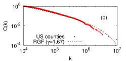
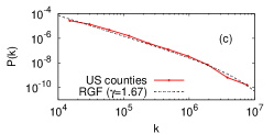
Figure 1: Population distribution for the counties in US from the year 2000 survey (source: US Census 2000 [15]). (a) Raw-data in a log-log plot; (b) Cumulative C(k); (c) Binned P(k). Dashed curves in (b) and (c) give the RGF prediction for the dataset.

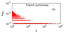
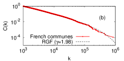
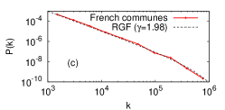
Figure 2: Distribution of population of French communes (source: City Population [16]). (a) Raw-data in a log-log plot; (b) Cumulative C(k); (c) Binned P(k). Dashed curves in (b) and (c) give the RGF prediction for the dataset.

The question we want to address is best illustrated by explicit examples. Three seemingly completely unrelated phenomena are chosen: the city-size distribution of a country, family-name frequencies for a country, and the word-frequency distribution in novels. Two examples are given in each case. Figure 1 shows the county-size distribution in United States (US) for year 2000 [15] and in this case the total population is $M=2.8\times 10^{8}$, the number of counties $N=2445$ and the largest county is Los Angeles with $k_{\max}=9.5\times 10^{6}$ inhabitants (see table 1). Figure 1(a) gives the average number of counties having $k$ inhabitants and since only rarely two counties have precisely the same number, basically all data points fall on the line $1/N$. However, smaller counties are much more common than very large and in figure 1(b) this feature is clearly displayed by instead plotting the number of counties which have population larger than $k$. This is usually called the cumulative distribution, denoted by $C(k)$, and normalized such that $C(k_{0})=1$, where $k_{0}$ is the size of the smallest county in the dataset. The interesting thing to note is the broadness of the distribution: this type of distribution is often called “fat-tailed”. Figure 1(c) illustrates the same feature by log-binning the raw data. The resulting distribution $P(k)$ is also “fat-tailed” and, since $C(k)$ is related to $P(k)$ by $\sum_{k}P(k)$, figure 1(b) and figure 1(c) basically carry the same information. $P(k)$ is called the frequency distribution and is normalized such that $\sum_{k_{0}}P(k)=1$.

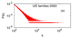
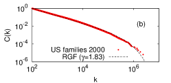
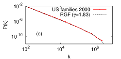
Figure 3: Distribution of US family names (source: US Census 2000 [17]). (a) Raw-data in a log-log plot; (b) Cumulative C(k); (c) Binned P(k). Dashed curves in (b) and (c) give the RGF prediction for the dataset.

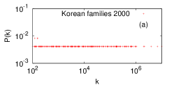
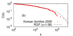
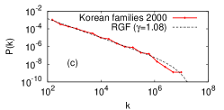
Figure 4: Distribution of Korean family names (source: 2000 South Korea Census [18]). (a) Raw-data in a log-log plot; (b) Cumulative C(k); (c) Binned P(k). Dashed curves in (b) and (c) give the RGF prediction for the dataset.

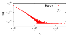
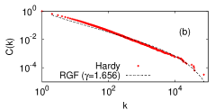
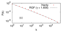
Figure 5: Distribution of word-frequencies for the author Thomas Hardy (source: see Table I of Ref. [19]) (a) Raw-data in a log-log plot; (b) Cumulative C(k); (c) Binned P(k). Dashed curves in (b) and (c) give the RGF prediction for the dataset.

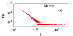
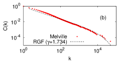
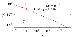
Figure 6: Distribution of word-frequencies for the author Herman Melville (source: see Table I of Ref. [19]) (a) Raw-data in a log-log plot; (b) Cumulative C(k); (c) Binned P(k). Dashed curves in (b) and (c) give the RGF prediction for the dataset.

The first thing one may ask is if this fat-tailed feature is specific to county sizes in US. The answer that it indeed is a typical feature of city distributions was first noted by Auerbach in 1913 [2] and has since then been amply verified. We illustrate this in figure 2 by including the communal sizes of France [16]. In this case the total population is $M=5.1\times 10^{7}$, the number of communes $N=9011$ and the largest commune is Marseille with $k_{\max}=8.5\times 10^{5}$ inhabitants (see table 1). The data is displayed in the same way and the similarity of the shape of the fat-tailed distribution is striking. What is the reason for this similarity? The first thought might be that it must be connected to some specific human endeavor of creating towns for reasons related to fertility, immigration, economics, commerce and defense and hindered by factors like epidemics, emigration, war, famine and earthquakes. However, this thought is to some extent superseded by figure 3, which shows that the family names in US are distributed in a very similar way (data from US Census 2000 [17]). In this case the total number of persons in the dataset is $M=2.4\times 10^{8}$, the number of family names is $N=1.5\times 10^{5}$, and the most common name Smith has $k_{\max}=2.4\times 10^{6}$ carriers. Thus “fat tails” are not exclusive for city-size distributions. The second example of family names is from Korea (data taken from 2000 South Korea Census [18]). As apparent from figure 4, this distribution also has a “fat tail”. However, the fall-off in the log-log plot is slower than for the US family names. Nevertheless, a common feature is the fat tails. Perhaps one could argue that the common factor between city sizes and family names is that in both cases the basic entity are people and so that the reason could be linked to some human sociology [20, 21]. However, figure 5 and figure 6 show that the same fat-tailed feature remains true for the word-frequency distribution of words of an author. Figure 5 shows the data compiled from a large set of Thomas Hardy’s novels (the data set is taken from Table I of Ref. [19] and is obtained by adding together novels by Hardy into a single giant novel). In this case, the total number of words is $M=1.3\times 10^{6}$, the number of distinct words is $N=3.0\times 10^{4}$ and the most common word is ‘the’ which appears $k_{\max}=7.4\times 10^{4}$ times. Again the same type of “fat tailed” distribution, as for the previous cases, is obtained. The second example of word-frequency of an authors is Herman Melville (the data is obtained in the same way as for Hardy and is taken from Table I of Ref. [19]). This time $M=7.4\times 10^{5}$, $N=3.0\times 10^{4}$ and the number of ‘the’ is $k_{\max}=4.9\times 10^{4}$. The result is very much the same as for the other cases.

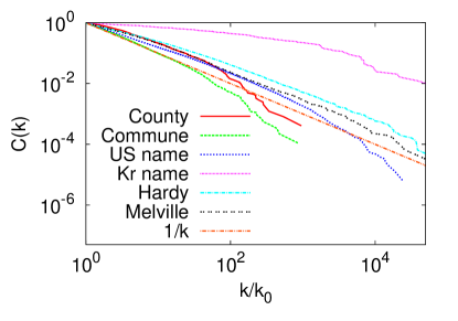
Figure 7: Direct comparison of the raw data for the six cases in the cumulative representation $C(k)$. The horizontal axis is plotted as $k/k_{0}$ where $k_{0}$ is the size of the smallest group in respective dataset. Although the functional forms are clearly different in detail for all the cases, the “fat tails” are a shared feature.

Figure 7 gives a direct comparison between the raw data for the six cases by using the cumulative representation $C(k/k_{0})$ where $k_{0}$ is the size of the smallest group of the dataset in each case. The distributions in all cases are ”fat tailed”. However the precise functional form differs in every case. Of the pairs for the three different phenomena, the word frequencies for Hardy and Melville come closest to be similar. Nevertheless, they are clearly different. The two city-size distributions are also rather similar but not as close as the two word-frequency distributions. Finally the two family-name distributions are quite different. On the other hand, the US family names and the Melville’s word frequency have a substantial overlap for smaller $k/k_{0}$. The full drawn straight line in figure 7 is the prediction of Zipf’s law $C(k)\propto 1/k$ [3]. As seen from the figure, Zipf’s law does not give a particular good mathematical description of the data. All the data sets fall on convex curves in a log-log plot and only the French commune data follow Zipf’s law over a limited interval for smaller $k$. You can argue that all the data sets to some extent follow a power-law $k^{-\alpha}$ with different power-law indices $\alpha\leq 1$ in limited regions for smaller $k$. In such a case it is only the Zipf value $\alpha=1$ which is too restricted, so that the more general power-law form could still be a significant feature. However, the undeniable fact is that all the curves are somewhat convex and hence that the power-law form does not give a complete mathematical representation of the data. Nevertheless, one can argue that Zipf’s law catches the essential fact that the distributions are broad and have fat tails and that the broadness to a first approximation can be estimated by power-law distributions, albeit with different power-law indices. However, from such a view point, it is really the broadness which is the essential thing: the power-law approximations per se may not have any direct bearing on the understanding.

There are two possible hypotheses you can start from: either one argues that the “fat-tailed” distributions are essentially system-specific and that the similarity of the distributions is just accidental and hence of no particular significance, or you can side with Herbert Simon in Ref. [10] and argue that the similarities imply an underlying system-independent stochastic process which accounts for the “fat tails”. In this paper, we pursue the latter possibility.

3 Random Group Formation

A common feature of all the data-sets in section 2 is that they on an abstract level can be described as objects divided into categories. The point made here is that, considering the immense variety of systems which display the same type of “fat tails”, it seems hard to imagine any other general shared feature. The question addressed here is what can be deduced about the size of the categories solely based on this common feature.

The starting point for the RGF model is as follows: You have $M$ numbered balls and $N$ boxes. The box sizes are $N(k)$, which means that a box of size $k$ has $k$ distinct slots which a ball can occupy. There are hence in total $M$ distinct slots and since you have no other knowledge, you assume that the probability of finding a specific ball at any address is equal. This is the Bayesian assumption. This means that the chance of finding a specific ball at a specific address is $P_{\rm dice}=1/M$. To make it less abstract, one can consider people divided into towns. A town of size $k$ has $k$ addresses where a person can live. You can imagine that the persons move around so as to come close to friends and suitable job opportunities. However, the motivation and initiative differ quite a lot. But if you do not have any information of these system-specific driving forces, your best guess is that any person has an equal probability to live at any address.

Under this Bayesian assumption of equal address probability, what is the best estimate you can make for the distribution $N(k)$? One may then note that $P(k)=N(k)/N$ can be viewed as a probability distribution. This means that, if you know $P(k)$, then a typical expected $N(k)$ is obtained by randomly drawing $N$ box-sizes from the probability distribution $P(k)$. The most likely $P(k)$ corresponds to the maximum entropy of $S[P(k)]=-\sum_{k}P(k)\ln P(k)$ under the constraints that $M$ and $N$ are given, together with the constraint given by the condition $P_{\rm dice}=1/M$. The last constraint can be handled by maximum mutual information [22] or equivalently by minimum information cost, as explained in A. The information cost enters as follows: the information to localize a ball with no additional knowledge is $I_{\rm total}=\ln M$ (in nats). The information needed to localize a ball, if you know that it is contained in a box of size $k$, is $\ln[kN(k)]$. This means that if you draw a value $k$ from the probability function $P(k)$, then $\ln[kN(k)]$ is the information it will cost you to localize a specific ball belonging to this $k$ value: the information cost is defined as the additional info which on the average is needed to localize a ball if you know the box size, $I_{\rm cost}=\sum_{k}P(k)\ln[kN(k)]$. The best estimate of $P(k)$ is obtained by minimizing the information cost subject to the $M$ and $N$ constraints, i.e., minimizing $G([P(k)]$

$$G([P(k)])=I_{\rm cost}[P(k)]+c_{1}\sum_{k}P(k)+c_{2}\sum_{k}kP(k)$$ (1)

where $c_{1}$ and $c_{2}$ are positive constants. It is interesting to note that $G([P(k)])$ can be regarded as the total information cost: each additional constraint means that information is added to the specification of the system and hence adds to the cost. The variational solution is

$$P(k)=A\frac{\exp(-bk)}{k}$$ (2)

where $A$ and $b$ are determined by the conditions $\sum_{k=1}^{M}P(k)=1$ and $\sum_{k=1}^{M}kP(k)=\left<k\right>=M/N$. This distribution is hence the most likely distribution provided that you randomly place $M$ numbered balls into $N$ boxes under the condition that the chance of finding a specific ball in a specific slot is equal. A crucial observation is that equal chance means no preference and that any preference means additional knowledge. Additional knowledge means larger a priori knowledge which means smaller entropy for the distribution $P(k)$. Thus any additional a priori knowledge means smaller entropy. This observation makes it possible to go one step further without losing generality.

In case of the real systems described in the preceding section, one can think of innumerable processes involved in creating the data. Among these there are likely to be processes which breaks the no preference condition and hence lower the entropy of the distribution $P(k)$. If we a priori assume that the entropy is lowered by the amount $\Delta S$, caused by the combined effect of all such unknown non-preference breaking processes, then this can simply be incorporated into the variational estimate as yet another Lagrangian constraint

$$G([P(k)])=I_{cost}([P(k)])+c_{1}\sum_{k}P(k)+c_{2}\sum_{k}kP(k)+c_{3}S[P(k)]$$ (3)

where $c_{3}$ is an additional Lagrangian multiplier and the solution is

$$P(k)=A\frac{exp(-bk)}{k^{\gamma}}$$ (4)

where $\gamma=\frac{1}{1-c_{3}}$ and the multipliers are determined by the three conditions $\sum_{k=1}^{M}P(k)=1$, $\sum_{k=1}^{M}kP(k)=\left<k\right>$ and $-\sum_{k=1}^{M}P(k)\ln P(k)=\Delta S$.

To turn this into a predictive estimate, one also needs an estimate of $\Delta S$. Here the particular functional form of $P(k)$ given by (4) provides a convenient estimate of $\Delta S$; since $\Delta S$ lowers the entropy of $P(k)$, it always makes the “fat tail” less broad. This means that it also lowers the value $k_{\max}$. The value of the member of the largest group is well defined for each dataset and can hence be used as an input parameter. The connection between $k_{\max}$ and $P(k)$ given by (4) can be obtained as follows: determine the value $k_{c}$ for which $C(k_{c})=1/N$ which means that there is on the average precisely one box in the interval $[k_{c},M]$. The average size of this box is given by $\sum_{k_{c}}^{M}kP(k)=\left<k_{\max}\right>$; $\left<k_{max}\right>$ is the best possible estimate of $k_{\max}$ for a dataset generated by the probability distribution $P(k)$. This means that given $M$, $N$, and $k_{\max}$, the RGF model provides you with a unique prediction for $P(k)$, where $P(k)$ is obtained from a set of self-consistent equations. More details on the RGF model are given in B.

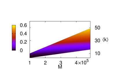
Figure 8: The parameters determining the RGF function $\propto\exp(-bk)/k^{\gamma}$ for a fixed $\gamma=1.8$: $M$ is given on the horizontal axis and $\left<k\right>$ on the horizontal right axis, while $\left<k_{\max}\right>/M$ is color coded. The figure illustrates that if you know any three of the four parameters $M$, $N$, $\left<k_{\max}\right>$ and $\gamma$, the fourth is uniquely determined by the RGF function.

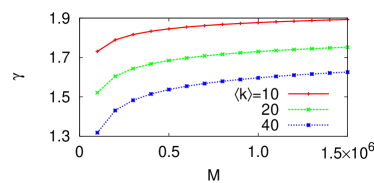
Figure 9: Dependence of $\gamma$ on the total number of elements $M$ for fixed $\left<k\right>=M/N$.

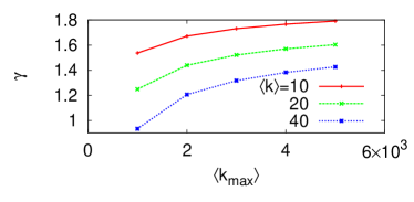
Figure 10: Dependence of $\gamma$ on the number of elements in the largest group, $\left<k_{\max}\right>$, for fixed $\left<k\right>=M/N$.

Figure 8 shows the possible solution for a specific value of $\gamma$ as a function of $M$, $\left<k\right>=M/N$, and $k_{\max}$ (where $k_{\max}$ is color coded). One notes that for any given $M$ and $\left<k\right>$, there is a whole range of possible $k_{\max}$ values and this range depends explicitly on the system size $M$. Figure 9 illustrates how $\gamma$ depends on $M$ for fixed $\left<k\right>$ whereas figure 10 shows how $\gamma$ depends on $k_{\max}$ for fixed $\left<k\right>$. Figure 10 is particularly illuminating because it shows that the power-law index $\gamma$, associated with the power law which described the distribution for small $k$, is in fact determined by the number of elements in the largest group. In other words, the small $k$ behavior is determined by the non-power-law-like behavior for large $k$. An interesting consequence of this coupling between the small and large $k$-dependence is that the power-law index $\gamma$ of the group distribution increases if one randomly remove a fraction of the original elements. This will be further discussed in the following section.

As seen in section 2, the data for the group distributions of real systems often follows a slightly convex function in a log-log-plot. However, the RGF phenomena in itself does not have this restriction, but it all depends on the relation between the parameters. Pure power-laws are just special cases of RGF, which correspond to particular relations between $M$, $N$ and $k_{\max}$. Also slightly concave distributions are possible within the general RGF description.

The RGF model leads to a general distribution associated with a minimal information cost from which the group sizes are drawn. This is somewhat reminiscent of the Gauss distribution, which is likewise general and system-independent. One may then ask what the entropy is for a Gaussian (or Poisson) distribution for a given $M$ and $N$. The answer is that the Gaussian entropy is smaller than the RGF entropy because the width of a Gaussian (or Poission) distribution is always smaller or equal to $M/N$, whereas the reverse is true for the “fat tailed”. This means that the Gaussian (or Poisson) form corresponds to a larger information cost; the process leading to a Gauss curve requires more a priori information to be specified. From this perspective, the difference in the shapes of the two probability curves partly stems from the difference in the amount of a priori information needed to specify the global structure of the problem at hand.

4 RGF predictions and properties

Table 1 gives the values of $M$, $N$ and $k_{\max}$ for the raw-data of the six real examples described in section 2. This is precisely the raw data needed for uniquely determining the RGF prediction for each case. In figure 1 to figure 6, these predictions are plotted. The agreements between the real data and and RGF predictions are remarkably good in all the cases. It is important to note two things: first, the RGF curves are predictions based on minimal information. They are not any best fits to the data with some prescribed functional form. It is an important distinction, because a prediction of how the data should be distributed is conceptually quite different from just fitting a function to a given data set. The second important thing to note is that the parameter $\gamma$, which is the counterpart of the power-law index in the cruder power-law description of the data, is different for different datasets and is in the range $[1,2]$, where the Korean surname distribution has the smallest ($\gamma=1.08$) and the French communes the largest ($\gamma=1.98$). These $\gamma$ values are not fitted values, but are obtained directly from the data in table 1. If you are an orthodox believer in power-laws and Zipf’s law, you might argue that the data in figure 1 to figure 6 are essentially power laws except for uninteresting cutoffs at higher $k$ values. Then the thing to note is that the $\gamma$ values for the RGF curves in figure 1 to figure 6 are determined by the cutoffs $k_{\max}$. In other words, the data for French communes, according to the RGF prediction, falls on a power law with exponent $\approx 2$ for small $k$ values because the large-$k$ cutoff, Marseille, has about $8.5\times 10^{5}$ inhabitants. In order for the French communes to have the same $\gamma\approx 1.67$ as the counties in US, Marseille would be required to have about $2.5\times 10^{5}$ inhabitants instead. As explained in section 3 the cutoff is as essential for the description as is the number of communes and the total population.

Another consequence of the RGF is that the exponent $\gamma$ for a given complete dataset with $M$ elements in fact depends on the number of elements $m<M$ of this dataset which you include in your analysis. To illustrate this, we choose the word-frequency data from Thomas Hardy: figure 5 shows this data, where the full dataset has $M\approx 1.3\times 10^{6}$ words and $N\approx 3.0\times 10^{4}$ specific words and the number of the word ‘the’ is $k_{\max}\approx 7.4\times 10^{4}$ (compare table 1). This information gives $\gamma\approx 1.66$ and, as seen in figure 5(b) and figure 5(c), the RGF prediction gives a very good representation of the data. Next we randomly remove 99% of the words so that the total number of words is instead $m\approx 1.3\times 10^{4}$. The simplest method is just to randomly remove the words using a computer. It corresponds to a well-defined mathematical transformation, which in the present context can be called the Random Book Transformation (RBT) [19, 23, 24]: let the word distributions before and after the transformation, $P_{M}(k)$ and $P_{m}(k)$, be expressed as two column matrices with $N$ elements numerated by $k$, then

$$\boldsymbol{P}_{m}(k)=C\sum_{k^{\prime}=k}^{N}\boldsymbol{A}_{kk^{\prime}}\boldsymbol{P}_{M}(k^{\prime})$$ (5)

where $A_{kk^{\prime}}$ is a triangular matrix with elements

$$A_{kk^{\prime}}=\left(\frac{M}{m}-1\right)^{k^{\prime}-k}\frac{1}{\left(\frac{M}{m}\right)^{k^{\prime}}}\left(\begin{array}[]{c}k^{\prime}\\ k\end{array}\right)$$ (6)

and $\left(\begin{array}[]{c}k^{\prime}\\ k\end{array}\right)$ is the binomial coefficient. The coefficient $C$ is

$$C=\frac{1}{1-\sum_{k^{\prime}=1}(\frac{M-m}{M})^{k^{\prime}}P_{M}(k^{\prime})}.$$ (7)

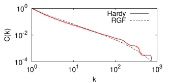
Figure 11: Size transformation of the writing by Thomas Hardy. The original data contains $M\approx 1.3\times 10^{6}$ words and is shown in figure 5. The reduced data-set contains 1% of the words and are plotted as the full-drawn line in the cumulative plot $C(k)$. This line is an average over many random removals of 99% of the words. The RGF prediction is given by the dashed line. The size transformation causes the power-law index $\gamma$ to change from $1.66$ (see figure 5) to $1.97$ when only 1% of the words remain.

More details on the RBT are given in C. The transformed Hardy has $m=1.3\times 10^{4}$, $n=3170$ and the number of ‘the’ is $k_{\max}=742$. Note that the transformations of $M$ and $k_{\max}$ are trivial: both are reduced by a factor of hundred. However, the transformation of $N$ is nontrivial: the chance of removing a specific word which occurs $k$ times in the original dataset depends in a nontrivial way on $k$. The three values $(m,n,k_{\max})$ for the transformed book give a corresponding RGF prediction for the distribution. This prediction gives $\gamma=1.9655$. Thus the prediction is that $\gamma$, because of the size transformation, increases from $1.66$ to $1.97$. This is confirmed by the actual data for the smaller dataset since the RGF prediction again gives a very good representation of the data. However, there are some small deviations. These small deviations are also reflected in a small difference of the entropy for the transformed data and the RGF prediction: The reduced data given by the full-drawn curve in figure 11 corresponds to $S=1.49064$, while the RGF prediction corresponds to $S=1.64776$. This means that the process of randomly removing words imposes some further tiny constraint in addition to what is absorbed into the RGF prediction. One should note that, from a system-specific perspective, these small deviations from the RGF are really the interesting thing, because they do reflect something system-specific. In the present case, the additional constraint is a consequence of randomly removing data. However, the most striking thing is how well the RGF describes the transformation: the removal 99% of the words is really a substantial reduction.

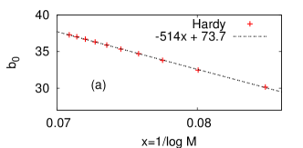
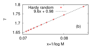
Figure 12: Systematic text-length dependence for the writings by Thomas Hardy. The data is the same as in figure 5. The average $\left<k\right>$ as a function of text length $M$ is obtained by randomly transforming the data down to a given length. Since the transformation of $k_{\max}$ is trivial, the knowledge of $\left<k\right>$ suffices for obtaining the RGF prediction. (a) and (b) show that the RGF parameters $b_{0}$ and $\gamma$ are both to good approximation linear functions of $1/\ln M$. This makes it possible to extrapolate to $M\rightarrow\infty$. The extrapolated value of $\gamma$ in the limit $M\rightarrow\infty$ is in this case $\gamma\approx 1$.

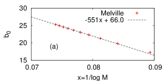
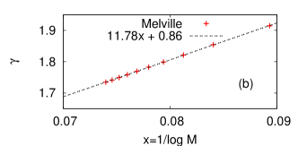
Figure 13: Systematic text-length dependence for the writings by Herman Melville. The data is the same as in figure 6. The average $\left<k\right>$ as a function of text length $M$ is obtained by randomly transforming the data down to a given length. Since the transformation of $k_{\max}$ is trivial, the knowledge of $\left<k\right>$ suffices for obtaining the RGF prediction. (a) and (b) show that the RGF parameters $b_{0}$ and $\gamma$ are both to good approximation linear functions of $1/\ln M$. This makes it possible to extrapolate to $M\rightarrow\infty$. The extrapolated value of $\gamma$ is $\gamma\approx 0.9$.

The fact that the power-law index $\gamma$ increases, when the total number of elements is reduced, also means that $\gamma$ decreases when the number of elements is increased. One may then ask if $\gamma$ acquires some special value in the limit $M\rightarrow\infty$. The fact that $\gamma$ decreases means that the effect of preferential processes diminishes, and from this perspective one might suspect that the limit value is the non-preferential value $\gamma=1$. We have tried to estimate this limit in case of the word-frequency data by Hardy and Melville: starting from the data in figure 5 and figure 6, we first transform the data to smaller sizes, by randomly removing words, and obtain the $\gamma$ and $b$ for the corresponding RGF. These are plotted as $\gamma$ versus $1/\ln M$ and $b/M$ versus $1/\ln M$ in figure 12 and figure 13 for the data from Hardy and Melville, respectively. The reason why $b_{0}\equiv b/M$ is a natural variable is explained in C. As seen in figure 12 and figure 13 for Hardy and Melville, the two quantities $\gamma$ and $b_{0}$ scale linearly with $1/\ln M$ to a very good approximation. From this, the limit value of $\gamma$ can be directly estimated: for Hardy, the value $\gamma\approx 1$ is obtained in the limit $M\rightarrow\infty$ and for Melville $\gamma\approx 0.9$. This shows that $\gamma$ does indeed decrease in a systematic way with increasing size and, furthermore, that the limit value comes close to the non-preferential value $\gamma=1$.

We note in passing that in case of a novel written by an author, one may ask how $\gamma$ changes if one analyzes a small part of the text within the novel. As shown in Ref. [19], the result is very similar to the random removal of words because, to very good approximation, the chance that a picked word belongs to the frequency class $k$ is on the average independent of the position in the book.

5 Relation to Growth Models

Most earlier attempts to explain the broad distributions for word frequencies, towns and family names are based on growth models [10, 13, 14, 25, 20]. The basic goal of these attempts focuses on explaining why the data follows a power law with an exponent close to 2. As seen from the data in section 2, such a power law does rarely give a good description of the data: the data only approximately follows a power law for small $k$ and the power-law exponent is usually significantly smaller than 2. Furthermore, these attempts completely miss the fact that, as shown here, the number of members of the largest group determines the power-law index of the power law which approximately describes the data for small $k$. However, the growth models are also problematic for two conceptual reasons. The first is that a real growth model is history-dependent. This is problematic because history and memory are usually system-specific features and any description which contains such features is less ubiquitous. The second is the relation between growth, steady state, and maximum entropy which makes the definition of a growth model rather flexible.

In order to make the connection between the RGF and growth models, we first construct a dynamical model which directly leads to the maximum-entropy solution of the equal-address-probability RGF given by (1). A simple dynamical model which achieves this is the following: start with $N$ boxes and $M$ balls and the condition that all boxes must always contain at least one ball. Then, at each time step, you pick two balls randomly with equal probability and move one of the balls to the same box as the other. Any move which attempts to empty a box is abandoned. This dynamical update has the $P(k)\propto\exp(-bk)/k$ distribution given by (1) as its steady state solution [26]. Next imagine that you watch this dynamical process from the vantage point of a single box. This box will then have a fluctuating number, $k$, of balls between 1 and $M$ following a trajectory in time $k(t)$. Since the maximum entropy dynamics is completely ergodic, it follows that $\frac{1}{t_{\max}-t_{1}}\sum_{t_{1}}^{t_{\max}}k(t_{i})$ $=\left<k\right>$ for $t_{\max}\rightarrow\infty$ and furthermore that $\frac{1}{t_{\max}-t_{1}}\sum_{t_{1}}^{t_{\max}}\delta_{k(t_{i}),k}\sim P(k)$ for $t_{\max}\rightarrow\infty$.

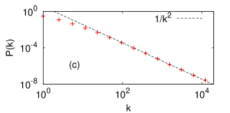
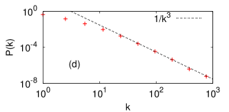
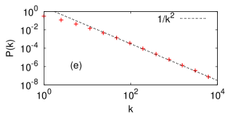
Figure 14: (a) Numerical simulation of the discretized version of the Gibrat model. The outcome of the growth is measure at a fixed time $t$ after start and the average of many such outcomes gives $P(k)$. The distribution $P(k)$ is close to log-normal. The parameters chosen are $\beta=10k/9$ and $\alpha=9k/10$. (b) The same model with the same parameters but with the restriction that the number of balls in the box cannot exceed $M$. This turns the model into an ergodic model with the steady-state distribution given by $P(k)\propto 1/k$. (c) Every $k$ can change by $\pm 0.1k$. At this point the model ceases to be a growth model and $P(k)\propto 1/k^{2}$ (d) Every $k$ can change by $+0.089k$ or $-0.1k$. This is an ergodic non-growing model and $P(k)\propto 1/k^{\gamma}$ with $\gamma\approx 3$ (e) The same parameter as in (a) and (b), but every time one subtracts a number of balls corresponding to the average increase, i.e., $\frac{1}{2}(\alpha-\beta)k$. In this way, the stochastic part of the model is turned into the non-growing Gibrat model given in (c) with the same distribution $P(k)\propto 1/k^{2}$.

Does there exist a corresponding single box stochastic process which yields the same $P(k)$ as the maximum-entropy dynamical process described above? A particular class of stochastic models are the stochastic growth models, where the box on the average grows proportional to the size of the box. The generic type can be described as follows: start with one ball in the box. Then at each time step, with probability 1/2 you either increase the box by adding $(\alpha-1)k$ balls or you subtract $(1-\beta)k$ balls, where $\alpha\geq 1$ and $\beta\leq 1$. The precise meaning is that you pick the balls in the box consecutively and with chance $(\alpha-1)$ you add an additional ball and similarly for the subtraction. The boundary condition is that the box has at least one ball. Thus if $(1-\beta)k$ is too large to be compatible with the boundary condition, you only remove all balls but one. At each time step, the box increases on the average with $\frac{1}{2}(\alpha-\beta)k$ balls. This is a generic discretized model for growth proportional to the box size. This model is in the continuum limit called the Gibrat model and the corresponding $P(k)$ has a log-normal distribution which is distinct from a power law. Figure 14 shows the average $P(k,t)$ for the discretized model for the values $\alpha=10/9$ and $\beta=9/10$ and $t=10$. This is clearly not a power law but is close to a log-normal distribution. Comparing this to the word-frequency data in figure 5 and figure 6 shows that the log-normal distribution produced by the stochastic growth model does not match the data. Consequently, growth models producing log-normal distributions are not contenders for an ubiquitous explanation of the “fat tailed” distributions presented in section 2.

The model can be turned into an ergodic version by imposing a maximal size $M$; any attempt to increase the box beyond this size is abandoned and a new attempt is made at this time step. This is just like having a fixed number of balls which you try to put into the box. The balls which are not in the box are outside on the table and you choose randomly from them when adding balls to the box. Every time you remove balls from the box you put them together with the ones on the table. Figure 14(b) shows that the stochastic steady state is $P(k)\sim 1/k$. This means that a model, which grows proportional to the box size at the same time obeys the condition $\alpha\cdot\beta=1$, has a steady-state version which corresponds to the maximum-entropy solution. This is just saying that also for the steady-state single-box-growth model, the chance of finding a specific ball in the box when it has size $k$ is independent of $k$. The reason for this can be traced to the particular stochastic update which in a logarithmic scale corresponds to $\ln k-\ln\alpha\leftarrow\ln k\rightarrow\ln k+\ln\alpha$. Thus the system wanders randomly among the values $\ln k$ within the interval $[\ln 1,\ln M]$ and, since there is no preference, the probability to find the system in any of these points are equal (modulo a slight correction imposed by the boundary points), from which $P(k)\sim 1/k$ follows. Next we consider the situation when $\alpha\cdot\beta>1$ but still a growth model, so that $\alpha-\beta>0$. This means that $1/\alpha<\beta<\alpha$. In this case, the steady-state solution instead becomes $P(k)\sim 1/k^{\gamma}$ where $1<\gamma<2$. The limit case $\alpha=\beta$ is no longer a growth model, but is an equilibrium model with a well-defined non-growing average size $\left<k\right>$. In this case, the exponent is $\gamma=2$ as illustrated in figure 14(c). When $\beta>\alpha$ the generic model is a non-growing steady-state model with the solution $P(k)\sim 1/k^{\gamma}$ with $\gamma>2$ as illustrated in figure 14(d). The Gibrat model is often connected to the non-growing steady-state solution $P(k)\sim 1/k^{2}$ by changing it into a non-stochastic growing part on top of which a stochastic non-growing part is added [25]: at each time-step one subtracts the number of balls which corresponds to the average increase during one time step, i.e., $\frac{1}{2}(\alpha-\beta)k$. In this way the growing model is transformed into a steady average growth on top of which is added the stochastic model with $\alpha^{\prime}=\beta^{\prime}=\frac{1}{2}(\alpha+\beta)k$. This changes the log-normal distribution into the non-growing steady-state distribution $P(k)\sim 1/k^{2}$, as is illustrated in figure 14(e). It is interesting to note that the distribution $P(k)\sim 1/k^{2}$ has little to do with the growing proportional to the size, but is in fact associated with the corresponding equilibrium non-growing situation. Thus from a conceptual point the difference between the log-normal and the $1/k^{2}$ distributions is precisely the difference between a stochastically growing model and a stochastically non-growing steady-state solution.

It is also interesting to note that one could equally well transform the Gibrat model by instead subtracting $ck$ balls at each time step where $c>\frac{1}{2}(\alpha-\beta)$. This again yields a model consisting of a steady average growth and a stochastic non-growing part. However now the distribution becomes $P(k)\sim 1/k^{\gamma}$ with $\gamma>2$. Thus the steady-state solutions of the stochastic growth model does give rise to power laws with a wide range of power law indices, but the actual growth is not responsible for this. As illustrated in figure 14, starting from the Gibrat model with a log-normal distribution, you can, by manipulating the boundary conditions, turn it into effective steady-state solutions which are of power-law forms and can have a broad range of power-law indices. However, a general principle, of which manipulation connects to which set of real data, is lacking.

The Gibrat models are a model for size-proportional stochastic growth of an independent box. The Simon model is a model of proportional growth for interdependent boxes [10]. It is associated with suggestive descriptions like “Rich-gets-richer” models and “Preferential attachment” models [7, 8, 27, 28]. In the context of written texts the generic form can be described as follows [10]: when you write a text, you either choose a new word or you repeat one of the words you have used earlier in the text. The Simon assumption is that you with probability $\alpha$ write a new word and with probability $1-\alpha$ you repeat an old word chosen uniformly among the words already written. Within the box-and-ball model, each new word defines a new box and a word is added to an existing box in proportion to its size. The average size of a box becomes $\left<k\right>=1/\alpha$ and the distribution for large $M$ is a power law with exponent $\gamma=1+1/(1-\alpha)>2$ [10]. For the texts by Hardy and Melville presented in figure 5 and figure 6, the Simon model predicts the power-law indices $\gamma=2.02$ and $\gamma=2.04$, respectively. As seen from the figures, the Simon model fails to describe the word-frequency data. Only the data for the French communes in section 2 could be argued to be partially described by a power law with a $\gamma$ close to 2 in the region of small $k$. But since the Simon model fails for the US county data and all the other datasets in section 2, our conclusion is that the Simon model does not have the ubiquitous generality necessary to explain the “fat tail” phenomena.

The lack of generality of the Simon model is to some extent reflected in Ref. [11] by Mandelbrot’s comment that “this is a fairly reasonable assumption in the case of word frequencies, since a text is indeed generated word by word. But a national income is surely not distributed dollar by dollar”. However, the Simon model is in fact also conceptually unreasonable for texts. This is because it is a true growth model and hence forces a history dependence on the text which is incompatible with real texts [23]: since new words are added and old words repeated at each time-step, the consequence is that the words in a Simon book which occur only a few number of times in the book occurs more often at the end of the book. In a typical text, about half the words only occur once, and in the Simon book, these words are with larger probability found at the end. In a real text, the words of any frequency group are to good approximation randomly spread through the book: the history dependence of the Simon model is a too strong system dependent assumption to make it a contender for ubiquity [19].

6 Summary

“Fat tails” are common features of datasets encountered in very different contexts. The question is then, if there is a different system-specific explanation in each case, or if the “fat tails” represent an ubiquitous non-system-specific feature. In this paper, we present evidence for a ubiquitous explanation based on a Random Group Formation (RGF) phenomena. The RGF phenomena lead to an explicit prediction of the group sizes for given values of the total number of elements, groups and the number of elements in the largest group. As a consequence, the power-law index of the power law, which approximately describes the data for small $k$, is in fact determined by the size of the largest group. These predictions were tested against six large datasets for three system types, i.e., population distributions, surname distributions and word-frequency distributions. Two datasets for each type was chosen in order to be able to compare inter- and intra differences between the datasets. In addition, the datasets were chosen to be very large in order to get good statistics. The RGF prediction was found to describe the data very well in all the cases. The RGF phenomena were also found to be consistent with a systematic change in the power-law index with system size. This system-size dependence was explicitly demonstrated in case of the word-frequency distributions.

It was also pointed out that alternative attempts to explain the “fat tails” based on growth models, like the Simon model or the Gibrat model, give power-law indices larger than 2, whereas the data presented typically have smaller values. In addition, the growth models can neither explain the coupling between the largest group and the power-law index, nor the fact that the power-law index changes in a systematic way with the system size. The growth models typically give size-independent power-law indices. The problem with system-specific memory effects for growth models, like the Simon model, was also pointed out.

The present investigation leads to the conclusion that a ubiquitous explanation must account for the fact that the largest group determines the power-law index describing the small $k$ part of the distribution, as well as the fact that the power-law index in a systematic way depends on the system size. For example, a short novel written by an author has a different power-law index than a much longer novel [23].

This leaves the critical reader with two options: either one could argue that the agreements found in the present paper are purely accidental and that there is indeed no ubiquitous explanation of the “fat tails”. Or you could argue that there is a ubiquitous explanation but it is not given by the RGF. In the latter case, one would then have to come up with an alternative explanation which accounts for the fact that the size of the largest group determines the power-law index for small $k$ and which, at the same time, is consistent with a systematic size dependence.

For our part, we think that the evidence in favor of the RGF explanation is entirely convincing. Furthermore, since the RGF gives explicit predictions, its validity is open to further tests.

References

Appendix A Minimum information cost and maximum entropy

Suppose you have two variables $x$ and $y$ distributed according to the corresponding probability functions $p(x)$ and $p(y)$, respectively. The total entropy $H[p(x),p(y)]$ is then given by

$$H[p(x),p(y)]=-\sum_{x}\sum_{y}p(x,y)\ln p(x,y),$$ (8)

where $p(x,y)$ is the joint probability for the variables $x$ and $y$. If the two distributions are independent (so that the probability for a value $x$ is independent of the value $y$), then $p(x,y)$ reduces to $p(x,y)=p(x)p(y)$ and the entropy reduces to $H[p(x),p(y)]=H[p(x)]+H[p(y)]$ where $H[p(x)]=-\sum_{x}p(x)\ln p(x)$. In many situations, $p(x)$ and $p(y)$ are dependent so that $p(x,y)\neq p(x)p(y)$ or equivalently the constrained probability $p(x|y)$ (the probability for a $x$ for a fixed given $y$) is in fact not equal to $p(x)$ i.e. $p(x|y)\neq p(x)$ (note the general relation $p(x,y)=p(x|y)p(y))$. We here consider the special case when the distribution $p(y)$ is a priori known. In such a case, the maximum entropy $H[p(x)]$ is obtained by minimizing the constrained entropy

$$H[p(y)|p(x)]=-\sum_{x}\sum_{y}p(x,y)\ln p(y|x)$$ (9)

This follows from the general maximum-mutual-information principle [22]. The mutual information is defined by

$$I[p(x),p(y)]=\sum_{x}\sum_{y}p(x,y)\ln\frac{p(x,y)}{p(x)p(y)}$$ (10)

and the $p(x)$ corresponding to maximum entropy is obtained by maximizing the mutual information for the given $p(y)$. However, the mutual information can also be expressed as $H[p(y)|p(x)]=-I[p(x),p(y)]+H[p(y)]$ and since $p(y)$ is a priori known it follows that maximizing $I[p(x),p(y)]$ is equivalent to minimizing the constrained entropy $H[p(y),p(x)]$. This constrained entropy we term the information cost $I_{\rm cost}[p(x)]=H[p(y),p(x)]$. In the case of the equal-address RGF, the information cost is given by

$$I_{\rm cost}[P(k)]=H[p_{i}|P(k)]=-\sum_{k}\sum_{i}p(k,i)\ln p(i|k)$$ (11)

The a priori known distribution is the equal probability for each of the $M$ addresses, so that $p_{i}=\frac{1}{M}$. This means that $p(i|k)=\frac{\delta_{k^{\prime}(i),k}}{kN(k)}$ and consequently $p(i,k)=\frac{\delta_{k^{\prime}(i),k}}{kN}$. Inserting this in (11) gives

$$I_{\rm cost} = -\sum_{k}\sum_{i}p(k,i)\ln p(i|k)=-\sum_{k}P(k)\ln\frac{1}{kN(k)}$$ (12)

$$= \sum_{k}P(k)\ln kN(k)$$

The conceptual advantage with the quantity $I_{\rm cost}$ is that it has a simple interpretation: if you know that a specific ball can be found among the boxes which contain $k$ balls, then $\ln kN(k)$ is the information (in nats) needed to specify at which specific address the ball can be found. The average information cost needed for localizing a ball with a known $k$-value is hence $I_{\rm cost}=\sum_{k}P(k)\ln kN(k)$.

This is an information cost in the sense that the additional info needed to specify the outcome of the $p(i)$ is no longer available for the entropy associated with $P(k)$.

Appendix B Self-consistent Equations

The RGF-curve is obtained by minimizing the total information cost $G[P(k)]$ given by (3). The minimum condition $\frac{\partial G([P(k)]}{\partial P(k)}=0$ leads to the condition

$$\ln P(k)+\ln k+1+c_{1}+c_{2}k-c_{3}\ln P(k)-c_{3}=0$$ (13)

with the solution given in (4)

$$P(k)=A\frac{\exp(-bk)}{k^{\gamma}}$$ (14)

with $\gamma=1/(1-c_{3})$, $b=c_{2}/(1-c_{3})$ and $A=\exp\{-(1+[c_{1}/(1-c_{3})]\}$. The constants $A$, $b$ and $\gamma$ are determined by simultaneously fulfilling three conditions. The first two of these conditions are $\sum_{k=k_{0}}^{M}P(k)=1$ and $\sum_{k=k_{0}}^{M}kP(k)=\left<k\right>=M/N$, i.e.,

$$\left\{\begin{array}[]{l}\sum_{k=k_{0}}^{M}A\frac{e^{-bk}}{k^{\gamma}}=1\\ \sum_{k=k_{0}}^{\infty}Ak\frac{e^{-bk}}{k^{\gamma}}=M/N\end{array}\right.$$ (15)

where $k_{0}$ is the size of the smallest box. The natural limit is $k_{0}=1$, but can equally well be generalized to an arbitrary $k_{0}$. This means that the constants $\gamma$ and $b$ are interdependent through the relation

$$\frac{\sum_{k=k_{0}}^{M}\frac{e^{-bk}}{k^{\gamma-1}}}{\sum_{k=k_{0}}^{M}\frac{e^{-bk}}{k^{\gamma}}}=\frac{M}{N}.$$ (16)

The third condition is determined by requiring a specific average value for the size of the largest box $\left<k_{\max}\right>$. In the direct comparison with a single dataset, this value is approximated with the actual value of $k_{\max}$ for the dataset. The calculation of $\left<k_{max}\right>$ is made in two steps: first a value $k_{c}$ is determined by the condition that $\sum_{k=k_{c}}^{M}P(k)=1/N$. This means that on the average there is precisely one box in the interval $[k_{c},M]$. The second step is to calculate the average size of a box in the interval $[k_{c},M]$, i.e.,

$$\left<k_{\max}\right>=\frac{\sum_{k=k_{c}}^{\infty}kP(k)}{\sum_{k=k_{c}}^{\infty}P(k)}.$$ (17)

Thus the three requirements turn into a set of self-consistent equations: one starts by assuming a certain value for $\gamma$ and then one obtains $b$ by using (16). Thus the two basic constraints (15) yields $P(k)$ from the trial $\gamma$. Next this trial $P(k)$ is inserted in (17). If (17) is not satisfied within a predefined precision, we repeat this procedure with a new trial $\gamma$. In this way, the correct values of $A$, $b$ and $\gamma$ can be self-consistently determined.

Appendix C Random Book Transformation

Suppose we want the distribution for an $n$th part of a book which has the word-frequency distribution $P(k)$. The chance that a picked word is part of the $n$th part is $\frac{1}{n}$ and the chance that it is not is $\frac{n-1}{n}$. Consequently the RBT gives [19, 23, 24]

$$P_{\frac{1}{n}}(k)=\frac{\sum_{k^{\prime}=k}\left(\frac{1}{n-1}\right)^{k}(\frac{n-1}{n})^{k^{\prime}}\left(\begin{array}[]{c}k^{\prime}\\ k\end{array}\right)P(k^{\prime})}{1-\sum_{k^{\prime}=1}(\frac{n-1}{n})^{k^{\prime}}P(k^{\prime})}$$

where $\left(\begin{array}[]{c}k^{\prime}\\ k\end{array}\right)$ is the binomial coefficient and the normalization is appropriate because

$$\sum_{k=1}P_{\frac{1}{n}}(k) = \frac{1}{1-P_{\frac{1}{n}}(0)}\sum_{k^{\prime}=1}\left(\frac{n-1}{n}\right)^{k^{\prime}}P(k^{\prime})\sum_{k=1}^{k^{\prime}}\left(\frac{1}{n-1}\right)^{k}\left(\begin{array}[]{c}k^{\prime}\\ k\end{array}\right)$$

$$= \frac{1}{1-P_{\frac{1}{n}}(0)}\sum_{k^{\prime}=1}\left(\frac{n-1}{n}\right)^{k^{\prime}}P(k^{\prime})\left[\left(\frac{n}{n-1}\right)^{k^{\prime}}-1\right]$$

$$= \frac{1}{1-P_{\frac{1}{n}}(0)}\left[1-P_{\frac{1}{n}}(0)\right]=1$$

The RBT can be analytically obtained in two limiting cases. These are the equal-address RGF distribution $P(k)\propto\exp(-bk)/k$ and the limit distribution $P(k)\propto\exp(-bk)/\left[k(k-1)\right]$. The transformed solution in the first case is given by

$$P_{\frac{1}{n}}(k)\propto\frac{\exp\{-k\ln[n(e^{b}-1)+1]\}}{k}$$

and, since $(e^{b}-1)=b$ for small $b$, it reduces to

$$P_{\frac{1}{n}}(k)\propto\frac{\exp[-k\ln(nb+1)]}{k}\propto\frac{\exp(-knb)}{k}.$$

This means that the exponential cutoff increases linearly with $n=M/m$, or in other words, the size dependence is to good approximation given by $P_{m}(k)\propto\frac{\exp(-kb_{0}/m)}{k}$ where $b_{0}$ is a constant. This result just reflects the fact that the exponential cuts off the distribution at the system size $m$. An important consequence is that the functional form $P(k)\propto 1/k$ is invariant under the RBT. This is a very special property and $P(k)\propto 1/k$ is presumably the only nontrivial invariant functional form with a finite value at $k=1$. The typical situation is that the shape of $P(k)$ becomes less broad under the transformation, e.g., $P(k)\propto 1/k^{\gamma}$ with $\gamma>1$ will have an increasing $\gamma$ with decreasing size.

The functional form $P(k)\propto\exp(-bk)/[k(k-1)]$ transforms as

$$P_{\frac{1}{n}}(k) \propto \frac{1}{k(k-1)}\times\frac{1}{n}\times\frac{1}{(e^{b}n-n+1)^{k-1}}$$ (19)

$$\propto \frac{\exp(-bnk)}{k(k-1)}.$$

One notes that the exponent transforms in the same way and has the form $\exp(-kb_{0}/m)$. One also notes that the form $P(k)\propto 1/[k(k-1)]$ is invariant but that it is infinite for $k=1$. The point is that if you start from $P(k)\propto 1/k^{\gamma}$ then the transformed $P_{m}(k)$ approaches the limit form $P_{\infty}(k)\propto 1/[k(k-1)]$. It is also interesting to note that, for $k$ values not too small, the limiting function is a power law with exponent $\gamma=2$.

One may then ask what happens if we instead followed the transformation in the reverse direction towards larger books. Since $P(k)\propto 1/k$ is invariant under the transformation, it seems likely that it is also the limiting function in the reverse direction so that $P_{0}(k)\propto 1/k$. This suggests that a book approaches this word-frequency distribution in the limit of infinite size. As seen from the data analysis in section 4, this expectation seems to have some support in the actual data. One may perhaps also speculate that since $\gamma=1$ for the upper limit and $\gamma=2$ for the lower, it should not be a surprise that $\gamma$ values within $1<\gamma<2$ are often found in real data.

References

- [1] V. Pareto. Cours d’Economie Politique. Droz, Geneva, 1896.
- [2] F. Auerbach. Das Gesetz der Bevolkerungskonzentration. Petermanns Geographische Mitteilungen, 59, 1913.
- [3] G. Zipf. Selective studies and the principle of relative frequency in language. Harvard University Press, Cambridge, Massachusetts, 1932.
- [4] G. Zipf. The psycho-biology of language: An introduction to dynamic philology. Mifflin Company, Boston, Massachusetts, 1935.
- [5] G. Zipf. Human bevavior and the principle of least effort. Addison-Wesley, Reading, Massachusetts, 1949.
- [6] J. B. Estroup. Gammes Sténographiques. Institut Stenographique de France, Paris, 4 edition, 1916.
- [7] M. Mitzenmacher. A brief history of generative models for power law and lognormal distributions. Internet Mathematics, 1:226, 2003.
- [8] M. E. J. Newman. Power laws, pareto distributions and zipf’s law. Contemporary Physics, 46:323, 2005.
- [9] A. Clauset, C. R. Shalizi, and M. E. J. Newman. Power-law distributions in empirical data. SIAM Review, 51:661–703, 2009.
- [10] H. Simon. On a class of skew distribution functions. Biometrika, 42:425, 1955.
- [11] B. Mandelbrot. A note on a class of skew distribution functions: Analysis and critique of a paper by H. A. Simon. Information and Controll, 2:90, 1959.
- [12] B. Mandelbrot. An informational theory of the statistical structure of languages. Butterworth, Woburn, Massachusetts, 1953.
- [13] R. Gibrat. Une loi des réparations économiques: l’effet proportionnel. Bull. Statist. gén Fr., 19:469, 1930.
- [14] R. Gibrat. Les inegalites economiques. Libraire du Recueil Sirey, Paris, 1931.
- [15] http://www.census.gov/population/www/cen2000/briefs/phc-t4/index.html.
- [16] http://www.citypopulation.de/France.html.
- [17] http://www.census.gov/genealogy/www/data/2000surnames/index.html.
- [18] http://en.wikipedia.org/wiki/ListofKoreanfamilynames.
- [19] S. Bernhardsson, L. E. C. da Rocha, and P. Minnhagen. The meta book and size-dependent properties of written language. New J. Phys., 11:123015, 2009.
- [20] D. H. Zanette and S. C. Marunbia. Vertical transmission of culture and the distribution of family names. Physica A, 295:1, 2001.
- [21] S. K. Baek, H. A. T. Kiet, and B. J. Kim. Family name distributions: Master equation approach. Phys. Rev. E, 76:046113, 2007.
- [22] T. M. Cover and A. T. Joy. Elements of Information Theory. Wiley, Hoboken, New Jersey, 2 edition, 2006.
- [23] S. Bernhardsson, L. E. C. da Rocha, and P. Minnhagen. Size dependent word frequencies and the translational invariance of books. Physica A, 389:330, 2010.
- [24] R. H. Baayen. Word frequency distributions. Kluwer Academic Publisher, Dordrecht, The Netherlands, 2001.
- [25] X. Gabaix. Zipfś law for cities: An explanation. Quarterly Journal of Economics, 114:739, 1999.
- [26] P. Minnhagen, S. Bernhardsson, and B. J. Kim. Scale-freeness for networks as a degenerate ground state: A Hamiltonian formulation. EPL, 78:28004, 2007.
- [27] A.-L. Barabási, R. Albert, and H. Jeong. Emergence of scaling in random networks. Science, 286:509, 1999.
- [28] M. Newman, A.-L. Barabási, and D. Watts. The Structure and Dynamics of Networks. Princeton University Press, Princeton and Oxford, 2006.