The Velocity Field Around Groups of Galaxies

Abstract

A statistical method is presented for determining the velocity field in the immediate vicinity of groups of galaxies using only positional and redshift information with the goal of studying the perturbation of the Hubble flow around groups more distant than the Local Group. The velocities are assumed to obey a Hubble-like expansion law, i.e. $V=H_{exp}R$ where the expansion rate $H_{exp}$ is to be determined. The method is applied to a large, representative group catalog and evidence is found for a sub-Hubble expansion rate within two well defined radii beyond the virial radii of the groups. This result is consistent with that of Teerikorpi et al. (2008) who found a similar expansion law around 3 nearby groups and extends it to a more representative volume of space.

1 Introduction

Teerikorpi et al. (2008) (hereafter T08) have recently shown that galaxies in the immediate vicinity of 3 nearby groups of galaxies exhibit a Hubble-like expansion law at a slightly sub-Hubble expansion rate. The authors had at their disposal measured velocities and distances in order to arrive at this result. T08 interpret their result in terms of the effects of dark energy. The arguments for the dark energy interpretation can be found in a series of papers starting with Chernin et al. (2000). Briefly, when a density perturbation which is to become a galaxy group collapses, it leaves behind an empty annulus between the original turn-around radius designated here $R_{ES}$, and its post-collapse zero-velocity radius which lies between the virial radius and $R_{v}$. $R_{v}$ is the radius where the gravity force of the group mass is balanced by the antigravity force of the vacuum energy. Should a galaxy find itself in the region between $R_{v}$ and $R_{ES}$ either as a result of the chaos of virialization or by later ejection from the group, it may be accelerated by the effects of the vacuum energy. Since as these authors argue, the radial motion of the particles within this shell should be nearly the same as Newtonian motion its expansion velocity can be described by the vacuum Hubble constant $H_{v}=\sqrt{\Omega_{\Lambda}}H_{o}$. Maccio et al.(2005) found from N-body simulations that the observed coldness of the local Hubble flow around the local group is consistent with the dark energy interpretation.

However recently Hoffman et al. (2008) and Martinez-Vaquero et al. (2009) using sophisticated cosmological simulations claim that dark energy should have no effect on the local dynamics. In particular, these authors showed that a similar local Hubble flow was also found in an open cosmological model making the need for a $\Lambda$ model unnecessary locally. Further, Sandage (1986) has shown analytically that sub-Hubble flows can exist around groups in cosmologies without a $\Lambda$ term though of a different form from that found by T08. It is clearly of interest to confirm and extend the T08 result. In order to do so a new method for finding the velocity field is required since with increasing distances the only observational data available are positions and redshifts both for the groups and the field galaxies. The goal here is to devise such a method and to apply it to an existing group catalog in order to determine if the perturbations to the Hubble expansion law found by T08 apply to groups in a larger and more representative volume of space.

2 Fitting the Velocity Field Around Galaxy Groups with a Hubble-like Expansion Law

Determining the expansion velocity in terms of Hubble-like law ($V=H_{exp}R$) requires knowledge of the velocity with respect to the group center in the direction of expansion $V$, and the distance from the group center $R$. To demonstrate the essence of the method, assume for the moment that two projections of this expansion law are available (i.e. $\Delta V=Vcos(\theta)$ and $\Delta R=Rsin(\theta)$ in Fig 1 ). Let $y^{\prime}=V~{}cos(\theta)$ and $x^{\prime}=H_{exp}R~{}sin(\theta)$. Then

$$y^{\prime}/x^{\prime}=\frac{V}{H_{exp}R}cos(\theta)/sin(\theta)$$ (1)

Now take the average of both sides of this equation assuming that the number of groups is large and that the surrounding field galaxies are randomly distributed about these groups and denote the mean of the angular term as

$$I_{n}=\frac{1}{4\pi}\int_{sphere}cos(\theta)/sin(\theta)d\omega$$ (2)

after rearranging terms $H_{exp}$ is varied until the ratio

$$\overline{(y^{\prime}/x^{\prime})}/I_{n}=1=\overline{V/H_{exp}R}$$ (3)

and the true expansion rate is obtained. In practice, instead of $V~{}cos(\theta)$ and $R~{}sin(\theta)$ which are not known, we do have access to the components $V~{}cos(\beta)$ and $R~{}sin(\beta)$ (Fig.1) so an intermediate step is required and is described below.

The observational data available consists of the angular positions and redshifts of the group centers and the field galaxies ($z_{g}$ and $z_{f}$). For a given cosmology, co-moving distances d(z) can be calculated from $d(z)=c/H_{o}\int_{0}^{z}dz^{\prime}/((1-\Omega_{\Lambda})(1+z^{\prime})^{3}+\Omega_{\Lambda})^{1/2}$. Note that $\Omega_{k}=0$ is assumed allowing the use of Euclidean geometry. Further the redshifts of all the data to be analysed are $\lesssim 0.1$ so that the changes due to different assumed cosmologies are small. From Fig.1 with $d_{g}$ now available

$$r_{p}=R~{}sin(\beta)=d_{g}sin(\alpha)$$ (4)

and

$$d_{per}=d_{g}cos(\alpha)$$ (5)

Numerically inverting the above expression for co-moving distance allows the calculation of $z_{per}$, the redshift at $d_{per}$.

Now consider the line of sight projection of the expansion law $\Delta V_{D}$ where

$$\Delta V_{D}=V~{}cos(\beta)\simeq c(z_{f}-z_{per})$$ (6)

and define the ratio $y/x$ as follows

$$y/x=\Delta V_{D}/(r_{p}~{}H_{exp})=(V/H_{exp}R)cos(\beta)/sin(\beta)$$ (7)

Rotate the line-of-sight about the observer by $+~{}\alpha$ and define a new ratio in terms of $\theta=\alpha+\beta$. Since $V$ and $R$ remain unchanged by this operation we obtain

$$y^{\prime}/x^{\prime}=\mid(-sin(\alpha)+(y/x)cos(\alpha))/(cos(\alpha)+(y/x)sin(\alpha))\mid=(V/H_{exp}R)\mid cos(\theta)/sin(\theta)\mid$$ (8)

Note that by taking the absolute value in (8) the integral over the sphere becomes by symmetry

$$I_{n}=\frac{2\pi\int_{0}^{\pi/2}\mid(cos(\theta)/sin(\theta))\mid sin(\theta)d\theta}{2\pi\int_{0}^{\pi/2}sin(\theta)d\theta}=1$$ (9)

Hence

$$\overline{V/H_{exp}R}=\overline{y^{\prime}/x^{\prime}}$$ (10)

where the true value of $H_{exp}$ is that which makes the right hand side of (10) equal to unity. For convenience we shall refer to the statistic represented by (10) as $Y(H_{exp})$. Lastly from Fig 1 and equation (7)

$$R(H_{exp})=r_{p}/sin(\beta)=r_{p}/sin(cot^{-1}(\Delta V_{D}/(r_{p}H_{exp})))$$ (11)

where $H_{exp}$ is the value obtained above.

The above analysis applies to any one region undergoing Hubble-like expansion at a rate $H_{exp}$.

The region with the sub-Hubble expansion rate ($H_{v}$) found by T08 lies between $R_{v}$ and $R_{ES}$ in Fig.1. ($R_{v}$, $R_{ES}$ and $H_{v}$ are defined in the next section). Beyond $R_{ES}$ the expansion is assumed to return to the global Hubble rate $H_{o}$ ($H(z)$). (At higher $z$ the global rate becomes $H(z)=H_{o}((1-\Omega_{\Lambda})(1+z)^{3}+\Omega_{\Lambda})^{1/2}$). Similarly, by (11) in each of these regions we then have $R(H_{v})$ and $R(H(z_{g}))$.

With two expanding regions, the four key quantities in the analysis are the mean of the ratio $y^{\prime}/x^{\prime}$ (equ’n 10) evaluated with $H_{v}$ and $H(z_{g})$ replacing $H_{exp}$ designated here $Y(H_{v})$ and $Y(H(z_{g}))$ and the normalized distances $R(H_{v})/R_{v}$ and $R(H(z_{g}))/R_{v}$. These four quantities are calculated for every field galaxy. In order to confirm the T08 result, $Y(H_{v})$ should be unity when $1\leq R(H_{v})/R_{v}\leq R_{ES}/R_{v}$ for the particular value of $H_{exp}=H_{v}$ and $Y(H(z_{g}))$ should be unity when $R(H(z_{g}))/R_{v}$ becomes larger than $R_{ES}/R_{v}$. Both of the above conditions rely on the assumption that the galaxies are randomly distributed about the group centers for the sample as a whole. Note also that because we are dealing with ratios, the result is independent of the actual value assumed for $H_{o}$.

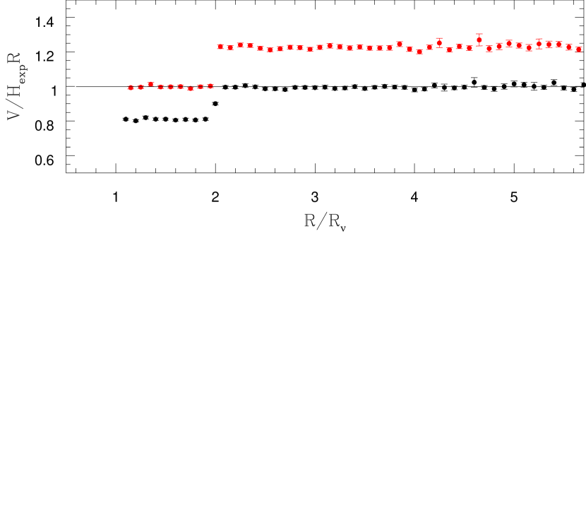
In order to validate the above procedure a simple numerical simulation was performed. In this simulation the same group properties i.e. the positions, redshifts and masses (from which $R_{v}$ could be calculated) of groups used in the analysis of the observations were used as centers around which ‘field galaxies’ were randomly distributed (both in angle $\theta$ and group-centric distance $R$). Around each of the 12620 group centers are 300 randomly chosen field galaxies. For a given cosmology, line-of-sight redshifts were assigned (either as a result of global Hubble expansion or sub- Hubble expansion about the group center) depending on whether $R/R_{v}$ was greater than or less than 2. The simulation is clearly idealized to the extent that each group and its retinue of randomly distributed galaxies was treated as an isolated system. The data were then analysed (as described above) using the same routines that were used for the observations. Here the values of $R$ plotted on the abscissa come from the simulation. Shown in Fig. 2 are the results for an assumed ($\Omega_{m},\Omega_{\Lambda},\Omega_{k}$) (0.3,0.7 ,0.0) cosmology. The red points represent $Y(H_{v})$ and $R/R_{v}$. The black points were calculated assuming $H_{exp}=H(z_{g})$ and plotted as $Y(H(z_{g}))$ versus $R/R_{v}$. Note the characteristic step in the distribution of both sets of points at the transition point ($R/R_{v}=2$) and the continuity of red and black points at $\overline{V/H_{exp}R}=1$.

3 Analysis of the Observations

3.1 The Data

The Tago et al. (2006) group catalogue of galaxies from the 2DF redshift survey (Colless et al. 2001, 2003) consists of 3 tables-one enumerates the groups and their properties, the second lists the group members while the third gives the co-moving distances of the galaxies which do not belong to any group. This catalogue was constructed using a friends-of friends algorithm. As such any individual group is subject to contamination problems (e.g. Niemi & Valtonen 2009). In the application discussed here, the groups are used statistically so that any contamination effects will affect the determination of both sub-Hubble and the global Hubble rate in the same way. For this investigation we limited our selection of groups to those lying within 300/h Mpc. This sample contains 12620 groups. The virial theorem (i.e. $M=(\pi/2)r_{virial}3\sigma^{2}/G$) where $r_{virial}$ and $\sigma$ are given in the first table of the group catalog was used to determine the mass of each of the groups. These masses were then used to calculate values of $R_{v}$ from equation (12) below.

For a given group each field galaxy subtends an angle $\alpha$ between it and the group center and each lies at the tabulated co-moving distance computed for a ($\Omega_{m},\Omega_{\Lambda},\Omega_{k}$) (0.3,0.7,0.0) with $H_{o}=100h$ and $h=1$ cosmology. These data are used to recover the individual redshifts ($z_{g}$ and $z_{f}$) which the authors had corrected for the motion relative to the CMB. The redshifts are then used to recompute the co-moving distances $d_{g}$ and $d_{f}$ (now assuming h=0.7) for the different trial cosmologies considered below.

3.2 Some Definitions

For the purpose of comparing the velocity field derived here with that of T08, we define the following analogous quantities.

Let $M$ represent the mass of an individual group and define the two radii $R_{v}$, and $R_{ES}$ as follows.

$$M/(4\pi R_{v}^{3}/3)=2\rho_{v}=2\Omega_{\Lambda}\rho_{c}$$ (12)

and

$$M/(4\pi R_{ES}^{3}/3)=\rho_{m}=(1-\Omega_{\Lambda})\rho_{c}$$ (13)

here $\rho_{c}$ is the critical density and is equal to $3H_{o}^{2}/8\pi G$. $R_{v}$ is the radius where the gravity force of mass M is balanced by the antigravity force of the dark energy . $R_{ES}$ is the radius within which the the mass now in the group originated and beyond which the velocity field approaches the global Hubble flow (Teerikorpi & Chernin, 2010 hereafter T10). Note that $R_{ES}/R_{v}=(2\Omega_{\Lambda}/(1-\Omega_{\Lambda}))^{1/3}$ and is greater than one as long as $\Omega_{\Lambda}>1/3$. The region within $R_{ES}$ is referred to by T08 as an Einstein-Straus vacuole. Also recall that $M/(4\pi R_{virial}^{3}/3)\sim 200\rho_{c}$ so that $R_{v}/R_{virial}\sim 5.1$. Rearranging (12)

$$R_{v}=(GM/(H_{o}^{2}\Omega_{\Lambda}))^{1/3}$$ (14)

Finally we parameterize the unknown sub-Hubble expansion rate as

$$H_{v}=\sqrt{\Omega_{\Lambda}}H_{o}$$ (15)

where following T08 we have neglected higher order terms (Chernin et al., 2000). This expression (referred to as the vacuum Hubble constant) also follows from the first Friedmann equation with $\Omega_{m}$ and $\Omega_{k}$ set to zero and is independent of redshift.

Before presenting the observations, we discuss some limitations of the method imposed by the observations themselves. Velocity components along the line of sight beyond the projection of the actual expansion velocity will bias our statistic to be larger than one. Two contributors are redshift errors and peculiar motions (a ‘noisy’ Hubble flow). Redshift errors are $\sim 85~{}kmsec^{-1}$ (Colless et al. 2001). The imprecise location of the group center will generally bias our statistic to be less than one. If both the inner and global expansion laws are affected in the same way the severity of the above biases can be monitored by evaluating the statistic for galaxies undergoing global Hubble expansion. Another point to consider is that groups that are close together can have the same field galaxies in common. However, just as galaxies participating in the Hubble flow are doing so irrespective of the co-moving center, the same argument applies to galaxies assumed to be expanding within the vacuum dominated region. For this reason, we choose galaxies within each region $1<R/R_{v}<R_{ES}/R_{v}$ (vacuum dominated region) and $R/R_{v}>R_{ES}/R_{v}$ (global Hubble expansion region) and treat them as separate samples.

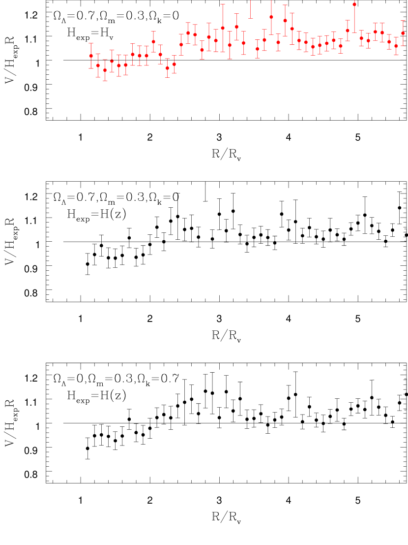
In order to determine the dividing line between sub-Hubble and global expansion, solutions were obtained for the data broken up into small groups with similar values of $R_{v}$. It was found that the distinct step pattern seen in the simulation (Fig. 2) while visible for the whole sample was most clearly defined when using only those groups with $2.6<R_{v}(h^{-1}_{70}Mpc)<3.3$ for $\Omega_{\Lambda}=0.7$. The corresponding range in group mass is $\sim 1-2\times 10^{13}h^{-1}M_{\odot}$. The results are shown in the top two panels of Fig. 3. Similar results were found for other trial values of $\Omega_{\Lambda}$ after allowing for the $\Omega_{\Lambda}$ dependence of $R_{v}$ and are shown in Fig. 5. The bottom panel of Fig. 3 shows the results of assuming an open cosmology model (OCDM) with $\Omega_{m}=0.3,\Omega_{\Lambda}=0,\Omega_{k}=0.7$ for the same groups and with the above values of $R_{v}$ used here in order to allow a comparison of results between the two cosmological models. Technically $R_{v}=\infty$ for the open model. Common to all 3 panels, the point-to-point scatter appears smaller below the break than it does above. The dispersion of the distribution of $Y(H(z_{g}))$ for 117896 group-galaxy pairs above the break (middle panel) is twice that of the dispersion of $Y(H_{v})$ for the 9894 group-galaxy pairs below the break (top panel). Comparable numbers apply to the other models shown in Fig. 5. If the galaxies below the break originated from within the group they will have the group peculiar motion imprinted on them and they will exhibit a ‘cooler’ flow. Beyond the break the galaxies are uncoupled from the groups and show the full effects of peculiar motion. This applies here to both the OCDM and $\Lambda$CDM model because the break appears in the same place. The bottom 2 panels show that the global Hubble rate cannot account for expansion velocities of the galaxies in the region below the break. The $\Lambda$CDM model can provide the appropriate sub-Hubble rate (top panel).

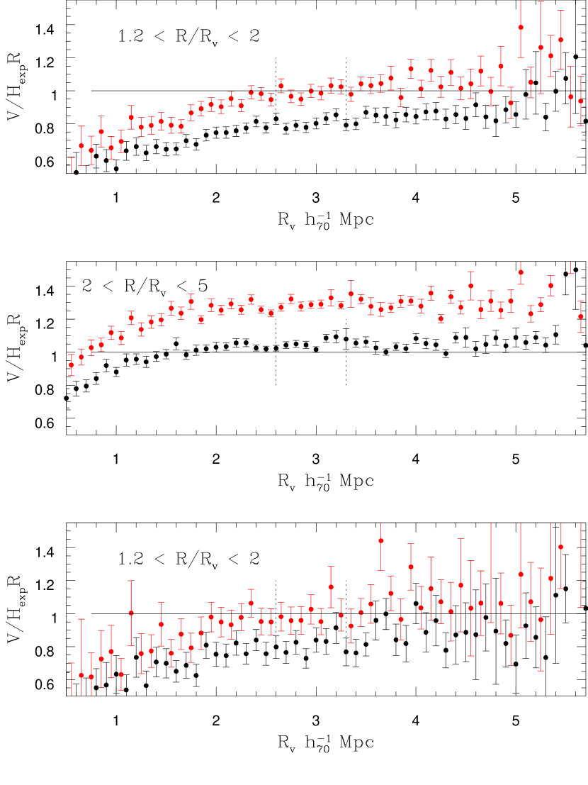
Fig. 3 shows that the dividing line between the two velocity regimes is reasonably sharp and occurs at $R/R_{v}=2.0\pm 0.1$. We identify this particular value of $R$ as $R_{ES}$. (Note from equ’ns (12) and (13) the ratio $R_{ES}/R_{v}$ is predicted to be 1.7 when $\Omega_{\Lambda}=0.7$ and 2 when $\Omega_{\Lambda}=0.8$ (T10). A possible explanation for this small discrepancy comes from the observations of galaxy clusters that a substantial amount of mass (up to $100\%$) exists outside the virial radius but within the post- collapse zero-velocity radius which is below $R_{v}$ (e.g. Rines & Diaferio 2006). Allowing for this possibility would increase $R_{v}$ by $2^{1/3}$ and the predicted ratio would be recovered). Another possible contributor to the discrepancy in $R_{ES}/R_{v}$ is our neglect of the ‘lost-gravity’ term due to dark energy in the calculation of the virial mass (Chernin et al. 2009). It is instructive to divide the data at this point and to plot the statistic (equ’n 10) versus $R_{v}$ itself. The results are shown in Fig. 4 for the case $\Omega_{\Lambda}=0.7$. The top panel shows results for $R/R_{v}<2$ for all 12577 groups with $R_{v}<5.7h^{-1}_{70}Mpc$. The middle panel shows results for the same sample for $R/R_{v}>2$. As before the red points represent the statistic calculated with $H_{exp}=H_{v}=0.84H_{o}$ (i.e. $\Omega_{\Lambda}=0.7$) while the black points were obtained with $H_{exp}=H(z_{g})$. The dotted lines enclose the region used to construct Figs. 3 & 5. The region at $R_{v}<2h^{-1}_{70}Mpc$ never reaches unity while the data become very noisy at $R_{v}>3.3h^{-1}_{70}Mpc$ and the break becomes less well defined. It is interesting that the N-body simulations of Wang et al. (2009) show (their Fig. 6) that for host halo masses greater than $10^{13}h^{-1}M_{\odot}$ ejected sub-halos fall back while for host halo masses lower than this ejected sub-halos are likely to reach the region beyond $R_{v}$. The data in this higher mass range are too sparse to determine whether this same phenomenon is responsible for the break becoming less well defined. Plots for higher and lower values of $\Omega_{\Lambda}$ are similar with the statistic among the red points between the dashed lines in the $R/R_{v}<2$ plots asymptoting at lower and higher values. The results for $R/R_{v}>2$ (black points) for a range in vacuum energy are very similar to those shown in the middle panel. It is not clear what is responsible for the fall-off below $R_{v}\sim 2h^{-1}_{70}Mpc$ in these plots especially given that T08 found their result at $R_{v}\sim 1.3h^{-1}_{70}Mpc$. A possible explanation comes from the observation that the galaxies that are supposed to be expanding at the Hubble rate (those plotted in the middle panel) also show large deviations from unity in the same low range of $R_{v}$ suggesting that the field galaxies surrounding these low mass groups may not be uniformly distributed.

A sub-sample of more isolated groups was analysed in order to measure the effect of group clustering on the result. This sub-sample included only those 3894 groups of the original 12620 without a neighbor within $4h^{-1}_{70}Mpc$. The results are shown in the bottom panel of Fig. 4 and can be compared to the top panel. The previous results shown in Figs 3 & 5 remain unchanged but with larger uncertainty. In addition the fall-off below $R_{v}\sim 2h^{-1}_{70}Mpc$ noted above is still present. This region should show the most change if the effect of clustering is a dominating influence. Increasing the isolation criterion above leaves too few groups and very poor statistics.

As a further check on the results another sub-sample consisting of only those 1835 groups with more than 5 members was analysed. These results have larger uncertainties but there are no systematic differences from those shown in Figs 3 & 4.

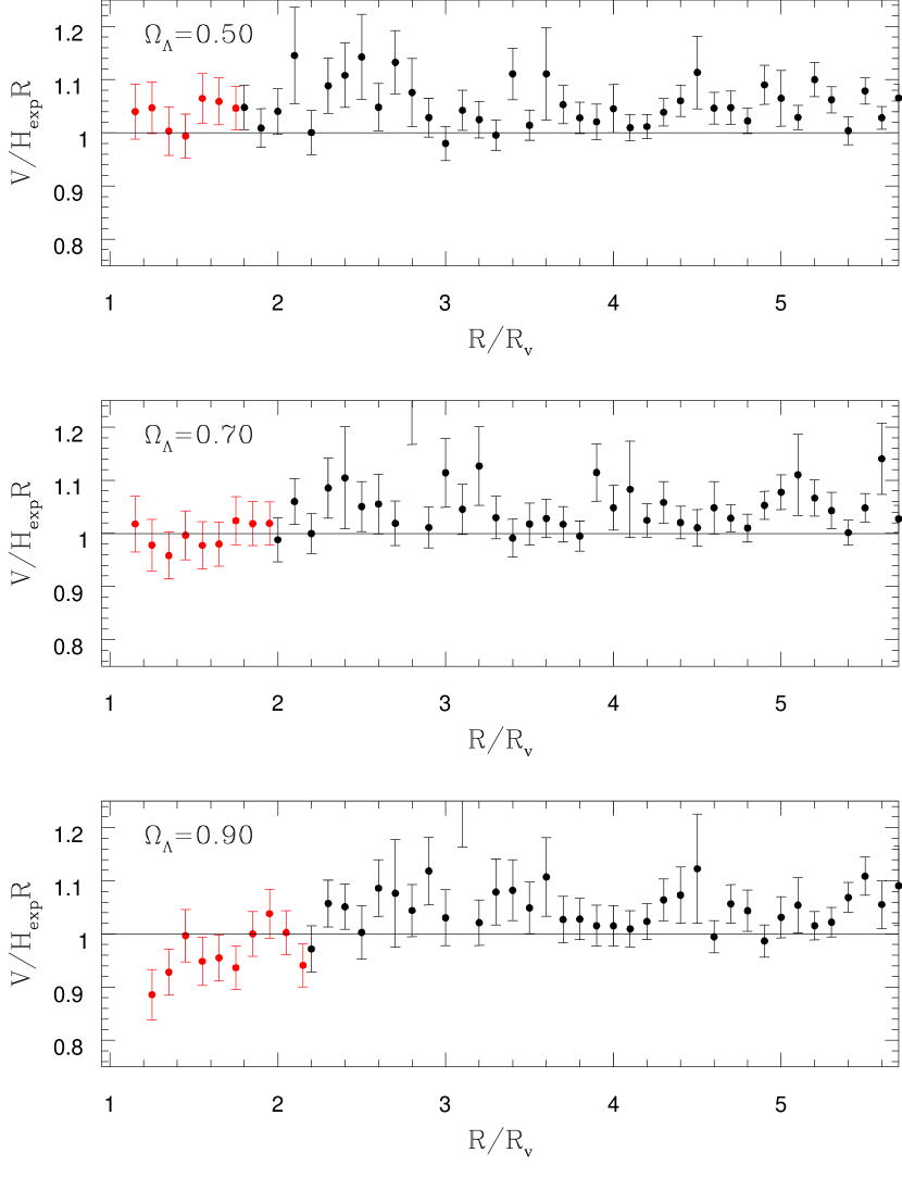
The main results of this work are summarized in Fig. 5 which shows how the solutions vary as a function $\Omega_{\Lambda}$ or degree of sub-Hubble expansion. The statistic in the individual panels in Fig. 5 was determined in exactly the same manner as that in the simulation in Fig. 2. Red points represent $Y(H_{v})$ and black points $Y(H(z_{g})$. To the left of the break at $R/R_{v}\sim 2$ these ordinates are plotted against $R(H_{v})/R_{v}$ while to the right against $R(H(z_{g})/R_{v}$. The same groups were used to construct each panel. These included those with $2.6<R_{v}(h^{-1}_{70}Mpc)<3.3$ in the middle panel. The large scatter, particularly among the black points, is generally to values greater than unity. The most deviant among these points also tend to show the largest uncertainties. As discussed earlier, the full effects of the peculiar motions are assumed to be causing this bias. The red points represent a region with a cooler flow so that this bias should be negligible here. Giving most weight to the red points, we adopt the value of $\Omega_{\Lambda}\sim 0.7$ and based on the spread of the mean of the red points from each panel assign an uncertainty of $\pm 0.1$. Using the more direct approach T08 find $\Omega_{\Lambda}\sim 0.77$ from known distances and velocities. Finally we note from Fig. 1 of T10 that the actual value of $H_{v}$ should increase slightly over the range $1<R(H_{v})/R_{v}<1.7$.

4 Summary and Conclusions

From a combination of geometry and statistics we have shown that the velocity field surrounding groups of galaxies obeys two Hubble like expansion laws i.e. $V=H_{exp}R$. At large distances the global Hubble Law is recovered. Within two well defined radii $R_{v}$ and $R_{ES}$ we find a lower expansion rate ($H_{exp}\sim 0.84H_{o}$). Thus the main result of this work is the demonstration that the phenomenon reported by T08 extends well beyond the vicinity of the local group. If one adopts the the interpretation of T08 that the result is due to the local effects of dark energy, we find $\Omega_{\Lambda}\sim(0.84)^{2}\sim 0.7\pm 0.1$ from a relatively small range of group mass. It is interesting that Sandage (1986), using the data then available, found that the calculated deceleration due to the Local Group is equivalent to $H_{exp}\sim 0.83H_{o}$ at a distance $\sim 1.6h^{-1}_{70}Mpc$ for an $\Omega_{0}=0$ $(\Lambda=0)$ cosmology.

These results do not contradict the conclusions from the cosmological simulations of Hoffman et al. (2008) & Martinez-Vaquero et al. (2009) that the ‘coolness’ of the local flow, by itself is not a strong discriminant between a model without $\Lambda$ (OCDM) and $\Lambda$CDM. Here the flow between $R_{v}$ and $R_{ES}$ is cooler because the galaxies within this region originated from inside the group and hence share the group’s peculiar motion. Galaxies beyond $R_{ES}$ feel the full effect of the peculiar motions. The observations show a systematic lowering of the expansion rate within the inner (cool flow) region in both of the OCDM and $\Lambda$CDM models. Based on the T08 interpretation the sub-Hubble rate in the $\Lambda$CDM model is predictable and when applied can account for the observations. However, interpreting the results as a local cosmological effect $does$ contradict the conclusions from the above simulations. Until this impasse is definitively resolved with further work one may consider $H_{v}$ to be a convenient parameterization of a sub-Hubble expansion rate.

In conclusion, significant perturbations to the global flow around galaxy groups beyond the Local Group are present. The sub-Hubble expansion rates are similar to those found recently by T08 around 3 nearby groups. The possibility that local dark energy effects are responsible makes the problem worthy of further investigation both observationally and theoretically.

5 Acknowledgements

The author acknowledges helpful discussions in the early stages of this work with Tony Burke and Chris Pritchet and financial support from an NSERC Canada Discovery grant. In addition the author thanks the referee for providing a very constructive report. He also gratefully acknowledges guest worker privileges at the Herzberg Institute of Astrophysics.

Figure 1: The geometry of the problem is shown. The group is at distance d_g while the field galaxy at $d_{f}$ subtends an angle $\alpha$ at the observer. See text for details.

Figure 2: The results of a simulation showing the average $V/H_{exp}R$ versus normalized distance from the group center $R/R_{v}$. In this simulation group properties were the same as used in the analysis of the observations of the field galaxies. Here the ‘field galaxies’ were assigned random angles of $\theta$, assigned random group-centric distances $R$ and given appropriate line of sight redshifts due either to global Hubble or sub-Hubble expansion about these centers if $R/R_{v}$ was greater than or less than 2. Three hundred field galaxies were randomly assigned to each of the 12620 groups. The result shown is for an ($\Omega_{m}=0.3,\Omega_{\Lambda}=0.7,\Omega_{k}=0$) cosmology. The red points then represent $Y(H_{exp})$ with $H_{exp}=H_{v}=0.84H_{o}$ while the black points show results with $H_{exp}=H(z_{g})$. Error bars here and in all of the following diagrams represent the standard error of the mean.

Figure 3: Average $V/H_{exp}R$ plotted against $R/R_{v}$ for the cosmology and the assumed expansion velocity indicated. Only groups with $2.6<R_{v}(h^{-1}_{70}Mpc)<3.3$ were included as it is within this interval that the break at $R/R_{v}\sim 2$ was most distinct. This point represents the transition from sub-Hubble to global Hubble expansion ($R_{ES}$). The bottom panel shows analogous results for an open cosmology. See the text for a discussion of the scatter in these plots. Note in the top panel how the $\Lambda$ model can account for the expansion velocities below the break.

Figure 4: Top and middle panels: Average $V/H_{exp}R$ plotted against $R_{v}$ for all 12577 groups with $R_{v}<5.7$ and for the two regions of $R/R_{v}$ indicated. As in the other figures red points represent $Y(H_{v})$ and black points $Y(H(z_{g}))$. The bottom panel is similar to the top but for a sub-sample of groups with no neighbor within $4h^{-1}_{70}Mpc$. If group clustering was influencing the results the largest difference would occur between $R_{v}$ of 1 and 2. The dotted lines indicate the region within which groups were used to construct Figs. 3 & 5.

Figure 5: The same as Fig.2 except now showing the results from an analysis of the group and field galaxy observations for three trial values of $\Omega_{\Lambda}$. As in the other figures red points represent $Y(H_{v})$ and black points $Y(H(z_{g}))$. Note that $R_{v}$ itself is dependent on the assumed value of $\Omega_{\Lambda}$.