Contents

Foreword

Michael Way & Catherine Naud 4

Introduction

Michael Way 5

On a new approach for estimating threshold crossing times
with an application to global warming

Victor H. de la Peña 8

Cosmology through the large-scale structure of the Universe

Eyal Kazin 13

On the Shoulders of Gauss, Bessel, and Poisson: Links,
Chunks, Spheres, and Conditional Models

William Heavlin 21

Mining Citizen Science Data: Machine Learning Challenges

Kirk Borne 24

Tracking Climate Models

Claire Monteleoni 28

Spectral Analysis Methods for Complex Source Mixtures

Kevin Knuth 31

Beyond Objects: Using Machines to Understand the Diffuse
Universe

J.E.G. Peek 35

Viewpoints: A high-performance high-dimensional exploratory
data analysis tool

Michael J. Way 44

Clustering Approach for Partitioning Directional Data in
Earth and Space Sciences

Christian Klose 46

Planetary Detection: The Kepler Mission

Jon Jenkins 52

Understanding the possible influence of the solar activity
on the terrestrial climate: a times series analysis approach

Elizabeth Martínez-Gómez 54

Optimal Scheduling of Exoplanet Observations Using Bayesian
Adaptive Exploration

Thomas J. Loredo 61

Beyond Photometric Redshifts using Bayesian Inference

Tamás Budavári 65

Long-Range Climate Forecasts Using Data Clustering and
Information Theory

Dimitris Giannakis 68

Comparison of Information-Theoretic Methods to estimate
the information flow in a dynamical system

Deniz Gencaga 72

Reconstructing the Galactic halo’s accretion history: A finite
mixture model approach

Duane Lee & Will Jessop 77

Program 78

Participants 79

Talk Video Links 82

Foreword

Michael Way
NASA/Goddard Institute for Space Studies
2880 Broadway
New York, New York, USA

Catherine Naud
Department of Applied Physics and Applied Mathematics
Columbia University, New York, New York, USA
and
NASA/Goddard Institute for Space Studies
2880 Broadway
New York, New York, USA

The purpose of the New York Workshop on Computer, Earth and Space Sciences is to bring together the New York area’s finest Astronomers, Statisticians, Computer Scientists, Space and Earth Scientists to explore potential synergies between their respective fields. The 2011 edition (CESS2011) was a great success, and we would like to thank all of the presenters and participants for attending.

This year was also special as it included authors from the upcoming book titled “Advances in Machine Learning and Data Mining for Astronomy.” Over two days, the latest advanced techniques used to analyze the vast amounts of information now available for the understanding of our universe and our planet were presented. These proceedings attempt to provide a small window into what the current state of research is in this vast interdisciplinary field and we’d like to thank the speakers who spent the time to contribute to this volume.

This year all of the presentations were video taped and those presentations have all been uploaded to YouTube for easy access. As well, the slides from all of the presentations are available and can be downloaded from the workshop website.

We would also like to thank the local NASA/GISS staff for their assistance in organizing the workshop; in particular Carl Codan and Patricia Formosa. Thanks also goes to Drs. Jim Hansen and Larry Travis for supporting the workshop and allowing us to host it at The Goddard Institute for Space Studies again.

Introduction

Michael Way
NASA/Goddard Institute for Space Studies
2880 Broadway
New York, New York, USA

This is the 2nd time I’ve co-hosted the New York Workshop on Computer, Earth, and Space Sciences (CESS). My reason for continuing to do so is that, like many at this workshop, I’m a strong advocate of interdisciplinary research. My own research institute (GISS) has traditionally contained people in the fields of Planetary Science, Astronomy, Earth Science, Mathematics and Physics. We believe this has been a recipe for success and hence we also continue partnerships with the Applied Mathematics and Statistics Departments at Columbia University and New York Unversity. Our goal with these on-going workshops is to find new partnerships between people/groups in the entire New York area who otherwise would never have the opportunity to meet and share ideas for solving problems of mutual interest.

My own science has greatly benefitted over the years via collaborations with people I would have never imagined working with 10 years ago. For example, we have managed to find new ways of using Gaussian Process Regression (a non-linear regression technique) (Way et al. 2009) by working with linear algebra specialists at the San Jose State University department of Mathematics and Computer Science. This has led to novel methods for inverting relatively large ($\sim$100,000$\times$100,000) non-sparse matrices for use with Gaussian Process Regression (Foster et al. 2009).

As we are all aware, many scientific fields are also dealing with a data deluge which is often approached by different disciplines in different ways. A recent issue of Science Magazine has discussed this in some detail (e.g. Baranuik 2011). It has also been discussed in the recent book “The Fourth Paradigm” Hey et al. (2009). What the Science articles made me the most aware of is my own continued narrow focus. For example, there is a great deal that could be shared between the people at this workshop and the fields of Biology, Bio-Chemistry, Genomics and Ecologists to name a few from the Science article. This is particularly embarrassing for myself since in 2004 I attended a two-day seminar in Silicon Valley that discussed several chapters in the book “The Elements of Statistical Learning” (Hastie, Tibshirani, & Friedman 2003). Over 90% of the audience were Bio-Chemists, while I was only one of two Astronomers.

Another area which I think we can all agree most fields can benefit from is better (and cheaper) methods for displaying and hence interrogating our data. Later today I will discuss a program called viewpoints (Gazis, Levit, & Way 2010) which can be used to look at modest sized multivariate data sets on an individual desktop/laptop. Another of the Science Magazine articles (Fox & Hendler 2011) discusses a number of ways to look at data in less expensive way.

In fact several of the speakers at the CESS workshop this year are also contributors to a book in progress (Way et al. 2011) that has chapters written by a number of people in the fields of Astronomy, Machine Learning and Data Mining who have themselves engaged in interdisciplinary research – this being one of the rationales for inviting them to contribute to this volume.

Finally, although I’ve restricted myself to the “hard sciences” we should not forget that interdisciplinary research is taking place in areas that perhaps only a few of us are familiar with. For example, I can highly recommend a recent book (Morris 2010) that discusses possible theories for the current western lead in technological innovation. The author (Ian Morris) uses data and methodologies from the fields of History, Sociology, Anthropology/Archaeology, Geology, Geography and Genetics to support the thesis in the short title of his book: “Why The West Rules – For Now”.

Regardless, I would like to thank all of the speakers for coming to New York and also for contributing to the workshop proceedings.

On a new approach for estimating threshold crossing times with an application to global warming

Victor J. de la Peña
Columbia University
Department of Statistics
New York, New York, USA

Abstract

Given a range of future projected climate trajectories taken from a multitude of models or scenarios, we attempt to find the best way to determine the threshold crossing time. In particular, we compare the proposed estimators to the more commonly used method of calculating the crossing time from the average of all trajectories (the mean path) and show that the former are superior in different situations. Moreover, using one of the former approaches also allows us to provide a measure of uncertainty as well as other properties of the crossing times distribution. In the cases with infinite first-hitting time, we also provide a new approach for estimating the cross time and show that our methods perform better than the common forecast. As a demonstration of our method, we look at the projected reduction in rainfall in two subtropical regions: the US Southwest and the Mediterranean.
 
KEY WORDS: Climate change; First-hitting time; Threshold-crossing; Probability bounds; Decoupling.

Introduction: Data and Methods

The data used to carry out the demonstration of the proposed method are time series of Southwest (U.S.) and Mediterranean region precipitation, calculated from IPCC Fourth Assessment (AR4) model simulations of the twentieth and twenty-first centuries (Randall et al. 2007). To demonstrate the application of our methods, simulated annual mean precipitation time series, area averaged over the US West ($125^{\circ}$W to $95^{\circ}$W and $25^{\circ}$N to $40^{\circ}$N) and the Mediterranean ($30^{\circ}$N to $45^{\circ}$N and $10^{\circ}$W to $50^{\circ}$E), were assembled from nineteen models. Refer to Seager et al. (2007) and the references therein for details.

Optimality of an unbiased estimator

An unbiased estimator

Before discussing the two possible estimators, we define $\boldsymbol{X}(t)=\{X_{1}(t),\ldots,X_{n}(t)\}$ be the outcomes of $n$ models (stochastic processes in the same probability space). The first hitting time of the $i$th simulated path $X_{i}$ with $T$ bounded is defined as

$$T_{r,i}:=\inf\left\{t\in[0,\tau]:X_{i}(t)\geq r\right\}\text{ where }X_{i}(t)\geq 0\leavevmode\nobreak\ \leavevmode\nobreak\ \leavevmode\nobreak\ \leavevmode\nobreak\ ,\leavevmode\nobreak\ \leavevmode\nobreak\ \leavevmode\nobreak\ i=1,\ldots,n(=19).$$

Unless otherwise known, we assume that the paths are equally likely to be close to the “true” path. Therefore, we let

$$T_{r}=T_{j}\text{ with probability }\frac{1}{n}\leavevmode\nobreak\ \leavevmode\nobreak\ \leavevmode\nobreak\ \leavevmode\nobreak\ ,\leavevmode\nobreak\ \leavevmode\nobreak\ \leavevmode\nobreak\ \leavevmode\nobreak\ j=1,\ldots,n(=19),$$ (1)

where $T_{r}$ denotes the true path. There are two possible ways to estimate the first-hitting time of the true path, namely

1. Mean of the first-hitting time:

   $$T^{(UF)}_{r}:=\frac{1}{n}\sum^{n}_{i=1}T_{r,i},$$

2. First-hitting time of the mean path:

   $$T^{(CF)}_{r}:=\inf\left\{t\in[0,\tau]:\bar{X}_{n}(t):=\frac{1}{n}\sum^{n}_{i=1}X_{i}(t)\geq r\right\}.$$

Proposition 0.1.

The unbiased estimator $T^{(UF)}_{b}$ outperforms the traditional estimator $T^{(CF)}_{b}$ in terms of (i) mean-squared error and (ii) Brier skill score. $a^{-1}_{(n)}(r)$, to be specified in Theorem 3.1, is preferred in cases where $T^{(UF)}_{r}=\infty$.
 
Remark: By considering the crossing times of individual paths, we can obtain an empirical CDF for $T_{r}$, which is useful for modeling various statistical properties of $T_{r}$.

Extending boundary crossing of non-random functions to that of stochastic processes

In the situations in which not all the simulated paths cross the boundary before the end of the experiment, we propose a remedy which can be summarized in the following theorem. For details, refer to Brown et al. (2011)

Theorem 0.1.

Let $X_{s}\geq 0$, $a_{(n)}(t)=E\sup_{s\leq t}X_{s}=n^{-1}\sum^{n}_{i=1}\sup_{s\leq t}Y_{s,i}$. Assume $a_{n}(t)$ is increasing (we can also use a generalized inverse) with $a_{(n)}^{-1}(r)=t_{r}=\inf\{t>0:a_{(n)}(t)=r\}\longrightarrow a(t)$, we can obtain bounds, under certain conditions:

$$\frac{1}{2}a_{(n)}^{-1}(r/2)\leq E[T_{r}]\leq 2a_{(n)}^{-1}(r),$$

Remark: The lower bound is universal.

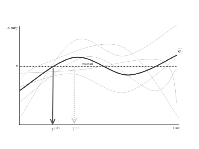
Figure 1: Illustrating how to obtain $T^{(UF)}$ and $T^{(CF)}$

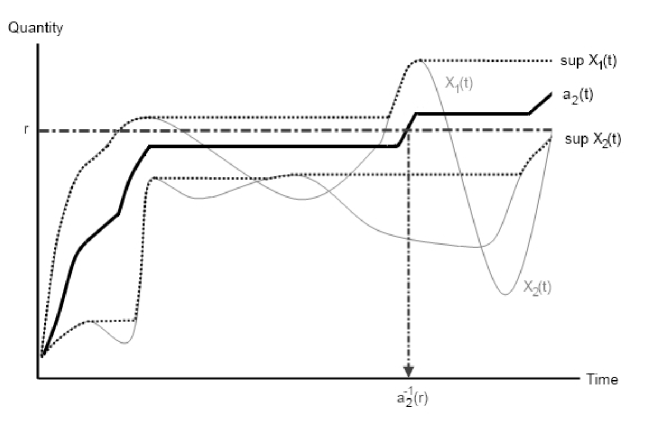
Figure 2: Illustration of $a_{(n)}(t)$ and $a_{(n)}^{-1}(r)$.

Results

Details of the results are tabulated as follows:

	$T^{(UF)}:=\sum n^{-1}T_{i}$	$T^{(CF)}(n^{-1})$	$\hat{M}$	$a^{-1}_{(n)}(r)$
Mediterranean	2010.21	2035	2018	2008
Southwest US	$\infty$	2018	2011	2004

where $T^{(UF)}$, $T^{(CF)}$, $\hat{M}$ and $a^{-1}_{(n)}(r)$ denote respectively the mean hitting times of the simulated paths, the hitting time of the mean simulated path, the median hitting times of the simulated paths and the hitting time estimate based on Theorem 3.1. 19 paths are simulated for both Mediterranean and Southwest US regions. The infinity value for the Southwest US region is due to the fact that there are three paths that do not cross the boundary. If we just include the paths that cross the boundary, we will have $T^{(UF)}=2004.63$. Clearly, in the case of Southwest,$a_{(}n)^{-1}(r)$ is better than $T_{r}$ wich has infinite expectation. 

According to the current estimates, the drought in the Southwest region is already in process. This observation shows a case where $T^{(UF)}$ and $a^{-1}_{(n)}(r)$ provide better forecasts than $T^{(CF)}$ or the median.

Cosmology through the large-scale structure of the Universe

Eyal A. Kazin
Center for Cosmology and Particle Physics
New York University, 4 Washington Place
New York, NY 10003, USA

Abstract

The distribution of matter contains a lot of cosmological information. Applying N-point statistics one can measure the geometry and expansion of the cosmos as well as test General Relativity at scales of millions to billions of light years. In particular, I will discuss an exciting recent measurement dubbed the “baryonic acoustic feature”, which has recently been detected in the Sloan Digital Sky Survey galaxy sample. It is the largest known “standard ruler” (half a billion light years across), and is being used to investigate the nature of the acceleration of the Universe.

The questions posed by $\Lambda$CDM

The Cosmic Microwave Background (CMB) shows us a picture of the early Universe which was very uniform (Penzias & Wilson 1965), yet with enough inhomogeneities (Smoot et al. 1992) to seed the structure we see today in the form of galaxies and the cosmic-web. Ongoing sky surveys are measuring deeper into the Universe with high edge technology transforming cosmology into a precision science.

The leading “Big Bang” model today is dubbed $\Lambda$CDM. While shown to be superbly consistent with many independent astronomical probes, it indicates that the “regular” material (atoms, radiation) comprise of only $5\%$ of the energy budget, hence challenging our current understanding of physics.

The $\Lambda$ is a reintroduction of Einstein’s so-called cosmological constant. He originally introduced it to stabilize a Universe that could expand or contract, according to General Relativity. At present, it is considered a mysterious energy with a repulsive force that explains the acceleration of the observed Universe. This acceleration was first noticed through super-novae distance-redshift relationships (Riess et al. 1998, Perlmutter et al. 1999). Often called dark energy, it has no clear explanation, and most cosmologists would happily do away with it, once a better intuitive explanation emerges. One stream of thought is modifying General Relativity on very large scales, e.g, by generalizing to higher dimensions.

Cold dark matter (CDM), on the other hand, has gained its “street-cred” throughout recent decades, as an invisible substance (meaning not interacting with radiation), but seen time and time again as the dominant gravitational source. Dark matter is required to explain various measurements as the virial motions of galaxies within clusters (Zwicky 1933), the rotation curves of galaxies (Rubin & Ford 1970), the gravitational lensing of background galaxies, and collisions of galaxy clusters (Clowe et al. 2004). We have yet to detect dark matter on Earth, although there already have been false positives. Physicists hope to see convincing evidence emerge from the Large Hadron Collider which is bashing protons at near the speed of light.

One of the most convincing pieces of evidence for dark matter is the growth of the large-scale structure of the Universe, the subject of this essay. The CMB gives us a picture of the Universe when it was one thousand time smaller than present. Early Universe inhomogeneities seen through temperature fluctuations in the CMB are of the order one part in $10^{5}$. By measuring the distribution of galaxies, the structure in the recent Universe is probed to percent level at scales of hundreds of millions of light-year scales and it can also be probed at the unity level and higher at “smaller” cosmic scales of thousands of light-years. These tantalizing differences in structure can not be explained by the gravitational attraction of regular material alone (atoms, molecules, stars, galaxies etc.), but can be explained with non-relativistic dark matter. Similar arguments show that the dark matter consists of $\sim 20\%$ of the energy budget, and dark energy $\sim 75\%$.

The distribution of matter, hence, is a vital test for any cosmological model.

Acoustic oscillations as a cosmic ruler

Recently an important feature dubbed the baryonic acoustic feature has been detected in galaxy clustering (Eisenstein et al. 2005, Percival et al. 2010, Kazin et al. 2010). The feature has been detected significantly in the anisotropies of the CMB by various Earth and space based missions (e.g. Torbet et al. 1999, Komatsu et al. 2009). Hence, cosmologists have made an important connection between the early and late Universe.

When the Universe was much smaller than today, energetic radiation dominated and did not enable the formation of atoms. Photon pressure on the free electrons and protons (collectively called baryons), caused them to propagate as a fluid in acoustic wave fashion. A useful analogy to have in mind is a pebble dropped in water perturbing it and forming a wave.

As the Universe expanded it cooled down and the first atoms formed freeing the radiation, which we now measure as the CMB. Imagine the pond freezing, including the wave. As the atoms are no longer being pushed they slow down, and are now gravitationally bound to dark matter.

This means that around every over density, where the plasma-photon waves (or pebble) originated, we expect an excess of material at a characteristic radius of the wave when it froze, dubbed the sound horizon.

In practice, this does not happen in a unique place, but throughout the whole Universe (think of throwing many pebbles into the pond). This means that we expect to measure a characteristic correlation length in the anisotropies of the CMB, as well as in the clustering of matter in a statistical manner. Figure 1 demonstrates the detection of the feature in the CMB temperature anisotropies (Larson et al. 2011) and in the clustering of luminous red galaxies (Eisenstein et al. 2001).

As mentioned before, the $\sim 10^{5}$ increase in the amplitude of the inhomogeneities between early (CMB) and late Universe (galaxies) is explained very well with dark matter. The height of the baryonic acoustic feature also serves as a firm prediction of the CDM paradigm. If there was no dark matter, the relative amplitude of the feature would be much higher. An interesting anecdote is that we happen to live in an era when the feature is still detectable in galaxy clustering. Billions of years from now, it will be washed away, due to gravitational interplay between dark matter and galaxies.

In a practical sense, as the feature spans a characteristic scale, it can be used as a cosmic ruler. The signature in the anisotropies of the CMB (Figure 1a), calibrates this ruler by measuring the sound-horizon currently to an accuracy of $\sim 1.5\%$ (Komatsu et al. 2009).

By measuring the feature in galaxy clustering transverse to the line-of-sight, you can think of it as the base of a triangle, for which we know the observed angle, and hence can infer the distance to the galaxy sample. Clustering along the line-of-sight is an even more powerful measurement, as it is sensitive to the expansion of the Universe. By measuring expansion rates one can test effects of dark energy. Current measurements show that the baryonic acoustic feature in Figure 1b, can be used to measure the distance to $\sim 3.5$ billion light-years to an accuracy of $\sim 4\%$ (Percival et al. 2010, Kazin et al. 2010).

Clustering- the technical details

As dark matter can not be seen directly, luminous objects, as galaxies, can serve as tracers, like the tips of icebergs. Galaxies are thought to form in regions of high dark matter density. An effective way to measure galaxy clustering (and hence inferring the matter distribution) is through two-point correlations of over-densities.

An over-density at point $\vec{x}$ is defined as the contrast to the mean density $\overline{\rho}$:

$$\delta(\vec{x})\equiv\frac{\rho(\vec{x})}{\overline{\rho}}-1.$$ (2)

The auto-correlation function, defined as the joint probability of measuring an excess of density at a given separation $r$ is defined as:

$$\xi(r)\equiv\langle{\delta(\vec{x})\delta(\vec{x}+\vec{r})}\rangle,$$ (3)

where the average is over the volume, and the cosmological principle assumes statistical isotropy. This is related to the Fourier complementary power spectrum P($k$).

For P$(k)$, it is common to smooth out the galaxies into density fields, Fourier transforming $\delta$ and convolving with a “window function” that describes the actual geometry of the survey.

The estimated $\xi$, in practice, is calculated by counting galaxy pairs:

$$\hat{\xi}(r)=\frac{DD(r)}{RR(r)}-1,$$ (4)

where $DD(r)$ is the normalized number of galaxy pairs within a spherical shells of radius $r\pm\frac{1}{2}\Delta r$. This is compared to random points distributed according to the survey geometry, where $RR$ is the random-random normalized pair count. By normalized I refer to the fact that one uses many more random points than data points to reduce Poisson shot noise. Landy & Szalay (1993) show that an estimator that minimizes the variance is:

$$\hat{\xi}(r)=\frac{DD(r)+RR(r)-2DR(r)}{RR(r)},$$ (5)

where $DR$ are the normalized data-random pairs.

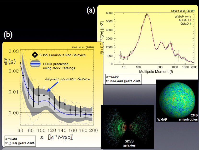
Figure 1: The baryonic acoustic feature in the large-scale structure of the Universe. The solid lines are $\Lambda$CDM predictions. (a) Temperature fluctuations in the CMB (2D projected $k$-space), measured by WMAP, ACBAR and QUaD. The feature is the form of peaks and troughs, and is detected to very high significance. These anisotropies are at the level of $10^{-5}$, and reflect the Universe as it was 1000-fold smaller than today ($\sim 13.3$ billion year ago). (b) SDSS luminous galaxy 3D clustering $\xi$ at very large scales ($100$ $h^{-1}$Mpc corresponds to $\sim 0.5$ billion light years). The feature is detected consistent with predictions. Notice $\xi$ is of order $1\%$ at the feature, showing a picture of the Universe $\sim 3$ billion years ago. The gray regions indicate $68,\ 95\%$ CL regions of simulated mock galaxy catalogs, reflecting cosmic variance. These will be substantially reduced in the future with larger volume surveys. (ABB means time “after big bang”)

The Sloan Digital Sky Survey

Using a dedicated $2.5$ meter telescope, the SDSS has industrialized (in a positive way!) astronomy. In January 2011, they publicly released an image of one third of the sky, and detected $469$ million objects from astroids to galaxies (SDSS-III collaboration: Hiroaki Aihara et al. 2011).

These images give a 2D projected image of the Universe. This is followed up by targeting objects of interest, obtaining their spectroscopy. The spectra contains information about the composition of the objects. As galaxies and quasars have signature spectra, these can be used as a templates to measure the Doppler-shift. The expanding Universe causes these to be redshifted. The redshift $z$ can be simply related to the distance $d$ through the Hubble equation at low $z$:

$$cz=Hd,$$ (6)

where $c$ is the speed of light and the Hubble parameter $H$ [1/time] is the expansion rate of the Universe. Hence, by measuring $z$, observers obtain a 3D picture of the Universe, which can be used to measure clustering. Dark energy effects Equation 6 through $H(z)$, when generalizing for larger distances.

The SDSS team has obtained spectroscopic redshifts of over a million objects in the largest volume to date. It is now in its third phase, obtaining more spectra for various missions including: improving measurements of the baryonic acoustic feature (and hence measuring dark energy) by measuring a larger and deeper volume, learning the structure of the Milky Way, and detection of exoplanets (Eisenstein et al. 2011).

Summary

Cosmologists are showing that there is much more than meets the eye. It is just a matter of time until dark matter will be understood, and might I be bold enough to say harnessed? The acceleration of the Universe, is still a profound mystery, but equipped with tools such as the baryonic acoustic feature, cosmologists will be able to provide rigorous tests.

E.K was partially supported by a Google Research Award and NASA Award NNX09AC85G.

On the Shoulders of Gauss, Bessel, and Poisson: Links, Chunks, Spheres, and Conditional Models

William D Heavlin
Google, Inc.
Mountain View, California, USA

Abstract

We consider generalized linear models (GLMs) and the associated exponential family (“links”). Our data structure partitions the data into mutually exclusively subsets (“chunks”). The conditional likelihood is defined as conditional on the within-chunk histogram of the response. These likelihoods have combinatorial complexity. To compute such likelihoods efficiently, we replace a sum over permutations with an integration over the orthogonal or rotation group (“spheres”). The resulting approximate likelihood gives rise to estimates that are highly linearized, therefore computationally attractive. Further, this approach refines our understanding of GLMs in several directions.

Notation and Model

Our observations are chunked into subsets indexed by $g:$ $(y_{gi},\mathbf{x}_{gi}:\;g=1,2,\ldots,G;\>i=1,\ldots,n_{g})$. The g-th chunk’s responses are denoted by $\mathbf{y}_{g}=(y_{g1},y_{g2},\ldots,y_{gn_{g}})$ and its feature matrix by $\mathbf{X}_{g};$ its i-th row is $\mathbf{x}_{gi}^{\mathbf{T}}.$ Our framework is that of the generalized linear model (McCullough & Nelder 1999):

$$\Pr\{y_{gi}|\mathbf{x}_{gi}^{\mathbf{T}}\mathbf{\beta}\}=\exp\{y_{gi}\mathbf{x}_{gi}^{\mathbf{T}}\mathbf{\beta})+h_{1}(y_{gi})+h_{2}(\mathbf{x}_{gi}^{\mathbf{T}}\mathbf{\beta})\}.$$ (7)

The Spherical Approximation

Motivated by the risk of attenuation, we condition ultimately on the variance of $\mathbf{y}_{g}.$ The resulting likelihood consists of these terms, indexed by $g:$

$$\exp\{L_{cg}(\mathbf{\beta})\}\approx\frac{\exp\{\mathbf{y}_{g}^{\mathbf{T}}\mathbf{X}_{g}\mathbf{\beta}\}}{\mbox{ave}\{\exp\{\mathbf{y}_{g}^{\mathbf{T}}\mathbf{P}_{\tau}^{\mathbf{T}}\mathbf{X}_{g}\mathbf{\beta}\}|\tau\in\mbox{orthogonal}\}}$$ (8)

Free of intercept terms, this likelihood resists attenuation. The rightmost term of (8) reduces to the von Mises-Fisher distribution (Mardia & Jupp 2000, Watson & Williams 1956) and is computationally attractive (Plis et al. 2010).

Figure 1 assesses the spherical approximation. The x-axis is the radius $\kappa=||\mathbf{y}_{g}||\times||\mathbf{X}_{g}\mathbf{\beta}||$, the y-axis the differential effect of equation (8)’s two denominators. Panel (c) illustrates how larger chunk sizes $n_{g}$ improve the spherical approximation. Panel (a) and (b) illustrates how the approximation for $n_{g}=2$ can be improved by a continuity correction.

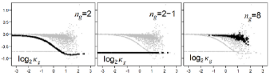
Figure 1: Numerically calculated values of $\frac{\partial}{\partial\kappa}\log Q$ as a function of radius $\kappa.$

Some Normal Equations

From (8) these maximum likelihood equations follow:

$$[\sum_{g}\frac{\rho_{g}}{r_{g}}\mathbf{X}_{g}^{\mathbf{T}}\mathbf{X}_{g}]\mathbf{\hat{\beta}}=\mathbf{X}_{g}^{\mathbf{T}}\mathbf{y}_{g},$$ (9)

which are nearly the same as those of Gauss. Added is the ratio $\rho_{g}/r_{g},$ which throttles chunks with less information; to first order, it equals the within-chunk variance.

The dependence of $\rho_{g}/r_{g}$ on $\mathbf{\beta}$ is weak, so the convergence of (9) is rapid. Equation (9) resembles iteratively reweighted least squares (Jorgensen 2006), but is more attractive computationally. To estimate many more features, we investigate marginal regression (Fan & Lv 2008) and boosting (Schapire & Singer 1999).

Conditional models like those in (8) do not furnish estimates of intercepts. The theory of conditional models therefore establishes a framework for multiple-stage modeling.

Mining Citizen Science Data: Machine Learning Challenges

Kirk Borne
School of Physics, Astronomy & Computational Science
George Mason University Fairfax, Virginia, USA

Large sky surveys in astronomy, with their open data policies (“data for all”) and their uniformly calibrated scientific databases, are key cyberinfrastructure for astronomical research. These sky survey databases are also a major content provider for educators and the general public. Depending on the audience, we recognize three broad modes of interaction with sky survey data (including the image archives and the science database catalogs). These modes of interaction span the progression from information-gathering to active engagement to discovery. They are:

• Data Discovery – What was observed, when, and by whom? Retrieve observation parameters from an sky survey catalog database. Retrieve parameters for interesting objects.

• Data Browse – Retrieve images from a sky survey image archive. View thumbnails. Select data format (JPEG, Google Sky KML, FITS). Pan the sky and examine catalog-provided tags (Google Sky, World Wide Telescope).

• Data Immersion – Perform data analysis, mining, and visualization. Report discoveries. Comment on observations. Contribute followup observations. Engage in social networking, annotation, and tagging. Provide classifications of complex images, data correlations, data clusters, or novel (outlying, anomalous) detections.

In the latter category are Citizen Science research experiences. The world of Citizen Science is blossoming in many ways, including century-old programs such as the Audubon Society bird counts and the American Association of Variable Star Observers (at aavso.org) continuous monitoring, measurement, collation, and dissemination of brightness variations of thousands of variable stars, but now including numerous projects in modern astronomy, climate science, biodiversity, watershed monitoring, space science, and more. The most famous and successful of these is the Galaxy Zoo project (at galaxyzoo.org), which is “staffed” by approximately 400,000 volunteer contributors. Modern Citizen Science experiences are naturally online, taking advantage of Web 2.0 technologies, for database-image-tagging mash-ups. It takes the form of crowd-sourcing the various stages of the scientific process. Citizen Scientists assist scientists’ research efforts by collecting, organizing, characterizing, annotating, and/or analyzing data. Citizen Science is one approach to engaging the public in authentic scientific research experiences with large astronomical sky survey databases and image archives.

Citizen Science is a term used for scientific research projects in which individual (non-scientist) volunteers (with little or no scientific training) perform or manage research-related tasks such as observation, measurement, or computation. In the Galaxy Zoo project, volunteers are asked to click on various pre-defined tags that describe the observable features in galaxy images – nearly one million such images from the SDSS (Sloan Digital Sky Survey, at sdss.org). Every one of these million galaxies has now been classified by Zoo volunteers approximately 200 times each. These tag data are a rich source of information about the galaxies, about human-computer interactions, about cognitive science, and about the Universe. The galaxy classifications are being used by astronomers to understand the dynamics, structure, and evolution of galaxies through cosmic time, and thereby used to understand the origin, state, and ultimate fate of our Universe. This illustrates some of the primary characteristics (and required features) of Citizen Science: that the experience must be engaging, must work with real scientific data, must not be busy-work, must address authentic science research questions that are beyond the capacity of science teams and computational processing pipelines, and must involve the scientists. The latter two points are demonstrated (and proven) by: (a) the sheer enormous number of galaxies to be classified is beyond the scope of the scientist teams, plus the complexity of the classification problem is beyond the capabilities of computational algorithms, primarily because the classification process is strongly based upon human recognition of complex patterns in the images, thereby requiring “eyes on the data”; and (b) approximately 20 peer- reviewed journal articles have already been produced from the Galaxy Zoo results – many of these papers contain Zoo volunteers as co-authors, and at least one of the papers includes no professional scientists as authors. The next major step in astronomical Citizen Science (but also including other scientific disciplines) is the Zooniverse project (at zooniverse.org). The Zooniverse is a framework for new Citizen Science projects, thereby enabling any science team to make use of the framework for their own projects with minimal effort and development activity. Currently active Zooniverse projects include Galaxy Zoo II, Galaxy Merger Zoo, the Milky Way Project, Supernova Search, Planet Hunters, Solar Storm Watch, Moon Zoo, and Old Weather. All of these depend on the power of human cognition (i.e., human computation), which is superb at finding patterns in data, at describing (characterizing) the data, and at finding anomalies (i.e., unusual features) in data. The most exciting example of this was the discovery of Hanny’s Voorwerp (Figure 1). A key component of the Zooniverse research program is the mining of the volunteer tags. These tag databases themselves represent a major source of data for knowledge discovery, pattern detection, and trend analysis. We are developing and applying machine learning algorithms to the scientific discovery process with these tag databases. Specifically, we are addressing the question: how do the volunteer-contributed tags, labels, and annotations correlate with the scientist-measured science parameters (generated by automated pipelines and stored in project databases)? The ultimate goal will be to train the automated data pipelines in future sky surveys with improved classification algorithms, for better identification of anomalies, and with fewer classification errors. These improvements will be based upon millions of training examples provided by the Citizen Scientists. These improvements will be absolutely essential for projects like the future LSST (Large Synoptic Survey Telescope, at lsst.org), since LSST will measure properties for at least 100 times more galaxies and 100 times more stars than SDSS. Also, LSST will do repeated imaging of the sky over its 10-year project duration, so that each of the roughly 50 billion objects observed by LSST will have approximately 1000 separate observations. These 50 trillion time series data points will provide an enormous opportunity for Citizen Scientists to explore time series (i.e., object light curves) to discover all types of rare phenomena, rare objects, rare classes, and new objects, classes, and sub-classes. The contributions of human participants may include: characterization of countless light curves; human-assisted search for best-fit models of rotating asteroids (including shapes, spin periods, and varying surface reflection properties); discovery of sub-patterns of variability in known variable stars; discovery of interesting objects in the environments around variable objects; discovery of associations among multiple variable and/or moving objects in a field; and more.

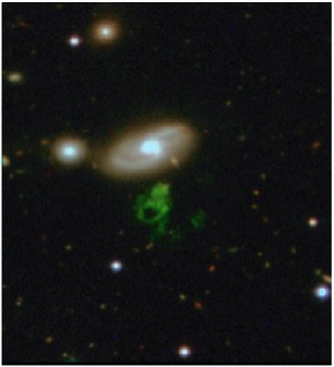
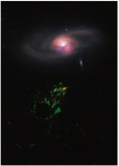
Figure 1: Hanny’s Voorwerp (Hanny’s Object) – The green gas cloud seen below the spiral galaxy in these images was first recognized as something unusual and “out of the ordinary” by Galaxy Zoo volunteer Hanny van Arkel, a Dutch school teacher, who was initially focused on classifying the dominant spiral galaxy above the green blob. This object is an illuminated gas cloud, glowing in the emission of ionized oxygen. It is probably the light echo from a dead quasar that was luminous at the center of the spiral galaxy about 100,000 years ago. These images are approximately true color. The left image was taken with a ground- based telescope, and the right image was obtained by the Hubble Space Telescope (courtesy W. Keel, the Galaxy Zoo team, NASA, and ESA).

As an example of machine learning the tag data, a preliminary study by (Baehr 2010) of the galaxy mergers found in the Galaxy Zoo I project was carried out. We found specific parameters in the SDSS science database that correlate best with “mergerness” versus “non-mergerness”. These database parameters are therefore useful in distinguishing normal (undisturbed) galaxies from abnormal (merging, colliding, interacting, disturbed) galaxies. Such results may consequently be applied to future sky surveys (e.g., LSST), to improve the automatic (machine-based) classification algorithms for colliding and merging galaxies. All of this was made possible by the fact that the galaxy classifications provided by Galaxy Zoo I participants led to the creation of the largest pure set of colliding and merging galaxies yet to be compiled for use by astronomers.

Tracking Climate Models

Claire Monteleoni
Center for Computational Learning Systems, Columbia University
New York, New York, USA

Gavin A. Schmidt
NASA Goddard Institute for Space Studies, 2880 Broadway
and
Center for Climate Systems Research, Columbia University
New York, New York, USA

Shailesh Saroha
Department of Computer Science
Columbia University
New York, New York, USA

Eva Asplund
Department of Computer Science, Columbia University
and
Barnard College
New York, New York, USA

Climate models are complex mathematical models designed by meteorologists, geophysicists, and climate scientists, and run as computer simulations, to predict climate. There is currently high variance among the predictions of 20 global climate models, from various laboratories around the world, that inform the Intergovernmental Panel on Climate Change (IPCC). Given temperature predictions from 20 IPCC global climate models, and over 100 years of historical temperature data, we track the changing sequence of which model currently predicts best. We use an algorithm due to Monteleoni & Jaakkola (2003), that models the sequence of observations using a hierarchical learner, based on a set of generalized Hidden Markov Models, where the identity of the current best climate model is the hidden variable. The transition probabilities between climate models are learned online, simultaneous to tracking the temperature predictions.

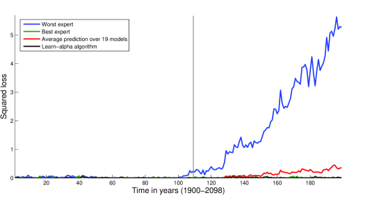
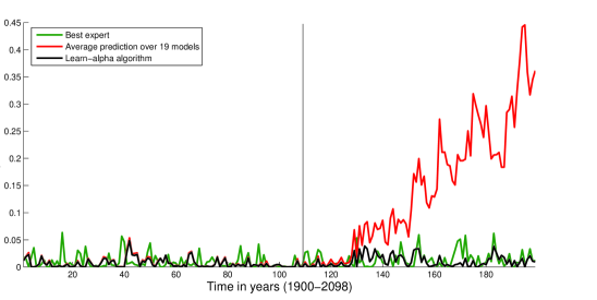
Figure 1: Global Future Simulation 1: Tracking the predictions of one model using the predictions of the remaining 19 as input, with no true temperature observations. Black vertical line separates past (hindcasts) from future predictions. Bottom plot zooms in on y-axis.

On historical global mean temperature data, our online learning algorithm’s average prediction loss nearly matches that of the best performing climate model in hindsight. Moreover its performance surpasses that of the average model prediction, which is the default practice in climate science, the median prediction, and least squares linear regression. We also experimented on climate model predictions through the year 2098. Simulating labels with the predictions of any one climate model, we found significantly improved performance using our online learning algorithm with respect to the other climate models, and techniques (see e.g. Figure 1). To complement our global results, we also ran experiments on IPCC global climate model temperature predictions for the specific geographic regions of Africa, Europe, and North America. On historical data, at both annual and monthly time-scales, and in future simulations, our algorithm typically outperformed both the best climate model per region, and linear regression. Notably, our algorithm consistently outperformed the average prediction over models, the current benchmark.

Spectral Analysis Methods for Complex Source Mixtures

Kevin H. Knuth
Departments of Physics and Informatics
University at Albany
Albany, New York, USA

Abstract

Spectral analysis in real problems must contend with the fact that there may be a large number of interesting sources some of which have known characteristics and others which have unknown characteristics. In addition, one must also contend with the presence of uninteresting or background sources, again with potentially known and unknown characteristics. In this talk I will discuss some of these challenges and describe some of the useful solutions we have developed, such as sampling methods to fit large numbers of sources and spline methods to fit unknown background signals.

Introduction

The infrared spectrum of star-forming regions is dominated by emission from a class of benzene-based molecules known as Polycyclic Aromatic Hydrocarbons (PAHs). The observed emission appears to arise from the combined emission of numerous PAH molecular species, both neutral and ionized, each with its unique spectrum. Unraveling these variations is crucial to a deeper understanding of star-forming regions in the universe. However, efforts to fit these data have been defeated by the complexity of the observed PAH spectra and the very large number of potential PAH emitters. Linear superposition of the various PAH species accompanied by additional sources identifies this problem as a source separation problem. It is, however, of a formidable class of source separation problems given that different PAH sources are potentially in the hundreds, even thousands, and there is only one measured spectral signal for a given astrophysical site. In collaboration with Duane Carbon (NASA Advanced Supercomputing Center, NASA Ames), we have focused on developing informed Bayesian source separation techniques (Knuth 2005) to identify and characterize the contribution of a large number of PAH species to infrared spectra recorded from the Infrared Space Observatory (ISO). To accomplish this we take advantage of a large database of over 500 atomic and molecular PAH spectra in various states of ionization that has been constructed by the NASA Ames PAH team (Allamandola, Bauschlicher, Cami and Peeters). To isolate the PAH spectra, much effort has gone into developing background estimation algorithms that model the spectral background so that it can be removed to reveal PAH, as well as atomic and ionic, emission lines.

The Spectrum Model

Blind techniques are not always useful in complex situations like these where much is known about the physics of the source signal generation and propagation. Higher-order models relying on physically-motivated parameterized functions are required, and by adopting such models, one can introduce more sophisticated likelihood and prior probabilities. We call this approach Informed Source Separation (Knuth et al. 2007). In this problem, we have linear mixing of P PAH spectra, K Planck blackbodies, a mixture of G Gaussians to describe unknown sources and additive noise:

$$F(\lambda)=\sum_{p=1}^{P}c_{p}PAH_{p}(\lambda)+\sum_{k=1}^{K}A_{k}Planck(\lambda;T_{k})+\sum_{g=1}^{G}A_{g}N(\lambda;\bar{\lambda_{g}},\sigma_{g})+\phi(\lambda)$$ (10)

where $PAH_{p}$ is a p-indexed PAH spectrum from the dictionary, $N$ is a Gaussian. The function Planck is

$$Planck(\lambda;T_{k})=\sqrt{\frac{\lambda_{max}}{\lambda}}\frac{exp(hc/\lambda_{max}kT)-1}{exp(hc/\lambda kT)-1}$$ (11)

where $h$ is Planck’s constant, $c$ is the speed of light, $k$ is Boltzmann’s constant, $T$ is the temperature of the cloud, and $\lambda_{max}$ is the wavelength where the blackbody spectral energy peaks $\lambda_{max}=hc/4.965kT$.

Source Separation using Sampling Methods

The sum over Planck blackbodies in the modeled spectrum (1) takes into account the fact that we are recording spectra from potentially several sources arranged along the line-of-sight. Applying this model in conjunction with a nested sampling algorithm to data recorded from ISO of the Orion Bar we were able to obtain reasonable background fits, which often showed the presence of multiple blackbodies. The results indicate that there is one blackbody radiator at a temperature of 61.043 $\pm$ 0.004 K, and possibly a second (36.3% chance), at a temperature around 18.8 K. Despite these successes, this algorithm did not provide adequate results for background removal since the estimated background was not constrained to lie below the recorded spectrum. Upon background subtraction, this led to unphysical negative spectral power. This result encouraged us to develop an alternative background estimation algorithm. Estimation of PAHs was demonstrated to be feasible in synthetic mixtures with low noise using sampling methods, such as Metropolis-Hastings Markov chain Monte Carlo (MCMC) and Nested Sampling. Estimation using gradient climbing techniques, such as the Nelder-Mead simplex method, too often were trapped in local solutions. In real data, PAH estimation was confounded by spectral background.

Background Removal Algorithm

Our most advanced background removal algorithm was developed to avoid the problem of negative spectral power by employing a spline-based model coupled with a likelihood function that favors background models that lie below the recorded spectrum. This is accomplished by using a likelihood function based on the Gaussian where the standard deviation on the negative side is 10 times smaller than on the positive side. The algorithm is designed with the option to include a second derivative smoothing prior. Users choose the number of spline knots and set their positions along the x-axis. This provides the option of fitting a spectral feature or estimating a smooth background underlying it. Our preliminary work shows that the background estimation algorithm works very well with both synthetic and real data (Nathan 2010). The use of this algorithm illustrates that PAH estimates are extremely sensitive to background, and that PAH characterization is extremely difficult in cases where the background spectra are poorly understood.

Kevin Knuth would like to acknowledge Duane Carbon, Joshua Choinsky, Deniz Gencaga, Haley Maunu, Brian Nathan and ManKit Tse for all of their hard work on this project.

Beyond Objects: Using Machines to Understand the Diffuse Universe

J. E. G. Peek
Department of Astronomy
Columbia University
New York, New York, USA

In this contribution I argue that our understanding of the universe has been shaped by an intrinsically “object-oriented” perspective, and that to better understand our diffuse universe we need to develop new ways of thinking and new algorithms to do this thinking for us.

Envisioning our universe in the context of objects is natural both observationally and physically. When our ancestors looked up into the the starry sky, they noticed something very different from the daytime sky. The nighttime sky has specific objects, and we gave them names: Rigel, Procyon, Fomalhaut, Saturn, Venus, Mars. These objects were both very distinct from the blackness of space, but they were also persistent night to night. The same could not be said of the daytime sky, with its amorphous, drifting clouds, never to be seen again, with no particular identity. Clouds could sometimes be distinguished from the background sky, but often were a complex, interacting blend. From this point forward astronomy has been a science of objects. And we have been rewarded for this assumption: stars in space can be thought of very well as discrete things. They have huge density contrasts compared to the rest of space, and they are incredibly rare and compact. They rarely contact each other, and are typically easy to distinguish. The same can be said (to a lesser extent) of planets and galaxies, as well as all manner of astronomical objects.

I argue, though, that we have gotten to a stage of understanding of our universe that we need to be able to better consider the diffuse universe. We now know that the material universe is largely made out of the very diffuse dark matter, which, while clumpy, is not well approximated as discrete objects. Even the baryonic matter is largely diffuse: of the 4% of the mass-energy budget of the universe devoted to baryons, 3.5% is diffuse hot gas permeating the universe, and collecting around groups of galaxies. Besides the simple accounting argument, it is important to realize that the interests of astronomers are now oriented more and more toward origins: origins of planets, origins of stars, origins of galaxies. This is manifest in the fact that NASA devotes a plurality of its astrophysics budget to the “cosmic origins” program. And what do we mean by origins? The entire history of anything in the universe can be roughly summed up as “it started diffuse and then, under the force of gravity, it became more dense”. If we are serious about understanding the origins of things in the universe, we must do better at understanding not just the objects, but the diffuse material whence they came.

We have, as investigators of the universe, enlisted machines to do a lot of our understanding for us. And, as machines inherit our intuition through the codes and algorithms we write, we have given them a keen sense of objects. A modern and powerful example is the Sloan Digital Sky Survey (SDSS; York et al. 2000). SDSS makes huge maps of the sky with very high fidelity, but these maps are rarely used for anything beyond wall decor. The real power of the SDSS experiment depends on the photometric pipeline (Lupton et al. 2001), which interprets that sky into tens of millions of objects, each with precise photometric information. With these lists in hand we can better take a census of the stars and galaxies in our universe. It is sometimes interesting to understand the limits of these methodologies; the photo pipeline can find distant galaxies easily, but large, nearby galaxies are a challenge, as the photo pipeline cannot easily interpret these huge diaphanous shapes (West et al. 2010; Fig 1). The Virtual Astronomical Observatory (VAO; e.g. Hanisch 2010) is another example of a collection of algorithms that enables our object-oriented mindset. VAO has developed a huge set of tools that allow astronomers to collect a vast array of information from different sources, and combine them elegantly together. These tools, however, almost always use the “object” as the smallest element of information, and are much less useful in interpreting the diffuse universe. Finally, astrometry.net is an example of how cutting edge algorithms combined with excellent data can yield new tools for interpreting astronomical data (Lang et al. 2010). By accessing giant catalogs of objects, the software can, in seconds, give precise astrometric information about any image containing stars. Again, we leverage our object-oriented understanding, both both psychologically and computationally, to decode our data.

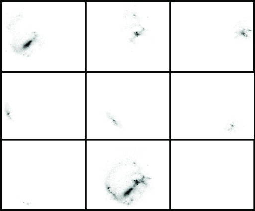
Figure 1: r-band atlas images for HIPEQ1124+03. A single galaxy has been divided into 7 sub-images by the SDSS photometric pipeline, which considered them individual objects. The original galaxy is shown in the lower-middle panel. Reprinted with permission from West et al. (2010).

As a case study, we examine at a truly object-less data space: the Galactic neutral hydrogen (H i) interstellar medium (ISM). Through the 21-cm hyperfine transition of H i, we can study the neutral ISM of our Galaxy and others both angularly and in the velocity domain (e.g. Kulkarni & Heiles 1988). H i images of other galaxies, while sometimes diffuse, do typically have clear edges. In our own Galaxy we are afforded no such luxury. The Galactic H i ISM is sky-filling, and can represent gas on a huge range of distances and physical conditions. As our technology increases, we are able to build larger and larger, and more and more detailed images of the H i ISM. What we see in these multi-spectral images is an incredible cacophony of shapes and structures, overlapping, intermingling, with a variety of size, shape, and intensity that cannot be easily described. Indeed, it is this lack of language that is at the crux of the problem. These data are affected by a huge number of processes; the accretion of material onto the Galaxy (e.g. Begum et al. 2010), the impact of shockwaves and explosions (e.g. Heiles 1979), the formation of stars (e.g. Kim et al. 1998), the effect of magnetization (e.g. McClure-Griffiths et al. 2006). And yet, we have very few tools that capture this information.

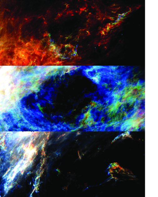
Figure 2: A typical region of the Galactic H i sky, 40${}^{\circ}\times 18^{\circ}$ $10^{\prime}$ in size. The top panel represents, -41.6, -39.4, -37.2  km s^-1 in red, green, and blue, respectively. The middle panel represents -4.0, -1.8, and 0.4 km ${\rm s^{-1}}$, while the bottom panel represents 15.8, 18.7, 21.7 km ${\rm s^{-1}}$. Reprinted with permission from (Peek et al. 2011).

As yet, there are two “flavors” of mechanisms we as a community have used to try to interpret this kind of diffuse data. The first is the observer’s method. In the observer’s method the data cubes are inspected by eye, and visually interesting shapes have been picked out (e.g. Ford et al. 2010). These shapes are then cataloged and described, usually qualitatively and without statistical rigor. The problems with these methods are self-evident: impossible statistics, unquantifiable biases, and an inability to compare to physical models. The second method is the theorist’s method. In the theorist’s method, some equation is applied to the data set wholesale, and a number comes out (e.g. Chepurnov et al. 2010). This method is powerful in that it can be compared directly to simulation, but typically cannot interpret any shape information at all. Given that the ISM is not a homogeneous, isotropic system, and various physical effects may influence the gas in different directions or at different velocities, this method seems a poor match for the data. It also cuts out any intuition as to what data may be carrying the most interesting information.

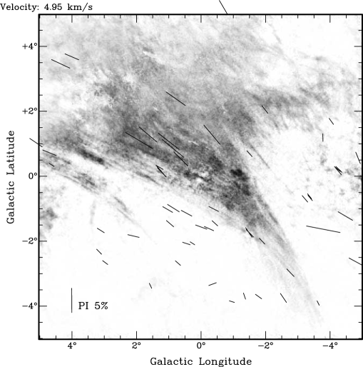
Figure 3: An H i image of the Riegel-Crutcher cloud from McClure-Griffiths et al. (2006) at 4.95  km s^-1 $v_{\rm LSR}$. The polarization vectors from background starlight indicate that the structure of the ISM reflects the structure of the intrinsic magnetization. Reprinted with permission from McClure-Griffiths et al. (2006).

We are in the process of developing a “third way”, which I will explain in two examples. Of the two projects, our more completed one is a search for compact, low-velocity clouds in the Galaxy (e.g. Saul et al. 2011). These clouds are inherently interesting as they likely probe the surface of the Galaxy as it interacts with the Galactic halo, a very active area of astronomical research. To do this our group, led by Destry Saul, wrote a wavelet-style code to search through the data cubes for isolated clouds that matched our search criteria. These clouds once found could then be “objectified”, quantified and studied as a population. In some sense, through this objectification, we are trying to shoehorn an intrinsically diffuse problem into the object-oriented style thinking we are trying to escape. This gives us the advantage that we can use well known tools for analysis (e.g. scatter plots), but we give up a perhaps deeper understanding of these structures from considering them in their context. The harder, and far less developed, project is to try to understand the meaning of very straight and narrow diffuse structures in the HI ISM at very low velocity. The HI ISM is suffused with “blobby filaments”, but these particular structures seem to stand out, looking like a handful of dry fettuccine dropped on the kitchen floor. We know that these kinds of structures can give us insight into the physics of the ISM: in denser environments it has been shown that more discrete versions of these features are qualitatively correlated with dust polarizations and the magnetic underpinning of the ISM (McClure-Griffiths et al. 2006). We would like to investigate these features more quantitatively, but we have not developed mechanisms to answer even the simplest questions. In a given direction how much of this feature is there? In which way is it pointing? What are its qualities? Does there exist a continuum of these features, or are they truly discrete? The “object-oriented” astronomer mindset is not equipped to address these sophisticated questions.

We are just beginning to investigate machine vision techniques for understanding these unexplored data spaces. Machine vision technologies are being developed to better parse our very confusing visual world using computers, such as in the context of object identification and the 3D reconstruction of 2D images (Sonka et al. 2008). Up until now, most astronomical machine vision problems have been embarrassingly easy; points in space are relatively simple to parse for machines. Perhaps the diffuse universe will be a new challenge for computer vision specialists and be a focal point for communication between the two fields. Machine learning methods, and human-aided data interpretation on large scales may also prove crucial to cracking these complex problems. How exactly we employ these new technologies in parsing our diffuse universe is very much up to us.

Viewpoints: A high-performance high-dimensional exploratory data analysis tool

Michael Way
NASA/Goddard Institute for Space Studies
2880 Broadway
New York, New York, USA

Creon Levit & Paul Gazis
NASA/Ames Research Center
Moffett Field, California, USA

Viewpoints (Gazis et al. 2010) is a high-performance visualization and analysis tool for large, complex, multidimensional data sets. It allows interactive exploration of data in 100 or more dimensions with sample counts, or the number of points, exceeding $10^{6}$ (up to $10^{8}$ depending on available RAM). Viewpoints was originally created for use with the extremely large data sets produced by current and future NASA space science missions, but it has been used for a wide variety of diverse applications ranging from aeronautical engineering, quantum chemistry, and computational fluid dynamics to virology, computational finance, and aviation safety. One of it’s main features is the ability to look at the correlation of variables in multivariate data streams (see Figure 1).

Viewpoints can be considered a kind of “mini” version of the NASA Ames Hyperwall (Sandstrom et al. 2003) which has been used for examining multi-variate data of much larger sizes (see Figure 2). Viewpoints has been used extensively as a pre-processor to the Hyperwall in that one can look at sub-selections of the full dataset (if the full data set cannot be run) prior to viewing it with the Hyperwall (which is a highly leveraged resource). Currently viewpoints runs on Mac OS, Windows and Linux platforms, and only requires a moderately new (less than 6 years old) graphics card supporting OpenGL.

More information can be found here:
http://astrophysics.arc.nasa.gov/viewpoints
You can download the software from here:
http://www.assembla.com/wiki/show/viewpoints/downloads

Figure 1: Viewpoints as a collaboration tool: Here one workstation with multiple screens is looking at the same multi-variate data on a laptop. Screen layout and setup can be saved to an xml file which allows one to retrace previous investigations.

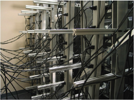
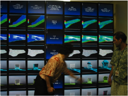
Figure 2: Left: The back of the original (7$\times$7 display) hyperwall at NASA/Ames. Right: The front of the hyperwall. One can see the obvious similarities between the Hyperwall and viewpoints.

Clustering Approach for Partitioning Directional Data in Earth and Space Sciences

C. D. Klose
Think GeoHazards
New York, New York, USA

K. Obermayer
Electrical Engineering and Computer Science
Technical University of Berlin
Berlin, Germany

Abstract

A simple clustering approach, based on vector quantization (VQ) is presented for partitioning directional data in Earth and Space Sciences. Directional data are grouped into a certain number of disjoint isotropic clusters, and at the same time the average direction is calculated for each group. The algorithm is fast, and thus can be easily utilized for large data sets. It shows good clustering results compared to other benchmark counting methods for directional data. No heuristics is being used, because the grouping of data points, the binary assignment of new data points to clusters, and the calculation of the average cluster values are based on the same cost function.

Keywords: clustering, directional data, discontinuities, fracture grouping

Introduction

Clustering problems of directional data are fundamental problems in earth and space sciences. Several methods have been proposed to help to find groups within directional data. Here, we give short overview on existing clustering methods of directional data and outline a new clustering method which is based on vector quantization (Gray 1984). The new method improves on several issues of clustering directional data and is published by Klose (2004).

Counting methods for visually partitioning the orientation data in stereographic plots were introduced by Schmidt (1925). Shanley & Mahtab (1976) and Wallbrecher (1978) developed counting techniques to identify clusters of orientation data. The parameters of Shanley & Mahtab’s counting method have to be optimized by minimizing an objective function. Wallbrecher’s method is optimized by comparing the clustering result with a given probability distribution on the sphere in order to obtain good partitioning results. However, counting methods depend on the density of data points and their results are prone to sampling bias (e.g., 1-D or 2-D sampling to describe a 3-D space). Counting methods are time-consuming, can lead to incorrect results for clusters with small dip angles, and can lead to solutions which an expert would rate sub-optimal. Pecher (1989) developed a supervised method for grouping of directional data distributions. A contour density plot is calculated and an observer picks initial values for the average dip directions and dip angles of one to a maximum of seven clusters. The method has a conceptual disadvantage. It uses two different distance measures; one measure for the assignment of data points to clusters and another measure defined by the orientation matrix to calculate the refined values for dip direction and dip angle. Thus, average values and cluster assignments are not determined in a self-consistent way.

Dershowitz et al. (1996) developed a partitioning method that is based on an iterative, stochastic reassignment of orientation vectors to clusters. Probability assignments are calculated using selected probability distributions on the sphere, which are centered on the average orientation vector that characterizes the cluster. The average orientation vector is then re-estimated using principal component analysis (PCA) of the orientation matrices. Probability distributions on the sphere were developed by several authors and are summarized in Fisher et al. (1987).

Hammah & Curran (1998) described a related approach based on fuzzy sets and on a similarity measure $d^{2}(\vec{x},\vec{w})=1-(\vec{x}^{T}\vec{w})^{2}$, where $\vec{x}$ is the orientation vector of a data point and $\vec{w}$ is the average orientation vector of the cluster. This measure is normally used for the analysis of orientation data (Anderberg 1973, Fisher et al. 1987).

Directional Data

Dip direction $\alpha$ and the dip angle $\theta$ of linear or planar structures are measured in degrees (^∘), where $0^{\circ}\leq\alpha\leq 360^{\circ}$ and $0^{\circ}\leq\theta\leq 90^{\circ}$. By convention, linear structures and normal vectors of planar structures, pole vectors $\vec{\Theta}=(\alpha,\theta)^{T}$, point towards the lower hemisphere of the unit sphere (Figure 1). The orientation $\vec{\Theta}^{A}=(\alpha^{A},\theta^{A})^{T}$ of a pole vector $A$ can be described by Cartesian coordinates $\vec{x}^{A}=(x_{1},x_{2},x_{3})^{T}$ (Figure 1), where

$$\begin{split}&x_{1}\;=\;cos(\alpha)\,cos(\theta)\hskip 28.45274pt\text{North direction}\\ &x_{2}\;=\;sin(\alpha)\,cos(\theta)\hskip 28.45274pt\text{East direction}\\ &x_{3}\;=\;sin(\theta)\hskip 65.44142pt\text{downward}.\end{split}$$ (12)

The projection $A^{\prime}$ of the endpoint $A$ of all given pole vectors onto the $x_{1}$-$x_{2}$ plane is called a stereographic plot (Figure 1) and is commonly used for visualisation purposes.

A) B)

Figure 1: A) Construction of a stereographic plot.
B) Stereographic plot with kernel density distribution.

The Clustering Method

Given are a set of $N$ pole vectors $\vec{x}_{k}$, $k=1,\ldots,N,$ (eq. 12). The vectors correspond to $N$ noisy measurements taken from $M$ orientation discontinuities whose spatial orientations are described by their (yet unknown) average pole vectors $\vec{w}_{l}$, $l=1,\ldots,M$. For every partition $l$ of the orientation data, there exists one average pole vector $\vec{w}_{l}$. The dissimilarity between a data point $\vec{x}_{k}$ and an average pole vector $\vec{w}_{l}$ is denoted by $d(\vec{x}_{k},\vec{w}_{l})$.

We now describe the assignment of pole vectors $\vec{x}_{k}$ to a partition by the binary assignment variables

$$m_{lk}\;=\;\left\{\begin{array}[]{ll}1,&\textrm{if data point $k$ belongs to cluster $l$}\\ 0,&\textrm{otherwise.}\end{array}\right.$$ (13)

One data point $\vec{x}_{k}$ belongs to only one orientation discontinuity $\vec{w}_{l}$. Here, the arc-length between the pole vectors on the unit sphere is proposed as the distance measure, i.e.

$$d(\vec{x},\vec{w})\;=\;\arccos\,(\,|\,\vec{x}^{T}\vec{w}\,|\,),$$ (14)

where $|.|$ denotes the absolute value.

The average dissimilarity between the data points and the pole vectors of the directional data they belong to is given by

$$E\;=\;\frac{1}{N}\sum_{k=1}^{N}\sum_{l=1}^{M}m_{lk}\,d(\vec{x}_{k},\vec{w}_{l}),$$ (15)

from which we calculate the optimal partition by minimizing the cost function $E$, i.e.

$$E\;\stackrel{{\scriptstyle!}}{{=}}\;\min_{\{m_{lk}\},\{\vec{w}_{l}\}}.$$ (16)

Minimization is performed iteratively in two steps. In the first step, the cost function $E$ is minimized with respect to the assignment variables $\{m_{lk}\}$ using

$$m_{lk}\;=\;\left\{\begin{array}[]{ll}1,&\mbox{\rm if}\;\;\;l\,=\,\arg\min_{q}\,d(\vec{x}_{k},\vec{w}_{q})\\ 0,&\mbox{\rm else.}\end{array}\right.$$ (17)

In the second step, cost $E$ is minimized with respect to the angles $\vec{\Theta_{l}}=(\alpha_{l},\theta_{l})^{T}$ which describe the average pole vectors $\vec{w}_{l}$ (see eq. (12)). This is done by evaluating the expression

$$\frac{\partial E}{\partial\vec{\Theta}_{l}}\;=\;\vec{0},$$ (18)

where $\vec{0}$ is a zero vector with respect to $\vec{\Theta}_{1}=(\alpha_{l},\theta_{l})^{T}$. This iterative procedure is called batch learning and converges to a minimum of the cost, because $E$ can never increase and is bounded from below. In most cases, however, a stochastic learning procedure called on-line learning is used which is more robust:

BEGIN Loop

Select a data point $\vec{x}_{k}$.

Assign data point $\vec{x}_{k}$ to cluster $l$ by:

$$l\;=\;\arg\min_{q}d(\vec{x}_{k},\vec{w}_{q})$$ (19)

Change the average pole vector of this cluster by:

$$\Delta\vec{\Theta}_{l}\;=\;-\gamma\frac{\partial d(\vec{x}_{k},\vec{w}_{l}(\vec{\Theta}_{l}))}{\partial\vec{\Theta}_{l}}$$ (20)

END Loop

The learning rate $\gamma$ should decrease with iteration number $t$, such that the conditions (Robbins & Monro 1951, Fukunaga 1990)

$$\sum_{t=1}^{\infty}\gamma(t)\;=\,\infty,\quad\textrm{and}\quad\sum_{t=1}^{\infty}\gamma^{2}(t)\;<\;\infty$$ (21)

are fulfilled.

Results

The clustering algorithm using the arc-length as distance measure is derived and applied in Klose et al.  (2004) and online available as a Java app (http://www.cdklose.com). First, the new clustering algorithm is applied to an artificial data set where orientation and distribution of pole vectors are statistically defined in advance. Second, the algorithm is applied to a real-world example given by Shanley & Mahtab (1976) (see Figure 1). Results are compared to existing counting and clustering methods, as described above.

Input	Output

Figure 2: Snapshots of the Java app of clustering algorithm available at http://www.cdklose.com

Planetary Detection: The Kepler Mission

Jon Jenkins
NASA/Ames Research Center
Moffett Field, California, USA

The Kepler telescope was launched into orbit in March 2009 to determine the frequency of Earth-sized planets transiting their Sun-like host stars in the habitable zone – that range of orbital distances for which liquid water would pool on the surface of a terrestrial planet such as Earth or Mars. This daunting task demands an instrument capable of measuring the light output from each of over 150,000 stars over a 115 square degree field of view simultaneously at an unprecedented photometric precision of 20 parts per million (ppm) on 6.5-hour intervals. Kepler is opening up a new vista in astronomy and astrophysics and is operating in a new regime where the instrumental signatures compete with the miniscule signatures of terrestrial planets transiting their host stars. The dynamic range of the intrinsic stellar variability observed in the light curves is breathtaking: RR Lyrae stars explosively oscillate with periods of approximately 0.5 days, doubling their brightness over a few hours. Some flare stars double their brightness on much shorter time scales at unpredictable intervals. At the same time, some stars exhibit quasi-coherent oscillations with amplitudes of 50 ppm that can be seen by eye in the raw flux time series. The richness of Kepler’s data lies in the huge dynamic range for the variations in intensity $>$10⁴ and the large dynamic range of time scales probed by the data, from a few minutes to weeks, months, and ultimately, to years.

Kepler is an audacious mission that places rigorous demands on the science pipeline used to process the ever-accumulating, large amount of data and to identify and characterize the minute planetary signatures hiding in the data haystack. We give an overview of the Science pipeline that reduces the pixel data to obtain flux time series and detect and characterize planetary transit signatures. In particular, we detail the adaptive, wavelet-based transit detector that performs the automated search through each light curve for transit signatures of Earth-sized planets. We describe a Bayesian Maximum A Posteriori (MAP) estimation approach under development to improve our ability to identify and remove instrumental signatures from the light curves that minimizes any distortion of astrophysical signals in the data and prevents the introduction of additional noise that may mask small, transit features, as indicated in the Figure 1. This approach leverages the availability of thousands of stellar targets on each CCD detector in order to construct an implicit forward model for the systematic error terms identified in the data as a whole. The Kepler Mission will not be the last spaceborne astrophysics mission to scan the heavens for planetary abodes. Several transit survey missions have been proposed to NASA and to ESA and some are under development. Clearly, these future missions can benefit from the lessons learned by Kepler and will face many of the same challenges that in some cases will be more difficult to solve given the significantly larger volume of data to be collected on a far greater number of stars than Kepler has had to deal with. Given the intense interest in exoplanets by the public and by the astronomical community, the future for exoplanet science appears to just be dawning with the initial success of the Kepler Mission.

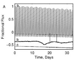
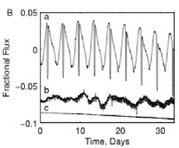
Figure 1: The light curves (a) for two stars on channel 2.1, along with (b) an LS fit to instrumental components extracted from the light curves and (c) a Bayesian Maximum A Posteriori (MAP) fit to the same instrumental components. Curves (b) and (c) have been offset from 0 for clarity. Panel A shows the results for an RR Lyrae star while panel B shows them for an eclipsing binary. Both light curves are dominated by intrinsic stellar variability rather than by instrumental signatures. The RR Lyrae doubles its brightness every 0.5 days, while the eclipsing binary exhibits spot variations that change slowly over time. The MAP fits do not corrupt the data with short term variations in the poorly matched instrumental signatures used in the fit, unlike the least squares fit.

Understanding the possible influence of the solar activity on the terrestrial climate: a times series analysis approach

Elizabeth Martínez-Gómez
Center for Astrostatistics
326 Thomas Building
The Pennsylvania State University
University Park, PA, USA

Víctor M. Guerrero
Departmento de Estadística
Instituto Tecnológico Autónomo de México
01080, Álvaro Obregón, México

Francisco Estrada
Centro de Ciencias de la Atmósfera
Universidad Nacional Autónoma de México
Ciudad Universitaria, 04510, Coyoacán, México

Abstract

Until the beginning of the 1980s, the relation between the Sun and climate change was still viewed with suspicion by the wider climate community and often remained a “taboo” subject in the solar astrophysics community. The main reason for this fact was a lack of knowledge about the causal link between the solar activity and its irradiance, that is, the amount of energy received at the average distance between the Earth and the Sun. For many years, some authors doubted about the invariability of the solar radiative output due to the apparent, but poorly explained, correlations between fluctuations of solar activity and atmospheric phenomena. Research on the mechanisms of solar effects on climate and their magnitude is currently benefiting from tremendous renewal of interest. A large amount of high resolution data is now available; however, the matter remains controversial because most of these records are influenced by other factors in addition to solar activity. In many works, the association between solar and terrestrial environmental parameters is found through some type of correlation based on multivariate statistics or applying the wavelet analysis on the corresponding time series data. The talk is divided in three parts. In the first I will review the solar- terrestrial climate problem. Later, I will focus on the time series analysis used in our study and finally, I will summarize our preliminary findings and comment further ideas to improve our model.

Review of the solar terrestrial problem

It is well-known that the Sun has an effect on terrestrial climate since its electromagnetic radiation is the main energy for the outer envelopes of Earth. This is one of the so called solar-terrestrial physics problems. This problem has been the subject of speculation and research by scientists for many years. Understanding the behavior of natural fluctuations in the climate is especially important because of the possibility of man-induced climate changes (Dingel & Landberg 1971, Schneider 1979, Tett et al. 1999). Many studies have been conducted to show correlations between the solar activity and various meteorological parameters but historical observations of solar activity were restricted to sunspot numbers and it was not clear how these could be physically related to meteorological factors. In this section we briefly describe some of the most remarkable characteristics of the solar activity and the terrestrial climate, emphasizing their possible connection.

a) Solar Activity

The term solar activity comprises photospheric and chromospheric phenomena such as sunspots, prominences and coronal disturbances. It has been measured via satellites during recent decades (for the Total Solar Irradiance, TSI) and through other “proxy” variables in prior times (for example, the daily observed number of sunspots, and the concentration of some cosmogenic isotopes in ice cores as ¹⁴C and ¹⁰Be).

The phenomena mentioned above are related to the variations of the solar magnetic field and the amount of received energy. Those are cyclic variations like the 11-year (sunspots), and 22-year (magnetic field reversion), among others.

b) Terrestrial climate

The Intergovernmental Panel on Climate Change (IPCC) glossary defines the climate as the “average weather,” or more rigorously, as the statistical description in terms of the mean and variability of relevant quantities (for example, temperature, precipitation, and wind) over a period of time ranging from months to thousands or millions of years.

c) Is there a connection between solar activity & terrestrial climate?

There are several hypotheses for how solar variations may affect Earth. Some variations, such as changes in Earth’s orbit (Milankovitch cycles) are only of interest in astronomy. The correlation between cosmic ray fluxes and clouds (Laken et al. 2010), as well as, the correlation between the number of sunspots and changes in the wind patterns (Willett 1949) have also been reported. Studies about the solar and climate relationship have not been conclusive since the actual changes are not enough to account for the majority of the warming observed in the atmosphere over the last half of the 20th century.

Table 1: Description of the time series for the variables associated to the solar activity and the terrestrial climate.

Description	Variable	Timescale	Stationarity	Available period	Period of Study
Solar Activity	Number of sunspots (SP)	daily monthly yearly	No	1700–2008	1700–1985
	Total Solar Irradiation (TSI)	yearly	No	1750–1978 (reconstructed time series by Lean et al. (1995) 1978–2008 (satellites)
	10BE concentration in ice cores	geological	No	1424–1985
Terrestrial climate	Global temperature in both hemispheres (TN, TS)	monthly	Breakpoint (1977)	Jan 1850–May 2009	Jan 1950 – May2008
	Mulivariate ENSO Index (MEI)	monthly	Breakpoint (1977)	Jan 1950–June 2009
	North Atlantic Oscillation(NAO)	monthly	Yes	Jul 1821–May 2008
	Pacific Decadal Oscillation(PDO)	monthly	Breakpoints (1977,1990)	Jan 1900–Jan 2009

Multivariate Time Series Analysis: VAR methodology

A common assumption in many time series techniques (e.g. VAR methodology) is that the data are stationary. A stationary process has the property that the mean, variance and autocorrelation structure do not change over time (in other words, a flat looking series without trend, constant variance over time, a constant autocorrelation structure over time and no periodic fluctuations). If the time series, $Y_{t}$, is not stationary, we can often transform it with one of the following techniques: 1) apply a Box-Cox transformation (logarithm is the simplest), and/or 2) differentiate the data $Y_{t}$ to create a new series $X_{t}$ ($X_{t}$ = $\nabla Y_{t}$ = $Y_{t}$–$Y_{t-1}$ ; $X_{t}$ =$\nabla^{2}Y_{t}$ = $Y_{t}$ – 2$Y_{t-1}$ + $Y_{t-2}$).

VAR methodology: description

The Vector AutoRegression (VAR) model is one of the most successful, flexible, and easy to use models for the analysis of multivariate time series. It is a natural extension of the univariate autoregressive model to dynamic multivariate time series (Sims 1972; 1980; 1982). It describes the evolution of a set of $k$ variables (called endogenous variables) over the same sample period (t = 1, …, T) as a linear function of only their past evolution:

$$y_{t}=c+\alpha_{1}y_{t-1}+\alpha_{2}y_{t-2}+...+\alpha_{p}y_{t-p}+\epsilon_{t}$$ (22)

where $c$ is a $k\times 1$ vector of constants (intercept) , $\alpha_{i}$ is a $k\times k$ matrix (for every i=1,.., p), p is the number of lags (that is, the number of periods back), and $\epsilon_{t}$ is a $k\times 1$ vector of error terms. There are some additional assumptions about the error terms: 1) the expected value is zero, that is, E[$\epsilon_{it}$]=0 with t=1,…, T, and 2) the errors are not autocorrelated, E[$\epsilon_{it}$ $\epsilon_{jt}$]=0 with $t\neq\tau$.

The determination of the number of lags p is a trade-off between the dimensionality and abbreviate models. To find the optimal lag length we can apply a Log-Likelihood Ratio test (LR) test or an information criterion (Lütkepohl 1993).

Once the estimation of the parameters in the VAR(p) model shown in Eq. (1) through Ordinary Least Squares (OLS), we need to interpret the dynamic relationship between the indicated variables using the Granger causality.

Application of the VAR methodology to model the solar activity and terrestrial climate connection

Our purpose is to investigate the relationship between the solar activity and the major climate phenomena by means of time series analysis. The data are taken from the National Geophysical Data Center (NGDC) and the National Climatic Data Center (NCDC). In Table 1 we summarize the selected variables for each physical system.

a) VAR model for the solar-terrestrial climate connection

We estimate a VAR(p) model using the variables shown in Table 1 where the non-stationary time series have been differentiated once. The exogenous variables are: a) number of sunspots, b) TSI, c) d76 (dummy variable for 1976), d) d77 (dummy variable for 1977) and e) d90 (dummy variable for 1990).

The optimal lag length is 4 and the VAR(4) is formed by 5 equations (TN, TS, MEI, NAO, and PDO). The statistical validation is shown in Table 2.

b) VAR model for the solar activity

We estimate a VAR(p) model using the variables shown in Table 1 where the non-stationary time series have been differentiated once.

The optimal lag length is 8 and the VAR(8) is formed by 3 equations (SP, TSI, and ¹⁰BE). The statistical validation is shown in Table 2.

Table 2: Description of the time series for the variables associated to the solar activity and the terrestrial climate.

VAR(p) characteristic	Model
	Solar-terrestrial    climate connection	Solar activity
Lag length (p)	4	8
Significance of the coefficients	All (except equation for NAO)	All
Stability	Yes	Yes
Homoskedasticity of the residuals	No	No
Normality of the residuals	Yes (except equation for TN)	No
Granger causality	TSI does not affect MEI, NAO and PDO	10BE does not affect SP and TSI

Summary and ideas for future work

The possible relation between the solar activity and the terrestrial climate has been addressed in many works. Most of them search for periodicities or correlations among the set of variables that characterize the solar activity and the main climate parameters. For example, the “wavelet analysis” cannot be the most adequate to analyze multivariate time series. In this work we have proposed and estimated a VAR model to explain such a connection. For this model we have analyzed the time series for the most remarkable characteristics of both the solar activity and climate. Our main results and some ideas for future work are listed below.

• The solar activity is modeled by a VAR(8) in which we find that the ¹⁰Be concentration does not play a fundamental role.

• The solar activity and terrestrial climate connection is modeled by a VAR(4) where the solar variables are taken as exogenous. It seems that the sun (described only for the number of sunspots and the TSI) has a weak connection to Earth, at least for the major climate phenomena.

• It is convenient to include a term related to the cloudiness to verify the previous findings.

• Analyzing certain cycles in the solar activity could help us to determine the epochs in which the connection with the terrestrial climate was stronger.

• We need to search for other proxy variables that describe the solar activity and introduce variables related to regional climate (for example: precipitation, pressure, local temperature).

Optimal Scheduling of Exoplanet Observations Using Bayesian Adaptive Exploration

Thomas J. Loredo
Department of Astronomy
Cornell University
Cornell, New York, USA

This presentation describes ongoing work by a collaboration of astronomers and statisticians developing a suite of Bayesian tools for analysis and adaptive scheduling of exoplanet host star reflex motion observations. In this presentation I focus on the most unique aspect of our work: adaptive scheduling of observations using the principles of Bayesian experimental design in a sequential data analysis setting. I introduce the core ideas and highlight some of the computational challenges that arise when implementing Bayesian design with nonlinear models. Specializing to parameter estimation cases (e.g., measuring the orbit of planet known to be present), there is an important simplification that enables relatively straightforward calculation of greedy designs via maximum entropy (MaxEnt) sampling. We implement MaxEnt sampling using population-based MCMC to provide samples used in a nested Monte Carlo integration algorithm. I demonstrate the approach with a toy problem, and with a re-analysis of existing exoplanet data supplemented by simulated optimal data points.

Bayesian adaptive exploration (BAE) proceeds by iterating a three-stage cycle: Observation–Inference–Design. Figure 1 depicts the flow of information through one such cycle. In the observation stage, new data are obtained based on an observing strategy produced by the previous cycle of exploration. The inference stage synthesizes the information provided by previous and new observations to produce interim results such as signal detections, parameter estimates, or object classifications. In the design stage the interim inferences are used to predict future data for a variety of possible observing strategies; the strategy that offers the greatest expected improvement in inferences, quantified with information-theoretic measures, is passed on to the next Observation–Inference–Design cycle.

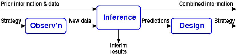
Figure 1: Depiction of one cycle of the three-stage Bayesian adaptive exploration process.

Figures 2 and 3 show highlights of application of BAE to radial velocity (RV) observations of the single-planet system HD 222582. Vogt et al. (2000) reported 24 observations obtained over a 683 d time span with instrumentation at the Keck observatory; Butler et al. (2006) reported 13 subsequent observations. We consider the early observations as a starting point, and compare inferences based on simulated subsequent data at optimal times identified via BAE to inferences using the actual, non-optimal subsequent data (we generated simulated data using the best-fit orbit for all 37 actual observations). Figure 2 shows how the optimal observing time for the first new datum is calculated. Bayesian analysis based on the 24 early data points (red diamonds) produces a posterior distribution for the orbital parameters. We explore the posterior via population-based adaptive Markov chain Monte Carlo sampling, producing an ensemble of possible orbits.

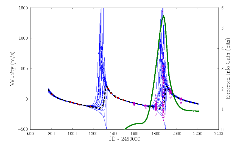
Figure 2: Results based on data from HD 222582: Observed (red diamonds) and predicted (ensemble of thin blue curves; also magenta dots at selected times) velocity vs. time (against left axis); entropy of predictive distribution vs. future observing time (green curve, against right axis).

The blue curves show the velocity curves for 20 posterior samples, roughly depicting the predictive distribution for future data vs. time; the magenta point clouds provide a more complete depiction at selected times, showing $\sim 100$ samples from the predictive distribution at six future times. For this type of data, the expected information gain from future data is proportional to the entropy (uncertainty) in the predictive distribution, so one expects to learn the most by observing where the predictions are most uncertain. The green curve (against the right axis) quantifies this, showing the entropy in the predictive distribution vs. time (in bits relative to repeating the last actual observation), calculated using the predictive distribution samples; its peak identifies the optimal observing time. We generated a single new observation at this time, and repeated the procedure twice more to produce three new optimal observations. The left panel of Figure 3 shows inferences (samples and histograms for marginal distributions) based on the resulting 27 observations; the right panel shows inferences using the 37 actual observations. Inferences with the fewer but optimized new observations are much more precise.

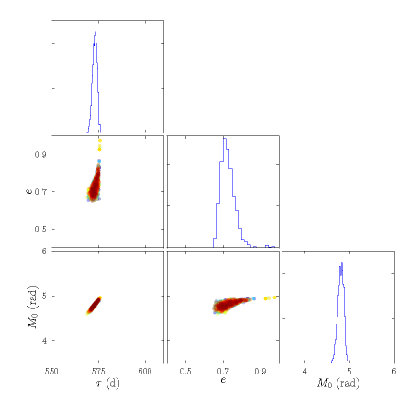
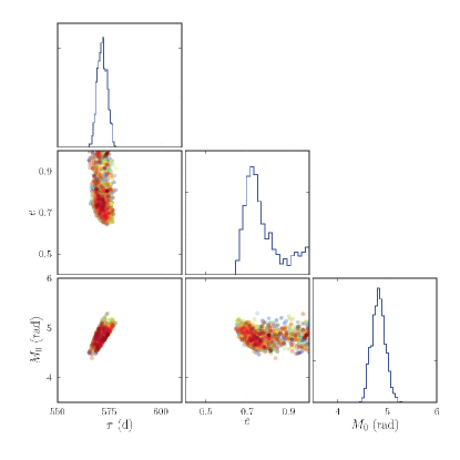
Figure 3: Orbital parameter estimates based on 24 early observations and three simulated new observations at optimal times (left), and based on 24 early and 13 new, non-optimal actual observations (right). Parameters are period, $\tau$, eccentricity, $e$, and mean anomaly at a fiducial time, $M_{0}$.

Beyond Photometric Redshifts using Bayesian Inference

Tamás Budavári
Johns Hopkins University
Baltimore, Maryland, USA

The galaxies in our expanding Universe are seen redder than their actual emission. This redshift in their spectra are typically measured from narrow spectral lines by identifying them to known atomic lines seen in the lab. Spectroscopy provides accurate determinations of the redshift as well as a great insight into the physical processes but is very expensive and time consuming. Alternative methods have been explored for decades. The field of photometric redshifts started when Baum (1962) first compared the magnitudes of red galaxies in distant clusters to local measurements. The first studies were colorful proofs of the concept, which demonstrated the adequate precision of estimating galaxy redshifts based on photometry alone, without spectroscopic follow up. The new field became increasingly important over time, and with the upcoming multicolor surveys just around the corner, the topic is hotter than ever. Traditional methods can be broken down into two distinct classes: empirical and template fitting. Empirical methods rely on training sets of objects with known photometry and spectroscopic redshifts. The usual assumption is that galaxies with the same colors are at identical redshifts. The redshift of a new object is derived based on its vicinity in magnitude space to the calibrators of the training set. Polynomial fitting, locally linear regression and a plethora of other machine learning algorithms have been tested and, usually, with good results. They are easy to implement, fast to run, but are only applicable to new objects with the same photometric measurements in the same regime. Template fitting relies on high-resolution spectral models, which are parameterized by their type, brightness and redshift. The best fitting parameters are typically sought in a maximum likelihood estimation. It is simple to implement and work for new detections in any photometric system but the results are only as good as the template spectra.

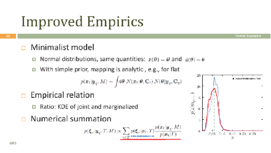
Figure 1: The presented slide illustrates the minimalist model to incorporate the photometric uncertainties of the new galaxy. Using KDE the relation is estimated (blue dotted line), which is averaged with the uncertainty for the final result (red solid line).

To understand the implications of the previous methods and to point toward more advanced approaches, we can use Bayesian inference (Budavári 2009). Constraints on photometric redshifts and other physical parameters in the more general inversion problem are derived from first principles. We combine two key ingredients:

(1) Relation to physics — The redshift (z) is not simply a function of the observables. Considering that they cannot possibly capture all the information, one expects a spread. Regression is only a good model, when the width is very narrow. Otherwise one should estimate the conditional density of $p(z|m)$. While not easy in practice, this is conceptually straightforward to do on a given set of calibrators.

(2) Mapping of the observables — If we would like to perform the estimation of a new object with colors in a separate photometric system, its $m^{\prime}$ magnitudes need to be mapped on to the passbands of the training set (m). This might be as simple as an empirical conversion formula or as sophisticated as spectral synthesis. In general, a model is needed, which can also propagate the uncertainties, $p(m|m^{\prime})$. The final density is the convolution of these two functions.

After 50 years of pragmatism, photometric redshift estimation is now placed on a firm statistical foundation. We can put the traditional methods in context; they are special cases of a unified framework. Their conceptual weaknesses become visible from this aspect. The new approach points us toward more advanced methods that combine the advantages of the earlier techniques. In addition we can formally learn about selecting calibration sets for specific studies. These advancements are going to be vital for analyzing the observations of the next-generation survey telescopes.

Long-Range Climate Forecasts Using Data Clustering and Information Theory

Dimitris Giannakis
New York University
New York, New York, USA

Even though forecasting the weather beyond about two weeks is not possible, certain climate processes (involving, e.g., the large-scale circulation in the Earth’s oceans) are predictable up to a decade in advance. These so-called climate regimes can influence regions as large as the West Coast of North America over several years, and therefore developing models to predict them is a problem of wide practical impact. An additional central issue is to quantify objectively the errors and biases that are invariably associated with these models.

In classical studies on decadal prediction (Boer 2000; 2004, Collins 2002), ensemble experiments are performed using one or more climate models initialized by perturbed initial conditions relative to a reference state, and predictive skill is measured by comparing the root mean square difference of ensemble trajectories to its equilibrium value. However, skill metrics of this type have the drawback of not being invariant under invertible transformations of the prediction variables, and not taking into account the important issue of model error. Further challenges concern the choice of initial conditions of the ensemble members (Hurrell et al. 2009, Meehl et al. 2009, Solomon et al. 2009).

In this talk, we present recent work (Giannakis and Majda 2011a; b) on methods based on data clustering and information theory to build and assess probabilistic models for long-range climate forecasts that address several of the above issues. The fundamental perspective adopted here is that predictions in climate models correspond to transfer of information; specifically transfer of information between the initial conditions (which in general are not known completely) and the state of the climate system at some future time. This opens up the possibility of using the mathematical framework of information theory to characterize both dynamical prediction skill and model error with metrics that are invariant under invertible nonlinear transformations of observables (Kleeman 2002, Roulston and Smith 2002, Majda et al. 2002; 2005, DelSole and Tippet 2007, Majda and Gershgorin 2010).

The key points of our discussion are that (i) the long-range predictive skill of climate models can be revealed through a suitable coarse-grained partition of the set of initial data available to a model (which are generally incomplete); (ii) long-range predictive skill with imperfect models depends simultaneously on the fidelity of these models at asymptotic times, their fidelity during dynamical relaxation to equilibrium, and the discrepancy from equilibrium of forecast probabilities at finite lead times. Here, the coarse-grained partition of the initial data is constructed by data-clustering equilibrium realizations of ergodic dynamical systems without having to carry out ensemble initializations. Moreover, prediction probabilities conditioned on the clusters can be evaluated empirically without having to invoke additional assumptions (e.g., Gaussianity), since detailed initial conditions are not needed to sample these distributions.

In this framework, predictive skill corresponds to the additional information content beyond equilibrium of the cluster-conditional distributions. The natural information-theoretic functional to measure this additional information is relative entropy, which induces a notion of distance between the cluster-conditional and equilibrium distributions. A related analysis leads to measures of model error that correspond to the lack of information (or ignorance) of an imperfect model relative to the true model. The techniques developed here have potential applications across several disciplines involving dynamical system predictions.

As a concrete application of our approach, we study long-range predictability in the equivalent barotropic, double-gyre model of McCalpin and Haidvogel (1996) (frequently called the “1.5-layer model”). This simple model of ocean circulation has non-trivial low-frequency dynamics, characterized by infrequent transitions between meandering, moderate-energy, and extensional configurations of the eastward jet (analogous to the Gulf Stream in the North Atlantic). The algorithm employed here for phase-space partitioning involves building a multi-time family of clusters, computed for different temporal intervals of coarse graining; a recipe similar to kernel density estimation methods. We demonstrate that knowledge of cluster affiliation in the computed partitions carries significant information beyond equilibrium about the total energy and the leading two principal components (PCs) of the streamfunction (which are natural variables for the low-frequency dynamics of this system) for five- to seven-year forecast lead times, i.e., for a timescale about a factor of five longer than the maximum decorrelation time of the PCs.

As an application involving imperfect models, we discuss the error in Markov models of the switching process between the ocean circulation regimes. Imposing Markovianity on the transition process is a familiar approximation in this context (Franzke et al. 2008; 2009), though the validity of this assumption typically remains moot. Our analysis exposes starkly the falseness of predictive skill that one might attribute to a Markovian description of the regime transitions in the 1.5-layer model model by relying on an (internal) assessment based solely on the deviation of the time-dependent prediction probabilities of the Markov model from its biased equilibrium. In particular, we find that a Markov model associated with a seven-state partition appears to outperform a three-state model, both in its discriminating power and its persistence (measured respectively by the deviation from equilibrium and rate of approach to equilibrium), when actually the skill of the seven-state model is false because its equilibrium statistics are biased. Here, the main conclusion is that evaluating simultaneously model errors in both the climatology and the dynamical relaxation to equilibrium should be an integral part of assessments of long-range forecasting skill.

Acknowledgment The material presented in this talk is joint work with Andrew Majda of New York University. This research is partially supported by NSF grant DMS-0456713, from ONR DRI grants N25-74200-F6607 and N00014-10-1-0554, and from DARPA grants N00014-07-10750 and N00014-08-1-1080.

Comparison of Information-Theoretic Methods to estimate the information flow in a dynamical system

Deniz Gencaga
NOAA Crest
New York, New York, USA

Abstract

In order to quantify the amount of information about a variable, or to quantify the information shared between two variables, we utilize information-theoretic quantities like entropy and mutual information (MI), respectively. If these variables constitute a coupled, dynamical system, they share the information along a direction, i.e. we have an information flow in time. In this case, the direction of the information flow also needs to be estimated. However, MI does not provide directionality. Transfer entropy (TE) has been proposed in the literature to estimate the direction of information flow in addition to its magnitude. Here, our goal is to estimate the transfer entropy from observed data accurately. For this purpose, we compare most frequently used methods in the literature and propose our own technique. Unfortunately, every method has its own free tuning parameter(s) so that there is not a consensus on an optimal way of estimating TE from a dataset. In this work, we compare several methods along with a method that we propose, on a Lorenz model. Here, our goal is to develop the required appropriate and reliable mathematical tool synthesizing from all of these disjoint methods used in fields ranging from biomedicine to telecommunications and apply the resulting technique on tropical data sets to better understand events such as the Madden Julian Oscillation in the future.

Introduction and problem statement

Nonlinear coupling between complex dynamical systems is very common in many fields (Wallace et al. 2006, Gourvitch & Eggermont 2007). In order to study the relationships between such coupled subsystems, we must utilize higher-order statistics. Thus, using linear techniques based on correlation analysis cannot be sufficient. Although using mutual information seems to be a good alternative to model higher order nonlinear relationships, it becomes insufficient when we would like to model the directionality of the interactions between the variables, as it is a symmetric measure. Thus, Schrieber (2000), proposed an asymmetric measure between two variables X and Y as follows to study directional interactions:

$${TE}_{{Y}\rightarrow{X}}={T}\left({X}_{i+1}\mid{{\bf X_{i}^{(k)}},{\bf Y_{j}^{(l)}}}\right)=\sum_{i=1}^{N}p\left(x_{x_{i+1}},{\bf x_{i}^{(k)}},{\bf y_{j}^{(l)}}\right)log_{2}\frac{p\left(x_{i+1}\mid{{\bf x_{i}^{(k)}},{\bf y_{j}^{(l)}}}\right)}{p\left(x_{i+1}\mid{{\bf x_{i}^{(k)}}}\right)}$$ (23)

$${TE}_{{X}\rightarrow{Y}}={T}\left({Y}_{i+1}\mid{{\bf Y_{i}^{(k)}},{\bf X_{j}^{(l)}}}\right)=\sum_{i=1}^{N}p\left(y_{y_{i+1}},{\bf y_{i}^{(k)}},{\bf x_{j}^{(l)}}\right)log_{2}\frac{p\left(y_{i+1}\mid{{\bf y_{i}^{(k)}},{\bf x_{j}^{(l)}}}\right)}{p\left(y_{i+1}\mid{{\bf y_{i}^{(k)}}}\right)}$$ (24)

where $x_{i}(k)=[x_{i},\ldots,x_{i-k+1}]$ and $y_{j}(l)=[y_{i},\ldots,y_{i-l+1}]$ are past states and X and Y are $k^{th}$ and $l^{{th}}$ order Markov processes, respectively. Above, ${TE}_{{X}\rightarrow{Y}}$ and ${TE}_{{Y}\rightarrow{X}}$ denote transfer entropies in the direction from X to Y and from Y to X, respectively. For example, in Equation 23, TE describes the degree to which, information about Y allows one to predict future values of X. This is a causal influence that the subsystem Y has on the subsystem X.

Estimation

In the literature, there are a couple of methods to estimate this quantity from data. However, they have their own fine tuning parameters so that there is not a consensus on an optimal way of estimating TE from a dataset. One of them is the Kernel Density Estimation method (Sabesan et al. 2007), where an optimal radius needs to be picked. In another method, called the Adaptive Partitioning of the observation space (Darbellay & Vajda 1999), we make use of the unequal bin sized histograms for mutual information estimations. However, as we have to subtract multivariate mutual information quantities to estimate the final TE, this could be affected by biases. Thus, we propose our own method of generalized Bayesian piecewise-constant model for the probability density function estimation and then calculate TE using the summation formula of individual Shannon entropies.

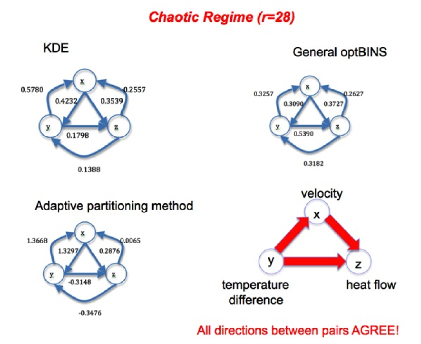
Figure 1: Estimated transfer entropies between the pairs of Lorenz equations using three different methods

EXPERIMENT AND CONCLUSION

We tested three methods on the nonlinear coupled Lorenz equations given below. In climatology, they represent a model of an atmospheric convection roll where x, y, z denote convective velocity, vertical temperature difference and mean convective heat flow, respectively. Using the three methods, we obtained the TE estimates illustrated in Figure 1.

$$\frac{dx}{dt}=\sigma\left({y-x}\right)$$ (25)

$$\frac{dy}{dt}={-xz+rx-y}$$

$$\frac{dz}{dt}={xy-bz}$$

where $\sigma=10$, $b=\frac{8}{3}$, r: Rayleigh number and $r=28$ in a chaotic regime.

In conclusion, computer simulations demonstrate that we can find a reliable parameter regime for all methods at the same time and estimate TE direction from data so that we can identify the information flow between the variables reliably, as all methods agree both mathematically and physically. Currently, we are working on the magnitude differences between the methods so that we can apply TE to identify the information flow between the relevant climate variables of the tropical disturbance, called Madden Julian Oscillation (MJO). Later, this technique will be developed for us to better understand the highly nonlinear nature of atmospheric dynamics.

Reconstructing the Galactic halo’s accretion history: A finite mixture model approach

Duane Lee
Department of Astronomy
Columbia University
New York, New York, USA

Will Jessop
Department of Statistics
Columbia University
New York, New York, USA

Abstract

The stellar halo that surrounds our Milky Way Galaxy is thought to have been built, at least in part, from the agglomeration of stars from many smaller galaxies. This talk outlines an approach to reconstructing the history of Galactic accretion events by looking at the distribution of the chemical abundances of halo stars. The full distribution is assumed to result from the superpositionof stellar populations accreted at different times from progenitor galaxies of different sizes. Our approach uses the Expectation-Maximization (EM) algorithm to find the maximum-likelihood estimators that assess the contribution of each of these progenitors in forming the Galaxy.

Scientific Program

	Thursday, February 24, 2011
10:00	Welcome	Michael Way (GISS)
		Catherine Naud (GISS)
10:20	How long will it take. A historical approach to boundary crossing.	Victor de la Peña (Columbia)
10:45	Cosmology through the Large-Scale Structure of the Universe	Eyal Kazin (NYU)
11:30	On the shoulders of Gauss, Bessel, and Poisson: links, chunks, spheres, and conditional models	William Heavlin (Google)
12:15	Mining Citizen Science Data: Machine Learning Challenges	Kirk Borne (GMU)
13:00	Lunch Break
14:30	Tracking Climate Models: Advances in Climate Informatics	Claire Monteleoni (Columbia)
15:15	Spectral Analysis Methods for Complex Source Mixtures	Kevin Knuth (SUNY/Albany)
16:00	Beyond Objects: Using machines to understand the diffuse universe	Joshua Peek (Columbia)
16:45	Viewpoints: A high-performance visualization and analysis tool	Michael Way (GISS)
	Friday, February 25, 2011
10:00	Clustering Approach for Partitioning Directional Data in Earth and Space Sciences	Christian Klose (Think Geohazards)
10:45	Planetary Detection: The Kepler Mission	Jon Jenkins (NASA/Ames)
11:30	Understanding the possible influence of the solar activity on the terrestrial climate: A times series analysis approach	Elizabeth Martínez-Gómez (Penn State)
12:15	Bayesian adaptive exploration applied to optimal scheduling of exoplanet Radial Velocity observations	Tom Loredo (Cornell)
13:00	Lunch Break
14:30	Bayesian Inference from Photometric Surveys	Tamás Budavári (JHU)
15:15	Long-Range Forecasts Using Data Clustering and Information Theory	Dimitris Giannakis (NYU)
16:00	Comparison of Information-Theoretic Methods to estimate the information flow in a dynamical system	Deniz Gencaga (CCNY)
16:45	Reconstructing the Galactic halo’s accretion history: A finite mixture model approach	Duane Lee and Will Jessop (Columbia)

Participants

Ryan Abrahams	CUNY Graduate Center
Hannah Aizenman	CCNY/Computer Science
Arif Albayrak	NASA GES DISC
Kehinde-Paul Alabi	CCNY/Computer Science
Vivienne Baldassare	CUNY/Hunter College/Physics
Imre Bartos	Columbia/Physics
Mike Bauer	Columbia-NASA/GISS
Rohit Bhardwaj	Columbia/Computer Science
Amitai Bin-Nun	University of Pennsylvania/Astronomy
James Booth	NASA/GISS
Kirk Borne	George Mason University	speaker
Andreas Breiler	IdeLaboratoriet
Douglas Brenner	American Museum of Natural History
Tamas Budavari	Johns Hopkins University	speaker
Samantha Chan	Lamont-Doherty Earth Observatory, Columbia University
Milena C. Cuellar	BCC. CUNY
Victor de al Pena	Columbia/Statistics	speaker
Danielle Dowling	CUNY Graduate Center
Tarek El-Gaaly	Rutgers/Computer Science
Daniel Feldman	CUNY/College of Staten Island
Stephanie Fiorenza	CUNY/College of Staten Island/Physics
Carl Friedberg	NYC/Comets.com
Deniz Gencaga	CCNY/EE, NOAA-CREST	speaker
Dimitrios Giannakis	Center for Atmosphere Ocean Science, Courant Institute of Mathematical Sciences	speaker
Irina Gladkova	CCNY/Computer Science
Elizabeth Gomez	Penn State University/Statistics	speaker
Joshua Gordon	Columbia/Computer Science
Sam Gordon	Columbia
Michael Grossberg	CCNY/Computer Science

Participants cont’

Michael Haken	NASA/GSFC, Science Systems & Applications, Inc.
Zachary Haberman	SUNY at Albany/Physics
Naveed Hasan	Columbia/Computer Science
Nicholas Hatzopoulos	CUNY Gradate Center
William D Heavlin	Google, Inc	speaker
Kay Hiranaka	CUNY Graduate Center
Hao Huang	Stony Brook University/Computer Science
Darryl Hutchinson	CUNY Graduate Center
Ilknur Icke	CUNY Graduate Center/Computer Science
Geetha Jagannathan	Columbia/Computer Science
Jon Jenkins	SETI Institute/NASA Ames Research Center	speaker
Will Jessop	Columbia/Statistics	speaker
Ed Kaita	SSAI@GSFC/NASA
Eyal Kazin	New York University	speaker
Lee Case Klippel	Columbia University
Christian D. Klose	Think GeoHazards	speaker
Kirk Knobelspiesse	ORAU-NASA/GISS
Kevin Knuth	SUNY at Albany	speaker
Ioannis Kostopoulos	CUNY Graduate Center
Duane Lee	Columbia/Astronomy	speaker
Erbo Li	Columbia/Computer Science
Charles Liu	CUNY at CSI
Thomas Loredo	Cornell/Astronomy	speaker
Chris Malone	SUNY at Stony Brook/Physics and Astronomy
Szabolcs Marka	Columbia/Physics
Zsuzsa Marka	Columbia Astrophysics Laboratory
Haley Maunu	SUNY at Albany/Physics
Vinod Mohan	Columbia
Claire Monteleoni	Columbia/Computer Science	speaker

Participants cont’

Catherine Naud	NASA/GISS
Alejandro Nunez	CUNY Graduate Center
Indrani Pal	IRI, The Earth Institute
Vladimir Pavlovic	Rutgers/Computer Science
Joshua Peek	Columbia/Astronomy	speaker
Fergie Ramos	Student/College of New Rochelle
Khary Richardson	CUNY Graduate Center
William Rossow	CCNY/NOAA-CREST
Syamantak Saha	NYU Stern
Destry Saul	Columbia/Astronomy
Joshua Schlieder	SUNY at Stony Brook
Frank Scalzo	NASA/GISS
Bodhisattva Sen	Columbia/Statistics
Monika Sikand	Stevens Institute of Tech/Physics
Michal Simon	SUNY at Stony Brook/Physics and Astronomy
Ishan Singh	Columbia
Damain Sowinski	CUNY Graduate Center
Ilya Tsinis	NYU/Courant
Maria Tzortziou	GSFC/NASA - University of Maryland
Michael Way	NASA/GISS
Adrian Weller	Columbia/Computer Science
Laird Whitehill	Cornell/Astronomy
Alexander Wong	JP Morgan Chase
Nettie Wong	American Museum of Natural History
Emmi Yonekura	Columbia University
Shinjae Yoo	Brookhaven National Lab/Computer Science Center
Sejong Yoon	Rutgers/Computer Science
Dantong Yu	Brookhaven National Lab

Video Links

Introduction	Michael Way
http://www.youtube.com/watch?v=CHEoya_e2Do	(NASA/GISS)
How long will it take. A historical approach to boundary crossing	Victor de la Peña
http://www.youtube.com/watch?v=3gfHeerVqHs	(Columbia U)
Cosmology through the Large-Scale Structure of the Universe	Eyal Kazin
http://www.youtube.com/watch?v=es4dH0jBJYw	(NYU)
On the shoulders of Gauss, Bessel, and Poisson: links, chunks, spheres, and conditional models	William Heavlin
http://www.youtube.com/watch?v=FzFAxaXTkUQ	(Google Inc.)
Mining Citizen Science Data: Machine Learning Challenges	Kirk Borne
http://www.youtube.com/watch?v=XoS_4axsb5A	(GMU)
Tracking Climate Models: Advances in Climate Informatics	Claire Monteleoni
http://www.youtube.com/watch?v=78IeffwV6bU	(Columbia U)
Spectral Analysis Methods for Complex Source Mixtures	Kevin Knuth
http://www.youtube.com/watch?v=t9mCoff5YZo	(Suny/Albany)
Beyond Objects: Using machines to understand the diffuse universe	Joshua Peek
http://www.youtube.com/watch?v=hgp8CeR43So	(Columbia U)
Viewpoints: A high-performance visualization and analysis tool	Michael Way
http://www.youtube.com/watch?v=FsW64idYw6c	(NASA/GISS)
Clustering Approach for Partitioning Directional Data in Earth and Space Sciences	Christian Klose
http://www.youtube.com/watch?v=5Ak6_rvayqg	(Think Geohazards)
Planetary Detection: The Kepler Mission	Jon Jenkins
http://www.youtube.com/watch?v=2dnA95smRE0	(NASA/Ames)
Understanding the possible influence of the solar activity on the terrestrial climate: A times series analysis approach	Elizabeth Martínez-Gómez
http://www.youtube.com/watch?v=CXmC1dh9Wdg	(Penn State)
Bayesian adaptive exploration applied to optimal scheduling of exoplanet Radial Velocity observations	Tom Loredo
http://www.youtube.com/watch?v=B1pVtHmu9E0	(Cornell U)
Bayesian Inference from Photometric Surveys	Tamas Budavari
http://www.youtube.com/watch?v=xCzUl0HtWGM	(JHU)
Long-Range Forecasts Using Data Clustering and Information Theory	Dimitris Giannakis
http://www.youtube.com/watch?v=pFDqP94btCg	(NYU)
Comparison of Information-Theoretic Methods to estimate the information flow in a dynamical system	Deniz Gencaga
http://www.youtube.com/watch?v=ejX_MWImP6A	(CCNY)
Reconstructing the Galactic halo’s accretion history:	Duane Lee &
A finite mixture model approach	Will Jessop
http://www.youtube.com/watch?v=moehYYsIOFw	(Columbia U)

References

- Baranuik (2011) Baranuik, R.G. 2011, More Is Less: Signal Processing and the Data Deluge, Science, 331, 6018, 717
- Foster et al. (2009) Foster, L., Waagen, A., Aijaz, N., Hurley, M., Luis, A., Rinsky, J. Satyavolu, C., Way, M., Gazis, P., Srivastava, A. 2009, Stable and Efficient Gaussian Process Calculations, Journal of Machine Learning Research, 10, 857
- Fox & Hendler (2011) Fox, P. & Hendler, J. 2011, Changing the Equation on Scientific Data Visualization, Science, 331, 6018, 705
- Gazis, Levit, & Way (2010) Gazis, P.R., Levit, C. & Way, M.J. 2010, Viewpoints: A High-Performance High-Dimensional Exploratory Data Analysis Tool, Publications of the Astronomical Society of the Pacific, 122, 1518
- Hastie, Tibshirani, & Friedman (2003) Hastie, T., Tibshirani, R. & Friedman, J.H. 2003, The Elements of Statistical Learning, Springer 2003, ISBN-10: 0387952845
- Hey et al. (2009) Hey, T., Tansley, S. & Tolle, K. 2009, The Fourth Paradigm: Data-Intensive Scientific Discovery, Microsoft Research, ISBN-10: 0982544200
- Morris (2010) Morris, I. 2010, Why the West Rules–for Now: The Patterns of History, and What They Reveal About the Future, Farrar, Straus and Giroux, ISBN-10: 0374290024
- Way et al. (2009) Way, M.J., Foster, L.V., Gazis, P.R. & Srivastava, A.N. 2009, New Approaches To Photometric Redshift Prediction Via Gaussian Process Regression In The Sloan Digital Sky Survey, The Astrophysical Journal, 706, 623
- Way et al. (2011) Way, M.J., Scargle, J., Ali, K & Srivastava, A.N. 2011, Advances in Machine Learning and Data Mining for Astronomy, in preparation, Chapman and Hall

References

- Brown et al. (2011) Brown M, de la Peña, V.H., Kushnir, Y & Sit, T 2011, “On Estimating Threshold Crossing Times,” submitted.
- Seager et al. (2007) Seager, R., Ting, M. F., Held, I., Kushnir, Y., Lu, J., Vecchi, G., Huang, H. P., Harnik, N., Leetmaa, A., Lau, N. C., Li, C. H., Velez, J. & Naik, N. 2007, “Model projections of an imminent transition to a more arid climate in southwestern North America,” Science, May 25, Volume 316, Issue 5828, p.1181-1184.
- Randall et al. (2007) Randall D.A., Wood R.A., Bony S., Colman R., Fichefet T., Fyfe J., Kattsov V., Pitman A., Shukla J., Srinivasan J., Stouffer R.J., Sumi A. & Taylor K.E. 2007, “Climate Models and Their Evaluation.” in: Climate Change 2007: The Physical Science Basis. Contribution of Working Group I to the Fourth Assessment Report of the Intergovernmental Panel on Climate Change, Solomon, S, Qin D, Manning M, Chen Z, Marquis M, Averyt KB, Tignor M, Miller HL, editors. Cambridge University Press, Cambridge, United Kingdom and New York, NY, USA.

References

- Clowe et al. (2004) Clowe, D., Gonzalez, A., & Markevitch, M. 2004, The Astrophysical Journal, 604, 596
- Eisenstein et al. (2011) Eisenstein, D. J., Weinberg, D. H., Agol, E., Aihara, H., Allende Prieto, C., Anderson, S. F., Arns, J. A., Aubourg, E., Bailey, S., Balbinot, E., et al. 2011, arXiv:1101.1529v1
- Eisenstein et al. (2001) Eisenstein, D. J. et al. 2001, The Astronomical Journal, 122, 2267
- Eisenstein et al. (2005) Eisenstein, D. J. et al. 2005, The Astrophysical Journal, 633, 560
- Kazin et al. (2010) Kazin, E. A., Blanton, M. R., Scoccimarro, R., McBride, C. K., Berlind, A. A., Bahcall, N. A., Brinkmann, J., Czarapata, P., Frieman, J. A., Kent, S. M., Schneider, D. P., & Szalay, A. S. 2010, The Astrophysical Journal, 710, 1444
- Komatsu et al. (2009) Komatsu, E., Dunkley, J., Nolta, M. R., Bennett, C. L., Gold, B., Hinshaw, G., Jarosik, N., Larson, D., Limon, M., Page, L., Spergel, D. N., Halpern, M., Hill, R. S., Kogut, A., Meyer, S. S., Tucker, G. S., Weiland, J. L., Wollack, E., & Wright, E. L. 2009, The Astrophysical Journal Supplement Series, 180, 330
- Landy & Szalay (1993) Landy, S. D. & Szalay, A. S. 1993, The Astrophysical Journal, 412, 64
- Larson et al. (2011) Larson, D., Dunkley, J., Hinshaw, G., Komatsu, E., Nolta, M. R., Bennett, C. L., Gold, B., Halpern, M., Hill, R. S., Jarosik, N., Kogut, A., Limon, M., Meyer, S. S., Odegard, N., Page, L., Smith, K. M., Spergel, D. N., Tucker, G. S., Weiland, J. L., Wollack, E., & Wright, E. L. 2011, The Astrophysical Journal Supplement Series, 192, 16
- Penzias & Wilson (1965) Penzias, A. A. & Wilson, R. W. 1965, The Astrophysical Journal, 142, 419
- Percival et al. (2010) Percival, W. J., Reid, B. A., Eisenstein, D. J., Bahcall, N. A., Budavari, T., Fukugita, M., Gunn, J. E., Ivezic, Z., Knapp, G. R., Kron, R. G., Loveday, J., Lupton, R. H., McKay, T. A., Meiksin, A., Nichol, R. C., Pope, A. C., Schlegel, D. J., Schneider, D. P., Spergel, D. N., Stoughton, C., Strauss, M. A., Szalay, A. S., Tegmark, M., Weinberg, D. H., York, D. G., & Zehavi, I. 2010, Monthly Notices of the Royal Astronomical Society, 401, 2148
- Perlmutter et al. (1999) Perlmutter, S. et al. 1999, The Astrophysical Journal, 517, 565
- Riess et al. (1998) Riess, A. G., Filippenko, A. V., Challis, P., Clocchiatti, A., Diercks, A., Garnavich, P. M., Gilliland, R. L., Hogan, C. J., Jha, S., Kirshner, R. P., Leibundgut, B., Phillips, M. M., Reiss, D., Schmidt, B. P., Schommer, R. A., Smith, R. C., Spyromilio, J., Stubbs, C., Suntzeff, N. B., & Tonry, J. 1998, The Astronomical Journal, 116, 1009
- Rubin & Ford (1970) Rubin, V. C. & Ford, Jr., W. K. 1970, The Astrophysical Journal, 159, 379
- SDSS-III collaboration: Hiroaki Aihara et al. (2011) SDSS-III collaboration: Hiroaki Aihara, Allende Prieto, C., An, D., et al. 2011, arXiv:1101.1559v2
- Smoot et al. (1992) Smoot, G. F., Bennett, C. L., Kogut, A., Wright, E. L., Aymon, J., Boggess, N. W., Cheng, E. S., de Amici, G., Gulkis, S., Hauser, M. G., Hinshaw, G., Jackson, P. D., Janssen, M., Kaita, E., Kelsall, T., Keegstra, P., Lineweaver, C., Loewenstein, K., Lubin, P., Mather, J., Meyer, S. S., Moseley, S. H., Murdock, T., Rokke, L., Silverberg, R. F., Tenorio, L., Weiss, R., & Wilkinson, D. T. 1992, The Astrophysical Journal Letters, 396, L1
- Torbet et al. (1999) Torbet, E., Devlin, M. J., Dorwart, W. B., Herbig, T., Miller, A. D., Nolta, M. R., Page, L., Puchalla, J., & Tran, H. T. 1999, The Astrophysical Journal Letters, 521, L79
- Zwicky (1933) Zwicky, F. 1933, Helvetica Physica Acta, 6, 110

References

- Fan & Lv (2008) Fan, J. & Lv, J. 2008, “Sure independence screening for ultra-high dimensional feature space (with discussion).” Journal of the Royal Statistical Society, series B vol. 70, pp. 849-911.
- Jorgensen (2006) Jorgensen, M. (2006). “Iteratively reweighted least squares,” Encyclopedia of Environmetrics. John Wiley & Sons.
- McCullough & Nelder (1999) McCullough, P. & Nelder, J.A. 1999, Generalized Linear Models, 2nd edition, John Wiley & Sons.
- Mardia & Jupp (2000) Mardia, K.V. & Jupp, P.E. 2000, Directional Statistics, 2nd edition, John Wiley & Sons.
- Plis et al. (2010) Plis, S.M., Lane, T., Calhoun, V.D. 2010, “Permutations as angular data: efficient inference in factorial spaces,” IEEE International Conference on Data Mining, pp.403-410.
- Schapire & Singer (1999) Schapire, R.E. & Singer, Y. 1999, “Improved Boosting Algorithms Using Confidence-Rated Predictors.” Machine Learning, vol. 37, pp. 297-336.
- Watson & Williams (1956) Watson, G.S. & Williams, E.J. 1956, “On the construction of significance tests on the circle and the sphere.” Biometrika, vol. 43. pp. 344-352.

References

- Baehr (2010) Baehr, S., Vedachalam, A., Borne, K., & Sponseller, D., ”Data Mining the Galaxy Zoo Mergers,” NASA Conference on Intelligent Data Understanding, https://c3.ndc.nasa.gov/dashlink/resources/220/, pp. 133-144 (2010).

References

- Monteleoni & Jaakkola (2003) Monteleoni, C. & Jaakkola, T. 2003 “Online learning of non-stationary sequences”, In NIPS ’03: Advances in Neural Information Processing Systems 16, 2003
- Monteleoni, Schmidt & Saroha (2010) Monteleoni, C., Schmidt, G & Saroha, S. 2010 “Tracking Climate Models”, in NASA Conference on Intelligent Data Understanding, 2010

References

- Knuth (2005) Knuth, K.H. 2005. “Informed source separation: A Bayesian tutorial” (Invited paper) B. Sankur , E. Çetin, M. Tekalp , E. Kuruoğlu (ed.), Proceedings of the 13th European Signal Processing Conference (EUSIPCO 2005), Antalya, Turkey.
- Knuth et al. (2007) Knuth, K.H., Tse M.K., Choinsky J., Maunu H.A, Carbon D.F. 2007, “Bayesian source separation applied to identifying complex organic molecules in space”, Proceedings of the IEEE Statistical Signal Processing Workshop, Madison WI, August 2007.
- Nathan (2010) Nathan, B. 2010. “Spectral analysis methods for characterizing organic molecules in space”. M.S. Thesis, University at Albany, K.H. Knuth, Advisor.

References

- Begum et al. (2010) Begum, A., Stanimirovic, S., Peek, J. E., Ballering, N. P., Heiles, C., Douglas, K. A., Putman, M., Gibson, S. J., Grcevich, J., Korpela, E. J., Lee, M.-Y., Saul, D., & Gallagher, J. S. 2010, eprint arXiv, 1008, 1364
- Chepurnov et al. (2010) Chepurnov, A., Lazarian, A., Stanimirović, S., Heiles, C., & Peek, J. E. G. 2010, The Astrophysical Journal, 714, 1398
- Ford et al. (2010) Ford, H. A., Lockman, F. J., & McClure-Griffiths, N. M. 2010, The Astrophysical Journal, 722, 367
- Hanisch (2010) Hanisch, R. 2010, Astronomical Data Analysis Software and Systems XIX, 434, 65
- Heiles (1979) Heiles, C. 1979, Astrophysical Journal, 229, 533
- Kim et al. (1998) Kim, S., Staveley-Smith, L., Dopita, M. A., Freeman, K. C., Sault, R. J., Kesteven, M. J., & Mcconnell, D. 1998, Astrophysical Journal v.503, 503, 674
- Kulkarni & Heiles (1988) Kulkarni, S. R. & Heiles, C. 1988, Neutral hydrogen and the diffuse interstellar medium, 95–153
- Lang et al. (2010) Lang, D., Hogg, D. W., Mierle, K., Blanton, M., & Roweis, S. 2010, The Astronomical Journal, 139, 1782
- Lupton et al. (2001) Lupton, R., Gunn, J. E., Ivezic, Z., Knapp, G. R., Kent, S., & Yasuda, N. 2001, arXiv, astro-ph
- McClure-Griffiths et al. (2006) McClure-Griffiths, N. M., Dickey, J. M., Gaensler, B. M., Green, A. J., & Haverkorn, M. 2006, The Astrophysical Journal, 652, 1339
- Peek et al. (2011) Peek, J. E. G., Heiles, C., Douglas, K. A., Lee, M.-Y., Grcevich, J., Stanimirovic, S., Putman, M. E., Korpela, E. J., Gibson, S. J., Begum, A., & Saul, D. 2011, The Astrophysical Journal Supplement, 1
- Saul et al. (2011) Saul, D., Peek, J. E. G., Grcevich, J., & Putman, M. E. 2011, in prep, 1
- Sonka et al. (2008) Sonka, M., Hlavac, V., & Boyle, R. 2008, 829
- West et al. (2010) West, A. A., Garcia-Appadoo, D. A., Dalcanton, J. J., Disney, M. J., Rockosi, C. M., Ivezić, Ž., Bentz, M. C., & Brinkmann, J. 2010, The Astronomical Journal, 139, 315
- York et al. (2000) York, D. G., Adelman, J., Anderson, J., Anderson, S. F., Annis, J., Bahcall, N. A., Bakken, J. A., Barkhouser, R., Bastian, S., Berman, E., Boroski, W. N., Bracker, S., Briegel, C., Briggs, J. W., Brinkmann, J., Brunner, R., Burles, S., Carey, L., Carr, M. A., Castander, F. J., Chen, B., Colestock, P. L., Connolly, A. J., Crocker, J. H., Csabai, I., Czarapata, P. C., Davis, J. E., Doi, M., Dombeck, T., Eisenstein, D., Ellman, N., Elms, B. R., Evans, M. L., Fan, X., Federwitz, G. R., Fiscelli, L., Friedman, S., Frieman, J. A., Fukugita, M., Gillespie, B., Gunn, J. E., Gurbani, V. K., de Haas, E., Haldeman, M., Harris, F. H., Hayes, J., Heckman, T. M., Hennessy, G. S., Hindsley, R. B., Holm, S., Holmgren, D. J., h Huang, C., Hull, C., Husby, D., Ichikawa, S.-I., Ichikawa, T., Ivezić, Ž., Kent, S., Kim, R. S. J., Kinney, E., Klaene, M., Kleinman, A. N., Kleinman, S., Knapp, G. R., Korienek, J., Kron, R. G., Kunszt, P. Z., Lamb, D. Q., Lee, B., Leger, R. F., Limmongkol, S., Lindenmeyer, C., Long, D. C., Loomis, C., Loveday, J., Lucinio, R., Lupton, R. H., MacKinnon, B., Mannery, E. J., Mantsch, P. M., Margon, B., McGehee, P., McKay, T. A., Meiksin, A., Merelli, A., Monet, D. G., Munn, J. A., Narayanan, V. K., Nash, T., Neilsen, E., Neswold, R., Newberg, H. J., Nichol, R. C., Nicinski, T., Nonino, M., Okada, N., Okamura, S., Ostriker, J. P., Owen, R., Pauls, A. G., Peoples, J., Peterson, R. L., Petravick, D., Pier, J. R., Pope, A., Pordes, R., Prosapio, A., Rechenmacher, R., Quinn, T. R., Richards, G. T., Richmond, M. W., Rivetta, C. H., Rockosi, C. M., Ruthmansdorfer, K., Sandford, D., Schlegel, D. J., Schneider, D. P., Sekiguchi, M., Sergey, G., Shimasaku, K., Siegmund, W. A., Smee, S., Smith, J. A., Snedden, S., Stone, R., Stoughton, C., Strauss, M. A., Stubbs, C., SubbaRao, M., Szalay, A. S., Szapudi, I., Szokoly, G. P., Thakar, A. R., Tremonti, C., Tucker, D. L., Uomoto, A., Berk, D. V., Vogeley, M. S., Waddell, P., i Wang, S., Watanabe, M., Weinberg, D. H., Yanny, B., & Yasuda, N. 2000, The Astronomical Journal, 120, 1579

References

- Gazis et al. (2010) Gazis, P.R., Levit, C. & Way, M.J. 2010, Publications of the Astronomical Society of the Pacific, 122, 1518, “Viewpoints: A High-Performance High-Dimensional Exploratory Data Analysis Tool”
- Sandstrom et al. (2003) Sandstrom, T. A., Henze, C. & Levit, C. 2003, Coordinated & Multiple Views in Exploratory Visualization, (Piscataway: IEEE), 124

References

- Anderberg (1973) Anderberg M. R., Cluster analysis for applications. 1973; Academic Press.
- Dershowitz et al. (1996) Dershowitz W. Busse R. Geier J. and Uchida M., A stochastic approach for fracture set definition, In: Aubertin M. Hassani F. and Mitri H., eds., Proc., 2nd NARMS, Rock Mechanics Tools and Techniques, Montreal. 1996; 1809-1813.
- Fisher et al. (1987) Fisher, N. I. Lewis, T. and Embleton B. J., Statistical analysis of spherical data. 1987; Cambridge University Press.
- Fukunaga (1990) Fukunaga K., Introduction to statistical pattern recognition. 1990; Academic Press.
- Gray (1984) Gray R.M., Vector Quantization, IEEE ASSP. 1984; 1 (2): 4-29.
- Hammah & Curran (1998) Hammah R. E. and Curran J. H., Fuzzy cluster algorithm for the automatic delineation of joint sets, Int. J. Rock Mech. Min. Sci. 1998; 35 (7): 889-905.
- Klose (2004) Klose R.M., A New Clustering Approach for Partiontioning Directional Data, IJRMMS. 2004; (42): 315-321.
- Pecher (1989) Pecher A., SchmidtMac - A program to display and analyze directional data, Computers & Geosciences. 1989; 15 (8): 1315-1326.
- Robbins & Monro (1951) Robbins H. and Monro S., A stochastic approximation method, Ann. Math. Stat. 1951; 22: 400-407.
- Schmidt (1925) Schmidt W., Gefügestatistik, Tschermaks Mineral. Petrol. Mitt. 1925; 38: 392-423.
- Shanley & Mahtab (1976) Shanley R. J. and Mahtab M. A., Delineation and analysis of clusters in orientation data, Mathematical Geology. 1976; 8 (1): 9-23.
- Wallbrecher (1978) Wallbrecher E., Ein Cluster-Verfahren zur richungsstatistischen Analyse tektonischer Daten, Geologische Rundschau. 1978; 67 (3): 840-857.

References

- Dingel & Landberg (1971) Dingle, A. N. & H. E. Landsberg 1971, Science, 173(3995), 461-462.
- Laken et al. (2010) Laken, B. A., D. R. Kniveton and M. R. Frogley 2010, Atmos. Chem. Phys., 10, 10941–10948.
- Lean et al. (1995) Lean, J., J. Beer and R. Bradley (1995), Geophys. Res. Lett., 22(23), 3195-3198.
- Lütkepohl (1993) Lütkepohl, H. 1993, Introduction to multiple time series analysis, Springer Verlag, Germany.
- Schneider (1979) Schneider, S. H. (1979), The effect of man’s activities on climatic changes in Evolution of Planetary and Climatology of the Earth. Proceedings of the International Conference, Nice, France, 16-20 October 1978, pp. 527.
- Sims (1972) Sims, C. A. 1972, American Economic Review 62, 540-552.
- Sims (1980) Sims, C. A. 1980, Econometrica 48, 1-48.
- Sims (1982) Sims, C. A. 1982, Brooking Papers on Economic Activity 1, 107-152.
- Tett et al. (1999) Tett, F. B. S., P. A. Stott, M. R. Allen, W. J. Ingram & J. F. B. Mitchell 1999, Nature, 399, 569-572.
- Willett (1949) Willett, H. C. 1949, J. Atm. Sciences, 6(1), 34-50.

References

- Vogt et al. (2000) Vogt, S.S., Marcy, G.W., Butler, R.P. & Apps, K. 2000, Six New Planets from the Keck Precision Velocity Survey, Astrophysical Journal, 536, 902
- Butler et al. (2006) Butler, R. P., Wright, J. T., Marcy, G. W., Fischer, D. A., Vogt, S. S., Tinney, C. G., Jones, H. R. A., Carter, B. D., Johnson, J. A., McCarthy, C. & Penny, A. J. 2006, Catalog of Nearby Exoplanets, Astrophysical Journal, 646, 505

References

- Boer (2000) G. J. Boer. A study of atmosphere-ocean predictability on long time scales. Climate Dyn., 16(6):469–477, 2000. doi: 10.1007/s003820050340.
- Boer (2004) G. J. Boer. Long time-scale potential predictability in an ensemble of coupled climate models. Climate Dyn., 23(1):29–44, 2004. doi: 10.1007/s00382-004-0419-8.
- Collins (2002) M. Collins. Climate predictability on interannual to decadal time scales: The initial value problem. Climate Dyn., 19:671–692, 2002. doi: 10.1007/s00382-002-0254-8.
- DelSole and Tippet (2007) T. DelSole and M. K. Tippet. Predictability: Recent insights from information theory. Rev. Geophys., 45:RG4002, 2007. doi: 10.1029/2006rg000202.
- Franzke et al. (2008) C. Franzke, D. Crommelin, A. Fischer, and A. J. Majda. A hidden Markov model perspective on regimes and metastability in atmospheric flows. J. Climate, 21(8):1740–1757, 2008. doi: 10.1175/2007jcli1751.1.
- Franzke et al. (2009) C. Franzke, I. Horenko, A. J. Majda, and R. Klein. Systematic metastable regime identification in an AGCM. J. Atmos. Sci., 66(9):1997–2012, 2009. doi: 10.1175/2009jas2939.1.
- Giannakis and Majda (2011a) D. Giannakis and A. J. Majda. Quantifying the predictive skill in long-range forecasting. Part I: Coarse-grained predictions in a simple ocean model. J. Climate, 2011a. submitted.
- Giannakis and Majda (2011b) D. Giannakis and A. J. Majda. Quantifying the predictive skill in long-range forecasting. Part II: Model error in coarse-grained Markov models with application to ocean-circulation regimes. J. Climate, 2011b. submitted.
- Hurrell et al. (2009) J. W. Hurrell et al. Decadal climate prediction: Opportunities and challenges. In Proceedings of the OceanObs09 Conference: Sustained Ocean Observations and Information for Society, pages 21–25, Venice, Italy, 2009.
- Kleeman (2002) R. Kleeman. Measuring dynamical prediction utility using relative entropy. J. Atmos. Sci., 59(13):2057–2072, 2002.
- Majda and Gershgorin (2010) A. J. Majda and B. Gershgorin. Quantifying uncertainty in climage change science through empirical information theory. Proc. Natl. Acad. Sci., 107(34):14958–14963, 2010. doi: 10.1073/pnas.1007009107.
- Majda et al. (2002) A. J. Majda, R. Kleeman, and D. Cai. A mathematical framework for predictability through relative entropy. Methods Appl. Anal., 9(3):425–444, 2002.
- Majda et al. (2005) A. J. Majda, R. V. Abramov, and M. J. Grote. Information Theory and Stochastics for Multiscale Nonlinear Systems, volume 25 of CRM Monograph Series. Americal Mathematical Society, Providence, 2005.
- McCalpin and Haidvogel (1996) J. D. McCalpin and D. B. Haidvogel. Phenomenology of the low-frequency variability in a reduced-gravity quasigeostrophic double-gyre model. J. Phys. Oceanogr., 26(5):739–752, 1996.
- Meehl et al. (2009) G. A. Meehl et al. Decadal prediction. can it be skillful? Bull. Amer. Meteor. Soc., 90(10):1467–1485, 2009. doi: 10.1175/2009bams2778.1.
- Roulston and Smith (2002) M.S. Roulston and L.A. Smith. Evaluating probabilistic forecasts using information theory. Mon. Weather Rev., 130(6):1653–1660, 2002.
- Solomon et al. (2009) A. Solomon et al. Distinguishing the roles of natural and anthropogenically forced decadal climate variability: Implications for prediction. Bull. Amer. Meteor. Soc., 2009. Submitted.

References

- Wallace et al. (2006) J. Wallace, P. Hobbs, Atmospheric Science, Second Edition: An Introductory Survey, 2006
- Gourvitch & Eggermont (2007) B. Gourvitch and J. Eggermont, “Evaluating Information Transfer Between Auditory Cortical Neurons”, J. Neurophysiology, vol. 97, no.3, pp. 2533-2543.
- Schrieber (2000) T. Schreiber, “Measuring information transfer”, Phys. Rev. Let., Vol. 85, No. 2, pp.461-464, 2000
- Sabesan et al. (2007) S. Sabesan, K. Narayanan, A. Prasad, L. Iasemidis, A. Spanias and K. Tsakalis, “Information Flow in Coupled Nonlinear Systems: Application to the Epileptic Human Brain”, Data Mining in Biomedicine, Data Mining in Biomedicine, 2007
- Darbellay & Vajda (1999) G. Darbellay and I. Vajda, “Estimation of the Information by an adaptive partitioning of the observation space”, IEEE Trans. On Information Theory, Vol. 45, No.4, 1999