A local limit theorem for the minimum of a random walk with markovian increasements

Yinna YE ⁽⁾

Abstract. Let $(\Omega,\mathcal{F},\mathbb{P})$ be a probability space and $E$ be a finite set. Assume that $X=(X_{n})$ is an irreducible and aperiodic Markov chain, defined on $(\Omega,\mathcal{F},\mathbb{P})$, with values in $E$ and with transition probability $\displaystyle P=\Big{(}p_{i,j}\Big{)}_{i,j}$. Let $(F(i,j,\text{d}x))_{i,j\in E}$ be a family of probability measures on $\mathbb{R}$. Consider a semi-markovian chain $(Y_{n},X_{n})$ on $\mathbb{R}\times E$ with transition probability $\widetilde{P}$, defined by $\displaystyle\widetilde{P}\Big{(}(u,i),A\times\{j\}\Big{)}=\mathbb{P}(Y_{n+1}\in A,X_{n+1}=j|\,Y_{n}=u,\,X_{n}=i)=p_{i,j}\,F(i,j,A)$, for any $(u,i)\in\mathbb{R}\times E$, any Borel set $A\subset\mathbb{R}$ and any $j\in E$. We study the asymptotic behavior of the sequence of Laplace transforms of $(X_{n},m_{n})$, where $m_{n}=\min(S_{0},S_{1},\cdots,S_{n})$ and $S_{n}=Y_{0}+\cdots+Y_{n-1}$. Under quite general assumptions on $F(i,j,\text{d}x)$, we prove that for all $(i,j)\in E\times E$, $\sqrt{n}\;\mathbb{E}_{i}[\exp(\lambda m_{n}),X_{n}=j]$ converges to a positive function $H_{i,j}(\lambda)$ and we obtain further information on this limit function as $\lambda\rightarrow 0^{+}$.

This is the second version of ”A local limit theorem for the minimum of a random walk with markovian increasements” (Apr. 2011, arXiv:1104.1554v1). In this version, author’s present address is updated, typos are corrected and some notations are unified.

1 Introduction and main results

Let $(\Omega,\mathcal{F},\mathbb{P})$ be a probability space and $E$ be a finite set with $N$ elements. Assume that $X=(X_{n})_{n\geq 0}$ is an irreducible and aperiodic Markov chain, defined on $(\Omega,\mathcal{F},\mathbb{P})$, with values in $E$ and with transition probability $P=\Big{(}p_{i,j}\Big{)}_{i,j\in E}$. The chain $X$ admits a unique invariant probability denoted by $\nu$. Let $\displaystyle(F(i,j,\text{d}t))_{i,j\in E}$ be a family of probability measures on $\mathbb{R}$. Consider a sequence of $\mathbb{R}$-valued random variables $(Y_{n})_{n\geq 0}$ defined on $(\Omega,\mathcal{F},\mathbb{P})$, such that $(Y_{n},X_{n})_{n\geq 0}$ is a Markov chain on $\mathbb{R}\times E$ with transition probability $\widetilde{P}$, defined by:
for any $(x,i)\in\mathbb{R}\times E$, any Borel set $A\subset\mathbb{R}$ and $j\in E$,

$$\widetilde{P}\Big{(}(u,i),A\times\{j\}\Big{)}=\mathbb{P}(Y_{n+1}\in A,X_{n+1}=j|\,Y_{n}=u,\,X_{n}=i)=p_{i,j}\,F(i,j,A).$$

Such a chain $(Y_{n},X_{n})_{n\geq 0}$ is called a semi-markovian chain: once the family $\displaystyle(F(i,j,\cdot))_{i,j\in E}$ is fixed, the transitions of this chain is controlled by $(X_{n})_{n\geq 0}$. We thus consider the canonical probability space $\displaystyle\Big{(}(\mathbb{R}\times E)^{\mathbb{N}},\Bigl{(}\mathcal{B}(\mathbb{R})\otimes\mathcal{P}(E)\Big{)}^{\otimes\mathbb{N}},(\mathbb{P}_{(u,i)})_{(u,i)\in\mathbb{R}\times E}\Big{)}$ associated with $(Y_{n},X_{n})_{n\geq 0}$ and, for any $(u,i)\in\mathbb{R}\times E$, we denoted by $\mathbb{E}_{(u,i)}$ the expectation with respect to $\mathbb{P}_{(u,i)}$. To simplify our notations, we will denote $\mathbb{P}_{(0,i)}$ by $\mathbb{P}_{i}$ and $E_{(0,i)}$ by $\mathbb{E}_{i}$.

Set $S_{0}=0,S_{n}=S_{0}+Y_{1}+\cdots+Y_{n}$ and $m_{n}=\min(S_{0},S_{1},\cdots,S_{n}).$ In the case when $E$ reduces to one point, the random variable $S_{n}$ is the sum of $n$ independent and identically distributed random variables on $\mathbb{R}$. In this case, if $(S_{n})_{n\geq 0}$ is supposed to be centered, aperiodic with a finite variance, then for all continuous functions with compact support on $\mathbb{R}_{-}$, one gets

$$\lim_{n\rightarrow+\infty}\sqrt{n}\,\mathbb{E}(\varphi(m_{n}))=C>0,$$

with $C$ a constant depending on $\varphi$ (see [10] for instance).
The first goal of this paper is to extend the so-called local limit theorem for the process $(m_{n},X_{n})_{n\geq 0}$ associated with the semi-markovian chain $(S_{n},X_{n})_{n\geq 0}$ defined above. We assume once and for all the following hypotheses H:

H1

there exists $\alpha>0$, such that for all $\lambda\in\mathbb{C}$ with $|\text{Re}\ \lambda|\leq\alpha$, we have

$$\sup_{(i,j)\in E\times\mathbb{E}}|\widehat{F}(i,j,\lambda)|<+\infty,\quad\text{where }\widehat{F}(i,j,\lambda)=\int_{\mathbb{R}}\text{{e}}^{\lambda t}F(i,j,\text{d}t);$$

H2

there exist $n_{0}\geq 1$ and $(i_{0},j_{0})\in E\times E$, such that the measure $\mathbb{P}_{i_{0}}(X_{n_{0}}=j_{0},S_{n_{0}}\in\text{d}x)$ has an absolutely continuous component with respect to the Lebesgue measure $\text{d}x$ on $\mathbb{R}$;

H3

$\mathbb{E}_{\nu}(S_{n})=\sum_{(i,j)\in E\times E}\nu_{i}p_{i,j}\int_{\mathbb{R}}tF(i,j,\text{d}t)=0.$

In the case when $(S_{n})_{n\geq 0}$ is a random walk on $\mathbb{R}$ with i.i.d increasements $(Y_{i})_{i\geq 1}$, the hypothesis H2 becomes the ‘Cramer’s condition’, i.e. $\displaystyle\limsup_{t\rightarrow+\infty}\mid\widehat{\mu}(t)\mid<1$, where $\widehat{\mu}$ is the characteristic function of the common probability law $\mu$ of $(Y_{i})_{i\geq 1}$.
We have

Theorem 1.1.

Under the hypotheses H, there exists a constant $\sigma^{2}>0$, such that for all $(i,j)\in E\times E$,

$$\sqrt{n}\;\mathbb{E}_{i}(\text{{e}}^{\lambda m_{n}},X_{n}=j)\stackrel{{\scriptstyle n\rightarrow+\infty}}{{\longrightarrow}}\frac{H_{i,j}(\lambda)}{\sqrt{\pi}},$$ (1)

where $H_{i,j}(\lambda)>0$ for all $\lambda>0$ and

$$\lim_{\lambda\rightarrow 0^{+}}\lambda H_{i,j}(\lambda)=\sqrt{\frac{2}{\pi\sigma^{2}}}\;\nu_{j}.$$ (2)

It will be also convenient to state this result under the following form:

Theorem 1.2.

For all $(i,j)\in E\times E$, one gets

$$\lim_{n\rightarrow+\infty}\sqrt{n}\;\mathbb{P}_{i}(m_{n}\geq-x,X_{n}=j)=h_{i,j}(x),$$ (3)

where the functions $(x,i)\mapsto h_{i,j}(x)$ are harmonic for $(S_{n},X_{n})_{n\geq 0}$ and satisfy

$\bullet$

for any $i,j\in E$, $x\mapsto h_{i,j}$ is increasing;

$\bullet$

$h_{i,j}(x)>0$ for $x\geq 0$.

Furthermore,

$$h_{i,j}(x)\sim x\sqrt{\frac{2}{\sigma^{2}}}\;\nu_{j},\quad\text{as }x\rightarrow+\infty.$$

As a corollary, we obtain the following recurrence property for the process $(m_{n})_{n\geq 0}$:

$$\forall x>0\text{ },\forall i\in E\text{ },\text{ }\sum_{n\geq 0}\mathbb{P}_{i}(m_{n}\geq-x)=+\infty.$$

With similar arguments, we can also precise the asymptotic behavior, as $n\rightarrow+\infty$, of the sequence

$$\Bigl{(}\mathbb{E}_{i}(\text{{e}}^{\lambda m_{n}-\mu S_{n}},X_{n}=j)\Bigr{)}_{n\geq 0}$$

for any $\lambda>\mu>0$ ; in the case when the $(Y_{n})$ are i.i.d (that is the case when $E$ is reduced to one point), we know that $\displaystyle\lim_{n\rightarrow+\infty}n^{3/2}\mathbb{E}(\text{{e}}^{\lambda m_{n}-\varepsilon S_{n}},X_{n}=j)$ does exist and is $>0$. In the markovian situation we study here, a similar result should hold with the same exponent $3/2$ which appears after a derivation; unfortunately, as far as we understand, we are not able to decide whether or not this limit does not vanish. Nevertheless, the tools used to prove Theorem 1.1 and Theorem 1.2 allow us to state the following “transitional result”:

Theorem 1.3.

For $0<\varepsilon<\lambda$ small enough and for all $(i,j)\in E\times E$,

$$\sum_{n=0}^{+\infty}\mathbb{E}_{i}[\text{{e}}^{\lambda m_{n}-\varepsilon S_{n}},X_{n}=j]<+\infty.$$

The local limit theorems 1.1, 1.2 and Theorem 1.3 have several simple consequences, which are of interest. These are natural generalizations of classical local limit theorems for $(m_{n})_{n\geq 0}$, in the case when $(S_{n})_{n\geq 0}$ is a random walk on $\mathbb{R}$ with i.i.d increments ([10], [11]). A typical such application is to study the asymptotic behavior of the survival probability of a critical branching process in an i.i.d random environment ([7], [9]). Analogous results, under appropriate conditions, hold therefore for a branching process in a markovian environment ([12]).

2 On the spectrum of the semi-markovian chain

For any $\lambda\in\mathbb{C}$, consider an $\mathbb{C}$-valued $N\times N$ matrix $P(\lambda)$ defined by

$$P(\lambda)=\Big{(}P(\lambda)_{i,j}\Big{)}_{i,j\in E},\text{ with }P(\lambda)_{i,j}=p_{i,j}\widehat{F}(i,j,\lambda)=p_{i,j}\int_{\mathbb{R}}\text{{e}}^{\lambda t}F(i,j,\text{d}t).$$

It is easy to verify that for any $n\geq 1$, $|\text{Re}\ \lambda|<\alpha$,

$$P^{(n)}(\lambda)=\Big{(}P^{(n)}(\lambda)_{i,j}\Big{)}_{i,j}=\Big{(}\mathbb{E}_{i}[\text{{e}}^{\lambda S_{n}},X_{n}=j]\Big{)}_{i,j}.$$

In particular, $P(0)$ is equal to the transition matrix $P$ of the Markov chain $(X_{n})_{n\geq 0}$ (and $\displaystyle P^{(n)}(0)=P^{(n)}=\Big{(}p_{i,j}^{(n)}\Big{)}_{i,j\in E}$). Its spectral radius ${}^{(}^{)}$ is equal to $1$ since $P$ is stochastic; furthermore, since $P(0)$ is aperiodic, the eigenvalue $1$ is the unique simple eigenvalue with modulus $1$ and its associated eigenvector is $\text{{e}}=\left(\begin{array}[]{c}1\\ \vdots\\ 1\end{array}\right)$. According to Perron-Frobenius theorem, there thus exists a unique vector $\nu=\left(\begin{array}[]{c}\nu_{1}\\ \vdots\\ \nu_{N}\end{array}\right)$ with positive coefficients such that $\sum_{i=1}^{N}\nu_{i}=1$ and ${}^{t}\!\nu P(0)={}^{t}\!\nu$ (the vector ${}^{t}\!\nu$ may be identified as a probability measure on $E$). So we have

$$P=\Pi+R,$$

where

$\bullet$

$\Pi$ is a matrix of rank $1$ given by

$$\Pi=\Big{(}\Pi_{i,j}\Big{)}_{i,j\in E}=\begin{pmatrix}\nu_{1}&\nu_{2}&\cdots&\nu_{N}\\ \vdots&\vdots&\quad&\vdots\\ \nu_{1}&\nu_{2}&\cdots&\nu_{N}\end{pmatrix},$$

$\bullet$

$R$ is a matrix with spectral radius $<1$,

$\bullet$

$\Pi$ and $R$ satisfy the relation $\Pi R=R\Pi=0$.

According to the analytical perturbation theory, for $|\lambda|$ small enough, $P(\lambda)$ has a unique eigenvalue $k(\lambda)$ of modulus equal to the spectral radius of $P(\lambda)$ and this eigenvalue is simple. Therefore, there exists a unique vector $\nu(\lambda)=\left(\begin{array}[]{c}\nu_{1}(\lambda)\\ \vdots\\ \nu_{N}(\lambda)\end{array}\right)$ such that

$$\sum_{i=1}^{N}{\nu_{i}(\lambda)}=1$$

and ${}^{t}\!\nu(\lambda)P(\lambda)=k(\lambda){}^{t}\!\nu(\lambda)$; we can thus also define a unique vector $\text{{e}}(\lambda)=\left(\begin{array}[]{c}\text{{e}}_{1}(\lambda)\\ \vdots\\ \text{{e}}_{N}(\lambda)\end{array}\right)$ such that $P(\lambda)\text{{e}}(\lambda)=k(\lambda)\text{{e}}(\lambda)$ and ${}^{t}\!\nu(\lambda)\text{{e}}(\lambda)=1$. More precisely, we have the following theorem:

Theorem 2.1.

Under hypotheses H1 and H2, there exist $\gamma_{0}<{1\over 3}$ and $0<\alpha_{0}\leq\alpha$ such that

1. If $\lambda\in\Delta_{\alpha_{0}}:=\{\lambda\in\mathbb{C};|\text{Re}\ \lambda|,|\text{Im}\ \lambda|\leq\alpha_{0}\}$, then

   $$P(\lambda)=k(\lambda)\Pi({\lambda})+R(\lambda),$$ (4)

   where

   $\bullet$

   $k(\lambda)\in\mathbb{C}$ is the dominant eigenvalue of $P(\lambda)$, and satisfies

   $$|1-k(\lambda)|\leq\gamma_{0};$$

   $\bullet$

   $\Pi(\lambda)$ is a rank 1 matrix, which corresponds to the projector on the 1-dimensional eigenspace associated with $k(\lambda)$ and is given by

   $$\Pi(\lambda)=\Big{(}\text{{e}}_{i}(\lambda)\nu_{j}(\lambda)\Big{)}_{i,j\in E};$$

   $\bullet$

   $R(\lambda)$ is a matrix with spectral radius $r(R(\lambda))<1-2\gamma_{0}$.

   $\bullet$

   The matrices $\Pi(\lambda)$and $R(\lambda)$ satisfy the following relation:

   $$\Pi(\lambda)R(\lambda)=R(\lambda)\Pi(\lambda)=0.$$ (5)

   Furthermore, the maps $\lambda\longmapsto k(\lambda)$, $\lambda\longmapsto\Pi(\lambda)$ and $\lambda\longmapsto R(\lambda)$ are analytic on the set $\Delta_{\alpha_{0}}$.

2. There exists $\alpha^{\prime}_{0}\leq\alpha_{0}$ and $\chi\in]0,1[$ such that if $|\text{Re}\ \lambda|\ \leq\alpha^{\prime}_{0}$ and $|\text{Im}\ \lambda|\ \geq\alpha_{0}$, the spectral radius of $P(\lambda)$ satisfies the inequality

   $$r(P(\lambda))\leq\chi<1.$$ (6)

The proof of this theorem will be stated in Appendix 6.2.

Remark 2.1.

From now on and for all we will assume $\alpha-0=\alpha^{\prime}_{0}$; by (4), for $\lambda\in\mathbb{C}$ s.t. $|\text{Re}\,\lambda|\leq\alpha_{0}$, one gets

$\bullet$ if $|\text{Im}\,\lambda|\leq\alpha_{0}$ (i.e. $\lambda\in\Delta_{\alpha_{0}}$) then

$$(I-zP(\lambda))^{-1}=\frac{zk(\lambda)}{1-zk(\lambda)}\Pi(\lambda)+\sum_{n=0}^{+\infty}z^{n}R^{n}(\lambda).$$ (7)

$\bullet$ if $|\text{Im}\,\lambda|\geq\alpha_{0}$ then

$$r(P(\lambda))\leq\chi$$ (8)

for some $\chi\in]0,1[$.

In this expression, one can see that, for any fixed $\lambda\in\Delta_{\alpha_{0}}$, the function $z\mapsto(I-zP(\lambda))^{-1}$ is analytic on the set of all complex numbers $\mathbb{C}$, excepted the points $z$ satisfying the equation $zk(\lambda)=1$. In the following subsection, we will give an explicit expression of the solutions of this equation, in order to give some more information of the singular points of the holomorphic function $z\mapsto(I-zP(\lambda))^{-1}$.
The hypotheses H particularly allow us to control the local expansion at $0$ of the eigenvalue $k(\lambda)$.

2.1 Local expansion of the spectral radius $k(\lambda)$ of $P(\lambda)$

In this section, for any $F:E\times E\rightarrow\mathcal{P}(\mathbb{R})$ and $\lambda\in\mathbb{C}$, we set

$$P(\lambda,F):=\Big{(}P(\lambda,F)_{i,j}\Big{)}_{i,j},\text{ with }P(\lambda,F)_{i,j}:=p_{i,j}\int_{\mathbb{R}}\text{{e}}^{\lambda t}F(i,j,\text{d}t),$$

where the matrix $\displaystyle\Big{(}p_{i,j}\Big{)}_{i,j\in E}$ is the transition probability of an irreducible and aperiodic Markov chain $X=(X_{n})_{n\geq 0}$ as defined at the beginning of Section 1.

When there is no risk of confusion about the function $F$, we can omit the sign $F$ in this formula. (We will assume that $F$ satisfies H1, i.e. for some $\alpha>0$ and for all $\lambda\in\mathbb{C}$ such that $|\text{Re}\ \lambda|\leq\alpha$, $\sup_{(i,j)\in E\times E}|\widehat{F}(i,j,\lambda)|<+\infty$, where $\widehat{F}(i,j,\lambda)=\int_{\mathbb{R}}\text{{e}}^{\lambda t}F(i,j,\text{d}t)$.)
According to Rellich’s analytic perturbation theory of linear operators (see N. Dunford and J. Schwartz 1958, VII.6, [4]), we have for $\lambda\in\Delta_{\alpha_{0}}$,

$$P(\lambda,F)=k(\lambda,F)\Pi(\lambda,F)+R(\lambda,F),$$

where

$\bullet$

$k(\lambda,F)\in\mathbb{C}$ is the dominant eigenvalue of $P(\lambda,F)$, and satisfies $|1-k(\lambda,F)|\leq\gamma_{0}$ for $0<\gamma_{0}<{1\over 3}$; in the particular case when $\lambda=0$, we get $k(0,F)=1$;

$\bullet$

$\Pi(\lambda,F)$ is a projection ( i.e. $\Pi^{2}(\lambda,F)=\Pi(\lambda,F)$ ) on the 1-dimensional eigenspace associated with $k(\lambda,F)$, and in the particular case when $\lambda=0$,

$$\Pi(0,F)=\Big{(}\Pi_{i,j}\Big{)}_{i,j\in E}=\begin{pmatrix}\nu_{1}&\nu_{2}&\cdots&\nu_{N}\\ \vdots&\vdots&\quad&\vdots\\ \nu_{1}&\nu_{2}&\cdots&\nu_{N}\end{pmatrix},$$

with $\sum_{i\in E}\nu_{i}=1$ and $\forall i\in E,$ $\nu_{i}>0$.

$\bullet$

$R(\lambda,F)$ is a matrix with spectral radius $<1$ and satisfies the relation

$$\Pi(\lambda,F)R(\lambda,F)=R(\lambda,F)\Pi(\lambda,F)=0.$$

In particular, the function $\lambda\mapsto k(\lambda,F)$ is analytic on $\Delta_{\alpha_{0}}$; we now compute the first term of its local expansion.
We introduce the mean matrix $M(F)$ associated with $F$ which is defined by

$$M(F)=\Big{(}M(F)_{i,j}\Big{)}_{i,j},\text{ with }M(F)_{i,j}=p_{i,j}\int_{\mathbb{R}}tF(i,j,\text{d}\lambda).$$

We have the

Lemma 2.1.

$k^{\prime}(0,F)={}^{t}\!\nu M(F)\text{{e}}=\sum_{i,j\in E}\nu_{i}p_{i,j}\int_{\mathbb{R}}tF(i,j,\text{d}t)$.
In the sequel, we will denote

$$\gamma(F):={}^{t}\!\nu M(F)\text{{e}}=\sum_{i,j\in E}\nu_{i}p_{i,j}\int_{\mathbb{R}}tF(i,j,\text{d}t).$$

Proof.

Since $P(\lambda,F)=k(\lambda,F)\Pi(\lambda,F)+R(\lambda,F)$, with $\Pi(\lambda,F)R(\lambda,F)=R(\lambda,F)\Pi(\lambda,F)=0$ and $\Pi(\lambda,F)^{2}=\Pi(\lambda,F)$, we have $\Pi(\lambda,F)P(\lambda,F)=k(\lambda,F)\Pi(\lambda,F)$. Using the fact that $k(0,F)=1$, the derivation of the quantities in the two hand-sides of this equality at the point $\lambda=0$ leads to

$$\Pi^{\prime}(0,F)P(0,F)+\Pi(0,F)P^{\prime}(0,F)=k^{\prime}(0,F)\Pi(0,F)+\Pi^{\prime}(0,F).$$

Using thus the equality $P(0,F)\text{{e}}=\text{{e}}$, one gets

$$\begin{split}\Pi(0,F)P^{\prime}(0,F)\text{{e}}&=k^{\prime}(0,F)\Pi(0,F)\text{{e}}\\ &=k^{\prime}(0,F)\text{{e}}.\end{split}$$ (9)

As $P^{\prime}(0,F)_{i,j}=p_{i,j}\int_{\mathbb{R}}tF(i,j,\text{d}t)$, the equality (9) implies that

$$\sum_{i,j\in E}\nu_{i}p_{i,j}\int_{\mathbb{R}}tF(i,j,\text{d}t)=k^{\prime}(0,F).$$

∎

Corollary 2.1.

Under the hypotheses H1 and H3, we have $k^{\prime}(0)=0$.

Proof.

This is a direct consequence of Lemma 2.1, since we suppose here that

$${}^{t}\!\nu M(F)\text{{e}}=\sum_{i,j\mathbb{E}}\nu_{i}p_{i,j}\int_{\mathbb{R}}tF(i,j,\text{d}t)=0.$$

∎

To compute $k^{\prime\prime}(0,F)$, we need first to “center” the function $F$ in the following sense:

Definition 2.1.

Suppose that $F=(F(i,j,\cdot))_{i,j\in E}$ and $F^{\prime}=(F^{\prime}(i,j,\cdot))_{i,j\in E}$ are two finite families of probability measures on $\mathbb{R}$. One says that $F^{\prime}$ is a-equivalent to $F$, if there exists a vector $u=(u_{i})_{i\in E}$, such that for any $i,j\in E$ satisfying $p_{i,j}\neq 0$, one has

$$F^{\prime}(i,j,\cdot)=\delta_{u_{j}-u_{i}}\ast F(i,j,\cdot).$$

This notion of equivalence is relevant since we have the

Property 2.1.

1. If $F$ and $F^{\prime}$ are a-equivalent and satisfy hypothesis H1, then $k(\cdot,F)=k(\cdot,F^{\prime})$ on $\Delta_{\alpha_{0}}$.

2. For any $F:E\times E\rightarrow\mathcal{P}(\mathbb{R})$ satisfying H1, there exists a function $\mathfrak{F}:E\times E\rightarrow\mathcal{P}(\mathbb{R})$ which is a-equivalent to $F$ and such that $M(\mathfrak{F})\text{{e}}=\gamma(F)\text{{e}}=\gamma(\mathfrak{F})\text{{e}}$.

Proof.

1. By the equality $F^{\prime}(i,j,\cdot)=\delta_{u_{j}-u_{i}}\ast F(i,j,\cdot)$, for any $\lambda\in\Delta_{\alpha_{0}}$ and any $i,j\in E$, we have

$$P(\lambda,F^{\prime})_{i,j}=\text{{e}}^{\lambda(u_{j}-u_{i})}P(\lambda,F)_{i,j}.$$

Therefore,

$$\begin{split}P^{(n)}(\lambda,F^{\prime})_{i,j}&=\text{{e}}^{\lambda(u_{j}-u_{i})}P^{(n)}(\lambda,F)_{i,j}\\ &=\text{{e}}^{\lambda(u_{j}-u_{i})}\Big{(}k^{n}(\lambda,F)\Pi(\lambda,F)_{i,j}+R^{(n)}(\lambda,F)_{i,j}\Big{)}.\end{split}$$ (10)

Set $\Pi(\lambda,F,u):=\Big{(}\Pi(\lambda,F,u)_{i,j}\Big{)}_{i,j}$ with $\Pi(\lambda,F,u)_{i,j}:=\text{{e}}^{\lambda(u_{j}-u_{i})}\Pi(\lambda,F)_{i,j}$.
According to (10), for any $\lambda\in\Delta_{\alpha_{0}}$,

$$\frac{P^{(n)}(\lambda,F^{\prime})}{k^{n}(\lambda,F)}\longrightarrow\Pi(\lambda,F,u)\neq 0,\text{ as }n\rightarrow+\infty.$$

So for any $\lambda\in\Delta_{\alpha_{0}}$, $|k(\lambda,F)|$ is equal to the spectral radius $|k(\lambda,F^{\prime})|$ of $P(\lambda,F^{\prime})$; there thus exists $\theta=\theta(\lambda)$ in $[0,2\pi[$ such that

$$k(\lambda,F)=\text{{e}}^{i\theta}k(\lambda,F^{\prime}).$$ (11)

Let $\text{{e}}(\lambda,F^{\prime})$ be a non-null eigenfunction of the matrix $P(\lambda,F^{\prime})$, corresponding to the eigenvalue $k(\lambda,F^{\prime})$:

$$P^{(n)}(\lambda,F^{\prime})\text{{e}}(\lambda,F^{\prime})=k^{n}(\lambda,F^{\prime})\text{{e}}(\lambda,F^{\prime}).$$ (12)

Using (10), (11) and (12), one gets for any $i\in E$,

$$\begin{split}&k^{n}(\lambda,F^{\prime})\text{{e}}(\lambda,F^{\prime})_{i}=\\ &\qquad\qquad\text{{e}}^{-\lambda u_{i}}\Big{[}k^{n}(\lambda,F^{\prime})\text{{e}}^{in\theta}\sum_{j}\text{{e}}^{\lambda u_{j}}\Pi(\lambda,F)_{i,j}\text{{e}}(\lambda,F^{\prime})_{j}+\sum_{j}\text{{e}}^{\lambda u_{j}}R^{(n)}(\lambda,F)_{i,j}\text{{e}}(\lambda,F^{\prime})_{j}\Big{]}.\end{split}$$ (13)

Let $i_{\lambda}\in E$ such that $\text{{e}}(\lambda,F^{\prime})_{i_{\lambda}}\neq 0$, then

$$0\neq\text{{e}}(\lambda,F^{\prime})_{i_{\lambda}}=\text{{e}}^{in\theta}{a(\lambda)}_{i_{\lambda}}+b(\lambda,n)_{i_{\lambda}},$$

where

$\bullet$

$a(\lambda):=\Big{(}a(\lambda)_{i}\Big{)}_{i}$ with $a(\lambda)_{i}=\text{{e}}^{-\lambda u_{i}}\sum_{j}\text{{e}}^{\lambda u_{j}}\Pi(\lambda,F)_{i,j}\text{{e}}(\lambda,F^{\prime})_{j}$;

$\bullet$

$b(\lambda,n):=\Big{(}b(\lambda,n)_{i}\Big{)}_{i}$ with $b(\lambda,n)_{i}=\text{{e}}^{-\lambda u_{i}}k(\lambda,F^{\prime})^{-n}\sum_{j}\text{{e}}^{\lambda u_{j}}R^{(n)}(\lambda,F)_{i,j}\text{{e}}(\lambda,F^{\prime})_{j}$.

Note that $\forall i\in E,\lim_{n\rightarrow+\infty}b(\lambda,n)_{i}=0$, so that

$$\lim_{n\rightarrow+\infty}\text{{e}}^{in\theta}=\frac{\text{{e}}(\lambda,F^{\prime})_{i_{\lambda}}}{a(\lambda)_{i_{\lambda}}}\neq 0.$$

We can thus conclude that $\theta=0$, and so $k(\lambda,F)=k(\lambda,F^{\prime})$ for any $\lambda\in\Delta_{\alpha_{0}}$.

2. Set $v(F):=M(F)\text{{e}}-\gamma(F)\text{{e}}=M(F)\text{{e}}-({}^{t}\!\nu M(F)\text{{e}})\text{{e}}$. Since ${}^{t}\!\nu v(F)$ is null, the vector $\widetilde{u}:=\sum_{n=0}^{+\infty}P^{n}v(F)$ exists and satisfies

$$\widetilde{u}-P\widetilde{u}=v(F)=M(F)\text{{e}}-\gamma(F)\text{{e}}.$$ (14)

For any $i,j\in E$, let’s define a function $\mathfrak{F}:E\times E\rightarrow\mathcal{P}(\mathbb{R})$ by

$$\mathfrak{F}(i,j,\cdot)=\delta_{\widetilde{u}_{j}-\widetilde{u}_{i}}\ast F(i,j,\cdot).$$

Then one obtains

$$M(\mathfrak{F})\text{{e}}=M(F)\text{{e}}+P\widetilde{u}-\widetilde{u}.$$ (15)

Using (14) and (15), one has $M(\mathfrak{F})\text{{e}}=\gamma(F)\text{{e}}$ and $\gamma(\mathfrak{F})={}^{t}\!\nu M(\mathfrak{F})\text{{e}}={}^{t}\!\nu M(F)\text{{e}}=\gamma(F)$.

∎

Thank to this property, we are now able to compute $k^{\prime\prime}(0)$. We first introduce the inertial matrix $\Sigma(F)$ associated with $F$, defined by

$$\Sigma(F):=\Big{(}\Sigma(F)_{i,j}\Big{)}_{i,j},\text{ with }\Sigma(F)_{i,j}:=p_{i,j}\int_{\mathbb{R}}t^{2}F(i,j,\text{d}t).$$

Property 2.2.

Let $\mathfrak{F}:E\times E\rightarrow\mathcal{P}(\mathbb{R})$ such that $\mathfrak{F}$ is a-equivalent to $F$ and

$$M(\mathfrak{F})\text{{e}}=\gamma(F)\text{{e}}.$$

Then

$$k^{\prime\prime}(0,F)=k^{\prime\prime}(0,\mathfrak{F})={}^{t}\!\nu\Sigma(\mathfrak{F})\text{{e}}.$$

Proof.

We have

$$\Pi(\lambda,\mathfrak{F})P(\lambda,\mathfrak{F})=k(\lambda,\mathfrak{F})\Pi(\lambda,\mathfrak{F}),$$ (16)

where $k(\lambda,\mathfrak{F})$ is the unique eigenvalue of $P(\lambda,\mathfrak{F})$ of maximum absolute value with

$$k(0,\mathfrak{F})=1$$

and $\Pi(\lambda,\mathfrak{F})$ is the corresponding eigenvector.
Consider the following Taylor’s formula:

$$k(\lambda,\mathfrak{F})=1+\lambda k^{\prime}(0,\mathfrak{F})+\frac{\lambda^{2}}{2}k^{\prime\prime}(0,\mathfrak{F})+\text{o}(\lambda^{2}),$$

$$\Pi(\lambda,\mathfrak{F})=\Pi(0,\mathfrak{F})+\lambda\Pi^{\prime}(0,\mathfrak{F})+\frac{\lambda^{2}}{2}{\Pi}^{\prime\prime}(0,\mathfrak{F})+\text{o}(\lambda^{2}),$$

$$P(\lambda,\mathfrak{F})=P(0,\mathfrak{F})+\lambda M(\mathfrak{F})+\frac{\lambda^{2}}{2}\Sigma(\mathfrak{F})+\text{o}(\lambda^{2}).$$

By identification of the coefficients of order $\lambda^{2}$ (16), we get

$$\Pi(0,\mathfrak{F})\Sigma(\mathfrak{F})+2\Pi^{\prime}(0,\mathfrak{F})M(\mathfrak{F})+\Pi^{\prime\prime}(0,\mathfrak{F})P(0,\mathfrak{F})=\Pi^{\prime\prime}(0,\mathfrak{F})+2k^{\prime}(0,\mathfrak{F})\Pi^{\prime}(0,\mathfrak{F})+k^{\prime\prime}(0,\mathfrak{F})\Pi(0,\mathfrak{F}).$$

Multiplying the matrices in the two sides of this equation with e and using the facts $P(0,\mathfrak{F})\text{{e}}=\text{{e}}$, $M(\mathfrak{F})\text{{e}}=k^{\prime}(0,\mathfrak{F})\text{{e}}$ and $\Pi(0,\mathfrak{F})\text{{e}}=\text{{e}}$, one gets

$$k^{\prime\prime}(0,\mathfrak{F})={}^{t}\!\nu\Sigma(\mathfrak{F})\text{{e}}.$$

And $k^{\prime\prime}(0,F)=k^{\prime\prime}(0,\mathfrak{F})$ is a direct consequence of the fact that $k^{\prime}(\cdot,F)=k^{\prime}(\cdot,\mathfrak{F})$ on $\Delta_{\alpha_{0}}$. ∎

Corollary 2.2.

For any $F:E\times E\rightarrow\mathcal{P}(\mathbb{R})$ satisfying H1, we have $k^{\prime\prime}(0,F)=0$ if and only if $F$ is a-equivalent to $\delta_{\{0\}}$.

Proof.

Suppose that $F:E\times E\rightarrow\mathcal{P}(\mathbb{R})$ satisfies H1, from Property 2.2, there exists $\mathfrak{F}:E\times E\rightarrow\mathcal{P}(\mathbb{R})$ such that

$$k^{\prime\prime}(0,F)=k^{\prime\prime}(0,\mathfrak{F})={}^{t}\!\nu\Sigma(\mathfrak{F})\text{{e}}=\sum_{i,j\in E}\nu_{i}p_{i,j}\int t^{2}\mathfrak{F}(i,j,\text{d}t).$$

So that $k^{\prime\prime}(0,F)=0$ if and only if $\mathfrak{F}=\delta_{\{0\}}$. ∎

Corollary 2.3.

Under the hypotheses H, we have

$$\sigma^{2}:=k^{\prime\prime}(0)>0.$$

Proof.

Suppose that $k^{\prime\prime}(0)=0$. By the definition of the semi-Markovian chain $(S_{n},X_{n})_{n\geq 0}$, we have for a fixed $i_{0}\in E$, and any $n\geq 1$,

$$\mathbb{P}_{i_{0}}(S_{n}\in\text{d}x)=\sum_{(i_{1},\cdots,i_{n})\in E^{n}}\left[\prod_{k=0}^{n-1}\mathbb{P}(i_{k},i_{k+1})\right]F(i_{0},i_{1},\text{d}x)\ast F(i_{1},i_{2},\text{d}x)\ast\cdots\ast F(i_{n-1},i_{n},\text{d}x).$$ (17)

According to Corollary 2.2 and the fact that the support of $\nu$ is $E$, the measures $F(i,j,\text{d}x)$ is a Dirac measure for any $(i,j)\in E\times E$ such that $p_{i,j}>0$. So by Formula (17), for every $i_{0}\in E$ and every $n\geq 1$, the law $P_{i_{0}}(S_{n}\in\text{d}x)$ is discrete. However, the hypothesis (H2 implies that $\mathbb{P}_{i_{0}}(S_{n_{0}}\in\text{d}x)$ has an absolutely component with respect to the Lebesgue measure on $\mathbb{R}$. This leads to a contradiction. The proof is complete. ∎

2.2 The equation $zk(\lambda)=1$ for $z\in\mathbb{C}$ and $|\text{Re}\ \lambda|\leq\alpha_{0}$

We consider here the equation

$$zk(\lambda)=1,\quad\text{for }z\in\mathbb{C}\text{ and }|\text{Re}\ \lambda|\leq\alpha_{0}.$$ (18)

It is shown in the previous section that $k^{\prime\prime}(0)>0$ under our conditions (H). Since $\lambda\mapsto k(\lambda)$ is analytic on the open set $\Delta_{\alpha_{0}}$, one may assume that $k^{\prime\prime}(\lambda)>0$ for any $\lambda\in]-\alpha_{0},\alpha_{0}[$. By the implicit function theorem, for $z\in\mathbb{R}$, the equation (18) has at most two roots in a sub interval of $[-\alpha_{0},\alpha_{0}]$ ( still denoted by $[-\alpha_{0},\alpha_{0}]$ in order to simplify the notation). Since $k^{\prime}(0)=0$, one gets $\min_{-\alpha_{0}\leq\lambda\leq\alpha_{0}}k(\lambda)=k(0)=1$. Set $q=1/\inf(k(-\alpha_{0}),k(\alpha_{0}))$, then when $z\in[q,1]$, the equation (18) has exactly two solutions: one is $\lambda_{-}(z)\in[-\alpha_{0},0]$ and another is $\lambda_{+}(z)\in[0,\alpha_{0}]$; furthermore, these two solutions coincide if and only if $z=1$, and $\lambda_{-}(1)=\lambda_{+}(1)=0$.
For any $\delta_{1},\delta_{2}>0$ such that $q+\delta_{1}<1$, set

$$K(\delta_{1},\delta_{2}):=\{z:q+\delta_{1}<|z|<1+\delta_{2},\text{Re}\ z>0,|\text{Im}\ z|<\delta_{1}\}.$$

We will describe in the following sections the local behavior of some functions of the complex variable $z\in K(\delta_{1},\delta_{2})$ but with respect to the variable $t:=\sqrt{1-z}$. In order to fix a principal determination of the function $\sqrt{\ \ }$, we introduce the subset $K^{*}(\delta_{1},\delta_{2})\subset K(\delta_{1},\delta_{2})$ defined by

$$K^{*}(\delta_{1},\delta_{2}):=\{z,q+\delta_{1}<|z|<1+\delta_{2},\text{Re}\ z>0,|\text{Im}\ z|<\delta_{1},z\notin[1,1+\delta_{2}[\}.$$

Note that the map $z\mapsto\sqrt{1-z}$ is well defined on $K^{*}(\delta_{1},\delta_{2})$.

By the local inversion theorem, since $k^{\prime}(0)=0$ and $k^{\prime\prime}(0)>0$, one may choose $\delta_{1}\in]0,1-q[$ and $\delta_{2}>0$ in such a way that the two functions $z\mapsto\lambda_{+}(z)$ and $z\mapsto\lambda_{-}(z)$, defined a priori on $]q+\delta_{1},1+\delta_{2}[$, admit an analytic expansion to the region $K(\delta_{1},\delta_{2})\setminus\{1\}$ and these functions remain to be the solutions of (18) for $z\in K(\delta_{1},\delta_{2})\setminus\{1\}$ and $\mid\text{Re}\ \lambda\mid\leq\alpha_{0}$.

By the above, the functions $z\mapsto\lambda_{+}(z)$ and $z\mapsto\lambda_{-}(z)$ can be decomposed on $K^{*}(\delta_{1},\delta_{2})$ as

$$\lambda_{\pm}(z)=\sum_{n=1}^{+\infty}(\pm 1)^{n}\alpha_{n}(1-z)^{n/2},$$ (19)

where $\alpha_{n}\in\mathbb{C}$ for any $n\geq 1$. On the other hand, for any $\lambda$ in a neighborhood of $0$, one has

$$k(\lambda)=1+\frac{k^{\prime\prime}(0)}{2!}\lambda^{2}+\frac{k^{(3)}(0)}{3!}\lambda^{3}+\cdots.$$ (20)

By identification of the coefficients of the terms $(1-z)$ and $(1-z)^{3/2}$ in the two sides of the equality,

$$k(\lambda_{+}(z))=\frac{1}{z}=\sum_{n=1}^{+\infty}(1-z)^{n},$$ (21)

one obtains

$$\alpha_{1}=\sqrt{\frac{2}{k^{\prime\prime}(0)}}\text{ and }\alpha_{2}=-\frac{k^{(3)}(0)}{3(k^{\prime\prime}(0))^{2}}.$$

We can thus conclude that for any $z\in\overline{K}(\delta_{1},\delta_{2})$, the two solutions $\lambda_{-}(z)$ and $\lambda_{+}(z)$ of the equation (18) satisfy

$$\lambda_{\pm}(z)=\pm\sqrt{\frac{2}{k^{\prime\prime}(0)}}(1-z)^{1/2}-\frac{k^{(3)}(0)}{3(k^{\prime\prime}(0))^{2}}(1-z)+O((1-z)^{3/2}).$$ (22)

2.3 On the spread-out property of the transition probability

We first introduce the

Notations 2.1.

For any integer $N\geq 1$, let $V_{N}$ denote the set of $N\times N$ matrices whose coefficients are complex valued Radon measures on $\mathbb{R}$.

The set $(V_{N},+,\bullet)$ is an algebraic ring, when endowed with the sum $+$ of Radon measures and the law $\bullet$ defined by : for any $B=\Big{(}B_{i,j}\Big{)}_{i,j\in E}$ and $C=\Big{(}C_{i,j}\Big{)}_{i,j\in E}$ in $V_{N}$

$$B\bullet C:=\Big{(}(B\bullet C)_{i,j}\Big{)}_{i,j\in E},$$

with $(B\bullet C)_{i,j}(\text{d}x):=\sum_{k\in E}B_{i,k}\ast C_{k,j}(\text{d}x)$, where $\ast$ denotes the convolution of measures.

For any $n\geq 1$ we will set $B^{\bullet n}=\underbrace{B\bullet\cdots\bullet B}_{\text{n times}}=\Big{(}B_{i,j}^{\bullet n}\Big{)}_{i,j}$.

For any $[a,b]\subset\mathbb{R}$, we denote by $V_{N}[a,b]$ the subset of $V_{N}$ of matrices whose coefficients $\sigma$ are such that

$$\forall\lambda\in[a,b]\quad\int_{\mathbb{R}}\exp(\lambda x)\text{d}|\sigma|(x)<+\infty.$$

Set $M(\text{d}x)=\Big{(}p_{i,j}F(i,j,\text{d}x)\Big{)}_{i,j}$, for any $i,j\in E$. Since the Markov chain $X=(X_{n})_{n\geq 0}$ is irreducible and $(F(i,j,\text{d}t))_{i,j\in E}$ are probability measures on $\mathbb{R}$ , one gets $M_{i,j}^{\bullet k}(\mathbb{R})>0$ for any $i,j\in E$ and $k$ large enough. The hypothesis H2 implies that $M_{i_{0},j_{0}}^{\bullet n_{0}}(\text{d}x)$ has an absolutely continuous component. By Lemma 6.2 of Appendix 6.1, there exists $k_{1}\geq 1$ such that all the terms of $M^{\bullet k_{1}}(\text{d}x)$ have absolutely continuous components. So one gets

$$\forall k\geq k_{1},\text{ }M^{\bullet k}_{i,j}(\text{d}x)=\varphi_{k,i,j}(x)\text{d}x+\theta_{k,i,j}(\text{d}x),$$ (23)

where for any $(i,j)\in E\times E$,

$\bullet$

the function $\varphi_{k,i,j}$ is positive, belongs to $\mathbb{L}^{1}(\mathbb{R},\text{d}x)$ and satisfies $0<\int\varphi_{k,i,j}(x)\text{d}x\leq 1$;

$\bullet$

$\theta_{k,i,j}(\text{d}x)$ is a singulary measure with respect to the Lebesgue measure such that $0\leq\theta_{k,i,j}(\mathbb{R})<1$.

For $|\text{Re}\ \lambda|\leq{\alpha}_{0}$ and any $k\geq 1$, set

$$\Phi_{k}(\text{d}x)=\Big{(}\Phi_{k,i,j}(\text{d}x)\Big{)}_{i,j}=\Big{(}\varphi_{k,i,j}(x)\text{d}x\Big{)}_{i,j},\quad\Theta_{k}(\text{d}x)=\Big{(}\Theta_{k,i,j}(\text{d}x)\Big{)}_{i,j}=\Big{(}\theta_{k,i,j}(\text{d}x)\Big{)}_{i,j};$$

$$\mathfrak{L}(\Phi_{k})(\lambda)=\int_{\mathbb{R}}\text{{e}}^{\lambda u}\Phi_{k}(u)=\Big{(}\widehat{\varphi}_{k,i,j}(\lambda)\Big{)}_{i,j},\quad\mathfrak{L}(\Theta_{k})(\lambda)=\int_{\mathbb{R}}\text{{e}}^{\lambda u}\Theta_{k}(\text{d}u)=\Big{(}\widehat{\theta}_{k,i,j}(\lambda)\Big{)}_{i,j}.$$

For every $(i,j)\in E\times E$, the measure $\Phi_{k,i,j}(\text{d}x)$ is the absolutely continuous component of $M_{i,j}^{\bullet k}(\text{d}x)$ and $\Theta_{k,i,j}(\text{d}x)$ is its orthogonal component with respect to the Lebesgue measure; the functions $\mathfrak{L}(\Phi_{k})(\lambda)$ and $\mathfrak{L}(\Theta_{k})(\lambda)$ are their respective Laplace transforms (recall that the Laplace transform of $M$ is $\mathfrak{L}(M)(\lambda)=P(\lambda)$).
By (23) and the above notations, we have for any $p\geq 1$ and $k\geq k_{1}$,

$$M^{\bullet kp}(\text{d}x)=\left(\Phi_{k}(\text{d}x)+\Theta_{k}(\text{d}x)\right)^{\bullet p}=\Phi_{kp}(\text{d}x)+\Theta_{kp}(\text{d}x),$$ (24)

so that

$$\Theta_{kp}(\text{d}x)\leq\Theta^{\bullet p}_{k}(\text{d}x).$$ (25)

We have the following lemma:

Lemma 2.2.

Let $k_{1}\geq 1$ such that (23) holds. There exists $m_{1}\geq 1$, such that, for $q\leq z\leq 1$,

$$\|\mathfrak{L}(\Theta_{k_{1}}^{\bullet m_{1}})(\lambda_{+}(z))\|<z^{-k_{1}m_{1}}.$$ (26)

Proof.

For any $n\geq 1$, one gets

$$\left\|\mathfrak{L}(\Theta_{k_{1}}^{\bullet n})(\lambda_{+}(z))\right\|\leq\left\|P^{nk_{1}}(\lambda_{+}(z))\right\|,$$

which readily implies

$$\rho_{\Theta_{k_{1}}}(\lambda_{+}(z)):=\lim_{n\rightarrow+\infty}\left\|\mathfrak{L}(\Theta_{k_{1}}^{n})(\lambda_{+}(z))\right\|^{1/n}\leq\lim_{n\rightarrow+\infty}\left\|P^{nk_{1}}(\lambda_{+}(z))\right\|^{1/n}=k^{k_{1}}(\lambda_{+}(z)),$$

where $\rho_{\Theta_{k_{1}}}(\lambda)$ denotes the spectral radius of $\mathfrak{L}(\Theta_{k_{1}})(\lambda)$ for any $\lambda\in\mathbb{C}$. The equality $zk(\lambda_{+}(z))=1$ thus leads to

$$\rho_{\Theta_{k_{1}}}(\lambda_{+}(z))\leq z^{-k_{1}}.$$ (27)

Let us now prove that this inequality is strict. Otherwise, one should have

$$\rho_{\Theta_{k_{1}}}(\lambda_{+}(z))=z^{-k_{1}}=k^{k_{1}}(\lambda_{+}(z)),$$

which should give $1=z^{k_{1}}k^{k_{1}}(\lambda_{+}(z))=z^{k_{1}}\rho_{\Theta_{k_{1}}}(\lambda_{+}(z)).$ Since $\rho_{\Theta_{k_{1}}}({\lambda}_{+}(z))$ is an eigenvalue of $\mathfrak{L}(\Theta_{k_{1}})({\lambda}_{+}(z))$, there would exist a non negative vector $\alpha_{+}(z)$, such that

$$\mathfrak{L}(\Theta_{k_{1}})({\lambda}_{+}(z))\alpha_{+}(z)=\rho_{\Theta_{k_{1}}}({\lambda}_{+}(z))\alpha_{+}(z)=z^{-k_{1}}\alpha_{+}(z).$$

By the definition of $\mathfrak{L}(\Theta_{k_{1}})$, one gets $\mathfrak{L}(\Theta_{k_{1}})({\lambda}_{+}(z))=P^{k_{1}}({\lambda}_{+}(z))-\mathfrak{L}(\Phi_{k_{1}})({\lambda}_{+}(z))$, so we would get

$$\begin{split}0&=\Pi(\lambda_{+}(z))\left(I-z^{k_{1}}\mathfrak{L}(\Theta_{k_{1}})(\lambda_{+}(z))\right)\alpha_{+}(z)\\ &=\Pi(\lambda_{+}(z))\left[I-z^{k_{1}}P^{k_{1}}(\lambda_{+}(z))+z^{k_{1}}\mathfrak{L}(\Phi_{k_{1}})({\lambda}_{+}(z))\right]\alpha_{+}(z).\\ \end{split}$$ (28)

The equalities (4), (5) and the fact that $zk(\lambda_{+}(z))=1$ give

$$\Pi(\lambda_{+}(z))\left[I-z^{k_{1}}P^{k_{1}}({\lambda}_{+}(z))\right]=[1-z^{k_{1}}k^{k_{1}}({\lambda}_{+}(z))]\Pi(\lambda_{+}(z))=0.$$

Consequently, (28) leads to the equality

$$0=z^{k_{1}}\Pi(\lambda_{+}(z))\left[\mathfrak{L}(\Phi_{k_{1}})({\lambda}_{+}(z))\right]\alpha_{+}(z),\text{ for }q\leq z\leq 1.$$ (29)

However, since all the terms of matrix $\mathfrak{L}(\Phi_{k_{1}})({\lambda}_{+}(z))$ are strictly positive, the vector $\mathfrak{L}(\Phi_{k_{1}})({\lambda}_{+}(z))\,\alpha_{+}(z)$ is strictly positive and the non-negative matrix $\Pi(\lambda_{+}(z))$ has rank 1. We hence obtain

$$\Pi(\lambda_{+}(z))\left[\mathfrak{L}(\Phi_{k_{1}})({\lambda}_{+}(z))\right]\alpha_{+}(z)\neq 0.$$

This contradicts (29). So if we take $m_{1}$ large enough, we can thus obtain (26). ∎

From now on, we fix $k_{1}$, $m_{1}\geq 1$ such that (26) holds and we set $n_{1}:=k_{1}m_{1}$. We now fix $\kappa>0$ and denote $\varphi_{\kappa}$ the density function of the $\Gamma(2,\kappa)$-distribution defined by $\varphi_{\kappa}(x)=\kappa^{2}x\text{{e}}^{-\kappa x}1_{]0,+\infty[}$; for any $s\in\mathbb{C}$ such that $\text{Re}\ s<\kappa$, the Laplace transform $\widehat{\varphi}_{\kappa}$ of $\varphi_{\kappa}$ exists and one gets $\widehat{\varphi}_{\kappa}(s)=\frac{\kappa^{2}}{(s-\kappa)^{2}}$. Consider the following matrice

$$\Phi_{n_{1},\kappa}(\text{d}x):=\Phi_{n_{1}}*\varphi_{\kappa}(\text{d}x),$$

and $\mathfrak{L}(\Phi_{n_{1},\kappa})$ its Laplace transform defined for $\mid\text{Re}\ \lambda\mid\leq\alpha_{0}$. One gets the

Property 2.3.

There exist $\delta_{1},\delta_{2},\varepsilon_{1}>0$, $0<\gamma<1$ and $\kappa>0$, such that for all $s\in[-\varepsilon_{1},\varepsilon_{1}]$, $z\in\overline{K}(\delta_{1},\delta_{2})$,

$$\left\|\Phi_{n_{1}}(]-\infty,-x]\cup[x,+\infty[)\right\|=O(\text{{e}}^{-\alpha_{0}x}),\text{ for }x>0;$$ (30)

$$|z|^{n_{1}}\|\mathfrak{L}(\Theta_{k_{1}}^{\bullet m_{1}})(s)\|\leq\gamma;$$ (31)

$$|z|^{n_{1}}\left\|\mathfrak{L}(\Phi_{n_{1}})(s)-\mathfrak{L}(\Phi_{n_{1},\kappa})(s)\right\|\leq\frac{1-\gamma}{2},\quad\text{for }-\alpha_{0}\leq s\leq\alpha_{0}.$$ (32)

Proof.

1)

The first equality is derived from the fact that

$$\left\|\int_{0}^{+\infty}\text{{e}}^{\alpha_{0}x}\Phi_{n_{1}}(\text{d}x)\right\|\leq\left\|\int_{0}^{+\infty}\text{{e}}^{\alpha_{0}x}M^{\bullet n_{1}}(\text{d}x)\right\|<+\infty$$

(resp. $\left\|\int_{-\infty}^{0}\text{{e}}^{-\alpha_{0}x}\Phi_{n_{1}}(\text{d}x)\right\|<+\infty$).
Therefore, for $x>0$,

$$\left\|\Phi_{n_{1}}[x,+\infty[\right\|\leq\left\|\text{{e}}^{-\alpha_{0}x}\int_{x}^{+\infty}\text{{e}}^{\alpha_{0}t}\Phi_{n_{1}}(\text{d}t)\right\|\leq C\text{{e}}^{-\alpha_{0}x}$$

(and $\left\|\Phi_{n_{1}}[-\infty,x[\right\|\leq C\text{{e}}^{-\alpha_{0}x},$ for $x<0$).

2)

The equalities (24), (25) and Lemma 2.2 give, for $q\leq z\leq 1$,

$$z^{n_{1}}\Big{\|}P^{n_{1}}(\lambda_{+}(z))-\mathfrak{L}(\Phi_{n_{1}})(\lambda_{+}(z))\Big{\|}=z^{n_{1}}\Big{\|}\mathfrak{L}(\Theta_{n_{1}})(\lambda_{+}(z))\Big{\|}\leq z^{n_{1}}\Big{\|}\mathfrak{L}(\Theta_{k_{1}}^{\bullet m_{1}})(\lambda_{+}(z))\Big{\|}<1.$$

Recall that $z\mapsto\lambda_{+}(z)$ is continuous on $[q,1]$ and $s\mapsto\|P^{n_{1}}(s)-\mathfrak{L}(\Phi_{n_{1}})(s)\|$ is continuous on a neigborhood of $0$, we can then choose some suitable $\delta_{1},\delta_{2}$, $\varepsilon_{1}>0$ and $0<\gamma<1$, such that (31) holds.

3)

The inequality (32) is an immediate consequence of the following lemma, applied to the densities $\varphi_{n_{1},i,j}(x)$ of $M^{\bullet n_{1}}_{i,j}$ for any $i,j\in E$.

∎

Lemma 2.3.

Fix $a<0<b$ and let $h:\mathbb{R}\rightarrow\mathbb{R}$ be a Borel function, such that $\forall s\in[a,b]$,

$$\int_{\mathbb{R}}\text{{e}}^{sx}|h(x)|\text{d}x<+\infty.$$

Set $h_{\kappa}=h*\varphi_{\kappa}$, where $h\ast\varphi_{\kappa}(x)=\int_{0}^{+\infty}h(x+y)\varphi_{\kappa}(y)\text{d}y$. Then

$$\lim_{\kappa\rightarrow+\infty}\sup_{a\leq s\leq b}\int_{\mathbb{R}}\text{{e}}^{sx}|h(x)-h_{\kappa}(x)|\text{d}x=0.$$ (33)

Proof.

We first prove that

$$\lim_{y\rightarrow 0}\sup_{a\leq s\leq b}\int_{\mathbb{R}}\text{{e}}^{sx}|h(x+y)-h(x)|\text{d}x=0.$$ (34)

Indeed, fix $\varepsilon>0$ and choose a continuous function $\psi_{\varepsilon}$ with compact support $[\alpha,\beta]$ such that

$$\int(\text{{e}}^{at}+\text{{e}}^{bt})|h(t)-\psi_{\varepsilon}(t)|\text{d}t<\varepsilon.$$ (35)

For $a\leq s\leq b$ and $\mid y\mid\leq 1$, one thus gets

$$\int_{\mathbb{R}}\text{{e}}^{sx}|h(x+y)-\psi_{\varepsilon}(x+y)|\text{d}x\leq\text{{e}}^{-ys}\int_{\mathbb{R}}(\text{{e}}^{at}+e^{bt})\mid h(t)-\psi_{\varepsilon}(t)\mid\text{d}t\leq\text{{e}}^{-ys}\varepsilon\leq(\text{{e}}^{-a}+\text{{e}}^{b})\varepsilon.$$

Therefore,

$$\begin{split}\int_{\mathbb{R}}\text{{e}}^{sx}|h(x+y)-h(x)|\text{d}x&\leq\int_{\mathbb{R}}\text{{e}}^{sx}|h(x+y)-\psi_{\varepsilon}(x+y)|\text{d}x+\int_{\mathbb{R}}\text{{e}}^{sx}|\psi_{\varepsilon}(x+y)-\psi_{\varepsilon}(x)|\text{d}x\\ &\qquad\qquad\qquad+\int_{\mathbb{R}}\text{{e}}^{sx}|\psi_{\varepsilon}(x)-h(x)|\text{d}x\\ &\leq 2(\text{{e}}^{-a}+\text{{e}}^{b})\varepsilon+\int_{\alpha-1}^{\beta+1}(\text{{e}}^{ax}+\text{{e}}^{bx})|\psi_{\varepsilon}(x+y)-\psi_{\varepsilon}(x)|\text{d}x.\end{split}$$

By the uniform continuity of $\psi_{\varepsilon}$ on $\mathbb{R}$, one gets $|\psi_{\varepsilon}(x+y)-\psi_{\varepsilon}(x)|\stackrel{{\scriptstyle y\rightarrow 0}}{{\longrightarrow}}0$ uniformly on $\mathbb{R}$ and by the dominated convergence theorem

$$\limsup_{y\rightarrow+\infty}\sup_{a\leq s\leq b}\int_{\mathbb{R}}\text{{e}}^{sx}|h(x+y)-h(x)|\text{d}x\leq 2(\text{{e}}^{-a}+\text{{e}}^{b})\varepsilon.$$

One can conclude since $\varepsilon$ is arbitrary.
We are now able to prove (33). Since $\varphi_{\kappa}$ is a density, one gets

$$\int_{\mathbb{R}}\text{{e}}^{sx}|h(x)-h_{\kappa}(x)|\text{d}x\leq I_{r}(s,\kappa)+J_{r}(s,\kappa),$$

with

$$I_{r}(s,\kappa):=\int_{0}^{r}\varphi_{\kappa}(y)\left(\int_{\mathbb{R}}\text{{e}}^{sx}|h(x+y)-h(x)|\text{d}x\right)\text{d}y$$

and

$$J_{r}(s,\kappa):=\int_{r}^{+\infty}\varphi_{\kappa}(y)\left(\int_{\mathbb{R}}\text{{e}}^{sx}|h(x+y)-h(x)|\text{d}x\right)\text{d}y.$$

Fix $\varepsilon>0$. By (34), one may choose $r$ small enough in such a way that, for $\mid y\mid\leq r$ and any $s\in[a,b]$

$$\int_{\mathbb{R}}\text{{e}}^{sx}\mid h(x+y)-h(x)\mid\text{d}x\leq\varepsilon,$$

and since $\varphi_{\kappa}$ is a density of probability, one gets $\forall s\in[a,b],\forall\kappa>0,\quad I_{r}(s,\kappa)\leq\varepsilon$.

On the other hand,

$$J_{r}(s,\kappa) \leq \int_{r}^{+\infty}\text{{e}}^{sy}\varphi_{\kappa}(y)\Big{(}\int_{\mathbb{R}}\text{{e}}^{st}\mid h(t)-h(t-y)\mid\text{d}t\Big{)}\text{d}y$$

$$\leq \left[\int_{r}^{+\infty}(1+\text{{e}}^{\mid a\mid y})\varphi_{\kappa}(y)\text{d}y\right]\times\sup_{a\leq s\leq b}\left(\int_{\mathbb{R}}\text{{e}}^{st}|h(t)|\text{d}t\right).$$

Setting $u=\kappa y$, one obtains $\displaystyle\int_{r}^{+\infty}\text{{e}}^{\mid a\mid y}\varphi_{\kappa}(y)\text{d}y=\int_{r\kappa}^{+\infty}u\text{{e}}^{u(\frac{\mid a\mid}{\kappa}-1)}\text{d}u$, and so, for $\kappa>2|a|$,

$$\int_{r}^{+\infty}\text{{e}}^{\mid a\mid y}\varphi_{\kappa}(y)\text{d}y\leq\int_{r\kappa}^{+\infty}u\text{{e}}^{-\frac{u}{2}}\text{d}u;$$

then $\displaystyle\limsup_{\kappa\to+\infty}\sup_{s\in[a,b]}J_{r}(s,\kappa)=0$. ∎

We now introduce the following matrices,

$$B(z,\text{d}x):=z^{n_{1}}\Big{(}M^{\bullet n_{1}}(\text{d}x)-\Phi_{n_{1},\kappa}(\text{d}x)\Big{)},$$

$$\widetilde{B}(z,\text{d}x):=\sum_{k=1}^{+\infty}B^{\bullet k}(z,\text{d}x)$$

and denote $\mathfrak{L}(B)$ and $\mathfrak{L}(\widetilde{B})$ their Laplace transforms defined for $\mid\text{Re}\ \lambda\mid\leq\alpha_{0}$.

Lemma 2.4.

There exist $\delta_{1},\delta_{2}$ and $\varepsilon>0$ such that

1. $\sup_{z\in\overline{K}(\delta_{1},\delta_{2})\atop|s|\leq\varepsilon}\left\|\int_{\mathbb{R}}\text{{e}}^{su}\widetilde{B}(z,\text{d}u)\right\|<+\infty;$

2. for $z\in\overline{K}(\delta_{1},\delta_{2})$, $|s|\leq\varepsilon$, $\theta\in\mathbb{R}$, the matrix $I-\mathfrak{L}(B)(z,s+i\theta)$ is invertible and

   $$\left(I-\mathfrak{L}(B)(z,s+i\theta)\right)^{-1}=I+\mathfrak{L}(\widetilde{B})(z,s+i\theta).$$

Proof.

1)

For $z\in\overline{K}(\delta_{1},\delta_{2})$ and $|s|\leq\varepsilon$, we have

$$\Big{\|}\mathfrak{L}(B)(z,s)\Big{\|}\leq|z|^{n_{1}}\Big{\|}\mathfrak{L}(\Theta_{n_{1}})(s)\Big{\|}+|z|^{n_{1}}\Big{\|}\mathfrak{L}(\Phi_{n_{1}})(s)-\mathfrak{L}(\Phi_{n_{1},\kappa})(s)\Big{\|}.$$

From (25), (31) and (32), there exist $\delta_{1},\delta_{2},\varepsilon>0$ and $0<\gamma<1$ such that

$$\left\|\int_{\mathbb{R}}\text{{e}}^{su}B(z,\text{d}u)\right\|\leq\frac{1+\gamma}{2}<1.$$

Therefore, for any $z\in\overline{K}(\delta_{1},\delta_{2})$, $|s|\leq\varepsilon$,

$$\Big{\|}\mathfrak{L}(\widetilde{B})(z,s)\Big{\|}\leq\sum_{k\geq 0}\Big{\|}\mathfrak{L}(B)(z,s)\Big{\|}^{k}\leq\sum_{k\geq 0}(\frac{1+\gamma}{2})^{k}<+\infty.$$

2)

By the first assertion, for any $z\in\overline{K}(\delta_{1},\delta_{2})$, $|s|\leq\varepsilon$ and $\theta\in\mathbb{R}$, the matrix

$$I-\mathfrak{L}(B)(z,s+i\theta)$$

is invertible, with inverse

$$\Big{(}I-\mathfrak{L}(B)(z,s+i\theta)\Big{)}^{-1}=\sum_{k=0}^{+\infty}\mathfrak{L}(B^{k})(z,s+i\theta)=I+\mathfrak{L}(\widetilde{B})(z,s+i\theta).$$

∎

2.4 The resolvent of $P(\lambda)$

We denote by $V_{N}[-\alpha_{0},\alpha_{0}]$ the algebra of $N\times N$ matrices whose terms are Laplace transforms of Radon measures $\sigma$ on $\mathbb{R}$, satisfying

$$\int_{\mathbb{R}}\text{{e}}^{\lambda x}\text{d}|\sigma|(x)<+\infty,\quad\text{for }|\text{Re}\ \lambda|\leq\alpha_{0}.$$

Theorem 2.2.

There exist $\delta_{1},\delta_{2}$ and $\varepsilon>0$ such that

1)

The function $A(z,\lambda)$ defined by

$$A(z,\lambda):=(I-zP(\lambda))^{-1}+\frac{\Pi_{+}(z)}{(\lambda-\lambda_{+}(z))\beta_{+}(z)}+\frac{\Pi_{-}(z)}{(\lambda-\lambda_{-}(z))\beta_{-}(z)}$$ (36)

is analytic for $(z,\lambda)$ in the open set

$$E(\delta_{1},\delta_{2},\varepsilon):=\{(z,\lambda);z\in K(\delta_{1},\delta_{2}),\lambda\in S_{z}(\varepsilon)\},$$

with $S_{z}(\varepsilon):=\{\lambda:\lambda_{-}(z,\varepsilon)<\text{Re}\ \lambda<\lambda_{+}(z,\varepsilon)\}$, where $\beta_{\pm}(z):=zk^{\prime}(\lambda_{\pm}(z))$, $\Pi_{\pm}(z):=\Pi(\lambda_{\pm}(z))$, $\lambda_{-}(z,\varepsilon)=\text{Re}\ \lambda_{+}(z)-\varepsilon$ and $\lambda_{+}(z,\varepsilon)=\text{Re}\ \lambda_{+}(z)+\varepsilon$

2)

For $(z,\lambda)\in E(\delta_{1},\delta_{2},\varepsilon)$, one gets

$$\begin{split}(I-zP(\lambda))^{-1}=I-&\frac{\Pi_{+}(z)}{(\lambda-\lambda_{+}(z))\beta_{+}(z)}-\frac{\Pi_{-}(z)}{(\lambda-\lambda_{-}(z))\beta_{-}(z)}+\\ &\int 1_{]-\infty,0[}\,\text{{e}}^{\lambda x}\text{d}a_{-}(z,x)+\int 1_{[0,+\infty[}\,\text{{e}}^{\lambda x}\text{d}a_{+}(z,x),\end{split}$$ (37)

where $a_{+}(z,\cdot)$ (resp. $a_{-}(z,\cdot)$) is a Radon measure on $\mathbb{R}_{+}$ (resp. $\mathbb{R}_{-}$), with values in $V_{N\times N}[-\alpha_{0},\alpha_{0}]$.
Furthermore, for $x\geq 0$ (resp. $x<0$), the function $z\mapsto a_{+}(z,x)$ (resp. $z\mapsto a_{-}(z,x)$) is analytic on $K(\delta_{1},\delta_{2})$, and satisfy : for any $z\in\overline{K}(\delta_{1},\delta_{2})$ :

$$\|a_{+}(z,+\infty)-a_{+}(z,x)\|\leq C\text{{e}}^{-(\text{Re}\ \lambda_{+}(z)\ +\varepsilon)x},\quad x\geq 0,$$ (38)

$$\|a_{-}(z,-\infty)-a_{-}(z,x)\|\leq C\text{{e}}^{-(\text{Re}\ \lambda_{-}(z)\ -\varepsilon)x},\quad x<0.$$ (39)

Proof.

Throughout the present proof, the parameters $\delta_{1},\delta_{2}$ and $\varepsilon$ will satisfy the conclusions of Lemma 2.4.

1)

As we mentioned in Remark 2.1, for $(z,\lambda)$ such hat $1-zk(\lambda)\neq 0$, $|\text{Re}\ \lambda|\leq\alpha_{0}$ and $|\text{Im}\ \lambda|\leq\alpha_{0}$ (i.e; $\lambda\in\Delta_{\alpha_{0}}$), the operator $I-zP(\lambda)$ is invertible with inverse

$$(I-zP(\lambda))^{-1}=\frac{zk(\lambda)}{1-zk(\lambda)}\Pi(\lambda)+\sum_{n=0}^{+\infty}z^{n}R^{n}(\lambda).$$

By the implicit function theorem, there exists real numbers $\delta_{1},\delta_{2}>0$ such that when $z\in K(\delta_{1},\delta_{2})$, the equation $1-zk(\lambda)=0$ has two distinct roots $\lambda_{-}(z)$ and $\lambda_{+}(z)$, given by

$$\lambda_{\pm}(z)=\pm\sqrt{\frac{2}{k^{\prime\prime}(0)}}\sqrt{1-z}\pm\frac{k^{(3)}(0)}{3(k^{\prime\prime}(0))^{2}}(1-z)+\sum_{k=3}^{+\infty}(\pm 1)^{k}\alpha_{k}(1-z)^{k/2}.$$ (40)

So we can choose $\delta_{1},\delta_{2}$ and $\varepsilon$ such that $\text{Re}\ \lambda_{-}(z)\ -\varepsilon<\text{Re}\ \lambda_{+}(z)\ +\varepsilon$ for any $z\in K(\delta_{1},\delta_{2})$. The residue of the map $\displaystyle\lambda\mapsto\frac{zk(\lambda)\Pi(\lambda)}{1-zk(\lambda)}$ at $\lambda_{+}(z)$ (resp. $\lambda_{-}(z)$) can be computed as

$$Res\left(\frac{zk(\lambda)\Pi(\lambda)}{1-zk(\lambda)},\lambda_{\pm}(z)\right)=-\frac{\Pi_{\pm}(z)}{\beta_{\pm}(z)}.$$

Therefore, the function

$$(z,\lambda)\longmapsto\frac{zk(\lambda)\Pi(\lambda)}{1-zk(\lambda)}+\frac{\Pi_{+}(z)}{\beta_{+}(z)(\lambda-\lambda_{+}(z))}+\frac{\Pi_{-}(z)}{\beta_{-}(z)(\lambda-\lambda_{-}(z))}$$

is analytic for $(z,\lambda)\in E(\delta_{1},\delta_{2},\varepsilon)$.

Moreover, $\displaystyle\sup_{|\text{Re}\ \lambda|\leq\alpha_{0}}r(R(\lambda))<1$ ; the function $(z,\lambda)\longmapsto\sum_{n=0}^{+\infty}z^{n}R^{n}(\lambda)$ is thus analytic on the domain $E(\delta_{1},\delta_{2},\varepsilon)$ when $\delta_{1},\delta_{2}$ and $\varepsilon$ are small enough.

At last, by Theorem 2.1 (2), one may choose $\alpha_{0}$ small enough in such a way

$$\sup_{\stackrel{{\scriptstyle|{\rm Re}\lambda|\leq\alpha_{0}}}{{|{\rm Im}\lambda|\geq\alpha_{0}}}}r(P(\lambda))<1$$

which leads to the analyticity of the map $(\lambda,z)\mapsto(I-zP(\lambda))^{-1}$ on the set $\{(z,\lambda)\in E(\delta_{1},\delta_{2},\varepsilon)/|{\rm Im}\lambda|\geq\alpha_{0}\}$ ; the analyticity of the maps $(z,\lambda)\mapsto\frac{\Pi_{+}(z)}{\beta_{+}(z)(\lambda-\lambda_{+}(z))}$ and $(z,\lambda)\mapsto\frac{\Pi_{-}(z)}{\beta_{-}(z)(\lambda-\lambda_{-}(z))}$ on this domain also hold and the proof of assertion 1) is achieved.

2)

For $q\leq z<1$ and $\text{Re}\ \lambda_{-}(z)<\text{Re}\ \lambda<Re\ \lambda_{+}(z)$, one gets $zk(\text{Re}\ \lambda)<1$; since $r(P(\lambda))\leq r(P(\text{Re}\ \lambda))=k(Re\ \lambda)$, one thus obtains $zr(P(\lambda))<1$ for such a $z$ and so

$$(I-zP(\lambda))^{-1}=\sum_{n=0}^{+\infty}z^{n}P^{n}(\lambda)=\left(\sum_{n=0}^{+\infty}z^{n}\mathbb{E}_{i}(\text{{e}}^{\lambda S_{n}},X_{n}=j)\right)_{i,j}.$$ (41)

For every $(i,j)\in E\times E$, we consider the following distribution functions:

$$\text{for }x\geq 0,\qquad(a_{+}(z,x))_{i,j}:=\sum_{n=1}^{+\infty}z^{n}\mathbb{P}_{i}(0\leq S_{n}<x,X_{n}=j)-\frac{(\Pi_{+}(z))_{i,j}}{\lambda_{+}(z)\beta_{+}(z)}(1-\text{{e}}^{-\lambda_{+}(z)x});$$

$$\text{for }x<0,\qquad(a_{-}(z,x))_{i,j}:=\sum_{n=1}^{+\infty}z^{n}\mathbb{P}_{i}(x\leq S_{n}<0,X_{n}=j)+\frac{(\Pi_{-}(z))_{i,j}}{\lambda_{-}(z)\beta_{-}(z)}(1-\text{{e}}^{-\lambda_{-}(z)x}).$$

The measures $a_{+}(z,x)$ and $a_{-}(z,x)$ satisfy the following identities

$$\int 1_{[0,+\infty[}(x)\text{{e}}^{\lambda x}\text{d}(a_{+}(z,x))_{i,j}=\sum_{n=1}^{+\infty}z^{n}\mathbb{E}_{i}(\text{{e}}^{\lambda S_{n}},S_{n}\geq 0,X_{n}=j)+\frac{(\Pi_{+}(z))_{i,j}}{(\lambda-\lambda_{+}(z))\beta_{+}(z)},$$

$$\int 1_{]-\infty,0[}(x)\text{{e}}^{\lambda x}\text{d}(a_{-}(z,x))_{i,j}=\sum_{n=1}^{+\infty}z^{n}\mathbb{E}_{i}(\text{{e}}^{\lambda S_{n}},S_{n}<0,X_{n}=j)+\frac{(\Pi_{-}(z))_{i,j}}{(\lambda-\lambda_{-}(z))\beta_{-}(z)}.$$

Summing the two precedent equalities and using (41), we find the expected formula (37).
Now we prove the analyticity of the functions $z\longmapsto a_{+}(z,\cdot)$ and $z\longmapsto a_{-}(z,\cdot)$. By (36) and (37), we get

$$A(z,\lambda)=I+\int 1_{[0,+\infty[}(x)\text{{e}}^{\lambda x}\text{d}a_{+}(z,x)+\int 1_{]-\infty,0[}(x)e^{\lambda x}\text{d}a_{-}(z,x).$$

Observe that the function $x\mapsto a_{+}(z,x)$ is continuous and vanishes at $x=0$ ; applying the inversion formula for the Laplace integral transform ([14]), we obtain for $x\geq 0$ and $0<\delta<\text{Re}\ \lambda_{+}(z)$,

$$\begin{split}a_{+}(z,+\infty)-a_{+}(z,x)&=\sum_{n=1}^{+\infty}z^{n}\mathbb{P}_{i}(S_{n}\geq x,X_{n}=j)-\frac{\Pi(\lambda_{+}(z))\text{{e}}^{-\lambda_{+}(z)x}}{\lambda_{+}(z)\beta_{+}(z)}\\ &=\frac{1}{2\pi i}\int_{\text{Re}\ \lambda\ =\ \delta}\text{{e}}^{-\lambda x}\frac{A(z,\lambda)}{\lambda}\,\text{d}\lambda.\end{split}$$ (42)

On the other hand, the function $(z,\lambda)\mapsto A(\lambda,z)$ is analytic on the set $E(\delta_{1},\delta_{2},\varepsilon)$ and by Cauchy’s theorem, one gets

$$\begin{split}a_{+}(z,+\infty)-a_{+}(z,x)&=\frac{1}{2\pi i}\int_{Re\ \lambda\ =\ \text{Re}\ \lambda_{+}(z)\ +\varepsilon}\text{{e}}^{-\lambda x}\frac{A(z,\lambda)}{\lambda}\text{d}\lambda\\ &=\frac{1}{2\pi}\text{{e}}^{-(\text{Re}\ \lambda_{+}(z)\ +\varepsilon)x}\int_{\mathbb{R}}\text{{e}}^{-ix\theta}\frac{A(z,\text{Re}\ \lambda_{+}(z)\ +\varepsilon+i\theta)}{\text{Re}\ \lambda_{+}(z)+\ \varepsilon+i\theta}\,\text{d}\theta.\end{split}$$

To compute this last integral, we use the following

Lemma 2.5.

Let $a\neq b$ two complex numbers such that $\text{Re}\ a>0$ and $\text{Re}\ b>0$. For $x\geq 0$, one gets

$$\int_{-\infty}^{+\infty}\frac{\text{{e}}^{ix\theta}}{(i\theta-a)(i\theta-b)}\text{d}\theta=0.$$

By (36) and Lemma 2.5, one gets for $x\geq 0$,

$$\begin{split}a_{+}(z,+\infty)-a_{+}(z,x)&=\frac{1}{2\pi}\text{{e}}^{-(z_{+}(z,\varepsilon))x}\int_{\mathbb{R}}\frac{\text{{e}}^{-ix\theta}[I-zP(z_{+}(z,\varepsilon)+i\theta)]^{-1}}{z_{+}(z,\varepsilon)+i\theta}\,\text{d}\theta\\ &=\frac{1}{2\pi}\text{{e}}^{-(\text{Re}\ \lambda_{+}(z)\ +\varepsilon)x}\ W_{+}(z,\varepsilon,x)\end{split}$$

with

$$W_{+}(z,\varepsilon,x):=\int_{\mathbb{R}}\frac{\text{{e}}^{-ix\theta}[I-zP(z_{+}(z,\varepsilon)+i\theta)]^{-1}}{z_{+}(z,\varepsilon)+i\theta}\,\text{d}\theta.$$

By a similar argument, one may write for $x<0$,

$$a_{-}(z,-\infty)-a_{-}(z,x)=\frac{1}{2\pi}\text{{e}}^{-(\text{Re}\ \lambda_{-}(z)\ -\varepsilon)x}\ W_{-}(z,\varepsilon,x)$$

with

$$W_{-}(z,\varepsilon,x)=\int_{\mathbb{R}}\frac{\text{{e}}^{-ix\theta}[I-zP(\text{Re}\ \lambda_{-}(z)-\varepsilon+i\theta)]^{-1}}{\text{Re}\ \lambda_{-}(z)-\varepsilon+i\theta}\,\text{d}\theta.$$

Note that by definition of $a_{\pm}$, the functions $x\mapsto W_{\pm}(z,\varepsilon,x)$ are left-continuous, for any $z\in K(\delta_{1},\delta_{2})$. One completes the proof by a simple application of the following :

Property 2.4.

We fix $\varepsilon>0$ and $\delta_{1},\delta_{2}>0$ small enough in such a way the conclusions of Lemma 2.4 hold for any $z\in\overline{K}(\delta_{1},\delta_{2}).$ We set

$\bullet$

$\lambda_{\pm}(z,\varepsilon)=\text{Re}\ \lambda_{\pm}(z)\pm\varepsilon;$

$\bullet$

$\displaystyle W_{+}(z,\varepsilon,x)=\int_{\mathbb{R}}\text{{e}}^{-i\theta x}\frac{[I-zP(\lambda_{+}(z,\varepsilon)+i\theta)]^{-1}}{\lambda_{+}(z,\varepsilon)+i\theta}\;\text{d}\theta,\qquad\text{for }x\geq 0;$

$\bullet$

$\displaystyle W_{-}(z,\varepsilon,x)=\int_{\mathbb{R}}\text{{e}}^{-i\theta x}\frac{[I-zP(\lambda_{-}(z,\varepsilon)+i\theta)]^{-1}}{\lambda_{-}(z,\varepsilon)+i\theta}\;\text{d}\theta,\qquad\text{for }x<0$.

Then, there exists a constant $C=C(\varepsilon)>0$ such that for $x\geq 0$ (resp. $x<0$), one gets

$$\forall z\in\overline{K}(\delta_{1},\delta_{2}),\quad\|W_{+}(z,x,\varepsilon)\|\leq C\quad(\text{resp. }\|W_{-}(z,x,\varepsilon)\|\leq C).$$ (43)

∎

Proof.

Note first that by the choice of the constants $\varepsilon_{1},\varepsilon_{2}$ and $\delta_{1}$, one gets $|\lambda_{\pm}(z,\varepsilon)|\leq\varepsilon_{1}$ for any $z\in\overline{K}(\delta_{1},\delta_{2})$.

For $z\in\overline{K}(\delta_{1},\delta_{2})$, the matrices $I-z^{n_{1}}P^{n_{1}}(s)$ and $I-\mathfrak{L}(B)(z,s)$ are invertible; the identity

$$z^{n_{1}}P^{n_{1}}(s)=\mathfrak{L}(B)(z,s)+z^{n_{1}}\mathfrak{L}(\Phi_{n_{1},\kappa})(s)$$

allows us to write

$$[I-z^{n_{1}}P^{n_{1}}(s)]^{-1}=[I-\mathfrak{L}(B)(z,s)]^{-1}+[I-z^{n_{1}}P^{n_{1}}(s)]^{-1}z^{n_{1}}\mathfrak{L}(\Phi_{n_{1},\kappa})(s)[I-\mathfrak{L}(B)(z,s)]^{-1}.\quad^{(}^{)}$$

Throughout this proof, in order to simplify the notations, we set $\blacktriangle:=\lambda_{+}(z,\varepsilon)+i\theta$, so that

$$\begin{split}[I-zP(\blacktriangle)]^{-1}=&\ I+[zP(\blacktriangle)+\cdots+z^{n_{1}}P^{n_{1}}(\blacktriangle)][I-z^{n_{1}}P^{n_{1}}(\blacktriangle)]^{-1}\\ =&\ I+[zP(\blacktriangle)+\cdots+z^{n_{1}}P^{n_{1}}(\blacktriangle)][I-\mathfrak{L}(B)(z,\blacktriangle)]^{-1}\\ &\quad+[zP(\blacktriangle)+\cdots+z^{n_{1}}P^{n_{1}}(\blacktriangle)][I-z^{n_{1}}P^{n_{1}}(\blacktriangle)]^{-1}z^{n_{1}}\mathfrak{L}(\Phi_{n_{1},\kappa})(\blacktriangle)[I-\mathfrak{L}(B)(z,\blacktriangle)]^{-1}\end{split}$$

and we may decompose $W_{+}(z,\varepsilon,x)$ as $W_{+}(z,\varepsilon,x)=W_{+1}(z,\varepsilon,x)+W_{+2}(z,\varepsilon,x)+W_{+3}(z,\varepsilon,x)$ with

$$W_{+1}(z,\varepsilon,x):=\int_{\mathbb{R}}\frac{\text{{e}}^{-i\theta x}I}{\blacktriangle}\;\text{d}\theta,$$

$$W_{+2}(z,\varepsilon,x):=\int_{\mathbb{R}}\frac{\text{{e}}^{-i\theta x}[zP(\blacktriangle)+\cdots+z^{n_{1}}P^{n_{1}}(\blacktriangle)][I-\mathfrak{L}(B)(z,\blacktriangle)]^{-1}}{\blacktriangle}\;\text{d}\theta,$$

$$W_{+3}(z,\varepsilon,x):=\int_{\mathbb{R}}\text{{e}}^{-i\theta x}\frac{z^{n_{1}}[zP(\blacktriangle)+\cdots+z^{n_{1}}P^{n_{1}}(\blacktriangle)][I-z^{n_{1}}P^{n_{1}}(\blacktriangle)]^{-1}\mathfrak{L}(\Phi_{n_{1},\kappa})(\blacktriangle)[I-\mathfrak{L}(B)(z,\blacktriangle)]^{-1}}{\blacktriangle}\;\text{d}\theta.$$

The fact that $W_{+1}(z,\varepsilon,x)$ is bounded uniformly in $z\in\overline{K}(\delta_{1},\delta_{2})$ and $x\geq 0$ is a direct consequence of the following Lemma; indeed, one gets $\displaystyle\int_{\mathbb{R}}{e^{-i\theta x}\over\blacktriangle}\text{d}\theta=\pi(1-{\rm sgn}(x))e^{-\lambda_{+}(z,\varepsilon)x}=0$, since $x\geq 0$.

Lemma 2.6.

For any $a>0$ and any $x\in\mathbb{R}$ one gets $\displaystyle\int_{\mathbb{R}}{e^{i\theta x}\over a+i\theta}\text{d}\theta=\pi e^{-ax}(1+{\rm sgn}(x)).$

Now, we focuse our attention on the term $W_{+2}(z,\varepsilon)$. By Lemma 2.4, the function $z\mapsto[zP(\blacktriangle)+\cdots+z^{n_{1}}P^{n_{1}}(\blacktriangle)][I-\mathfrak{L}(B)(z,\blacktriangle)]^{-1}$ is the Laplace transform at point $\blacktriangle$ of the measure $\mu(z,\text{d}x)=[zM(\text{d}x)+\cdots+z^{n_{1}}M^{n_{1}}(\text{d}x)]\bullet\widetilde{B}(z,\text{d}x)$. By the definition of $P$ and Lemma 2.4, for $z\in[q+\delta_{1},1+\delta_{2}]$, the term $\mu(z,\cdot)$ is a matrix of finite measures on $\mathbb{R}$, so we get

$$\sup_{z\in\overline{K}(\delta_{1},\delta_{2})}\|[zM(\mathbb{R})+\cdots+z^{n_{1}}M^{n_{1}}(\mathbb{R})]\widetilde{B}(\mathbb{R})\|<+\infty.$$

By the inversion formula for the Laplace integral transform, for any continuity point $x\geq 0$ of the map $t\mapsto\mu(z,[t,+\infty[)$, one gets

$$\text{{e}}^{-\lambda_{+}(z,\varepsilon)x}W_{+2}(z,\varepsilon,x)=\mu(z,[x,+\infty[).$$ (44)

This equality holds in fact for any $x\geq 0$ since the two members are left-continous on $\mathbb{R}$. Therefore, for any $x\geq 0$, one gets

$$\|W_{+2}(z,\varepsilon,x)\|=\|\text{{e}}^{\lambda_{+}(z,\varepsilon)x}\mu(z,[x,+\infty[)\|\leq\int_{-\infty}^{+\infty}e^{\lambda_{+}(z,\varepsilon)t}\|zM(\text{d}t)+\cdots+z^{n_{1}}M^{n_{1}}(\text{d}t)]\bullet\widetilde{B}(z,\text{d}t)\|.$$

Using Lemma 2.4 and the fact that $\displaystyle\sup_{z\in\overline{K}(\delta_{1},\delta_{2})}\|P(\lambda_{+}(z,\varepsilon))\|<+\infty$, we obtain immediately

$$\sup_{\stackrel{{\scriptstyle z\in\overline{K}(\delta_{1},\delta_{2})}}{{x\geq 0}}}\|W_{+2}(z,\varepsilon,x)\|<+\infty.$$

We finally study the last term $W_{+3}(z,x)$. One gets $\displaystyle\|\mathfrak{L}(\Phi_{n_{1},\kappa})(\blacktriangle)\|=\frac{\kappa^{2}}{|\blacktriangle-\kappa|^{2}}\|\mathfrak{L}(\Phi_{n_{1}})(\blacktriangle)\|,$ with

$$\sup_{z\in\overline{K}(\delta_{1},\delta_{2})}\|\mathfrak{L}(\Phi_{n_{1}})(\blacktriangle)\|\leq\|P(\lambda_{+}(z,\varepsilon))\|^{n_{1}}<+\infty.$$

On the other hand, by Lemma 2.4 one gets $\displaystyle\sup_{z\in\overline{K}(\delta_{1},\delta_{2})}\|[I-\mathfrak{L}(B)(z,\blacktriangle)]^{-1}\|<\infty$. Since the matrices $[I-z^{n_{1}}P^{n_{1}}(\blacktriangle)]^{-1}$ and $zP(\blacktriangle)+\cdots+z^{n_{1}}P^{n_{1}}(\blacktriangle)$ are clearly bounded in $z\in\overline{K}(\delta_{1},\delta_{2})$, there finally exists a constant $C>0$ such that

$$\forall z\in\overline{K}(\delta_{1},\delta_{2}),\forall x\geq 0,\qquad\|W_{+3}(z,\varepsilon,x)\|\leq C\sup_{z\in\overline{K}(\delta_{1},\delta_{2})}\int_{\mathbb{R}}\frac{1}{|\blacktriangle|}\times\frac{\kappa^{2}}{|\kappa-\blacktriangle|^{2}}\text{d}\theta<+\infty.$$

∎

It remains to prove Lemmas 2.5 and 2.6.

Proof of Lemma 2.5.

For $z\in\mathbb{C}$ and $x\geq 0$, set $f(x,z):=\frac{\text{{e}}^{xz}}{(z-a)(z-b)}$ ; one gets

$$\int_{\gamma_{1}\cup\gamma_{2}\cup\gamma_{3}\cup\gamma_{4}}f(x,z)\text{d}z=0,$$ (45)

where $\gamma_{k}$, $1\leq k\leq 4$, are the paths defined as follows (see Figure 1) : for $\alpha$, $A>0$

$$\gamma_{1}=\{z=i\theta;-A\leq\theta\leq A\}, \qquad\gamma_{2}=\{z=-t+iA;0\leq t\leq\alpha\},$$

$$\gamma_{3}=\{z=-\alpha-i\theta,-A\leq\theta\leq A\}, \qquad\gamma_{4}=\{z=t-iA;-\alpha\leq t\leq 0\}.$$

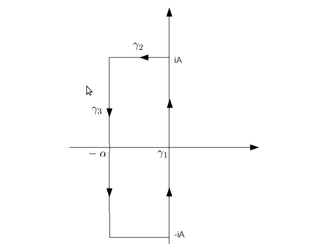
Figure 1: The closed path $\gamma_{1}\cup\gamma_{2}\cup\gamma_{3}\cup\gamma_{4}$ of Lemma 2.5.

In addition,

$$\begin{split}\left|\int_{\gamma_{2}}f(x,z)\,\text{d}z\right|&\leq\int_{0}^{\alpha}\left|\frac{\text{{e}}^{(-t+iA)x}}{(-t+iA-a)(-t+iA-b)}\right|\,\text{d}t\\ &=\int_{0}^{\alpha}\frac{\text{{e}}^{-tx}\text{d}t}{\sqrt{(t+\text{Re}\,a)^{2}+(A-\text{Im}\,a)^{2}}\sqrt{(t+\text{Re}\,b)^{2}+(A-\text{Im}\,b)^{2}}}\\ &\leq\frac{\alpha}{\sqrt{(\text{Re}\,a)^{2}+(A-\text{Im}\,a)^{2}}\sqrt{(\text{Re}\,b)^{2}+(A-\text{Im}\,b)^{2}}}\stackrel{{\scriptstyle A\rightarrow+\infty}}{{\longrightarrow}}0.\end{split}$$

The same argument leads to

$$\left|\int_{\gamma_{4}}f(z)\,\text{d}z\right|=\left|\int_{-\alpha}^{0}\frac{\text{{e}}^{(t-iA)x}}{(t-iA-a)(t-iA-b)}\,\text{d}t\right|\stackrel{{\scriptstyle A\rightarrow+\infty}}{{\longrightarrow}}0.$$

On the other hand,

$$\begin{split}\Big{|}\int_{\gamma_{3}}f(z)\,\text{d}z\Big{|}&\leq\text{{e}}^{-\alpha x}\int_{-A}^{A}\frac{\text{d}\theta}{|\alpha+i\theta+a||\alpha+i\theta+b|}\\ &\leq\text{{e}}^{-\alpha x}\int_{-\infty}^{+\infty}\frac{\text{d}\theta}{\sqrt{(\alpha+\text{Re}\,a)^{2}+(\theta-\text{Im}\,a)^{2}}\sqrt{(\alpha-\text{Re}\,b)^{2}+(\theta-\text{Im}\,b)^{2}}}\stackrel{{\scriptstyle\alpha\rightarrow+\infty}}{{\longrightarrow}}0.\end{split}$$

Then $\displaystyle\lim_{A\rightarrow+\infty}\int_{\gamma_{1}}f(x,z)\,\text{d}z=\int_{-\infty}^{+\infty}\frac{\text{{e}}^{i\theta x}}{(i\theta-a)(i\theta-b)}\,\text{d}\theta=0.$ ∎

Proof of Lemma 2.6.

For $z\in\mathbb{C}$ and $x\in\mathbb{R}$, set $g(x,z):=\frac{\text{{e}}^{xz}}{z}$. For any fixed $x>0$, one gets

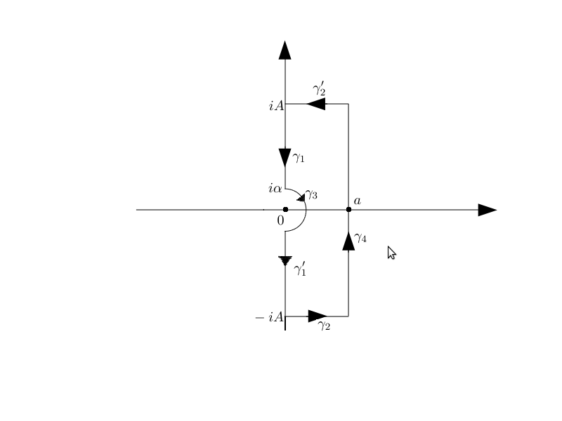
Figure 2: The closed path $\gamma_{1}\cup\gamma^{\prime}_{1}\cup\gamma_{2}\cup\gamma^{\prime}_{2}\cup\gamma_{3}\cup\gamma_{4}$ of Lemma 2.6.

$$\int_{\gamma_{1}\cup\gamma^{\prime}_{1}\cup\gamma_{2}\cup\gamma^{\prime}_{2}\cup\gamma_{3}\cup\gamma_{4}}g(x,z)\text{d}z=0,$$ (46)

where $\gamma_{k}$, $1\leq k\leq 6$, are the paths defined as follows (see Figure 2): for $A>\alpha>0$

• $\gamma_{1}$ is the oriented segment from $iA$ to $i\alpha$

• $\gamma^{\prime}_{1}$ is the oriented segment from $-i\alpha$ to $-iA$

• $\gamma_{2}$ is the oriented segment from $-iA$ to $a-iA$

• $\gamma^{\prime}_{2}$ is the oriented segment from $a+iA$ to $iA$

• $\gamma_{3}$ is the clockwise oriented arc of circle from $i\alpha$ to $-i\alpha$

• $\gamma_{4}$ is the oriented segment from $a-iA$ to $a+iA$

One gets

1. $\displaystyle\int_{\gamma_{1}\cup\gamma^{\prime}_{1}}g(x,z)\text{d}z=-2i\int_{\alpha}^{A}{\sin tx\over t}\text{d}t\stackrel{{\scriptstyle\begin{array}[]{c}\alpha\to 0\\ A\to+\infty\end{array}}}{{\longrightarrow}}-i\pi\ {\rm sgn}(x),$

2. $\displaystyle\Big{|}\int_{\gamma_{2}\cup\gamma^{\prime}_{2}}g(x,z)\text{d}z\Big{|}\leq 2{e^{ax}\over A}\stackrel{{\scriptstyle A\to+\infty}}{{\longrightarrow}}0,$

3. $\displaystyle\int_{\gamma_{3}}g(x,z)\text{d}z=-i\int_{-{\pi\over 2}}^{\pi\over 2}e^{x\alpha e^{i\theta}}\text{d}\theta\stackrel{{\scriptstyle\alpha\to 0}}{{\longrightarrow}}-i\pi$

and equality (46) thus implies

$$\int_{\gamma_{4}}g(x,z)\text{d}z=ie^{ax}\int_{-A}^{A}{e^{ix\theta}\over a+i\theta}\text{d}\theta\quad\stackrel{{\scriptstyle A\to+\infty}}{{\longrightarrow}}\quad i\pi(1+{\rm sgn}(x))$$

and the Lemma follows. ∎

3 On the factorization of $I-zP(\lambda)$

3.1 Preliminaries and motivation

We first introduce the two following stopping times, which correspond to the first entrance time of the random walk $(S_{n})_{n\geq 1}$ inside one of the semi-group $\mathbb{R}^{+},\mathbb{R}^{*+},\mathbb{R}^{-}$ and $\mathbb{R}^{*-}$ :

$$T_{+}=\inf\{n\geq 1,\,S_{n}\geq 0\};\qquad T^{*}_{+}=\inf\{n\geq 1,\,S_{n}>0\};$$

$$T_{-}=\inf\{n\geq 1,\,S_{n}\leq 0\};\qquad T^{*}_{-}=\inf\{n\geq 1,\,S_{n}<0\}.$$

Recall that $V_{N}[-\alpha_{0},\alpha_{0}]$ is the algebra of $N\times N$ matrices whose terms are Laplace transforms of Radon measures $\sigma$ on $\mathbb{R}$, satisfying $\displaystyle\int_{\mathbb{R}}\text{{e}}^{\lambda x}\text{d}|\sigma|(x)<+\infty$, for $|\text{Re}\ \lambda|\leq\alpha_{0}$. Let $G\in V_{N}[-\alpha_{0},\alpha_{0}]$, defined by

$$G(\lambda)=\left(\int_{\mathbb{R}}\text{{e}}^{\lambda x}\text{d}\sigma_{i,j}(x)\right)_{1\leq i,j\leq N}.$$

For $|\text{Re}\ \lambda|\leq\alpha_{0}$, we set ⁽⁾

$$\mathcal{N}G(\lambda)=\Big{(}\int_{]-\infty,0]}\text{{e}}^{\lambda x}\text{d}\sigma_{i,j}(x)\Big{)}_{i,j},\quad\mathcal{N}^{*}G(\lambda)=\Big{(}\int_{]-\infty,0[}\text{{e}}^{\lambda x}\text{d}\sigma_{i,j}(x)\Big{)}_{i,j};$$

$$\mathcal{P}G(\lambda)=\Big{(}\int_{[0,+\infty[}\text{{e}}^{\lambda x}\text{d}\sigma_{i,j}(x)\Big{)}_{i,j},\quad\mathcal{P}^{*}G(\lambda)=\Big{(}\int_{]0,+\infty[}\text{{e}}^{\lambda x}\text{d}\sigma_{i,j}(x)\Big{)}_{i,j}.$$

For $|z|<1$, we consider the following matrices of measures on $\mathbb{R}$:

$$B_{z}(\text{d}y)=\left(\sum_{n=1}^{+\infty}z^{n}\mathbb{P}_{i}\{S_{1}\geq S_{n},S_{2}\geq S_{n},\cdots,S_{n-1}\geq S_{n},S_{n}\in\text{d}y,X_{n}=j\}\right)_{i,j},$$

$$B^{*}_{z}(\text{d}y)=\left(\sum_{n=1}^{+\infty}z^{n}\mathbb{P}_{i}\{S_{1}>S_{n},S_{2}>S_{n},\cdots,S_{n-1}>S_{n},S_{n}\in\text{d}y,X_{n}=j\}\right)_{i,j},$$

$$C_{z}(\text{d}y)=\left(\sum_{n=1}^{+\infty}z^{n}\mathbb{P}_{i}\{S_{1}\geq 0,S_{2}\geq 0,\cdots,S_{n-1}\geq 0,S_{n}\in\text{d}y,X_{n}=j\}\right)_{i,j},$$

$$C^{*}_{z}(\text{d}y)=\left(\sum_{n=1}^{+\infty}z^{n}\mathbb{P}_{i}\{S_{1}>0,S_{2}>0,\cdots,S_{n-1}>0,S_{n}\in\text{d}y,X_{n}=j\}\right)_{i,j}.$$

For $\text{Re}\ \lambda=0$, the related Laplace transforms of the above measures, denoted respectively by $B_{z}(\lambda)$, $B^{*}_{z}(\lambda)$, $C_{z}(\lambda)$ and $C^{*}_{z}(\lambda)$, are defined as following:

$$B_{z}(\lambda)=\int_{-\infty}^{+\infty}\text{{e}}^{\lambda y}B_{z}(\text{d}y),\quad B^{*}_{z}(\lambda)=\int_{-\infty}^{+\infty}\text{{e}}^{\lambda y}B^{*}_{z}(\text{d}y);$$

$$C_{z}(\lambda)=\int_{-\infty}^{+\infty}\text{{e}}^{\lambda y}C_{z}(\text{d}y),\quad C^{*}_{z}(\lambda)=\int_{-\infty}^{+\infty}\text{{e}}^{\lambda y}C^{*}_{z}(\text{d}y).$$

Note that the series which appear in these formulas do converge for $|z|<1$ and that the matrices$B_{z}(\lambda)$, $B^{*}_{z}(\lambda)$, $C_{z}(\lambda)$ and $C^{*}_{z}(\lambda)$ belong to $V_{N}[0,0]$.

Let us now explain briefly how we will use these waiting times to prove the local limit theorem for the process $m_{n}:=\min(0,S_{1},\cdots,S_{n})$. Indeed, the Laplace transform of $m_{n}$ may be expressed in terms of the operators $\mathcal{N}^{*}$ and $\mathcal{P}$ and the matrices $B^{*}_{z}$ and $C_{z}$ ; we have the

Lemma 3.1.

For $\lambda>0$ and $|z|<1$,

$$\sum_{n=0}^{+\infty}z^{n}\mathbb{E}_{i}(\text{{e}}^{\lambda m_{n}};X_{n}=j)=\{[I+\mathcal{N}^{*}B^{*}_{z}(\lambda)][I+\mathcal{P}C_{z}(0)]\}_{i,j}.$$ (47)

Proof.

Applying Markov property to the process $(X_{n},S_{n})$, we get

$$\begin{split}&\sum_{n=0}^{+\infty}z^{n}\mathbb{E}_{i}(\text{{e}}^{\lambda m_{n}};X_{n}=j)\\ =&\sum_{n=0}^{+\infty}z^{n}\sum_{k=0}^{n}\mathbb{E}_{i}(\text{{e}}^{\lambda S_{k}};S_{0}>S_{k},\cdots,S_{k-1}>S_{k},S_{k+1}\geq S_{k},\cdots,S_{n}\geq S_{k},X_{n}=j)\\ =&\sum_{n=0}^{+\infty}z^{n}\sum_{k=0}^{n}\sum_{l\in E}\mathbb{E}_{i}(\text{{e}}^{\lambda S_{k}};S_{1}>S_{k},\cdots,S_{k-1}>S_{k},S_{k}<0,X_{k}=l)\;\mathbb{E}_{l}(S_{1}\geq 0,\cdots,S_{n-k}\geq 0,X_{n-k}=j)\\ =&\sum_{l\in E}\left[\sum_{k=0}^{+\infty}z^{k}\mathbb{E}_{i}(\text{{e}}^{\lambda S_{k}};S_{1}>S_{k},\cdots,S_{k-1}>S_{k},S_{k}<0,X_{k}=l)\right]\left[\sum_{p=0}^{+\infty}z^{p}\mathbb{E}_{l}(S_{1}\geq 0,\cdots,S_{p}\geq 0,X_{p}=j)\right]\\ =&\Big{\{}[I+\mathcal{N}^{*}B^{*}_{z}(\lambda)][I+\mathcal{P}C_{z}(0)]\Big{\}}_{i,j}.\end{split}$$

∎

We will have to study the regularity with respect to $z$ and $\lambda$ of each factor $I+\mathcal{N}^{*}B^{*}_{z}(\lambda)$ and $I+\mathcal{P}C_{z}(0)$ ; to do this, we will use a classical approach based on the so-called Wiener-Hopf factorization.

3.2 The initial probabilistic factorization

We have the

Proposition 3.1.

For $\text{Re}\ \lambda=0$ and $|z|<1$, one gets

$$I-zP(\lambda)=(I-\mathcal{P}B^{*}_{z}(\lambda))(I-\mathcal{N}^{*}C_{z}(\lambda)),$$ (48)

$$(I-\mathcal{P}B^{*}_{z}(\lambda))^{-1}=I+\mathcal{P}C_{z}(\lambda),$$ (49)

$$(I-\mathcal{N}^{*}C_{z}(\lambda))^{-1}=I+\mathcal{N}^{*}B^{*}_{z}(\lambda).$$ (50)

Proof.

We first check that

$$(I-\mathcal{N}^{*}C_{z}(\lambda))(I-zP(\lambda))^{-1}=I+\mathcal{P}C_{z}(\lambda),$$ (51)

and (48) will follow by (49). Note that, for $\text{Re}\ \lambda=0$, $r(P(\lambda))\leq r(P(0))=1$. So for $|z|<1$, $(I-zP(\lambda))$ is invertible, with inverse

$$(I-zP(\lambda))^{-1}=I+\sum_{n=1}^{+\infty}z^{n}P^{n}(\lambda).$$

By the definition of $P(\lambda)$ and the strong Markov property, we get

$$\begin{split}&\delta_{i,j}+\sum_{n=1}^{+\infty}z^{n}(P^{n}(\lambda))_{i,j}\\ &=\delta_{i,j}+\sum_{n=1}^{+\infty}\mathbb{E}_{i}(z^{n}\text{{e}}^{\lambda S_{n}};X_{n}=j)\\ &=\delta_{i,j}+\mathbb{E}_{i}\left(\sum_{n=1}^{T^{*}_{-}-1}z^{n}\text{{e}}^{\lambda S_{n}};X_{n}=j\right)+\mathbb{E}_{i}\left(\sum_{n=T^{*}_{-}}^{+\infty}z^{n}\text{{e}}^{\lambda S_{n}};X_{n}=j\right)\\ &=\delta_{i,j}+\mathbb{E}_{i}\left(\sum_{n=1}^{+\infty}z^{n}\text{{e}}^{\lambda S_{n}};T^{*}_{-}\geq n+1;X_{n}=j\right)+\mathbb{E}_{i}\left\{z^{T^{*}_{-}}\text{{e}}^{\lambda S_{T^{*}_{-}}}\left[\mathbb{E}_{X_{T^{*}_{-}}}\left(\sum_{n=0}^{+\infty}z^{n}\text{{e}}^{\lambda S_{n}};X_{n}=j\right)\right]\right\}\\ &=\delta_{i,j}+(\mathcal{P}C_{z}(\lambda))_{i,j}+\sum_{l\in E}\left\{\left[\mathbb{E}_{i}\left(\sum_{k=1}^{+\infty}z^{k}\text{{e}}^{\lambda S_{k}};T^{*}_{-}=k;X_{k}=l\right)\right]\left[\sum_{n=0}^{+\infty}\mathbb{E}_{l}\left(z^{n}\text{{e}}^{\lambda S_{n}};X_{n}=j\right)\right]\right\}\\ &=\delta_{i,j}+(\mathcal{P}C_{z}(\lambda))_{i,j}\\ &\qquad+\sum_{l\in E}\left\{\left[\sum_{k=1}^{+\infty}z^{k}\mathbb{E}_{i}(\text{{e}}^{\lambda S_{k}};S_{1}\geq 0,S_{2}\geq 0,\cdots,S_{k-1}\geq 0,S_{k}<0;X_{k}=l)\right]\left[\delta_{l,j}+\sum_{n=1}^{+\infty}\mathbb{E}_{l}(z^{n}\text{{e}}^{\lambda S_{n}};X_{n}=j)\right]\right\}\\ &=\delta_{i,j}+(\mathcal{P}C_{z}(\lambda))_{i,j}+\sum_{l\in E}\left(\mathcal{N}^{*}C_{z}(\lambda)\right)_{i,l}((I-zP(\lambda))^{-1})_{l,j}\\ &=\delta_{i,j}+(\mathcal{P}C_{z}(\lambda))_{i,j}+\left(\mathcal{N}^{*}C_{z}(\lambda)(I-zP(\lambda))^{-1}\right)_{i,j}.\end{split}$$

We now prove (49) (and the proof of (48) will be complete, as we claimed above). Set $F_{z}(\lambda)=(I-\mathcal{P}B^{*}_{z}(\lambda))(I+\mathcal{P}C_{z}(\lambda))$ ; we want to check that $F_{z}(\lambda)=I$. One gets

$$\Big{(}F_{z}(\lambda)\Big{)}_{i,j}=\delta_{i,j}+\Big{(}\mathcal{P}C_{z}(\lambda)\Big{)}_{i,j}-\Big{(}\mathcal{P}B^{*}_{z}(\lambda)\Big{)}_{i,j}-\Big{(}\mathcal{P}B^{*}_{z}(\lambda)\mathcal{P}C_{z}(\lambda)\Big{)}_{i,j}.$$ (52)

By the strong Markov property, we get

$$\begin{split}&\Big{(}\mathcal{P}B^{*}_{z}(\lambda)\mathcal{P}C_{z}(\lambda)\Big{)}_{i,j}\\ =&\sum_{n=1}^{+\infty}z^{n}\mathbb{E}_{i}\left[\text{{e}}^{\lambda S_{n}};S_{1}>S_{n},S_{2}>S_{n},\cdots,S_{n-1}>S_{n}\geq 0;\mathbb{E}_{X_{n}}\left(\sum_{k=1}^{+\infty}z^{k}\text{{e}}^{\lambda S_{k}};S_{1}\geq 0,\cdots,S_{k}\geq 0,X_{k}=j\right)\right]\\ =&\sum_{n\geq 1,k\geq 1}z^{n+k}\mathbb{E}_{i}[\text{{e}}^{\lambda S_{n+k}};S_{1}>S_{n},\cdots,S_{n-1}>S_{n},S_{n+1}\geq S_{n},\cdots,S_{n+k}\geq S_{n}\geq 0,X_{n+k}=j]\\ =&\sum_{m=2}^{+\infty}z^{m}\left[\sum_{n=1}^{m-1}\mathbb{E}_{i}(\text{{e}}^{\lambda S_{m}};S_{1}>S_{n},\cdots,S_{n-1}>S_{n},S_{n+1}\geq S_{n},\cdots,S_{m}\geq S_{n}\geq 0,X_{m}=j)\right].\end{split}$$ (53)

Therefore,

$$\begin{split}(F_{z}(\lambda))_{i,j}=\ &\delta_{i,j}+\sum_{m=1}^{+\infty}z^{m}\mathbb{E}_{i}(\text{{e}}^{\lambda S_{m}};S_{1}\geq 0,S_{2}\geq 0,\cdots,S_{m}\geq 0,X_{m}=j)\\ &-\sum_{m=1}^{+\infty}z^{m}\mathbb{E}_{i}(\text{{e}}^{\lambda S_{m}};S_{1}>S_{m},S_{2}>S_{m},\cdots,S_{m-1}>S_{m}\geq 0;X_{m}=j)\\ &-\sum_{m=2}^{+\infty}z^{m}\left[\sum_{n=1}^{m-1}\mathbb{E}_{i}(\text{{e}}^{\lambda S_{m}};S_{1}>S_{n},\cdots,S_{n-1}>S_{n},S_{n+1}\geq S_{n},\cdots,S_{m}\geq S_{n}\geq 0,X_{m}=j)\right]\\ =\ &\delta_{i,j}+\sum_{m=1}^{+\infty}z^{m}\mathbb{E}_{i}(\text{{e}}^{\lambda S_{m}};S_{1}\geq 0,S_{2}\geq 0,\cdots,S_{m}\geq 0,X_{m}=j)-z\mathbb{E}_{i}(\text{{e}}^{\lambda S_{1}};S_{1}\geq 0,X_{1}=j)\\ &-\sum_{m=2}^{+\infty}z^{m}\left[\sum_{n=1}^{m}\mathbb{E}_{i}(\text{{e}}^{\lambda S_{m}};S_{1}>S_{n},\cdots,S_{n-1}>S_{n},S_{n+1}\geq S_{n},\cdots,S_{m}\geq S_{n}\geq 0,X_{m}=j)\right]\\ =\ &\delta_{i,j}+\sum_{m=1}^{+\infty}z^{m}\mathbb{E}_{i}(\text{{e}}^{\lambda S_{m}};S_{1}\geq 0,S_{2}\geq 0,\cdots,S_{m}\geq 0,X_{m}=j)\\ &-\sum_{m=1}^{+\infty}z^{m}\left[\sum_{n=1}^{m}\mathbb{E}_{i}(\text{{e}}^{\lambda S_{m}};S_{1}>S_{n},\cdots,S_{n-1}>S_{n},S_{n+1}\geq S_{n},\cdots,S_{m}\geq S_{n}\geq 0,X_{m}=j)\right]\end{split}$$

To prove $F_{z}(\lambda)=I$, we have to check that, for any $m\geq 1$,

$$\begin{split}&\mathbb{E}_{i}(\text{{e}}^{\lambda S_{m}};S_{1}\geq 0,S_{2}\geq 0,\cdots,S_{m}\geq 0,X_{m}=j)\\ &\qquad\qquad\qquad=\sum_{n=1}^{m}\mathbb{E}_{i}(\text{{e}}^{\lambda S_{m}};S_{1}>S_{n},\cdots,S_{n-1}>S_{n},S_{n}\geq 0,S_{n+1}\geq S_{n},\cdots,S_{m}\geq S_{n},X_{m}=j).\end{split}$$

Let us thus consider the random variables $T_{m},m\geq 1,$ defined by

$$T_{m}=\inf\{1\leq n\leq m:S_{n}=\inf(S_{1},\cdots,S_{m})\}.$$

We have the following equalities

$$\begin{split}&\mathbb{E}_{i}(\text{{e}}^{\lambda S_{m}};S_{1}\geq 0,S_{2}\geq 0,\cdots,S_{m}\geq 0,X_{m}=j)\\ =&\sum_{n=1}^{m}\mathbb{E}_{i}(\text{{e}}^{\lambda S_{m}};S_{1}\geq 0,S_{2}\geq 0,\cdots,S_{m}\geq 0,T_{m}=n,X_{m}=j)\\ =&\sum_{n=1}^{m}\mathbb{E}_{i}(\text{{e}}^{\lambda S_{m}};S_{1}>S_{n},\cdots,S_{n-1}>S_{n},S_{n}\geq 0,S_{n+1}\geq S_{n},\cdots,S_{m}\geq S_{n},X_{m}=j),\end{split}$$

which achieves the proof.

The proof of the equality (50) goes along the same lines. ∎

Remarks 3.1.

1)

When $E$ reduces to one point, the sequence $(S_{n})_{n\geq 0}$ is a random walk on $\mathbb{R}$ and Proposition 3.1 corresponds to the classical Wiener-Hopf factorization ([5]).

2)

There is another way to express the matrices $\mathcal{N}^{*}C_{z}(\lambda)$ and $\mathcal{P}B^{*}_{z}(\lambda)$ ; for $|z|<1$, one gets

$$\mathcal{N}^{*}C_{z}(\lambda)=\Big{\{}\mathbb{E}_{i}\Big{(}z^{T_{-}^{*}}\text{{e}}^{\lambda S_{T_{-}^{*}}};X_{T_{-}^{*}}=j\Big{)}\Big{\}}_{i,j}\quad{\rm when}\quad\text{Re}\ \lambda\geq 0$$

$$\mathcal{P}B^{*}_{z}(\lambda)=X^{-1}\Big{\{}\mathbb{E}_{i}\Big{(}z^{\widetilde{T}_{+}^{*}}\text{{e}}^{\lambda\widetilde{S}_{\widetilde{T}_{+}^{*}}};X_{\widetilde{T}_{+}^{*}}=j\Big{)}\Big{\}}_{i,j}^{\Large t}X\quad{\rm when}\quad\text{Re}\ \lambda\leq 0\quad^{(}^{)}$$

where $X$ is the diagonal matrice $\displaystyle X:=\begin{pmatrix}\nu_{1}&\quad&(0)\\ \quad&\ddots&\quad\\ (0)&\quad&\nu_{N}\end{pmatrix}.$

To explain (briefly) how two obtain for instance this “new” expression of $\mathcal{N}^{*}C_{z}(\lambda)$, we introduce the dual chain $(\widetilde{S}_{n},\widetilde{X}_{n})$ of $(S_{n},X_{n})$ whose transition probability is given by

$$\widetilde{P}_{(i,x)}(\{j\}\times A)=\frac{\nu_{j}}{\nu_{i}}p_{j,i}F(A-x,j,i).$$

We also consider the $N\times N$ matrice $\widetilde{C}^{-}_{z}$ defined by :

for $|z|<1$, $|\text{Re}\ \lambda|\leq\alpha_{0}$

$$\widetilde{C}^{-}_{z}=\left(\sum_{n=1}^{+\infty}z^{n}\mathbb{E}_{i}(\text{{e}}^{\lambda\widetilde{S}_{n}},\widetilde{S}_{1}\leq 0,\widetilde{S}_{2}\leq 0,\cdots,\widetilde{S}_{n-1}\leq 0,\widetilde{X}_{n}=j)\right)_{i,j}.$$

The remark (2) is a straightforward consequence of the

Fact 3.1.

One gets $\widetilde{C}_{z}^{-}=X^{-1}(B^{*}_{z})^{t}X.$

Proof.

We have the equality

$$\begin{split}&\mathbb{E}_{i}(\text{{e}}^{\lambda\widetilde{S}_{n}},\,\widetilde{S}_{1}\leq 0,\,\cdots,\widetilde{S}_{n-1}\leq 0,\,\widetilde{X}_{n}=j)\\ =&\sum_{k_{1},\,k_{2},\cdots,k_{n-1}}\int_{\mathbb{R}^{n}}\frac{\nu_{k_{1}}}{\nu_{i}}\,\frac{\nu_{k_{2}}}{\nu_{k_{1}}}\cdots\frac{\nu_{j}}{\nu_{k_{n-1}}}\,\text{{e}}^{\lambda(\widetilde{y}_{1}+\cdots\widetilde{y}_{n})}1_{[\widetilde{y}_{1}\leq 0]}\,1_{[\widetilde{y}_{1}+\widetilde{y}_{2}\leq 0]}\cdots 1_{[\widetilde{y}_{1}+\cdots+\widetilde{y}_{n}\leq 0]}\\ &\qquad\times F(k_{1},i,\text{d}\widetilde{y}_{1})P_{k_{1},i}F_{(}k_{2},k_{1},\text{d}\widetilde{y}_{2})P_{k_{2},k_{1}}\cdots F(j,k_{n-1},\text{d}\widetilde{y}_{n})P_{j,k_{n-1}}.\end{split}$$

Replacing in this equality $\widetilde{y}_{k}$ by $y_{n+1-k}$ and $\widetilde{X}_{k}$ by $X_{n-k}$ for all $0\leq k\leq n$, we obtain

$$\begin{split}&\mathbb{E}_{i}(\text{{e}}^{\lambda\widetilde{S}_{n}},\,\widetilde{S}_{1}\leq 0,\,\cdots,\widetilde{S}_{n-1}\leq 0,\,\widetilde{X}_{n}=j)\\ =&\frac{\nu_{j}}{\nu_{i}}\sum_{k_{1},\cdots,k_{n-1}}\mathbb{E}(\text{{e}}^{\lambda S_{n}},S_{n}\leq S_{n-1},\cdots,S_{n}\leq S_{1},X_{0}=j,X_{1}=k_{n-1},\cdots,X_{n-1}=k_{1},X_{n}=i)\\ =&\frac{\nu_{j}}{\nu_{i}}\;\mathbb{E}_{j}(\text{{e}}^{\lambda S_{n}},S_{1}\geq S_{n},S_{2}\geq S_{n},\cdots,S_{n-1}\geq S_{n},X_{n}=i).\end{split}$$

Therefore, $\widetilde{C}_{z}^{-}(\lambda)_{i,j}=\frac{\nu_{j}}{\nu_{i}}B^{*}_{z}(\lambda)_{j,i}.$ ∎

In the sequel, we will extend this factorization to a larger set of parameters. We will first prove, by arguments of elementary type, that this identity is valid for $|z|\leq 1$ and ${\rm Re}\ \lambda\in[-\alpha_{0},\alpha_{0}]$. In a second step, we will extend this identity for ${\rm Re}\ \lambda=0$ and $z$ in a neigbourhood of the unit disc, excepted the point $1$ ; this is much more delicate and it relies on a general argument of algebraic type, due to Presman ([13]).

3.3 General factorization theory of Presman

Let ${\mathfrak{R}}$ be an arbitrary algebraic ring with unit element $e$ and $\mathcal{I}$ be the identity operator in ${\mathfrak{R}}$. Let the additive operator $\mathfrak{N}$ be defined on a two-side ideal ${\mathfrak{R}}^{\prime}$ of the ring ${\mathfrak{R}}$, with

$$({\mathfrak{N}}f)({\mathfrak{N}}g)={\mathfrak{N}}[({\mathfrak{N}}f)g+f({\mathfrak{N}}g)-fg]$$ (54)

holding for any $f,g\in{\mathfrak{R}}^{\prime}$. It is easy to check that the operator $\mathfrak{P}=\mathcal{I}-{\mathfrak{N}}$ also satisfies the relation (54).

Definition 3.1.

We say that the element $e-a$ of a ring ${\mathfrak{R}}$ admits a left canonical factorization with respect to the operator ${\mathfrak{N}}$ (l.c.f. ${\mathfrak{N}}$) if $a\in{\mathfrak{R}}^{\prime}$ and if there exist $b,c\in{\mathfrak{R}}^{\prime}$ such that

$$e-a=(e-{\mathfrak{P}}b)(e-{\mathfrak{N}}c)$$ (55)

$$(e-{\mathfrak{P}}b)^{-1}=e+{\mathfrak{P}}c$$ (56)

$$(e-{\mathfrak{N}}c)^{-1}=e+{\mathfrak{N}}b.$$ (57)

In this case, we say that $b$ and $c$ provide a l.c.f. ${\mathfrak{N}}$. We call $e-{\mathfrak{P}}b$ and $e-{\mathfrak{N}}c$ respectively, the positive and negative components of the l.c.f. ${\mathfrak{N}}$.

The following lemma states the uniqueness of such a factorization once it exists.

Lemma 3.2 ([13], lemma 1.1).

1. If $b$ and $c$ provide a l.c.f ${\mathfrak{N}}$ of the element $e-a$ then

   1. the l.c.f. ${\mathfrak{N}}$ is unique and is determined by any one of the elements ${\mathfrak{N}}b$, ${\mathfrak{P}}b$, ${\mathfrak{N}}c$, ${\mathfrak{P}}c$;

   2. for any $\text{d}\in{\mathfrak{R}}$, the equations

      $$x-{\mathfrak{P}}(xa)=d,\quad y-{\mathfrak{N}}(ay)=d$$ (58)

      have a unique solution, given by the formulas:

      $$x=d+\{{\mathfrak{P}}[da(e+{\mathfrak{N}}b)]\}(e+{\mathfrak{P}}c),$$ (59)

      $$y=d+(e+{\mathfrak{N}}b){\mathfrak{N}}[(e+{\mathfrak{P}}c)ad];$$ (60)

   3. for $d=e$, the elements $x=e+{\mathfrak{P}}c$ and $y=e+{\mathfrak{N}}b$ are solutions of equation (58);

   4. $c_{1}=c$ (resp. $b_{1}=b$) is the unique solution of the equation

      $$(e+{\mathfrak{P}}C_{1})(e-a)=e-{\mathfrak{N}}C_{1}\quad(\text{ resp. }(e-a)(e+{\mathfrak{N}}b_{1})=e-{\mathfrak{P}}b).$$

2. If, for $d=e$, equations (58) have solutions $x^{\prime}$ and $y^{\prime}$, then $x^{\prime}(e-a)y^{\prime}=e$; moreover, if any two of the three elements $x^{\prime}$, $y^{\prime}$, $e-a$ are invertible, then $b^{\prime}=ay^{\prime}$ and $c^{\prime}=x^{\prime}a$ provide a l.c.f. ${\mathfrak{N}}$ of the element $e-a$.

Now, we assume that $a$ depends analytically on the complex variable $z$ in a neigbourhood of some $z_{0}$ and describe the regularity of the two components of the l.c.f $\mathfrak{N}$ ; namely, we get the following

Lemma 3.3 ([13], lemma 1.2).

Let $a(z)$ be an analytic function in a neighborhood of the point $z_{0}$, taking values in an ideal ${\mathfrak{R}}^{\prime}$ of the Banach algebra ${\mathfrak{R}}$ and suppose that $b_{0}$ and $c_{0}$ provide a l.c.f. ${\mathfrak{N}}$ of the element $e-a(z_{0})$. Then $e-a(z)$ admits l.c.f. ${\mathfrak{N}}$ in a neighborhood of the point $z_{0}$, where the elements $b(z)$ and $c(z)$ which provide the l.c.f. ${\mathfrak{N}}$ of the element $e-a(z)$ are analytic functions of $z$ taking values in ${\mathfrak{R}}^{\prime}$.

We achieve this paragraph explaining how one will use this general result in our context.

We will consider the algebraic ring $V_{N}[-\alpha_{0},\alpha_{0}]$ of $N\times N$ matrices whose terms are Laplace transforms of Radon measures $\sigma$ on $\mathbb{R}$, with exponential moment of order $\alpha_{0}$ The operator ${\mathfrak{N}}$ will be here the operator $\mathcal{N}^{*}$ defined above and acting on $V_{N}[-\alpha_{0},\alpha_{0}]$ and $\mathfrak{P}$ will be equal to $\mathcal{P}$.

If $\nu$, $\mu$ are two Radon measures on $\mathbb{R}$, we have the following identity :

$$\nu^{*-}\ast\mu^{*-}=(\nu^{*-}\ast\mu+\nu\ast\mu^{*-}-\nu\ast\mu)^{*-}.\quad^{(}^{)}$$

Taking into account this equality, we obtain that $\mathcal{N}^{*}$ and $\mathcal{P}$ both satisfy the identity (54) for any $f$, $g\in V_{N}[a,b]$.

For $|z|<1$ and $|\text{Re}\ \lambda|\leq\alpha_{0}$, we will consider the following $\mathbb{C}$-valued $N\times N$ matrices:

$$B^{*}_{z}(\lambda):=\left(\sum_{n=1}^{+\infty}z^{n}\int_{-\infty}^{+\infty}\text{{e}}^{\lambda y}\text{d}\mathbb{P}_{i}\{S_{1}>S_{n},S_{2}>S_{n},\cdots,S_{n-1}>S_{n},S_{n}\leq y,X_{n}=j\}\right)_{i,j},$$

$$C_{z}(\lambda):=\left(\sum_{n=1}^{+\infty}z^{n}\int_{-\infty}^{+\infty}\text{{e}}^{\lambda y}\text{d}\mathbb{P}_{i}\{S_{1}\geq 0,S_{2}\geq 0,\cdots,S_{n-1}\geq 0,S_{n}\leq y,X_{n}=j\}\right)_{i,j}.$$

Recall now that $P(\lambda)$ belongs to $V_{N}[-\alpha_{0},\alpha_{0}]$ ; furthermore, by Proposition 3.1, for any complex number $z$ with modulus $<1$ and any $\lambda\in\mathbb{C}$ such that Re$\ \lambda=0$, the operator $I-zP(\lambda)$ admits a l.c.f $\mathcal{N}^{*}$ on $V_{N}[0,0]$ provided with $B^{*}_{z}$ and $C_{z}$.

The above general Presman’s result are therefore applicable to $z\mapsto A_{z}:=zP(\lambda)$ with values in $V_{N}[-\alpha_{0},\alpha_{0}]$ for $|z|<1$ and analytic on the unit open disc of the complex plane.

In particular, the elements $B^{*}_{z}$ and $C_{z}$ belong to $V_{N}[0,0]$. In fact, one may precise this last statement, with the following lemma due to Presman (Lemma 1.3 in [13]) :

Lemma 3.4.

If $I-A_{z}$ is an analytic function of $z$ in a neighbourhood of the point $z_{0}$, taking values in the ring $V_{N}[-\alpha_{0},\alpha_{0}]$ and if in this neighbourhood $I-A_{z}$, as an element of $V_{N}[0,0]$, admits a l.c.f. with respect to $\mathcal{N}^{*}$ with corresponding elements $B^{*}_{z}$ and $C_{z}$, then $\mathcal{P}B^{*}_{z}$ (resp. $\mathcal{N}^{*}C_{z}$) is analytic in $z$ in this neigbourhood, with values in $\mathcal{P}V_{N}]-\infty,\alpha_{0}]$ (resp. $\mathcal{N}^{*}V_{N}[-\alpha_{0},+\infty[$).

In the sequel, we analyze the factorization of $I-zP(\lambda)$ in a neigbourhood of the unit disc of the complex plane for some values of $\lambda\in\mathbb{C}$ ; we thus introduce the

Notation 3.1.

We will denote by $\mathbb{D}$ the closed unit ball in the complex number plane :

$$\mathbb{D}:=\{z\in\mathbb{C}:|z|\leq 1\}.$$

The open unit ball will be denoted $\mathbb{D}^{\circ}$.

3.4 The factorization of $I-zP(\lambda)$ for $z\in\mathbb{D}^{\circ}$ and $\text{Re}\ \lambda$ closed to $0$

We first state the the following

Theorem 3.1.

There exists $\alpha_{1}\in]0,\alpha_{0}[$ such that for any $z\in\mathbb{D}^{\circ}$, one gets

1. For $-\alpha_{1}\leq\text{Re}\ \lambda\leq\alpha_{1}$,

   $$I-zP(\lambda)=(I-\mathcal{P}B^{*}_{z}(\lambda))(I-\mathcal{N}^{*}C_{z}(\lambda)),$$ (61)

2. For $\text{Re}\ \lambda\leq 0$,

   $$(I-\mathcal{P}B^{*}_{z}(\lambda))^{-1}=I+\mathcal{P}C_{z}(\lambda),$$ (62)

3. For $\text{Re}\ \lambda\geq 0$,

   $$(I-\mathcal{N}^{*}C_{z}(\lambda))^{-1}=I+\mathcal{N}^{*}B^{*}_{z}(\lambda).$$ (63)

Furthermore, the maps $z\mapsto\mathcal{P}B^{*}_{z}(\lambda)$ and $z\mapsto\mathcal{N}^{*}C_{z}(\lambda)$ are analytic on $\mathbb{D}^{\circ}$ with values $\mathcal{P}V_{N}]-\infty,\alpha_{1}]$ (resp. $\mathcal{N}^{*}V_{N}[-\alpha_{1},+\infty[$).

Proof.

By the argument developped to establish Proposition 3.1, one checks easily that (49) (resp. (50)) is valid for $|z|<1$ and ${\rm Re}\ \lambda\leq 0$ ( resp. ${\rm Re}\ \lambda\geq 0$). So (62) and (63) are valid.

The existence of the factorization in $V_{N}[0,0]$ for any $z\in\mathbb{D}^{\circ}$ is given by Proposition 3.1. The analyticity of the different components $B^{*}_{z}(\lambda)$ and $C_{z}(\lambda)$ on $\mathbb{D}^{\circ}$ for $\text{Re}\ \lambda=0$ is a consequence of Lemma 3.3 ; we may also apply Lemma 3.4 and conclude that

$$\mathcal{P}B^{*}_{z}\in\mathcal{P}V_{N}]-\infty,\alpha_{0}]\quad\mbox{\rm and}\quad\mathcal{N}^{*}C_{z}\in\mathcal{N}^{*}V_{N}[-\alpha_{0},+\infty[.$$

Now, for any $z\in\mathbb{D}^{\circ}$, the maps $\lambda\mapsto I-zP(\lambda)$ and $\lambda\mapsto(I-\mathcal{P}B^{*}_{z}(\lambda))(I-\mathcal{N}^{*}C_{z}(\lambda))$ are analytic on the strip $\{|{\rm Re}\ \lambda|\leq\alpha_{1}\}$ for any $\alpha_{1}\in]0,\alpha_{0}[$ and they coincide on the line ${\rm Re}\ \lambda=0$ ; they thus coincide as analytic functions on the strip $\{|{\rm Re}\ \lambda|\leq\alpha_{1}\}$. So (61) holds for $-\alpha_{1}\leq\text{Re}\ \lambda\leq\alpha_{1}$ ; the analyticity of the maps $z\mapsto\mathcal{P}B^{*}_{z}(\lambda)$ and $z\mapsto\mathcal{N}^{*}C_{z}(\lambda)$ are analytic on $\mathbb{D}^{\circ}$ with values $\mathcal{P}V_{N}]-\infty,\alpha_{1}]$ (resp. $\mathcal{N}^{*}V_{N}[-\alpha_{1},+\infty[$ ) is a direct consequence of Lemma 3.4.

For the analyticity of these two maps when $\text{Re}\ \lambda\in]-\alpha_{1},\alpha_{1}]$, one may also use the explicit form of the functions $B^{*}_{z}$ and $C_{z}$ and argue as follows :
- for $\text{Re}\ \lambda=0$, it is a consequence of Lemma 3.3 as we said a few lines above ;
- when $\text{Re}\ \lambda>0$, it is a direct consequence of the identity

$$\mathcal{N}^{*}C_{z}(\lambda)=\Big{\{}\mathbb{E}_{i}\Big{(}z^{T_{-}^{*}}\text{{e}}^{\lambda S_{T_{-}^{*}}};X_{T_{-}^{*}}=j\Big{)}\Big{\}}_{i,j};$$

- when $\text{Re}\ \lambda\in[-\alpha_{1},0[$, we use (61) and (62) to write

$$\mathcal{N}^{*}C_{z}(\lambda)=I-(I+\mathcal{P}C_{z}(\lambda))(I-zP(\lambda))$$

with $\displaystyle\mathcal{P}C_{z}(\lambda)=\Big{\{}\sum_{n\geq 0}z^{n}\mathbb{E}_{i}\Big{(}\text{{e}}^{\lambda S_{n}};T_{-}^{*}>n,X_{n}=j\Big{)}\Big{\}}_{i,j}.$ The two factors on the right hand side of this last equality are clearly analytic in $z\in\mathbb{D}^{\circ}$ and the result follows. The same argument holds for $z\mapsto\mathcal{P}B^{*}_{z}(\lambda)$. ∎

3.5 Expansion of the factorization outside the unit disc and far from $z=1$

We study here the extension of the preceding factorization when $\text{Re}\ \lambda\ =0$ and $z$ lives in a neighbourhood of $\mathbb{D}\setminus\{1\}$. We have the

Theorem 3.2.

There exists a neighbourhood $U$ of $\mathbb{D}\setminus\{1\}$ such that, for $\text{Re}\ \lambda=0$, the two maps $z\mapsto B^{*}_{z}(\lambda)$ and $z\mapsto C_{z}(\lambda)$ may be continuously expanded on $U$ in such a way

1. for any $z\in U$, the formulas (61), (62) and (63) hold.

2. the maps $z\mapsto\mathcal{P}B^{*}_{z}$ and $z\mapsto\mathcal{N}^{*}C_{z}$ are analytic on $U$, with values in $V_{N}]-\infty,\alpha_{0}]$ and $V_{N}[-\alpha_{0},+\infty[$ respectively.

Proof.

We fix $\lambda$ s.t. $\text{Re}\ \lambda=0$, $z_{0}\in\mathbb{C}$ with $|z_{0}|=1,z_{0}\neq 1$ and choose a sequence $(z_{n})_{n\geq 1}$ of complex numbers in $\mathbb{D}^{\circ}$ which converges to $z_{0}$.

By 2) of Remarks 3.1, the two limits $\displaystyle B^{+}_{z_{0}}(\lambda):=\lim_{n\to+\infty}\mathcal{P}B^{*}_{z_{n}}(\lambda)$ and $\displaystyle C^{*-}_{z_{0}}(\lambda):=\lim_{n\to+\infty}\mathcal{N}^{*}C_{z_{n}}(\lambda)$ do exist ; furthermore, (61) holds at any point $z_{n}$ and letting $n\to+\infty$ one gets

$$I-z_{0}P(\lambda)=(I-B^{+}_{z_{0}}(\lambda))(I-C^{*-}_{z_{0}}(\lambda)).$$

Since $z_{0}\neq 1$, the matrice $I-z_{0}P(\lambda)$ is invertible, so is $I-B^{+}_{z_{0}}(\lambda)$ ; by (62), the limit $\displaystyle\lim_{n\to+\infty}PC_{z_{n}}(\lambda)$ does also exists (and is equal to $C_{z_{0}}^{+}(\lambda):=-I+(I-B^{+}_{z_{0}}(\lambda))^{-1}$).

Consequently, $\displaystyle C_{z_{0}}(\lambda):=\lim_{n\to+\infty}C_{z_{n}}(\lambda)=\lim_{n\to+\infty}\mathcal{N}^{*}C_{z_{n}}(\lambda)+\lim_{n\to+\infty}\mathcal{P}C_{z_{n}}(\lambda)=C^{*-}_{z_{0}}(\lambda)+C^{+}_{z_{0}}(\lambda)$ does exist and one gets $C^{*-}_{z_{0}}=\mathcal{N}^{*}C_{z_{0}}(\lambda)$ and $C^{+}_{z_{0}}(\lambda)=\mathcal{P}C_{z_{0}}(\lambda)$.

By the same argument, on shows that $\displaystyle B^{*}_{z_{0}}(\lambda):=\lim_{n\to+\infty}B^{*}_{z_{n}}(\lambda)$ does exist and (63) holds at $z_{0}$.

Finally $B^{*}_{z_{0}}(\lambda)$ and $C_{z_{0}}(\lambda)$ provide a l.c.f $\mathcal{N}^{*}$ of $I-z_{0}P(\lambda)$ ; since $z\mapsto I-z_{0}P(\lambda)$ is analytic in a neigbourhood of $z_{0}$, so are the maps $z\mapsto{\mathcal{P}}B^{*}_{z}(\lambda)$ and $z\mapsto{\mathcal{N}}^{*}C_{z}(\lambda)$ by Lemma 3.3, with values in ${\mathcal{P}}V_{N}]-\infty,\alpha_{0}]$ and ${\mathcal{N}}^{*}V_{N}[-\alpha_{0},+\infty[$ respectively, by Lemma 3.4. ∎

In the sequel we will specify the neigbourhood $U$ as follows ; recall that

$$D_{\rho,\theta}:=\{z;z\neq 1,|\arg(z-1)|>\theta>0,|z|<\rho\}$$

and

$$K(\delta_{1},\delta_{2}):=\{z:q+\delta_{1}<|z|<1+\delta_{2},\text{Re}\ z>0,|\text{Im}z|<\delta_{1}\}.$$

We have the

Corollary 3.1.

There exist $\rho>1$ and $\theta\in]0,\pi/2[$ such that

$\bullet$ the formulas (61), (62) and (63) hold for $\text{Re}\ \lambda\ =0$ and $z\in D_{\rho,\theta}\setminus K(\delta_{1},\delta_{2})$,

$\bullet$ for $|{\rm Re}(\lambda)|\leq\alpha_{0}$, the map $z\mapsto\mathcal{P}B^{*}_{z}$ (resp. $z\mapsto\mathcal{N}^{*}C_{z}$ ) is analytic on $D_{\rho,\theta}\setminus K(\delta_{1},\delta_{2})$; furthermore, $I-\mathcal{P}B^{*}_{z}$ (resp. $I-\mathcal{N}^{*}C_{z}$) is invertible (and their inverses are also analytic) on this domain.

4 On the local behavior of the factors of the Laplace transform of the minimum

We know, by Lemma 3.1 that the Laplace transform of the minimum $m_{n}$ may be decomposed as follows : for $\lambda>0$ and $|z|<1$,

$$\sum_{n=0}^{+\infty}z^{n}\mathbb{E}_{i}(\text{{e}}^{\lambda m_{n}};X_{n}=j)=\{[I+\mathcal{N}^{*}B^{*}_{z}(\lambda)][I+\mathcal{P}C_{z}(0)]\}_{i,j}.$$

In this section, we will study each the behavior of these two factors near $z=1$. More precisely, we will first consider the case when$|z|\leq 1$ and after investigate the case when $|z|>1$.

4.1 Preliminaries

As mentioned in the previous section, the matrices $I+\mathcal{N}^{*}B^{*}_{z}(\lambda)$ and $I+\mathcal{P}C_{z}(0)$ could be seen as the inverse of two factors for the matrix $I-zP(\lambda)$, we will first study the regularities of these quantities for $z\in\overline{K}(\delta_{1},\delta_{2})$. In the following , the constants $\delta$ and $\varepsilon$ are choosen small enough in such a way that, for $z\in\bar{K}(\delta,0)$, one gets $[\lambda_{-}(z)-\varepsilon,\lambda_{+}(z)+\varepsilon]\subset]-\alpha_{0},\alpha_{0}[$.
We have the

Proposition 4.1.

There exist $\delta_{1}>0$, for $z\in\overline{K}(\delta_{1},0)$, and any $\varepsilon>0$ such that Theorem 2.2 is satisfied, one gets

1. for $\text{Re}\ \lambda<\lambda_{+}(z,\varepsilon)$ with $\lambda\neq\lambda_{+}(z)$,

   $$(I-\mathcal{P}B^{*}_{z}(\lambda))^{-1}=I+\mathcal{P}C_{z}(\lambda)=I-\frac{\left[I-\mathcal{N}^{*}C_{z}(\lambda_{+}(z))\right]\Pi_{+}(z)}{(\lambda_{+}(z)-\lambda)\beta_{+}(z)}+\int_{0}^{+\infty}\text{{e}}^{\lambda x}k_{+}(z,\text{d}x)$$ (64)

2. for $\text{Re}\ \lambda>\lambda_{-}(z,\varepsilon)$ with $\lambda\neq\lambda_{-}(z)$,

   $$(I-\mathcal{N}^{*}C_{z}(\lambda))^{-1}=I+\mathcal{N}^{*}B^{*}_{z}(\lambda)=I-\frac{\Pi_{-}(z)\left[I-\mathcal{P}B^{*}_{z}(\lambda_{-}(z))\right]}{(\lambda_{-}(z)-\lambda)\beta_{-}(z)}+\int_{-\infty}^{0}\text{{e}}^{\lambda x}k_{-}(z,\text{d}x)$$ (65)

where $k_{+}(z,\cdot)$ (resp. $k_{-}(z,\cdot)$) is a measure on $[0,+\infty[$ (resp. $]-\infty,0]$) taking values in the vector space $M_{N\times N}(\mathbb{C})$ of $N\times N$ complex matrices, such that for $z\in\overline{K}(\delta,0)$, one gets

$$\|k_{+}(z,x)\|\leq C\text{{e}}^{-(\lambda_{+}(z)+\varepsilon)x}\quad for\quad x>0,$$ (66)

$$\|k_{-}(z,x)\|\leq C\text{{e}}^{-(\lambda_{-}(z)-\varepsilon)x}\quad for\quad x<0,$$ (67)

where $k_{+}(z,x)=k_{+}(z,]x,+\infty[)$ for $x>0$ and $k_{-}(z,x)=k_{-}(z,]-\infty,x[)$ for $x<0$.

Furthermore, the following limits exist :

$$\lim_{|z|\uparrow 1}\frac{(I-\mathcal{N}^{*}C_{z}(\lambda_{+}(z)))\Pi_{+}(z)}{\beta_{+}(z)}=A_{+}\qquad\mbox{\rm and}\quad\lim_{|z|\uparrow 1}\frac{\Pi_{-}(z)(I-\mathcal{P}B^{*}_{z}(\lambda_{-}(z)))}{\beta_{-}(z)}=A_{-},$$ (68)

where $A_{+}$(resp. $A_{-}$) is a $N\times N$ matrix with non positive (resp. non negative) coefficients.

Proof.

Since the probabilistic expression of $\mathcal{N}^{*}C_{z}$ is quite simple, we first prove that (64) and (66) hold when $z\in K(\delta,0)$ for any $0<\delta<\alpha_{0}$ ; then, we will establish the existence of $A_{+}$ in (68) when $\delta$ is quite small (namely $\delta\leq\delta_{1}$), which will allows us to prove that (64) and (66) holds in fact for $z\in\overline{K}(\delta_{1},0)$ and $\text{Re}\ \ \lambda<z_{+}(z,\varepsilon)$, $\lambda\neq\lambda_{+}(z)$ .

We first prove that equality (64) holds for $z\in K(\delta,0)$, $0<\delta<\alpha_{0}$ ; the same argument works to establish (65).
According to Theorem 3.1 and the definition of $\mathcal{P}C_{z}(\lambda)$, for $q\leq\mid z\mid<1$ and $\text{Re}\ \lambda\leq 0$, one gets

$$\begin{split}(I-\mathcal{P}B^{*}_{z}(\lambda))^{-1}=I+\mathcal{P}C_{z}(\lambda)&=I+\sum_{n=1}^{+\infty}z^{n}\,\mathbb{E}_{i}(\text{{e}}^{\lambda S_{n}},T^{*}_{-}>n,X_{n}=j)\\ &=I+\int_{0}^{+\infty}\text{{e}}^{\lambda y}\text{d}b_{+}(z,y).\end{split}$$ (69)

By (61) and the inversion formula of Laplace, for $\lambda_{-}(z)<-\delta<0$, one may write for $x>0$,

$$b_{+}(z,x)-b_{+}(z,-\infty)=-\frac{1}{2\pi i}\int_{\text{Re}\ \lambda=-\delta}\text{{e}}^{-\lambda x}\frac{(I-\mathcal{N}^{*}C_{z}(\lambda))(I-zP(\lambda))^{-1}}{\lambda}\,\text{d}\lambda.$$

Now we transfer the contour of integration to the straight line $\text{Re}\ \lambda=\lambda_{+}(z)+\varepsilon$; using Cauchy’s formula on the convex open set $\Omega=\{-\delta<\text{Re}\ \lambda<\text{Re}\ \lambda_{+}(z)+\varepsilon,|\text{Im}\lambda|<\beta\}$ and the fact that $\displaystyle\lambda\mapsto{1\over\lambda}(I-\mathcal{N}^{*}C_{z}(\lambda))(I-zP(\lambda))^{-1}$ is analytic in $\Omega\setminus\{0,\lambda_{+}(z)\}$, we get for $y>0$,

$$\begin{split}b_{+}(z,y)-&b_{+}(z,-\infty)=-(I-\mathcal{N}^{*}C_{z}(0))(I-zP(0))^{-1}+\frac{\text{{e}}^{-\lambda_{+}(z)y}[I-\mathcal{N}^{*}C_{z}(\lambda_{+}(z))]\Pi_{+}(z)}{\beta_{+}(z)\lambda_{+}(z)}\\ &-\frac{\text{{e}}^{-(\lambda_{+}(z)+\varepsilon)y}}{2\pi i}\int_{\text{Re}\ \lambda=0}\text{{e}}^{-\lambda y}\frac{[I-\mathcal{N}^{*}C_{z}(\lambda+\lambda_{+}(z)+\varepsilon)][I-zP(\lambda+\lambda_{+}(z)+\varepsilon)]^{-1}}{\lambda+\lambda_{+}(z)+\varepsilon}\,\text{d}\lambda.\end{split}$$ (70)

As in the proof of Theorem 2.2, we set $\lambda_{+}(z,\varepsilon):=\text{Re}\ \lambda_{+}(z)+\varepsilon$ and, for $x\geq 0$

$$k_{+}(z,x)=-\frac{\text{{e}}^{-\lambda_{+}(z,\varepsilon)x}}{2\pi}\int_{\mathbb{R}}\text{{e}}^{-i\theta x}\frac{[I-\mathcal{N}^{*}C_{z}(\lambda_{+}(z,\varepsilon)+i\theta][I-zP(\lambda_{+}(z,\varepsilon)+i\theta)]^{-1}}{\lambda_{+}(z,\varepsilon)+i\theta}\,\text{d}\theta.$$ (71)

Consequently, for $z\in K(\delta,0)$, $\text{Re}\ \lambda<\lambda_{+}(z,\varepsilon)$ and $\lambda\neq\lambda_{+}(z)$, one gets

$$(I-\mathcal{P}B^{*}_{z}(\lambda))^{-1}=I-\frac{\left[I-\mathcal{N}^{*}C_{z}(\lambda_{+}(z))\right]\Pi_{+}(z)}{(\lambda_{+}(z)-\lambda)\beta_{+}(z)}+\int_{0}^{+\infty}\text{{e}}^{\lambda x}k_{+}(z,\text{d}x).$$ (72)

Inequality (66) is thus a direct consequence of the following result, which is the analogous in the present context of Property 2.4

Property 4.1.

We fix $\varepsilon>0$ and $\delta_{1}$ small enough in such a way that Theorem 2.2 is satisfied. We set

$\bullet$

$\displaystyle W^{\prime}_{+}(z,\varepsilon,x)=\int_{\mathbb{R}}\text{{e}}^{-i\theta x}\frac{[I-\mathcal{N}^{*}C_{z}(\lambda_{+}(z,\varepsilon)+i\theta)][I-zP(\lambda_{+}(z,\varepsilon)+i\theta)]^{-1}}{\lambda_{+}(z,\varepsilon)+i\theta}\;\text{d}\theta,$
                                                                                                          for $x\geq 0$;

$\bullet$

$\displaystyle W^{\prime}_{-}(z,\varepsilon,x)=\int_{\mathbb{R}}\text{{e}}^{-i\theta x}\frac{[I-zP(\lambda_{-}(z,\varepsilon)+i\theta)]^{-1}[I-\mathcal{P}B^{*}_{z}(\lambda_{+}(z,\varepsilon)+i\theta)]}{\lambda_{-}(z,\varepsilon)+i\theta}\;\text{d}\theta,$
                                                                                                          for $x<0$;

Then, there exists a constant $C^{\prime}=C^{\prime}(\varepsilon)>0$ such that for $x\geq 0$ (resp. $x<0$), one gets

$$\forall z\in\overline{K}(\delta_{1},0),\quad\|W^{\prime}_{+}(z,x,\varepsilon)\|\leq C\quad(\text{resp. }\|W^{\prime}_{-}(z,x,\varepsilon)\|\leq C).$$ (73)

Let us now establish (68). Since for any $|z|\leq 1$,

$$\mathcal{N}^{*}C_{z}(\lambda_{+}(z))=\Big{\{}\mathbb{E}_{i}\Big{(}z^{T^{*}_{-}}\text{{e}}^{\lambda_{+}(z)S_{T^{*}_{-}}};X_{T^{*}_{-}}=j\Big{)}\Big{\}}_{i,j}$$

and $\lim_{z\rightarrow 1}\lambda_{+}(z)=0$, we obtain that for any $z\in\overline{K}(0,\delta)$,

$$\|\mathcal{N}^{*}C_{z}(\lambda_{+}(z))\|\leq\Big{\|}\Big{\{}\mathbb{E}_{i}\Big{(}z^{T^{*}_{-}}\text{{e}}^{\text{Re}\ \lambda_{+}(z)S_{T^{*}_{-}}};X_{T^{*}_{-}}=j\Big{)}\Big{\}}\Big{\|}<+\infty.$$

Moreover, by the second assertion of Theorem 2.2, we may choose $\delta_{1}\leq\delta$ and $0<\varepsilon_{i}<\alpha_{0}$, $i=1,2$, such that $\|(I-zP(\lambda))^{-1}\|<+\infty$ for all $z\in\overline{K}(\delta_{1},0)$ and $\varepsilon_{1}\leq\text{Re}\ \lambda\leq\varepsilon_{2}$.

Therefore, for any $\varepsilon_{1}\leq\text{Re}\ \lambda\leq\varepsilon_{2}$ and $|z|<1$, one gets

$$(I-\mathcal{P}B^{*}_{z}(\lambda))^{-1}=(I-\mathcal{N}^{*}C_{z}(\lambda))(I-zP(\lambda))^{-1}$$

and the limits as $|z|\to 1$ of the two factors on the right hand side do exist ; this implies that $(I-\mathcal{P}B^{*}_{z}(\lambda))^{-1}$ exists for $z\in\overline{K}(\delta_{1},0)$ and $\varepsilon_{1}\leq\text{Re}\ \lambda\leq\varepsilon_{2}$, with the identity

$$(I-\mathcal{P}B^{*}_{z}(\lambda))^{-1}=(I-\mathcal{N}^{*}C_{z}(\lambda))(I-zP(\lambda))^{-1}.$$ (74)

In particular, letting $|z|\rightarrow 1$ in (72), we obtain

$$\lim_{|z|\uparrow 1}\frac{[I-\mathcal{N}^{*}C_{z}(\lambda_{+}(z))]\Pi_{+}(z)}{\beta_{+}(z)}\quad\mbox{\rm exists}\quad(=A_{+}).$$ (75)

It remains to prove that (64) holds for $|z|=1$, $\text{Re}\ \lambda<\lambda_{+}(z,\varepsilon)$ and $\lambda\neq\lambda_{+}(z)$. Taking into account (74) and (75), we can comfirm that for any $\varepsilon_{1}\leq\text{Re}\ \lambda\leq\varepsilon_{2}$, as $|z|\rightarrow 1$, the limits for the members in the equality (72) exist and (64) hold for $|z|=1$. Since the different members in (64) exist as Laplace transforms (of certain measures) for $\text{Re}\ \lambda<\lambda_{+}(z,\varepsilon)$ and $\lambda\neq\lambda_{+}(z)$ and any fixed $z\in\overline{K}(0,\delta_{1})$, this equality (64) holds in fact for such values of $z$ and $\lambda.$

The equalities (65), (67) and the existence of $A_{-}$ may be proved with the same method. ∎

It remains to give the main lines of the proof of Property 4.1.

Proof of Property 4.1.

We just give the main steps of the proof for $W^{\prime}_{+}(z,\varepsilon,x)$, which is quite similar to the one of Property 2.4 ; we also set $\blacktriangle:=\lambda_{+}(z,\varepsilon)+i\theta$, and decompose $W^{\prime}_{+}(z,\varepsilon,x)$ as $W^{\prime}_{+}(z,\varepsilon,x)=W^{\prime}_{+1}(z,\varepsilon,x)+W^{\prime}_{+2}(z,\varepsilon,x)+W^{\prime}_{+3}(z,\varepsilon,x)$ with

$$W^{\prime}_{+1}(z,\varepsilon,x):=\int_{\mathbb{R}}{e^{-i\theta x}\over\blacktriangle}[I-\mathcal{N}^{*}C_{z}(\blacktriangle)]\;\text{d}\theta,$$

$$W^{\prime}_{+2}(z,\varepsilon,x):=\int_{\mathbb{R}}{e^{-i\theta x}\over\blacktriangle}[I-\mathcal{N}^{*}C_{z}(\blacktriangle)][zP(\blacktriangle)+\cdots+z^{n_{1}}P^{n_{1}}(\blacktriangle)][I-\mathfrak{L}(B)(z,\blacktriangle)]^{-1}\;\text{d}\theta,$$

$$W^{\prime}_{+3}(z,\varepsilon,x) := \int_{\mathbb{R}}{e^{-i\theta x}\over\blacktriangle}[I-\mathcal{N}^{*}C_{z}(\blacktriangle)]z^{n_{1}}[zP(\blacktriangle)+\cdots+z^{n_{1}}P^{n_{1}}(\blacktriangle)]$$

$$\qquad\qquad\qquad\qquad\times[I-z^{n_{1}}P^{n_{1}}(\blacktriangle)]^{-1}\mathfrak{L}(\Phi_{n_{1},\kappa})(\blacktriangle)[I-\mathfrak{L}(B)(z,\blacktriangle)]^{-1}\;\text{d}\theta.$$

To check that $W^{\prime}_{+1}(z,\varepsilon,x)$ is bounded uniformly in $z\in\overline{K}(\delta_{1},\delta_{2})$ and $x\geq 0$, one first uses Lemma 2.6 to get

$$W^{\prime}_{+1}(z,\varepsilon,x) = \int_{\mathbb{R}}{e^{-ix\theta}I\over\lambda_{+}(z,\varepsilon)+i\theta}\text{d}\theta-\Bigl{(}\mathbb{E}_{i}\Bigl{[}z^{T^{*}_{-}}e^{\lambda_{+}(z,\varepsilon)S_{T^{*}_{-}}}\int_{\mathbb{R}}{e^{i\theta(S_{T^{*}_{-}}-x)}\over\blacktriangle}\text{d}\theta;X_{T^{*}_{-}}=j\Bigr{]}\Bigr{)}_{i,j}=0.$$

To control $W^{\prime}_{+2}(z,\varepsilon,x)$, one uses the fact that the function $z\mapsto[I-\mathcal{N}^{*}C_{z}(\blacktriangle)][zP(\blacktriangle)+\cdots+z^{n_{1}}P^{n_{1}}(\blacktriangle)][I-\mathfrak{L}(B)(z,\blacktriangle)]^{-1}$ is the Laplace transform at point $\blacktriangle$ of the measure $\mu^{\prime}(z,\text{d}y)=N_{z}(\text{d}y)\bullet[zM(\text{d}y)+\cdots+z^{n_{1}}M^{n_{1}}(\text{d}y)]\bullet\widetilde{B}(z,\text{d}y)$, where $\displaystyle N_{z}(\text{d}y):=\Big{\{}\mathbb{\delta}_{i,j}(\text{d}y)-\mathbb{E}_{i}(z^{T^{*}_{-}},S_{T^{*}_{-}}\in\text{d}y,X_{T^{*}_{-}}=j)\Big{\}}_{i,j}$ and one may conclude as in the proof of Property 2.4.

The control of $W^{\prime}_{+3}(z,\varepsilon,x)$ is like the one of $W_{+3}(z,\varepsilon,x)$ in Property 2.4. The proof for $W^{\prime}_{-}(z,\varepsilon,x)$ and $x<0$ goes along the same lines. ∎

In the following Proposition, we precise the type of regularity of $(I-\mathcal{P}B^{*}_{z}(\lambda))^{-1}$ and $(I-\mathcal{N}^{*}C_{z}(\lambda))^{-1}$ on the domain $K^{*}(\delta_{1},\delta_{2})$ for small enough $\delta_{1},\delta_{2}>0$ (by Corollary 3.1, we already know that they are analytic on $D_{\rho,\theta}\cap\Bigl{(}K(\delta_{1},\delta_{2})\Bigr{)}^{c}$ for some suitable $\rho>1$ and $\theta>0$).

We set

$$F_{\pm}(z,\lambda)=I+\frac{\lambda_{\pm}(z)-a_{\pm}}{\lambda-\lambda_{\pm}(z)}\,\Pi_{\pm}(z),$$

where $a_{+}=\alpha_{0}+1$ and $a_{-}=-\alpha_{0}-1$. Recall that for $z\in K(\delta_{1},\delta_{2})$, the matrices $\Pi_{\pm}(z):=\Pi(\lambda_{\pm}(z))$ are rank $1$ and given by

$$\Pi_{\pm}(\lambda)=\Big{(}e_{i}(\lambda_{\pm}(z))\nu_{j}(\lambda_{\pm}(z))\Big{)}_{i,j\in E},$$

with ${}^{t}\!\nu(\lambda_{\pm}(z))\text{{e}}(\lambda_{\pm}(z))=1$.

Note that $F_{\pm}(z,\lambda)$ are analytic with respect to $z\in K^{*}(\delta_{1},\delta_{2})$, excepted at ${1\over k(\lambda)}$ (so that $\lambda\neq\lambda_{\pm}(z)$).

On the other hand, one gets

$$F^{-1}_{+}(z,\lambda)=I-\frac{\lambda_{+}(z)-a_{+}}{\lambda-a_{+}}\,\Pi_{+}(z)$$

(and similarly $\displaystyle F^{-1}_{-}(z,\lambda)=I-\frac{\lambda_{-}(z)-a_{-}}{\lambda-a_{-}}\,\Pi_{-}(z)$)⁽⁾. Let us emphasize that $F_{\pm}^{-1}(z,\lambda)$ are analytic on $K^{*}(\delta_{1},\delta_{2})$ (even at point ${1\over k(\lambda)}$ ).

We now set $B(z,\lambda)=F_{+}(z,\lambda)(I-zP(\lambda))F_{-}(z,\lambda);$ by the above, the matrice $B(z,\lambda)$ is invertible, we denote by $B^{-1}(z,\lambda)$ its inverse; we also set $B_{+}(z,\lambda)=F_{+}(z,\lambda)(I-\mathcal{P}B^{*}_{z}(\lambda))$ and $B_{-}(z,\lambda)=(I-\mathcal{N}^{*}C_{z}(\lambda))F_{-}(z,\lambda)$.

For $z\in\overline{K}(\delta_{1},0)$, according to the relation (61), we have

$$B(z,\lambda)=B_{+}(z,\lambda)B_{-}(z,\lambda),\quad|\text{Re}\ \lambda|\leq\alpha_{0},$$ (76)

$$B^{-1}(z,\lambda)=B_{-}^{-1}(z,\lambda)B_{+}^{-1}(z,\lambda),\quad\lambda\in S_{z}(\varepsilon).$$ (77)

The regularity of $B(z,\lambda),B_{\pm}(z,\lambda)$ and $B^{-1}(z,\lambda),B^{-1}_{\pm}(z,\lambda)$ is described in the following

Proposition 4.2.

For $\delta_{1},\delta_{2},\varepsilon>0$ small enough and $z\in K^{*}(\delta_{1},\delta_{2})$, one gets

$$B(z,\lambda)\in V_{N}[-\alpha_{0},+\alpha_{0}]\quad\mbox{\rm and}\quad B^{-1}(z,\lambda)=V_{N}[\lambda_{-}(z,\varepsilon),\lambda_{+}(z,\varepsilon)].$$

Furthermore, the maps

$\bullet$ $z\longmapsto B(z,\lambda)$, $z\longmapsto B_{-}(z,\lambda)$, $z\longmapsto B_{+}(z,\lambda)$

$\bullet$ $z\longmapsto B^{-1}(z,\lambda)$, $z\longmapsto B^{-1}_{-}(z,\lambda)$, $z\longmapsto B^{-1}_{+}(z,\lambda)$

$\bullet$ $z\longmapsto\mathcal{P}B^{*}_{z}(\lambda)$, $z\longmapsto\mathcal{N}^{*}C_{z}(\lambda)$,

admit an analytic expansion on $K^{*}(\delta_{1},\delta_{2})$ and with respect to the variable $t=\sqrt{1-z}$ for $z\in K^{*}(\delta_{1},\delta_{2})$.

Furthermore, the maps $z\longmapsto(I-\mathcal{P}B^{*}_{z}(\lambda))^{-1}$ and $z\longmapsto(I-\mathcal{N}^{*}C_{z}(\lambda))^{-1}$ are analytic on $K^{*}(\delta_{1},\delta_{2})$ excepted at point ${1\over k(\lambda)}$ ; in particular, they are analytic on $D_{\rho,\theta}$.

Proof.

We first assume that $\delta_{1}$ is choosen in such a way that the conclusions of Proposition 4.1 are valid. Since $B_{+}(z,\lambda)\in V[-\alpha_{0},\alpha_{0}]$, by the formula (64) in Proposition 4.1, we find

$$B_{+}^{-1}(z,\lambda)=\Bigl{(}I+\int_{0}^{+\infty}\text{{e}}^{\lambda x}k_{+}(z,dx)\Bigr{)}F_{+}^{-1}(z,\lambda)+\frac{(I-\mathcal{N}^{*}C_{z}(\lambda_{+}(z)))\Pi_{+}(z)}{(\lambda-a_{+})\beta_{+}(z)}.$$

The equality (68) thus implies that $B_{+}^{-1}(z,\lambda)$ is bounded for $z\in\overline{K}(\delta_{1},0)$ and $\lambda\in S_{z}(\varepsilon)$. The same holds for $B_{-}^{-1}(z,\lambda)$.

The relations (76) and (77) show that $B^{\pm 1}(z,\lambda)$ admit a canonical factorization for all $z$ on the unit circle such that $|\text{Im}z|<\delta_{1}$. Since these functions are regular with respect to the variable $t=\sqrt{1-z}$ for $z\in K^{*}(\delta_{1},\delta_{2})$, we may by Lemma 3.3 adapt the choice of $\delta_{1}$ and $\delta_{2}$ in such a way that the components of factorizations (76) and (77), regarded as functions of $t$, admit an analytic expansion with respect to the variable $t$. By the identity

$$\mathcal{P}B^{*}_{z}(\lambda)=I-F_{+}^{-1}(z,\lambda)B_{+}(z,\lambda),$$ (78)

one obtains the expected regularity of the functions $z\mapsto\mathcal{P}B^{*}_{z}(\lambda)$.

At last, for $z\neq 1/k(\lambda)$, one gets by the previous equality

$$(I-\mathcal{P}B^{*}_{z}(\lambda))^{-1}=B_{+}^{-1}(z,\lambda)F_{+}(z,\lambda),$$ (79)

with $F_{+}(z,\lambda)$ well defined and analytic in $z$ since $\lambda\neq\lambda_{\pm}(z)$ and one concludes.

The same holds similarly for $\lambda\mapsto\mathcal{N}^{*}C_{z}(\lambda)$ and $\lambda\mapsto(I-\mathcal{N}^{*}C_{z}(\lambda))^{-1}$. ∎

4.2 On the regularity of the factors $I+\mathcal{N}^{*}B^{*}_{z}(\lambda)$ and $I+\mathcal{P}C_{z}(\lambda)$ on $D_{\rho,\theta}$ for $\lambda\in\mathbb{R}^{*}$

In this section we fix $\rho>1$ and $\theta\in]0,\pi/2[$ such that the conclusions of Corollary 3.1 hold. We prove the

Theorem 4.1.

1. For $\lambda>0$ (resp. $\lambda<0$) closed to $0$, the function $I+\mathcal{N}^{*}B^{*}_{z}(\lambda)$ (resp. $I+\mathcal{P}C_{z}(\lambda)$) admits an analytic expansion on $D_{\rho,\theta}$.

2. We have

   $$\lim_{\lambda\rightarrow 0^{+}}\lambda(I+\mathcal{N}^{*}B^{*}_{1}(\lambda))=A_{-},$$ (80)

   $$\lim_{\lambda\rightarrow 0^{-}}\lambda(I+\mathcal{P}C_{1}(\lambda))=A_{+},$$ (81)

   with

   $$-\frac{k^{\prime\prime}(0)}{2}A_{-}A_{+}=\Pi(0).$$ (82)

Proof.

1. First case : when $z\in D_{\rho,\theta}\setminus K(\delta_{1},\delta_{2})$ and $\lambda\in\mathbb{R}^{*}$, this is a direct consequence of Corollary 3.1.

   Second case : when $z\in K(\delta_{1},0)$, by the first assertion of Theorem 3.1, we have

   $$(I-\mathcal{N}^{*}C_{z}(\lambda))^{-1}=I+\mathcal{N}^{*}B_{z}(\lambda),\quad\text{Re}\ \lambda\geq 0,$$ (83)

   $$(I-\mathcal{P}B^{*}_{z}(\lambda))^{-1}=I+\mathcal{P}C_{z}(\lambda),\quad\text{Re}\ \lambda\leq 0.$$ (84)

   Now, by Proposition 4.2, the quantities of left hand-side of the above formulae are proved to be analytic with respect to $z\in K^{*}(\delta_{1},\delta_{2})$ for some $\delta_{2}>0$ small enough and for $z\neq{1\over k(\lambda)}$. Recall that $z\neq{1\over k(\lambda)}\Leftrightarrow\lambda\neq\lambda_{\pm}(z)$. We hence obtain the expected result, using the fact that $D_{\rho,\theta}\subset(D_{\rho,\theta}\setminus K(\delta_{1},\delta_{2}))\cup K^{*}(\delta_{1},\delta_{2})$.

2. The equalities (80) and (81) are direct consequences of Proposition 4.1. Indeed, according to this Proposition, one gets

   $$\lim_{z\rightarrow 1}\lambda_{+}(z)(I-\mathcal{P}B^{*}_{z}(0))^{-1}=-A_{+},$$ (85)

   $$\lim_{z\rightarrow 1}\lambda_{-}(z)(I-\mathcal{N}^{*}C_{z}(0))^{-1}=-A_{-}.$$ (86)

   On the other hand, for $q<z<1$, one gets

   $$(1-z)(I-zP(0))^{-1}=[\sqrt{1-z}\,(I-\mathcal{N}^{*}C_{z}(0))^{-1}][\sqrt{1-z}\,(I-\mathcal{P}B^{*}_{z}(0))^{-1}],$$

   with $(I-zP(0))^{-1}=\frac{z\Pi(0)}{1-z}+\sum_{n=0}^{+\infty}z^{n}R^{n}(0);$ so

   $$\lim_{z\rightarrow 1}[\sqrt{1-z}\,(I-\mathcal{N}^{*}C_{z}(0))^{-1}][\sqrt{1-z}\,(I-\mathcal{P}B^{*}_{z}(0))^{-1}]=\Pi(0).$$

   Since $\lim_{z\rightarrow 1}\frac{\sqrt{1-z}}{\lambda_{-}(z)}=-\sqrt{\frac{k^{\prime\prime}(0)}{2}}$ and $\lim_{z\rightarrow 1}\frac{\sqrt{1-z}}{\lambda_{+}(z)}=\sqrt{\frac{k^{\prime\prime}(0)}{2}}$ (see (22)), we hence obtain

   $$-\frac{k^{\prime\prime}(0)}{2}A_{-}A_{+}=\Pi(0)=\begin{pmatrix}\nu_{1}&\nu_{2}&\cdots&\nu_{N}\\ \nu_{1}&\nu_{2}&\cdots&\nu_{N}\\ \qquad&\cdots\\ \nu_{1}&\nu_{2}&\cdots&\nu_{N}\end{pmatrix},$$

   which yields to the result.

∎

4.3 On the regularity of the factors $I+\mathcal{N}^{*}B^{*}_{z}(0)$ and $I+\mathcal{P}C_{z}(0)$ on $D_{\rho,\theta}$

We prove here the

Theorem 4.2.

The functions $\sqrt{1-z}\,(I+\mathcal{N}^{*}B_{z}(0))$ and $\sqrt{1-z}\,(I+\mathcal{P}C_{z}(0))$ admit an analytic expansion on $D_{\rho,\theta}$ and may be continuously extended on $\overline{D_{\rho,\theta}}$. Furthermore, one gets

$$\lim_{z\rightarrow 1}\sqrt{1-z}\,(I+\mathcal{N}^{*}B^{*}_{z}(0))=\sqrt{\frac{k^{\prime\prime}(0)}{2}}\,A_{-},$$ (87)

$$\lim_{z\rightarrow 1}\sqrt{1-z}\,(I+\mathcal{P}C_{z}(0))=-\sqrt{\frac{k^{\prime\prime}(0)}{2}}\,A_{+}.$$ (88)

Proof.

First case : when $z\in D_{\rho,\theta}\setminus K(\delta_{1},\delta_{2})$, the analysis of $z\mapsto\sqrt{1-z}\,(I+\mathcal{P}C_{z}(0))$ (resp. $z\mapsto\sqrt{1-z}\,(I+\mathcal{N}^{*}B^{*}_{z}(0))$) is derived from Corollary 3.1 and the fact that $z\mapsto(I-zP(0))^{-1}$ is analytic in $D_{\rho,\theta}\setminus K(\delta_{1},\delta_{2})$.
Second case : the map $z\mapsto\sqrt{1-z}(I-\mathcal{P}B^{*}_{z}(0))^{-1}$ is the analytic expansion on $K^{*}(\delta_{1},\delta_{2})$ of $z\mapsto\sqrt{1-z}\,(I+\mathcal{P}C_{z}(0))$, and, by (79), one gets

$$\sqrt{1-z}(I-\mathcal{P}B^{*}_{z}(0))^{-1}=\sqrt{1-z}\,B_{+}^{-1}(z,0)F_{+}(z,0).$$

By Proposition 4.2, the map $z\mapsto B_{+}^{-1}(z,0)$ is analytic on $K^{*}(\delta_{1},\delta_{2})$ and one gets

$$\sqrt{1-z}\,F_{+}(z,0)=\sqrt{1-z}\,\left(I-\frac{\lambda_{+}(z)-a_{+}}{\lambda_{+}(z)}\,\Pi_{+}(z)\right),$$

so that $\displaystyle\lim_{z\rightarrow 1}\sqrt{1-z}\,F_{+}(z,0)$ exists since $\frac{\sqrt{1-z}}{\lambda_{+}(z)}\to\sqrt{\frac{k^{\prime\prime}(0)}{2}}$ as $z\to 1$. Hence,

$$z\mapsto\sqrt{1-z}\,(I+\mathcal{P}C_{z}(0))$$

is analytic on $D_{\rho,\theta}$ and admits an analytic expansion on the boundary of $D_{\rho,\theta}$.

∎

5 Proofs of the local limit theorems

This section is devoted to the proof of our local limit theorems 1.1, 1.2 and 1.3.

5.1 Preliminaries

In the previous section, we have described the local behavior near $z=1$ of a family of analytic functions, expressed in terms of Laplace transforms ; we thus need some argument which relies the type of singularity near $z=1$ of such a function to its behavior at infinity. The following lemma is a classical result in the theory of complex variables functions.

Lemma 5.1 ([6]).

If a function $z\mapsto G(z)$ satisfies simultaneously the following three conditions:

• $G$ is analytic on $D_{\rho,\theta}$ and can be written as $G(z)=\sum_{n=0}^{+\infty}g_{n}z^{n}$;

• $\sqrt{1-z}G(z)$ is bounded in $D_{\rho,\theta}$;

• $\lim_{z\rightarrow 1}\sqrt{1-z}G(z)=C>0,$
  

then

$$g_{n}\sim\frac{C}{\sqrt{\pi n}},\qquad n\rightarrow+\infty.$$

Proof.

For the sake of completeness, we detail here the proof. For every $\varepsilon>0$, $r\in]1,\rho[$ and $\theta^{\prime}>\theta$, let’s consider the arcs $\gamma_{0}=\gamma_{0}(\varepsilon,\theta^{\prime}),\gamma_{1}=\gamma_{1}(\varepsilon,r^{\prime}),\gamma^{\prime}_{1}=\gamma^{\prime}_{1}(\varepsilon,r^{\prime})$ and $\gamma_{2}=\gamma_{2}(r)$ defined respectively by

$$\gamma_{0} :=\{z=1+\varepsilon\text{{e}}^{-it};\theta^{\prime}\leq t\leq 2\pi-\theta^{\prime}\};$$ (89)

$$\gamma_{1} :=\{z=1+t\text{{e}}^{i\theta^{\prime}};\varepsilon\leq t\leq r^{\prime}\}\quad{\rm and}\quad\gamma^{\prime}_{1}:=\{z=1+(r^{\prime}-t)\text{{e}}^{i(2\pi-\theta^{\prime})};0\leq t\leq r^{\prime}-\varepsilon\};$$ (90)

$$\gamma_{2} :=\{z=r\text{{e}}^{it};\theta^{\prime\prime}\leq t\leq 2\pi-\theta^{\prime\prime}\},$$ (91)

where $r^{\prime}$ and $\theta^{\prime\prime}$ verify the following system of equations:

$$\left\{\begin{array}[]{ll}r\cos\theta^{\prime\prime}=1+r^{\prime}\cos\theta^{\prime};\\ r\sin\theta^{\prime\prime}=r^{\prime}\sin\theta^{\prime}.\end{array}\right.$$

Figure 3: The closed path $\gamma_{0}\cup\gamma_{1}\cup\gamma_{2}\cup\gamma^{\prime}_{1}$ of Lemma 5.1 and the open set $D_{\rho,\theta}$.

Define a closed path $\gamma(\varepsilon,r)$, composed by the curves $\gamma_{0}$, $\gamma_{1},\gamma_{2}$ and $\gamma^{\prime}_{1}$, as showed in Figure 3. We now introduce the complex function $F(z)$ defined by

$$F(z)=G(z)-\frac{C}{\sqrt{1-z}}:=\frac{\delta(z)}{\sqrt{1-z}}.$$

Since $z\mapsto G(z)$ is analytic on $D^{\circ}_{\rho,\theta}$, so is $F$ on this set and one may write, for $|z|<1$

$$F(z)=\sum_{n=0}^{+\infty}f_{n}\,z^{n}$$

where $f_{n}=\frac{1}{2\pi i}\int_{\gamma}\frac{F(z)}{z^{n+1}}\text{d}z$ doest not depend on $\varepsilon$, $r$ and $\theta$. By hypothesis, there exists some constant $M>0$ such that $|F(z)|\leq\frac{M}{|\sqrt{1-z}|}$ for $z\in D^{\circ}_{\rho,\theta}$ ; one thus gets

$$\frac{1}{2\pi}\int_{\gamma_{0}}\frac{|F(z)|}{|z|^{n+1}}\text{d}z\leq\frac{M}{2\pi}\int_{\theta^{\prime}}^{2\pi-\theta^{\prime}}\frac{\sqrt{\varepsilon}}{(1+\varepsilon\text{{e}}^{it})^{n+1}}\text{d}t\leq\frac{M\sqrt{\varepsilon}}{|1-\varepsilon|^{n+1}}$$

and

$$\frac{1}{2\pi}\int_{\gamma_{2}}\frac{|F(z)|}{|z|^{n+1}}\text{d}z\leq\frac{M}{r^{n}\sqrt{r-1}}.$$

On the other hand,

$$\frac{1}{2\pi}\int_{\gamma_{1}\cup\gamma^{\prime}_{1}}\frac{|F(z)|}{|z|^{n+1}}\text{d}z\leq\frac{\delta(\varepsilon,r^{\prime})}{\pi}\int_{0}^{r^{\prime}}\frac{\text{d}t}{\sqrt{t}(1+t\cos\theta^{\prime})^{n+1}},$$

with $\delta(\varepsilon,r^{\prime}):=\displaystyle\sup_{z\in\gamma_{1}\cup\gamma^{\prime}_{1}}|\delta(z)|$.

Set $\displaystyle I_{n}(r^{\prime}):=\int_{0}^{r^{\prime}}\frac{\text{d}t}{\sqrt{t}(1+t\cos\theta^{\prime})^{n+1}}$. Since $\ln(1+u)\geq{\ln r^{\prime}\over r^{\prime}}u$ as soon as $0\leq u\leq r^{\prime}$, for any $t\in[0,r^{\prime}]$ one gets $\displaystyle\ln(1+t\cos\theta^{\prime})\geq{\ln r^{\prime}\over r^{\prime}}t\cos\theta^{\prime}$, so that

$$I_{n}(r^{\prime})=\int_{0}^{r^{\prime}}{e^{-(n+1)\ln(1+t\cos\theta^{\prime})}\over\sqrt{t}}\text{d}t\leq\int_{0}^{r^{\prime}}{e^{-(n+1){\ln r^{\prime}\over r^{\prime}}t\cos\theta^{\prime}}\over\sqrt{t}}\text{d}t.$$

Setting $s=(n+1)t$, one obtains $\displaystyle I_{n}(r^{\prime})\leq{1\over\sqrt{n+1}}\int_{0}^{+\infty}{e^{-{\ln r^{\prime}\over r^{\prime}}s\cos\theta^{\prime}}\over\sqrt{s}}\text{d}s$, i.e. $\sqrt{n}\ I_{n}(r^{\prime})\leq M^{\prime}$ for some constant $M^{\prime}\in]0,+\infty[$ ; this readily implies $\displaystyle\frac{1}{2\pi}\int_{\gamma_{1}\cup\gamma^{\prime}_{1}}\frac{|F(z)|}{|z|^{n+1}}\text{d}z\leq\delta(\varepsilon,r^{\prime})M^{\prime}.$ In summary one gets

$$\sqrt{n}|f_{n}|\leq\frac{M\sqrt{\varepsilon n}}{|1-\varepsilon|^{n+1}}+\frac{M\sqrt{n}}{r^{n}\sqrt{r-1}}+\delta(\varepsilon,r^{\prime})M^{\prime},$$

so that $\displaystyle\sqrt{n}|f_{n}|\leq\frac{M\sqrt{n}}{r^{n}\sqrt{r-1}}+\delta(0,r^{\prime})M^{\prime}$ since $\varepsilon$ may be choosen arbitrarily small. Letting now $n\to+\infty$, one gets, since $r>1$

$$\limsup_{n\rightarrow+\infty}\sqrt{n}|f_{n}|\leq\delta(0,r^{\prime})M^{\prime}$$

and one concludes that $\sqrt{n}f_{n}\to 0$ as $n\to+\infty$ noticing that $\lim_{r^{\prime}\to 0}\delta(0,r^{\prime})=0$.

One achieves the proof writing $g_{n}=f_{n}+Ca_{n}$ with $a_{n}=\frac{2n!}{4^{n}(n!)^{2}}=\frac{1+o(n)}{\sqrt{\pi n}}$, so that

$$g_{n}=f_{n}+Ca_{n}\sim\frac{C}{\sqrt{\pi n}}\quad\text{as }n\rightarrow+\infty.$$

∎

5.2 Proof of Theorem 1.1

We fix $\lambda>0$ and set, for any $i,j\in E$ and $z\in\mathbb{D}^{\circ}$,

$$G_{i,j}(z,\lambda):=\sum_{n=0}^{+\infty}z^{n}\mathbb{E}_{i}(\text{{e}}^{\lambda m_{n}};X_{n}=j)$$

and

$$H_{i,j}(z,\lambda):=\sqrt{1-z}\ G_{i,j}(z,\lambda).$$

By lemma 3.1, we have

$$H_{i,j}(z,\lambda)=\left\{[I+\mathcal{N}^{*}B^{*}_{z}(\lambda)]\;\sqrt{1-z}[I+\mathcal{P}C_{z}(0)]\right\}_{i,j}.$$

By (88), we get

$$H_{i,j}(\lambda):=\lim_{z\rightarrow 1}H_{i,j}(z,\lambda)=-\sqrt{\frac{k^{\prime\prime}(0)}{2}}\{(I+\mathcal{N}^{*}B^{*}_{1}(\lambda))A_{+}\}_{i,j}.$$ (92)

By (80) and (82), we obtain

$$\lim_{\lambda\rightarrow 0^{+}}\lambda H_{i,j}(\lambda)=-\sqrt{\frac{k^{\prime\prime}(0)}{2}}{\left(A_{-}A_{+}\right)}_{i,j}=\sqrt{\frac{2}{k^{\prime\prime}(0)}}\left(\Pi(0)\right)_{i,j}=\sqrt{\frac{2}{k^{\prime\prime}(0)}}\ \nu_{j}>0.$$ (93)

From (81), the coefficients of $A_{+}$ are $\leq 0$, the function $H_{i,j}$ is in fact the Laplace transform of a positive measure $\mu_{i,j}$ on $\mathbb{R}_{-}$ and this measure is $\neq 0$ by (93) ; in particular, there exists an interval $[a,b]\subset\mathbb{R}_{-}$ such that $\mu_{i,j}([a,b])>0$. Therefore, for all $\lambda>0$, one gets

$$H_{i,j}(\lambda)=\int_{-\infty}^{0}\text{{e}}^{\lambda x}\text{d}\mu_{i,j}(x)\geq\int_{a}^{b}\text{{e}}^{\lambda x}\text{d}\mu_{i,j}(x)\geq\text{{e}}^{\lambda a}\mu_{i,j}([a,b])>0.$$ (94)

Consequently, by the above, for any $\lambda>0$, the function $z\mapsto G_{i,j}(z,\lambda)$ is analytic on $D_{\rho,\theta}$, $z\mapsto\sqrt{1-z}G_{i,j}(z,\lambda)$ is bounded on $D_{\rho,\theta}$ and $\lim_{z\rightarrow 1}H_{i,j}(z,\lambda)>0$. By Lemma 5.1, we obtain

$$\sqrt{n}\,\mathbb{E}_{i}(\text{{e}}^{\lambda m_{n}},X_{n}=j)\stackrel{{\scriptstyle n\rightarrow+\infty}}{{\longrightarrow}}\frac{H_{i,j}(\lambda)}{\sqrt{\pi}}.$$ (95)

5.3 Proof of Theorem 1.2

In this paragraph, we precise the previous statement in terms of distribution function. We thus introduce, for any any $(i,j)\in E\times E$, the distribution function $h_{i,j}:\mathbb{R}_{+}\rightarrow\mathbb{R}$ of the measure $\mu_{i,j}$, defined by

$$h_{i,j}(x)=\left\{\begin{array}[]{ll}-\sqrt{\frac{k^{\prime\prime}(0)}{2\pi}}\left\{[I+\mathcal{N}^{*}B^{*}_{1}(1_{[-x,0]})]A_{+}\right\}_{i,j},&x>0;\\ -\sqrt{\frac{k^{\prime\prime}(0)}{2\pi}}\;(A_{+})_{i,j},&x=0;\end{array}\right.$$

where $\displaystyle\mathcal{N}^{*}B^{*}_{1}(1_{[-x,0]})=\sum_{n=1}^{+\infty}\mathbb{P}_{i}(S_{1}>S_{n},S_{2}>S_{n},\cdots,S_{n-1}>S_{n},-x\leq S_{n}\leq 0,X_{n}=j)$, for $x>0$. We will decompose the “ potential ” $\mathcal{N}^{*}B^{*}_{1}(1_{[-x,0]})$ in terms of the ladder epochs $\{\tau_{j}\}_{j\geq 0}$ of the random walk $(S_{n})_{n}$, defined recursively by :

$$\tau_{0}=0\quad\text{and}\quad\tau_{j}=\inf\{n;\text{ for all }n\geq\tau_{j-1},S_{n}<S_{\tau_{j-1}}\},\text{ for }j\geq 1.$$

For any $x\in\mathbb{R}^{*+}$ and $l\geq 0$, we thus consider the matrix $B_{l}(x)$ defined by

$$B_{l}(x)=\left({B_{l}(x)}_{i,j}\right)_{i,j},$$

with ${B_{l}(x)}_{i,j}=\sum_{k\in E}\mathbb{P}_{i}(S_{\tau_{l}}\geq-x,X_{\tau_{l}}=k)(A_{+})_{k,j}$.

One gets

$$h_{i,j}(x)=-\sqrt{\frac{k^{\prime\prime}(0)}{2\pi}}\sum_{l\geq 0}B_{l}(x)_{i,j}=-\sqrt{\frac{k^{\prime\prime}(0)}{2\pi}}\sum_{k\in E}\mathbb{E}_{i}\Bigl{[}\sum_{l\geq 0}1_{[-x,0]}(S_{\tau_{l}}),X_{\tau_{l}}=k\Bigr{]}(A_{+})_{k,j}.$$

Notice that, for $x$ large enough, one gets $\displaystyle\mathbb{E}_{i}\Bigl{[}\sum_{l\geq 0}1_{[-x,0]}(S_{\tau_{l}}),X_{\tau_{l}}=k\Bigr{]}>0$ for any $i,k\in E$ since $S_{\tau_{1}}$ is finite $\mathbb{P}_{i}$-a.s. ; so is $h_{i,j}(x)$, since by 82 at least one of the terms $(A_{+})_{k,j}$ is non negative. We will see that this property holds in fact for any $x\geq 0$.

First, one gets the

Lemma 5.2.

For any $(i,j)\in E\times E$, we have

$$\sqrt{n}\ \mathbb{P}_{i}(m_{n}=0,X_{n}=j)=\sqrt{n}\ \mathbb{P}_{i}(T^{*}_{-}>n,X_{n}=j)\longrightarrow\left(-\sqrt{\frac{k^{\prime\prime}(0)}{2\pi}}\right)(A_{+})_{i,j},\quad\text{as }n\rightarrow+\infty.$$

Proof.

Indeed, (88) may be restated as follows

$$\begin{split}\sqrt{1-z}\left[I+\sum_{n=1}^{+\infty}z^{n}\mathbb{P}_{i}(m_{n}=0,X_{n}=j)\right]=&\sqrt{1-z}\,[I+\mathcal{P}C_{z}(0)]\stackrel{{\scriptstyle z\rightarrow 1}}{{\longrightarrow}}-\sqrt{\frac{k^{\prime\prime}(0)}{2}}(A_{+})_{i,j}.\end{split}$$

so that, by Lemma 5.1 (when $-(A_{+})_{i,j}>0$),

$$\sqrt{n}\ \mathbb{P}_{i}(m_{n}=0,X_{n}=j)\stackrel{{\scriptstyle n\rightarrow+\infty}}{{\longrightarrow}}-\sqrt{\frac{k^{\prime\prime}(0)}{2\pi}}(A_{+})_{i,j}.$$ (96)

The same result holds when $-(A_{+})_{i,j}=0$, by Corollary 1 in [6]. ∎

We will use the following

Lemma 5.3.

For any $l\geq 0$, any $i,j\in E$ and $x>0$ such that $h_{i,j}$ is discontinuous at $x$, we have

$$\liminf_{n\rightarrow+\infty}\sqrt{n}\,\mathbb{P}_{i}(S_{\tau_{l}}\geq-x,\tau_{l}\leq n,\tau_{l+1}>n,X_{n}=j)\geq-\sqrt{\frac{k^{\prime\prime}(0)}{2\pi}}B_{l}(x)_{i,j}.$$ (97)

Proof.

For any $0<\delta<1$, we have

$$\mathbb{P}_{i}(S_{\tau_{l}}\geq-x,\tau_{l}\leq n,\tau_{l+1}>n,X_{n}=j)\geq\mathbb{P}_{i}(S_{\tau_{l}}\geq-x,\tau_{l}\leq\delta n,\tau_{l+1}>n,X_{n}=j).$$ (98)

From Markov property, we have

$$\begin{split}\mathbb{P}_{i}(S_{\tau_{l}}\geq-x,\tau_{l}\leq\delta n,\tau_{l+1}>n,X_{n}=j)=&\sum_{k\in E}\mathbb{E}_{i}\left[(S_{\tau_{l}}\geq-x,\tau_{l}\leq\delta n,X_{\tau_{l}}=k)\mathbb{P}_{k}(\tau_{1}>n,X_{n-\tau_{l}}=j)\right]\\ =&\sum_{k\in E\atop 0\leq p\leq\delta n}\mathbb{E}_{i}\left[(S_{p}\geq-x,\tau_{l}=p,X_{p}=k)\mathbb{P}_{k}(\tau_{1}>n,X_{n-p}=j)\right].\end{split}$$ (99)

In addition, one gets

$$\sqrt{n}\,\mathbb{P}_{k}(\tau_{1}>n,X_{n-p}=j)=\sqrt{n}\,\mathbb{P}_{k}(\tau_{1}>n-p,X_{n-p}=j)-\sqrt{n}\,\mathbb{P}_{k}(n-p<\tau_{1}\leq n,X_{n-p}=j).$$

Since $0\leq\mathbb{P}_{k}(n-p<\tau_{1}\leq n,X_{n-p}=j)\leq\mathbb{P}_{k}(n-p<\tau_{1}\leq n)$, by Lemma 5.2, we hence obtain that

$$\sqrt{n}\,\mathbb{P}_{k}(n-p<\tau_{1}\leq n)=\sqrt{n}\,\mathbb{P}_{k}(\tau_{1}>n-p)-\sqrt{n}\,\mathbb{P}_{k}(\tau_{1}>n)\rightarrow 0,\quad\text{as }n\rightarrow+\infty.$$

So we have $\lim_{n\rightarrow+\infty}\sqrt{n}\,\mathbb{P}_{k}(n-p<\tau_{l}\leq n,X_{n-p}=j)=0$. By lemma 5.2, we get

$$\lim_{n\rightarrow+\infty}\sqrt{n}\,\mathbb{P}_{k}(\tau_{l}>n,X_{n-p}=j)=-\sqrt{\frac{k^{\prime\prime}(0)}{2\pi}}\;(A_{+})_{k,j}.$$

Using Fatou’s lemma, the inequalities (98) and (99), one concludes

$$\liminf_{n\rightarrow+\infty}\sqrt{n}\,\mathbb{P}_{i}(S_{\tau_{l}}\geq-x, \tau_{l}\leq n, \tau_{l+1}>n,X_{n}=j)$$

$$\geq \liminf_{n\rightarrow+\infty}\sqrt{n}\,\mathbb{P}_{i}(S_{\tau_{l}}\geq-x,\tau_{l}\leq\delta n,\tau_{l+1}>n,X_{n}=j)$$

$$\geq \left(-\sqrt{\frac{k^{\prime\prime}(0)}{2\pi}}\right)\sum_{k\in E}\mathbb{P}_{i}(S_{\tau_{l}}\geq-x,X_{\tau_{l}}=k)(A_{+})_{k,j}$$

$$= \left(-\sqrt{\frac{k^{\prime\prime}(0)}{2\pi}}\right)B_{l}(x)_{i,j}.$$

∎

Proof of Theorem 1.2.

From $(\ref{eq41*})$ and the extended continuity theorem (Thm 2a, xiii@.1, W. Feller [5]), for any $(i,j)\in E\times E$ and any $x>0$ such that $h_{i,j}(\cdot)$ is continuous at $x$, one gets

$$\lim_{n\rightarrow+\infty}\sqrt{n}\,\mathbb{P}_{i}(m_{n}\geq-x,X_{n}=j)=h_{i,j}(x);$$

By Lemma 5.2, the same result holds for $x=0$.

Now, fix $x>0$ such that $h_{i,j}(\cdot)$ is discontinuous at $x$. The map $x\mapsto h_{i,j}(x)$ being increasing and right-continuous on $\mathbb{R}^{*}_{+}$, the set of its points of discontinuity is countable and there thus exists a sequence $(\varepsilon_{k})_{k\geq 1}$ of non negative reals converging towards $0$ and such that such $h_{i,j}$ is continuous at $x+\varepsilon_{k}$ for any $k\geq 1$; consequently, for any $k\geq 1$ one gets

$$\sqrt{n}\,\mathbb{P}_{i}(m_{n}\geq-x,X_{n}=j)\leq\sqrt{n}\,\mathbb{P}_{i}(m_{n}\geq-x-\varepsilon_{k},X_{n}=j)$$

and so

$$\limsup_{n\rightarrow+\infty}\sqrt{n}\,\mathbb{P}_{i}(m_{n}\geq-x,X_{n}=j)\leq h_{i,j}(x+\varepsilon_{k}).$$

The map $h_{i,j}$ being right continuous, one gets

$$\limsup_{n\rightarrow+\infty}\sqrt{n}\,\mathbb{P}_{i}(m_{n}\geq-x,X_{n}=j)\leq h_{i,j}(x).$$ (100)

On the other hand, for any $N\leq n$ and $0\leq l<N$, one gets

$$\mathbb{P}_{i}(m_{n}\geq-x,X_{n}=j)\geq\sum_{l=0}^{N}\mathbb{P}_{i}(S_{\tau_{l}}\geq-x,\tau_{l}\leq n,\tau_{l+1}>n,X_{n}=j)$$

which readily implies, by Lemma 5.3

$$\begin{split}\liminf_{n\rightarrow+\infty}\sqrt{n}\,\mathbb{P}_{i}(m_{n}\geq-x,X_{n}=j)&\geq\sum_{l=0}^{N}\liminf_{n\rightarrow+\infty}\sqrt{n}\mathbb{P}_{i}(S_{\tau_{l}}\geq-x,\tau_{l}\leq n,\tau_{l+1}>n,X_{n}=j)\\ &\geq\left(-\sqrt{\frac{k^{\prime\prime}(0)}{2\pi}}\right)\sum_{l=0}^{N}B_{l}(x)_{i,j}\\ &=\left(-\sqrt{\frac{k^{\prime\prime}(0)}{2\pi}}\right)\sum_{l=0}^{N}\left(\sum_{k\in E}\mathbb{P}_{i}(S_{\tau_{l}}\geq-x,X_{\tau_{l}}=k)(A_{+})_{k,j}\right)\\ &\stackrel{{\scriptstyle N\rightarrow+\infty}}{{\longrightarrow}}\left(-\sqrt{\frac{k^{\prime\prime}(0)}{2\pi}}\right)\left[\left(I+\mathcal{N}^{*}B^{*}_{1}(1_{[-x,0]})\right)A_{+}\right]_{i,j}=h_{i,j}(x).\end{split}$$ (101)

Combining (100) and (101), one gets the expected conclusion at $x$.

Now we are going to prove that for any $j\in E$, the function $(x,i)\mapsto h_{i,j}(x)$ is harmonic with respect to $(S_{n},X_{n})$ and positive on $\mathbb{R}\times E$. One gets

$$\sqrt{n+1}\,\mathbb{P}_{i}(m_{n+1}\geq-x,X_{n+1}=j)=\sqrt{\frac{n+1}{n}}\sum_{i_{1}\in E}\int p_{i,i_{1}}\sqrt{n}\mathbb{P}_{i_{1}}(m_{n}\geq-x-y_{1},X_{n+1}=j)F(i,i_{1},\text{d}y_{1}),$$ (102)

with $\displaystyle\mathbb{E}_{i}(x+|Y_{1}|)=x+\sum_{j\in E}p_{i,j}\int_{\mathbb{R}}|u|F(i,j,\text{d}u)<+\infty.$ We now need the

Lemma 5.4.

There exists a constant $C>0$ such that

$$\forall i,j\in E,\ \forall x\geq 0,\qquad\sqrt{n}\ \mathbb{P}_{i}(m_{n}\geq-x,X_{n}=j)\leq C(x+1).$$ (103)

By the dominated convergence theorem, tending $n\rightarrow+\infty$ in (102), one thus gets

$$\forall x\geq 0,\quad h_{i,j}(x)=\sum_{i_{1}\in E}\int p_{i,i_{1}}h_{i_{1},j}(y_{1}+x)F(i,i_{1},\text{d}y_{1})=\mathbb{E}_{i}[h_{X_{1},j}(x+Y_{1})],$$ (104)

which means that $(x,i)\mapsto h_{i,j}$ is harmonic for $(S_{n},X_{n})$ on $\mathbb{R}^{+}\times E$.

By equality (2) of Theorem 1.1, for $\lambda>0$, one gets $\displaystyle\lim_{\tau\rightarrow 0^{+}}\frac{H_{i,j}(\tau\lambda)}{H_{i,j}(\tau)}=\frac{1}{\lambda}$ and the classical Tauberian theorem (see for instance Thm 1, xiii@.5, W. Feller [5]), we get

$$h_{i,j}(x)=\mu_{i,j}([-x,0])\sim\frac{H_{i,j}(1/x)}{\Gamma(2)}\sim\sqrt{\frac{2}{k^{\prime\prime}(0)}}\ \nu_{j}\ x\quad{\rm as}\quad x\rightarrow+\infty.$$ (105)

At last, assume that there exists $(i_{0},j_{0})\in E\times E$ such that $h_{i_{0},j_{0}}(0)=0$. Iterating Formula (104), one gets for any $n\geq 1$,

$$h_{i_{0},j_{0}}(0)=\mathbb{E}_{i_{0}}[h_{X_{n},j_{0}}(S_{n})],$$

so that

$$h_{X_{n},j_{0}}(S_{n})=0\qquad\mathbb{P}_{i_{0}}\text{ a.s.}$$ (106)

By (105), there exists $M_{j_{0}}\geq 1$, such that for $x\geq M_{j_{0}}$,

$$\inf_{i\in E}h_{i,j_{0}}(x)\geq\frac{1}{2}\sqrt{\frac{2}{k^{\prime\prime}(0)}}\ \nu_{j_{0}}>0$$ (107)

and the central limit theorem for Markov chains ([8]) implies that for any $i\in E$,

$$\mathbb{P}_{i}\left(\frac{S_{n}}{\sqrt{n}}\geq M_{j_{0}}\right)\stackrel{{\scriptstyle n\rightarrow+\infty}}{{\longrightarrow}}\frac{1}{\sqrt{\pi k^{\prime\prime}(0)}}\int_{M_{j_{0}}}^{+\infty}e^{-\frac{x^{2}}{2k^{\prime\prime}(0)}}\text{d}x:=\alpha(M_{j_{0}})>0.$$

Setting $\displaystyle B_{n}=\Bigl{\{}\omega:\frac{S_{n}(\omega)}{\sqrt{n}}\geq M_{j_{0}}\Bigr{\}}$ and $\displaystyle B=\limsup_{n\to+\infty}B_{n}$, then for all $i\in E$, one thus may write

$$\mathbb{P}_{i}(B)=\lim_{m\rightarrow+\infty}\mathbb{P}_{i}\Bigl{(}\bigcup_{n\geq m}B_{n}\Bigr{)}\geq\lim_{m\rightarrow+\infty}\mathbb{P}_{i}(B_{m})=\alpha(M_{j_{0}})>0.$$

For all $\omega\in B$, one gets $\displaystyle\limsup_{x\rightarrow+\infty}\left[S_{n}(\omega)\right]=+\infty$ and so, by (107), one obtains

$$\limsup_{n\rightarrow+\infty}\inf_{i\in E}\left[h_{i,j_{0}}(x_{0}+S_{n})1_{B}\right]\geq\frac{1}{2}\sqrt{\frac{2}{k^{\prime\prime}(0)}}\,\nu_{j_{0}}>0\quad\mathbb{P}_{i_{0}}\text{-a.s.}$$

This contradicts (106) since $\mathbb{P}_{i}(B)>0$, for any $i\in E$. Then, for any $i,j\in E$ and $x\geq 0$ one gets $h_{i,j}(x)\geq h_{i,j}(0)>0$. ∎

It remains to prove Lemma 5.4; we will use the two following facts, whose proofs may be found in [10] :

Fact 5.1 ([10]).

Let $c,\nu\in\mathbb{R}^{*}_{+}$ and $(a_{n})_{n\geq 0}$ be a monotone sequence of non negative reals such that $\displaystyle\sum_{n=0}^{+\infty}a_{n}s^{n}\leq c(1-s)^{-\nu}$ for any $s\in[0,1[$. Then

$$\forall n\geq 2,\qquad a_{n}\leq c\text{{e}}(1-\text{{e}}^{-1})^{-\nu}2^{1+\nu}n^{\nu-1}.$$

Fact 5.2 ([10]).

Let $H$ be a non-decreasing function on $\mathbb{R}^{+}$ such that $H(0)=0$ and the integral $\displaystyle\widetilde{H}(\lambda):=\int_{0}^{+\infty}\text{{e}}^{-\lambda x}\text{d}H(x)$ does exist for any $\lambda>0$. If there exist $\delta,\gamma>0$ such that

$$\forall\lambda\in]0,\delta],\quad\widetilde{H}(\lambda)\leq c\lambda^{-\gamma},$$

then, for all $x\geq\delta^{-1}$, one gets $H(x)\leq c\ \text{{e}}\ x^{\gamma}.$

Proof of Lemma 5.4.

Taking into account (93), we get for any $i\in E$,

$$\lim_{\lambda\rightarrow 0}\lambda\sum_{j\in E}H_{i,j}(\lambda)=\sqrt{\frac{2}{k^{\prime\prime}(0)}}>0,$$

which implies that there exist two constants $\delta>0$ and $c>0$ such that for any $\lambda\in]0,\delta]$ and $s\in]0,1[$,

$$\sup_{i\in E}\sum_{n=0}^{+\infty}s^{n}\mathbb{E}_{i}(\text{{e}}^{\lambda m_{n}})\leq c\lambda^{-1}(1-s)^{-1/2}.$$

For $\lambda>0$, the sequence $\Bigl{(}\mathbb{E}(\text{{e}}^{\lambda m_{n}})\Bigr{)}_{n\geq 0}$ is decreasing with respect to $n$ and the Fact 5.1 with $\nu=1/2$ leads to

$$\forall i\in E,\ \forall n\geq 2,\ \forall\lambda\in]0,\delta],\quad\sqrt{n}\ \mathbb{E}_{i}(\text{{e}}^{\lambda m_{n}})\leq c\text{{e}}(1-\text{{e}}^{-1})^{-1/2}2^{3/2}\lambda^{-1}.$$

Applying now Fact 5.2 with $\gamma=1$, we get, for all $x\geq\delta^{-1}>0$, $n\geq 2$ and $i,j\in E$,

$$\sqrt{n}\ \mathbb{P}_{i}(m_{n}\geq-x,X_{n}=j)\leq\ \sqrt{n}\ \mathbb{P}_{i}(m_{n}\geq-x)\leq c_{1}x,$$

where $c_{1}=c\text{{e}}^{2}(1-\text{{e}}^{-1})^{-1/2}2^{3/2}$.

On the other hand, for $0\leq x<\delta^{-1}$, one gets

$$\sqrt{n}\ \mathbb{P}_{i}(m_{n}\geq-x,X_{n}=j)\leq\sqrt{n}\ \mathbb{P}_{i}(m_{n}\geq-\delta^{-1},X_{n}=j)\stackrel{{\scriptstyle n\rightarrow+\infty}}{{\longrightarrow}}h_{i,j}(\delta^{-1})$$

and one thus may write, , for any $i,j\in E$ and $x\geq 0$,

$$\sqrt{n}\ \mathbb{P}_{i}(m_{n}\geq-x,X_{n}=j)\leq c_{1}x+c_{2}$$

where $\displaystyle c_{2}=\sup_{\stackrel{{\scriptstyle n\geq 1}}{{i,j\in E}}}\mathbb{P}_{i}(m_{n}\geq-\delta^{-1},X_{n}=j)$. ∎

We end this section with the following elementary consequence of the above :

Fact 5.3.

There exists a constant $c\geq 1$ such that, for any $i,j\in E$ and $x\geq 0$ one gets

$${x+1\over c}\leq h_{i,j}(x)\leq c(x+1)$$

Proof.

By (105), there exists $c_{1}>0$ and $x_{1}\geq 0$ such that ${x+1\over c_{1}}\leq h_{i,j}(x)\leq c_{1}(x+1)$ for $x\geq x_{1}$. For $0\leq x\leq x_{1}$ one thus gets

$${h_{i,j}(0)\over c_{1}h_{i,j}(x_{1})}(1+x)\leq h_{i,j}(0)\ \leq h_{i,j}(x)\leq h_{i,j}(x_{1})\leq c_{1}(x+1)(x_{1}+1).$$

and one set $c:=\max(c_{1}(x_{1}+1),c_{1}{h_{i,j}(x_{1})\over h_{i,j}(0)})$. ∎

5.4 Proof of Theorem 1.3

Proof.

By the Markov property and Fubini’s theorem, we have, for $0<\varepsilon<\lambda$,

$$\begin{split}&\sum_{n=0}^{+\infty}z^{n}\mathbb{E}_{i}(\text{{e}}^{\lambda m_{n}-\varepsilon S_{n}},X_{n}=j)\\ =&\sum_{n=0}^{+\infty}z^{n}[\delta_{i,j}+\sum_{k=1}^{n}\mathbb{E}_{i}(\text{{e}}^{\lambda S_{k}-\varepsilon S_{n}},S_{0}>S_{k},\cdots,S_{k-1}>S_{k},S_{k+1}\geq S_{k},\cdots,S_{n}\geq S_{k},X_{n}=j)]\\ =&\sum_{n=0}^{+\infty}z^{n}\Big{\{}\delta_{i,j}+\sum_{k=1}^{n}\sum_{l\in E}\mathbb{E}_{i}\Big{[}\text{{e}}^{(\lambda-\varepsilon)S_{k}},S_{0}>S_{k},\cdots,S_{k-1}>S_{k},X_{k}=l\Big{]}\times\\ &\qquad\qquad\qquad\qquad\qquad\qquad\qquad\qquad\qquad\qquad\qquad\mathbb{E}_{l}[\text{{e}}^{-\varepsilon S_{n-k}},S_{1}\geq 0,\cdots,S_{n-k}\geq 0,X_{n-k}=j]\Big{\}}\\ =&\sum_{l\in E}\Big{[}\sum_{k=0}^{+\infty}z^{k}\mathbb{E}_{i}(\text{{e}}^{(\lambda-\varepsilon)S_{k}};S_{1}>S_{k},\cdots,S_{k-1}>S_{k},S_{k}<0,X_{k}=l)\Big{]}\times\\ &\qquad\qquad\qquad\qquad\qquad\qquad\qquad\qquad\qquad\qquad\qquad\Big{[}\sum_{p=0}^{+\infty}z^{p}\mathbb{E}_{l}(\text{{e}}^{-\varepsilon S_{p}};S_{1}\geq 0,\cdots,S_{p}\geq 0,X_{p}=j)\Big{]}\\ =&\Big{\{}(I+\mathcal{N}^{*}B^{*}_{z}(\lambda-\varepsilon))(I+\mathcal{P}C_{z}(-\varepsilon))\Big{\}}_{i,j}.\end{split}$$

So by the first assertion of Theorem 4.1, letting $z\to 1$, one obtains

$$\sum_{n=0}^{+\infty}\mathbb{E}_{i}(\text{{e}}^{\lambda m_{n}-\varepsilon S_{n}},X_{n}=j)=\{(I+\mathcal{N}^{*}B^{*}_{1}(\lambda-\varepsilon))(I+\mathcal{P}C_{1}(-\varepsilon))\}_{i,j}<+\infty.$$

∎

6 Appendix

6.1 Absolutely continuous components for $k$ times convolution of a matrix of positive measures on $\mathbb{R}$

We use here the Notations 2.1 and we prove the

Lemma 6.1.

Assume that $M(\text{d}x)=(\mu_{i,j}(\text{d}x))_{1\leq i,j\leq N}$ is a matrix of positive measures on $\mathbb{R}$. If the following two conditions hold simultaneously:

1. there exist $(i_{0},j_{0})\in\{1,\cdots,N\}^{2}$ and $n_{0}\geq 1$, such that $\mu_{i_{0},j_{0}}^{(n_{0})}(\text{d}x)$ has an absolutely continuous component;

2. there exists $n_{1}\geq 1$, such that $M^{\bullet n_{1}}(\mathbb{R})>0$,

then for any $k\geq(n_{0}+1)n_{1}n_{0}$, one gets $M^{k}(\mathbb{R})>0$ and there exists at least one absolutely continuous component term in $M^{\bullet k}$.

Proof.

There are two cases to consider.

Case 1

$i_{0}=j_{0}$. The matrix $M^{\bullet n_{0}}$ has thus an absolutely continuous component term in its diagonal. Since $M^{\bullet n_{0}n_{1}}=(M^{\bullet n_{0}})^{n_{1}}$, it is clear that there also exists an absolutely continuous component term on the diagonal of the matrix $M^{\bullet n_{0}n_{1}}$. Moreover, one gets $M^{\bullet n_{1}}(\mathbb{R})>0$, so that $M^{\bullet n_{0}n_{1}}(\mathbb{R})=(M^{\bullet n_{1}}(\mathbb{R}))^{n_{0}}>0$.
Consequently the matrix $M^{\bullet n_{0}n_{1}}$ has an absolutely continuous component term on its diagonal and $M^{\bullet n_{0}n_{1}}(\mathbb{R})>0$. This implies that for any $k\geq(n_{1}+1)n_{0}n_{1}>n_{0}n_{1}$, the matrix $M^{\bullet k}$ has at least one absolutely continuous component term and $M^{\bullet k}(\mathbb{R})>0$.

Case 2

$i_{0}\neq j_{0}$. Set $n^{\prime}_{1}=(n_{1}+1)n_{0}$. The positivity of $M^{\bullet n_{0}n^{\prime}_{1}}(\mathbb{R})$ can be obtained easily using the same argument as in Case 1. Remark that

$$\mu^{(n^{\prime}_{1})}_{j_{0},j_{0}}(\text{d}x)=\sum_{l=1}^{N}\mu^{(n_{0}n_{1})}_{j_{0},l}(\text{d}x)\ast\mu^{(n_{0})}_{l,j_{0}}(\text{d}x).$$

Since $M^{\bullet n_{0}n_{1}}(\mathbb{R})>0$ and $\left(M^{\bullet n_{0}}(\text{d}x)\right)_{i_{0},j_{0}}$ has an absolutely continuous component term, so has the measure $\mu^{(n^{\prime}_{1})}_{j_{0},j_{0}}(\text{d}x)$. We are therefore in the first case and conclude easily.

∎

In particular, we get the following lemma:

Lemma 6.2.

If the hypotheses of lemma 6.1 are valid, there exists $k_{1}\geq 1$ such that $M^{\bullet k_{1}}(\mathbb{R})>0$ and all the terms of $M^{\bullet k_{1}}$ have absolutely continuous components.

Proof.

Take $k_{1}=4k_{0}$ with $k_{0}=(n_{0}+1)n_{1}n_{0}$. The positivity of $M^{\bullet k_{1}}(\mathbb{R})$ is an immediate consequence of lemma 6.1. In addition,

$$M^{\bullet 2k_{0}}=M^{\bullet k_{0}}M^{\bullet k_{0}}.$$

By Lemma 6.1, one has $M^{\bullet k_{0}}(\mathbb{R})>0$ and $M^{\bullet k_{0}}$ has an absolutely continuous component term $\mu^{(k_{0})}_{i^{\prime}_{0},j^{\prime}_{0}}$. So according to the above equality, we see that every term of $M^{\bullet 2k_{0}}(e_{i^{\prime}_{0}})$ and $M^{\bullet 2k_{0}}(e_{j^{\prime}_{0}})$ has an absolutely continuous component. It is thus clear that all the terms of the matrix $M^{\bullet k_{1}}=M^{\bullet 4k_{0}}$ have an absolutely continuous component. ∎

6.2 Proof of Theorem 2.1

Proof of Theorem 2.1.

1. The first assertion is a direct consequence of the perturbation theorem (see Theorem 9 of Chapter 7 in [4] for instance).

2. To prove the second assertion, we will use the following lemmas:

   Lemma 6.3.

   There exist $\alpha_{1}>0$, $\beta_{1}>0$ and $\chi_{1}\in]0,1[$ such that $r(P(\lambda))\leq\chi_{1}$ for any $\lambda\in\mathbb{C}$ satisfying $|\text{Re}\ \lambda|\leq\alpha_{1}$ and $|\text{Im}\ \lambda|\geq\beta_{1}$.

   Lemma 6.4.

   For any $0<a<b$, there exist $\alpha_{a,b}>0$ and $\chi_{a,b}\in]0,1[$ such that $r(P(\lambda))\leq\chi_{a,b}$ for any $\lambda\in\mathbb{C}$ satisfying $|\text{Re}\ \lambda|\leq\alpha_{a,b}$ and $a\leq|\text{Im}\ \lambda|\leq b$.

   Theorem 2.1 can thus be proved easily. Indeed, it is sufficient to fix $a,b$ in Lemma 6.4 in the following way : $a=\alpha_{0}$, $b=\beta_{1}$ given by Lemma 6.3 and $\alpha^{\prime}_{0}=\inf(\alpha_{0},\alpha_{1},\alpha_{a,b}),\chi=\inf(\chi_{1},\chi_{a,b})$.

∎

It remains to prove Lemma 6.3 and Lemma 6.4. We first need the following fact :

Fact 6.1.

Fix $\gamma>0$ and let $f:\mathbb{R}\mapsto\mathbb{R}$ be such that the function $y\mapsto\text{{e}}^{\gamma|y|}f(y)$ belongs to $\mathbb{L}^{1}(\mathbb{R},\text{d}x)$. Then

$$\lim_{|t|\rightarrow+\infty\atop t\in\mathbb{R}}\sup_{|a|\leq\gamma}\Big{|}\int_{\mathbb{R}}\text{{e}}^{(a+it)y}f(y)\text{d}y\Big{|}=0.$$

Proof.

For any $\varepsilon>0$, there exists a function $f_{\varepsilon}\in C^{1}$ and with compact support $\subset[-M,M]$ and such that

$$\int_{\mathbb{R}}\text{{e}}^{\gamma|y|}|f(y)-f_{\varepsilon}(y)|\text{d}y<\varepsilon.$$ (108)

For any $a\in[-\gamma,\gamma]$, one has

$$\begin{split}\Big{|}\int\text{{e}}^{(a+it)y}f(y)\text{d}y\Big{|}&\leq\Big{|}\int_{\mathbb{R}}\text{{e}}^{(a+it)y}\Big{(}f(y)-f_{\varepsilon}(y)\Big{)}\text{d}y\Big{|}+\Big{|}\int_{\mathbb{R}}\text{{e}}^{(a+it)y}f_{\varepsilon}(y)\text{d}y\Big{|}\\ &\leq\int_{\mathbb{R}}\text{{e}}^{\gamma|y|}|f(y)-f_{\varepsilon}(y)|\text{d}y+\frac{\text{{e}}^{\gamma M}}{|t|}\int_{\mathbb{R}}|f^{\prime}_{\varepsilon}(y)|\text{d}y\end{split}$$

Using (108) and letting $t\to+\infty$, one can obtain the expected result. ∎

Proof of Lemma 6.3.

Set $M=\Big{(}p_{i,j}F(i,j,\text{d}x)\Big{)}_{i,j}$. By Lemma 6.2, there exists $k_{1}\geq 0$ such that all the terms of the matrice $M^{\bullet k_{1}}$ have absolutely continuous components. Using the fact that

$$M^{\bullet k_{1}}_{i,j}(\text{d}x)=\varphi_{k_{1},i,j}(x)\text{d}x+\theta_{k_{1},i,j}(\text{d}x),$$

where for any $(i,j)\in E\times E$,

$\bullet$

the function $\varphi_{k,i,j}$ is strictly positive, belongs to $\mathbb{L}^{1}(\mathbb{R},\text{d}x)$ and satisfies

$$0<\int\varphi_{k,i,j}(x)\text{d}x\leq 1;$$

$\bullet$

$\theta_{k,i,j}(\text{d}x)$ is a singulary measure with respect to the Lebesgue measure such that

$$0\leq\int\theta_{k,i,j}(\text{d}x)<1.$$

Recall that the matrice containing the singulary measures $\theta_{k_{1},i,j}$ is denoted by $\Theta_{k_{1}}(\text{d}x)$ and its relative Laplace transform term by term is denoted by $\mathfrak{L}(\Theta_{k})(\lambda)$, for $|\text{Re}\ \lambda|\leq\alpha_{0}$.
By Lemma 6.1, we have

$$\begin{split}\limsup_{|t|\rightarrow+\infty\atop t\in\mathbb{R}}\sup_{|a|\leq\alpha_{0}}\|P^{k_{1}}(a+it)\|&\leq\lim_{|t|\rightarrow\infty\atop t\in\mathbb{R}}\sup_{|a|\leq\alpha_{0}}\|\mathfrak{L}(H_{k_{1}})(a+it)\|+\limsup_{|t|\rightarrow+\infty\atop t\in\mathbb{R}}\sup_{|a|\leq\alpha_{0}}\|\mathfrak{L}(\Theta_{k_{1}})(a+it)\|\\ &\leq\sup_{|a|\leq\alpha_{0}}\|\mathfrak{L}(\Theta_{k_{1}})(a)\|.\end{split}$$

Moreover, $\|\mathfrak{L}(\Theta_{k_{1}})(0)\|=1-\delta$ with $\delta\in]0,1[$ ; by continuity of the map $x\in\mathbb{R}\mapsto\mathfrak{L}(\Theta_{k_{1}})(x)$, there thus exists a real number $\alpha_{1}$ such that

$$\sup_{|a|\leq\alpha_{1}}\|\mathfrak{L}(\Theta_{k_{1}})(a)\|\leq 1-\delta/2<1.$$

Set $\chi_{1}=1-\delta/4$ and choose $\beta_{1}>0$ such that for any $\lambda\ \in\mathbb{C}$ satisfying $|\text{Re}\ \lambda|\leq\alpha_{1}$ and $|\text{Im}\ \lambda|\geq\beta_{1}$ one gets $\|P^{k_{1}}(\lambda)\|\leq\chi_{1},$ which implies $r(P(\lambda))\leq\chi_{1}^{1/k_{1}}<1.$ ∎

Proof of Lemma 6.4.

Fix $\lambda\in\mathbb{C}$ s.t. $|\text{Re}\ \lambda|\leq\alpha_{1}$ and $|\text{Im}\ \lambda|\in[a,b]$. Since for any $i,j\in E$ the measure $P^{\bullet k_{1}}_{i,j}$ has an absolutely continuous component, one gets

$$|P^{k_{1}}_{i,j}(\lambda)|<P^{k_{1}}_{i,j}(\text{Re}\ \lambda),$$

i.e. $|P^{k_{1}}_{i,j}(\lambda)|\leq\rho_{\lambda}P^{k_{1}}_{i,j}(\text{Re}\ \lambda)$ with $0<\rho_{\lambda}<1$ ; by continuity of the map $\lambda\mapsto|P^{k_{1}}_{i,j}(\lambda)|$, one gets $\displaystyle\rho_{a,b}:=\sup_{\stackrel{{\scriptstyle|\text{Re}\ \lambda|\leq\alpha_{1}}}{{|\text{Im}\ \lambda|\in[a,b]}}}\rho_{\lambda}\in]0,1[$. There thus exists $0<\rho<1$ such that

$$|P^{k_{1}}_{i,j}(\lambda)|\leq\rho P^{k_{1}}_{i,j}(\text{Re}\ \lambda).$$

Therefore, for any $\lambda$ such that ${|\text{Re}\ \lambda|\leq\alpha_{1}}$ and $|\text{Im}\ \lambda|\in[a,b]$, one gets

$$r(P(\lambda))\leq\rho_{a,b}^{1/k_{1}}k(\text{Re}\ \lambda).$$ (109)

But, one gets

$$|k(\text{Re}\ \lambda)-1|\leq|\text{Re}\ \lambda|\sup_{-\alpha_{1}\leq u\leq\alpha_{1}}|k^{\prime}(u)|\leq\alpha_{1}M_{\alpha_{1}},$$

whith $\displaystyle M_{\alpha_{1}}=\sup_{-\alpha_{1}\leq u\leq\alpha_{1}}|k^{\prime}(u)|<+\infty$. Finally, for $\alpha_{1}$ small enough, one gets

$$\chi_{a,b}:=\sup_{\stackrel{{\scriptstyle|\text{Re}\ \lambda|\leq\alpha_{1}}}{{|\text{Im}\ \lambda|\in[a,b]}}}r(P(\lambda))\ \in\ ]0,1[.$$

∎

References

- [1] Borovkov, K. A. (1980). Stability theorems and estimates of the rate of convergence of the components of factorizations for walks defined on Markov chains. Theory of Probability ans its applications 25, no. 2, 325-334.
- [2] Bratiichuk, M. S. (1997). Properties of operators of additive Markov processes \@slowromancapi@. Theor. Probab. and Math. Statist., no. 55, 19-28.
- [3] Bratiichuk, M. S. (1998). Properties of operators of additive Markov processes \@slowromancapii@. Theor. Probab. and Math. Statist., no. 57, 1-10.
- [4] Dunford, N., and Schwartz, J. (1988). Linear Operators, Part II Spectral Theory, Self Adjoint Operators in Hilbert Space, Johy Wiley & Sons, INC., USA.
- [5] Feller, W. (1968). An introduction to probability theory and its applications, Johy Wiley & Sons, INC., USA.
- [6] Flajolet, P., and Odlyzko, A. (1990). Singularity analysis of generating functions. SIAM J. Discrete Math. 3, 216-240.
- [7] Geiger, J. and Kersting, G. (2000). The survival probability of a critical branching process in random environment. Ther. Verojatnost. i Primenen 45, 607-615.
- [8] Guivarc’h, Y. and Hardy, J. (1988). Théorèmes limites pour une classe de chaînes de Markov et applications aux difféomorphismes d’Anosov. Ann. Inst. Henri Poincaré 24, no. 1, 73-98.
- [9] Guivarc’h, Y., Le Page, E., and Liu, Q. (2003). Normalisation d’un processus de branchement critique dans un environnement aléatoire. C. R. Acad. Sci. Paris. 337, no.9, 603-608.
- [10] Kozlov, M. V. (1976). On the asymptotic behavior of the probability of non-extinction for critical branching processes in a random environment. Theory Probab. 21, no. 4, 791-804.
- [11] Le Page, E., and Peigné, M. (1997). A local limit theorem on the semi-direct product of and . Ann. Inst. Henri Poincaré 33, 223-252.
- [12] Le Page, E., and Ye, Y. (2010). The survival probability of a critical branching process in Markovian random environment. C. R. Acad. Sci. Paris. 348, no. 5, 301-304.
- [13] Presman, E. L. (1969). Factorization methods and a boundary value problem for sum of random variables defined on a Markov chain. Math. USSR-Izv. 3, no. 4, 815-852.
- [14] Widder, D. V. (1946). The Laplace transform, Princeton University Press.