On the dynamics and collisional growth of planetesimals in misaligned binary systems

Abstract

Context. Abridged. Many stars are members of binary systems. During early phases when the stars are surrounded by a discs, the binary orbit and disc midplane may be mutually inclined. The discs around T Tauri stars will become mildly warped and undergo solid body precession around the angular momentum vector of the binary system. It is unclear how planetesimals embedded in such a disc will evolve and affect planet formation.

Aims. We investigate the dynamics of planetesimals embedded in gaseous protoplanetary discs that are perturbed by a binary companion on a circular, inclined orbit. We examine the collisional velocities of the planetesimals to determine when planetesimal growth through accretion can occur, instead of disruption. We vary the binary inclination, $\gamma_{F}$, binary separation, $D$, disc mass, $M_{d}$, and planetesimal radius $s_{i}$. Our standard model has $D=60$ AU, $\gamma_{F}=45^{\circ}$, and a disc mass equivalent to that of the minimum mass solar nebula model.

Methods. We use a 3D hydrodynamics code to model the disc. Planetesimals are test particles which experience gas drag, the gravitational force of the disc, the companion star gravity. Planetesimal orbital crossing events are detected and used to estimate collisional velocities.

Results. For binary systems with modest inclination ($\gamma_{F}=25^{\circ}$), disc gravity prevents planetesimal orbits from undergoing strong differential nodal precession (which they would do in the absence of the disc), and forces the planetesimals to precess with the disc on average. For planetesimals of different size the orbit planes become modestly mutually inclined, leading to collisional velocities that inhibit planetesimal growth. For larger inclinations ($\gamma_{F}=45^{\circ}$), the Kozai effect operates, leading to destructively large relative velocities.

Conclusions. We conclude that planet formation via planetesimal accretion is difficult in an inclined binary system with parameters similar to those considered in this paper. For highly inclined systems in which the Kozai effect switches on, the prospects for forming planets are very remote indeed.

1 Introduction

Of the extrasolar planets detected so far, over 20 percent are found to orbit one component of a multiple/binary star system (Desidera & Barbieri 2007; Eggenberger et al. 2007). Planet formation in binary systems can represent a particular challenge, as each stage of the formation process can be affected by the gravitational perturbation of the binary companion. One crucial stage that is particularly sensitive to the presence of the companion star is the accumulation stage of kilometre-sized planetesimals.

The fundamental parameter that controls the efficiency of planetary growth by accretion of planetesimals is the relative velocity between impacting objects. This must be lower than the escape velocity from the accreting objects in order for efficient runaway accretion to occur (Wetherill & Stewart 1989). If the external gravitational perturbation by the binary companion excites relative velocities that exceed the escape velocity, runway accretion is prevented and growth remains slow. Furthermore, if the relative velocity is excited beyond the threshold velocity at which erosion dominates accretion, planetesimal growth potentially ceases altogether (Benz & Asphaug 1999).

The possible effect of a stellar companion on the perturbed velocity distribution of planetesimals has been explored in several previous publications, where most have considered configurations in which the binary orbit is eccentric and coplanar with the disc midplane (Heppenheimer 1978; Marzari & Scholl 2000; Thebault, Marzari & Scholl 2006; Paardekooper et al. 2008). The main conclusion of these studies was that the coupled effects of secular perturbations of the binary companion, and friction due to gas drag arising from the protoplanetary gas disc, induce forced eccentricities and a size-dependent phasing of pericentres. This leads to relatively modest collision velocities dominated by the keplerian shear for same-sized bodies, but high relative velocities for different sized planetesimals. As a consequence, binary systems with separations $\sim 50$ AU may have a strong inhibiting effect on accretion within a swarm of colliding km-size planetesimals.

These studies neglected the effect of disc gravity acting on the planetesimals, which can affect the details of the results when the disc becomes eccentric through interaction with a binary system on an eccentric orbit. But, the main conclusion that planetesimals of different sizes experience large collisional velocities due to differential phasing of their pericentres remains valid (Kley & Nelson 2008).

These previous studies assumed that the orbital plane of the binary companion is coplanar with the disc midplane. According to Hale (1994) the assumption of coplanarity or modest inclination may be reasonable for binary separations below $\sim 40$ AU, but systems with larger separations appear to have their orbital planes randomly distributed. The examination of planetesimal dynamics in non-coplanar configurations has received attention only recently (Marzari, Thebault & Scholl 2009; Xie & Zhou 2009). The former authors show that, due to the semi-major axis dependence of the nodal precession rate, the nodal lines of the planetesimals become progressively randomized. This may lead to the dispersion of the planetesimal disk that expands into a cloud of bodies surrounding the star. The latter authors considered the effect of gas drag in an system with a modestly inclined binary, and showed that in addition to inducing size-dependent phasing of pericentres, gas drag also introduces phasing of nodal lines. This leads to a situation is which planetesimals of different size occupy different orbital planes. Xie & Zhou (2009) suggest that this may provide a favourable channel for planetesimal growth as low velocity collisions between similar sized objects become more frequent than high velocity collisions between different sized objects. It should be noted, however, that these authors neglected the effect of disc gravity on the planetesimals. Although the inclusion of disc gravity modifies the dynamics of planetesimals in fully coplanar systems, the changes are not dramatic. In non-coplanar systems, however, where the disc and planetesimals may precess at different rates around the binary angular momentum vector, the deviation of the planetesimals from the disc plane results in the disc gravity providing a strong restoring force that can modify the dynamics in an important qualitative sense.

The recent simulations by Marzari, Thebault & Scholl (2009) and Xie & Zhou (2009) either ignored the gaseous protoplanetary disc, or treated it as a static object which did not evolve in the gravitational field of the inclined companion. It is known, however, that a gaseous disc orbiting under the influence of a close binary companion on an inclined orbit will develop a mild warp and precess as a solid body around the orbital angular momentum vector of the binary system if bending waves can propagate efficiently (Papaloizou & Pringle 1983; Papaloizou & Lin 1995; Ogilvie 2000; Papaloizou & Terquem 1995; Lubow& Ogilvie 2000). This process has been studied using numerical simulations by Larwood et al. (1996), who used Smooth Particle Hydrodynamic calculations, and more recently by Fragner & Nelson (2010), who performed 3D simulations using a grid-based hydrodynamics code . The condition for bending waves to propagate is that $\alpha<H/R$, where $\alpha$ is the usual viscosity parameter (Shakura & Sunyaev 1973) and $H/R$ is the disc aspect ratio. In protostellar discs, it is estimated $H/R\simeq 0.05$ and $\alpha\simeq 10^{-3}$ - $10^{-2}$, so we expect such discs to evolve similarly to the models presented in this paper. In addition to generating a mild warp, and causing the disc to precess, the binary can also tidally truncate the disc at its outer edge, where the tidal truncation radius of the disc for a binary system of unit mass ratio is typically $\sim D/3$, where $D$ is the binary separation (Artymowicz & Lubow 1994; Larwood et al. 1996; Fragner & Nelson 2010).

An observational example of a disc in a misaligned binary system is HK Tau (Stapelfeldt et al. 1998), where the binary system and disc have been imaged directly. More indirect evidence for precessing discs in close binary systems comes from observations of precessing jets in star forming regions (Terquem et al. 1999).

In this paper we investigate the dynamics of planetesimals embedded in protoplanetary disc models in inclined binary systems with circular orbits. Although most binaries are on eccentric orbits, we chose the case of a circular orbit to allow us to focus on the effects inclination. In contrast to previous work, we solve for the disc evolution in the gravitational field of the inclined binary companion, and include the effects of the disc gravity acting on the planetesimals. We consider two different values of the inclination between the binary orbit plane and disc midplane, $\gamma_{F}=25^{\circ}$ and $\gamma_{F}=45^{\circ}$, planetesimals of size 100 m, 1 km and 10 km, and binary separations between 60 and 120 AU. The disc outer radius is 18 AU, consistent with the tidal truncation radius for a binary separation $D=60$ AU.

Due to the complexity of our model, and the associated computational expense of running the simulations, we are unable to consider large numbers of planetesimals, and so we are forced to use an approximate method for determining their collisional velocities based on examining the moments when the osculating orbits of the planetesimals intersect. Using this approximation, we find that in general the binary companion causes large planetesimal collision velocities to be generated, largely because the orbit planes of the planetesimals become mutually inclined. For the larger value of the inclination, we find that the Kozai mechanism can switch on, leading to the generation of large orbital eccentricities for the planetesimals, and therefore very large collision velocities. These results indicate that planet formation via the accumulation of planetesimals will be difficult in binary systems with parameters similar to those we consider in this paper.

This paper is organised as follows. In Sect. 2 we present the basic equations and in Sect. 3 we discuss the numerical techniques. In Sect. 4 we investigate numerically the effect of disc gravity on the evolution of inclined planetesimal orbits in the absence of a binary companion. In Sect. 5 we examine the dynamics of planetesimals that are embedded in a disc which is inclined initially with respect to the binary plane, and examine the effect of varying the inclination angle $\gamma_{F}$. In section Sect. 6 we present calculations for different disc masses and binary separations and examine under which condition the Kozai effect can be suppressed. Finally, we discuss our results and draw conclusions in Sect. 7.

2 Basic equations

The equations of hydrodynamics for a viscous disc that we solve in this paper are given in Fragner & Nelson (2010). The disc evolves under the effects of pressure, viscosity and the gravitational forces due to the binary companion and central star. We employ a large number of variables in this paper to describe the results, and we tabulate these in table 1 for ease of reference.

We solve the equations in a frame that precesses around the angular momentum vector of the binary orbit, since it is expected that the disc models we consider in this paper will undergo uniform precession due to interaction with the binary companion. In this frame the disc midplane stays close to the equatorial plane of the spherical polar grid that we adopted in the simulations, provided that the precession frequency of the frame, $\Omega_{F}$, is chosen according to (Fragner & Nelson 2010):

$$\frac{\Omega_{F}}{\Omega_{d}(R)}=-\frac{3}{7}\frac{R^{3}}{D^{3}}\frac{M_{B}}{M_{\star}}\cos{(\gamma_{F})},$$ (1)

where $\Omega_{d}(R)$ is the orbital angular velocity of the disc at its outer radius $R$, $D$ is the binary separation, $M_{\star}$ and $M_{B}$ are the masses of the primary and secondary star, respectively, and $\gamma_{F}$ is the relative inclination between the disc midplane and the binary orbital plane.

The binary companion is held on a fixed circular orbit with separation $D$. Its position vector, ${\bf D}$, in the precessing frame is given by (Fragner & Nelson 2010):

$${\bf D}=D\left(\begin{array}[]{c}\cos{([\omega_{B}-\Omega_{F}]t)}\\ \sin{([\omega_{B}-\Omega_{F}]t)}\cos(\gamma_{F})\\ \sin{([\omega_{B}-\Omega_{F}]t))}\sin{(\gamma_{F})}\end{array}\right)$$ (5)

where $\omega_{B}$ is the binary angular frequency measured in the non-precessing binary frame. Thus an observer moving with the precessing frame sees an increased binary frequency $\omega_{B}-\Omega_{F}$ due to the retrograde precession of the frame (i.e. $\Omega_{F}$ is negative).

The planetesimals we model do not mutually interact. They feel the gravitational force of the primary star, secondary star and disc, the drag force due to the disc, Coriolis and centrifugal forces due to the precession of the frame and indirect forces that arise because we centre our coordinate system on the primary star. The equations describing the evolution of the planetesimals are therefore:

$$\frac{\partial^{2}{\bf r}_{i}}{\partial t^{2}}= - \frac{GM_{\star}}{r_{i}^{3}}{\bf r}_{i}-GM_{B}\frac{({\bf r}_{i}-{\bf D})}{|{\bf r}_{i}-{\bf D}|^{3}}-G\int_{disc}dm({\bf r})\frac{({\bf r}_{i}-{\bf r})}{|{\bf r}_{i}-{\bf r}|^{3}}$$ (6)

$$+ \frac{{\bf F}_{D}}{M_{i}}-2{\bf\Omega}_{F}\times{\bf v_{i}}-{\bf\Omega}_{F}\times({\bf\Omega}_{F}\times{\bf r_{i}})$$

$$- \frac{GM_{B}}{D^{3}}{\bf D}-G\int_{disc}dm({\bf r})\frac{{\bf r}}{r^{3}}$$

where $G$ is the gravitational constant, ${\bf r}_{i}$, ${\bf v}_{i}$ and $M_{i}$ are the position and velocity vector and mass of planetesimal $i$. The first and second terms are the gravitational acceleration due to the central and companion star, respectively, and the third represents the gravitational acceleration due to the disc. The fifth and sixth terms represent Coriolis and centrifugal forces that arise because the coordinate system precesses around a vector ${\bf\Omega}_{F}$, given by (Fragner & Nelson 2010):

$${\bf\Omega}_{F}=\Omega_{F}\left(\begin{array}[]{c}0\\ -\sin(\gamma_{F})\\ \cos{(\gamma_{F})}\end{array}\right).$$ (10)

The last two terms are indirect terms that account for the acceleration of the central star by the companion and disc, respectively. The gas drag force ${\bf F}_{D}$ can be written (Weidenschilling 1977):

$${\bf F}_{D}=-C_{D}\pi s_{i}^{2}\rho\frac{1}{2}|{\bf v}_{i}-{\bf v}|({\bf v}_{i}-{\bf v})$$ (11)

Here $s_{i}$ is the radius of planetesimal $i$, $\rho$ and ${\bf v}$ are the gas disc density and velocity. The value of the drag coefficient $C_{D}$ depends on the Reynolds number

$${\cal R}_{e}=\frac{2s_{i}|{\bf v}_{i}-{\bf v}|}{\nu_{mol}}$$ (12)

where the molecular viscosity, $\nu_{mol}=\lambda_{M}c_{s}$, $\lambda_{M}$ is the mean free path of the gas molecules, and $c_{s}$ is the sound speed. $C_{D}$ takes values:

$$\ 24.\ {\cal R}_{e}^{-1}\;\;\;\;\;\;\;{{\cal R}_{e}<1}$$

$$C_{D} = \ 24.\ {\cal R}_{e}^{-0.6}\;\;\;\;\;{1<{\cal R}_{e}\leq 800}$$ (13)

$$\ 0.44\;\;\;\;\;\;\;\;\;\;\;{{\cal R}_{e}>800}$$

3 Numerical method

The hydrodynamic disc equations are integrated using the grid-based hydrodynamics code NIRVANA (Ziegler & Yorke 1997), adapted to solve the equations in a precessing reference frame. This code uses operator-splitting, and the advection routine uses a second-order accurate monotonic transport algorithm (van Leer 1977). The planetesimal orbits are integrated using the leap-frog integrator.

3.1 Units

The equations are integrated in dimensionless form, where we choose our unit of length to be the radius of the disc inner edge. The unit of mass is that of the central star. The unit of time used in the code corresponds to $\Omega_{K}(1)^{-1}$ (where $\Omega_{K}(1)$ is the keplerian angular frequency at radius $R=1$), and the gravitational constant $G=1$. When discussing simulation results we will refer to a time unit that corresponds to $P_{d}=2\pi/\Omega_{K}(10)$, which is approximately one orbit at the outer edge of the disc. In the sections of this paper which describe the results of simulations we refer to evolution times in units of “orbits”, where an orbit should be understood as being a time interval equal to $P_{d}$. We scale our unit of length to $2$ AU in physical units, and assume that the central star has one solar mass, so that one orbital period at the outer disc edge corresponds to a time of $P_{d}=89.44$ years. Inclination and precession angles are displayed in units of radians.

3.2 Initial and boundary conditions

The disc model we use is model 1 described in Fragner & Nelson (2010), and interested readers are referred to that paper for a general description of disc evolution in misaligned binary systems. The disc model extends from $1-9$ in code units, corresponding to $2-18$ AU in physical units, has a height to radius ratio $h=0.05$, and a dimensionless viscosity parameter $\alpha=0.025$ (Shakura & Sunyaev 1973). During its evolution, the disc model develops a very modest warp (the variation in inclination across its radial extent is less than one degree), and it precesses as a rigid body around the angular momentum vector of the binary system with a frequency approximately equal to $\Omega_{F}$ given by Eq. (1). The disc exhibits spiral density waves which are excited by the companion, and does not appear to become noticeably eccentric during its evolution – unlike discs which are perturbed by lower mass binary companions (Kley et al. 2008), or companions on eccentric orbits (Kley & Nelson 2008).

In our standard model we normalise the disc mass so that it would contain 0.015 M_⊙ if extended out to a radius of 40 AU (this being very similar to the mass contained in the minimum mass solar nebula model (Hayashi 1981)), although the model we use nominally only goes out to $\sim 18$ AU. The actual disc mass is $M_{d}=\hat{M}=4.52\times 10^{-3}M_{\odot}$, where $\hat{M}$ denotes our standard disc mass. In physical units the gas disc density is given by:

$$\rho(r,\hat{\theta})=7.1\cdot 10^{-11}\left(\frac{r}{\rm AU}\right)^{-\frac{3}{2}}\sin{(\hat{\theta}})^{\left(\frac{1}{h^{2}}-\frac{5}{2}\right)}\;\;\rm{g}\;{\rm cm}^{-3},$$

where $\hat{\theta}$ is the meridional angle measured relative to the normal to the disc midplane. The binary companion is held on a circular inclined orbit with constant separation $D=30$ ($\equiv 60$ AU). We note that most binaries are on eccentric orbits (Duquennoy & Mayor 1991), but we restrict ourselves to circular inclined orbits in this study so as to isolate effects relating to the inclination. Note that we neglect the disc gravity acting on the binary companion, so the binary orbit is fixed. At the beginning of each simulation, the companion mass is increased linearly until it reaches its final mass $M_{B}=1M_{\star}$ after 4 orbits. Its angular frequency $\omega_{B}$ is increased accordingly to be consistent with a stationary orbit.

Periodic boundary conditions were applied in the azimuthal direction. At all other boundaries standard stress-free, outflow conditions were employed.

3.3 Planetesimal set-up

The mass of the planetesimals is given by $M_{i}=\frac{4}{3}\pi s_{i}^{3}\rho_{s}$, and we choose a solid density of $\rho_{s}=2$ g cm^-3. They are initially embedded within the unperturbed disc model on circular, keplerian orbits which are coplanar with the disc midplane. As the disc does not become noticeably warped or eccentric during its evolution, it is not necessary to pre-evolve the disc so that it achieves a steady state structure prior to inserting the planetesimals.

In the following discussion we will characterise the planetesimal evolution using their orbital elements in the fixed binary frame, and these are calculated from the positions and velocities that the code outputs in the precessing frame. Hence, we first have to transform the velocities and positions from the precessing frame into the binary frame, in which the angular momentum vector of the binary ${\bf J}_{B}$ is parallel to the unit vector ${\bf e}_{3}$.

As we consider two reference frames in this paper, one which precesses with the disc, and the fixed frame based on the binary system, we denote vectors and coordinate values in the precessing frame using the hat-symbol (e.g. $\hat{\bf r}$, $\hat{\theta}$). Vectors and coordinate values in the fixed frame are denoted without the hat-symbol (e.g. ${\bf r}$, $\theta$). The transformation of the position and velocity vectors ${\bf\hat{r}}_{i}$ and ${\bf\hat{v}}_{i}$ defined in the precessing frame into vectors ${\bf r}_{i}$ and ${\bf v}_{i}$ defined in the non-precessing binary frame is given by (Fragner & Nelson 2010):

$${\bf r}_{i} = R_{X}^{-1}(\gamma_{F})R_{Z}^{-1}(\Omega_{F}t){\bf\hat{r}}_{i}$$

$${\bf v}_{i} = \frac{\partial}{\partial t}{\bf r}_{i}=R_{X}^{-1}(\gamma_{F})R_{Z}^{-1}(\Omega_{F}t){\bf\hat{v}}_{i}+{\bf\Omega}_{F}\times{\bf r}_{i}$$ (14)

where $R_{Z}$ and $R_{X}$ are rotation matrices around the $z$ and $x$ axes, respectively. The last term accounts for precessional velocities. Note that in a strict sense, we should replace $\Omega_{F}t$ by $\int\Omega_{F}dt$ since the precession frequency is increased during the first 4 orbits of the simulations. For simplicity, however, we keep this notation and understand that this replacement should be made. The velocity and position vectors can be used to calculate orbital elements in the binary frame. These are denoted $a_{i}$, $e_{i}$, $\Omega_{i}$, $\alpha_{i}$, $\omega_{i}$, $f_{i}$ for the semi-major axis, eccentricity, longitude of ascending node, inclination with respect to the binary plane, longitude of pericentre and true anomaly of particle $i$, respectively. Since the planetesimals are initialised to be coplanar with the disc midplane, and the equatorial plane of the spherical computation grid, it follows that $\alpha_{i}=\gamma_{F}$ and $\Omega_{i}=\pi$ at $t=0$.

Additionally, we are interested in the inclination of the planetesimals with respect to the local disc midplane, which we will denote by the symbol $\delta$:

$$\cos{(\delta_{i})} = \frac{{\bf L}(r_{i})\;.\;{\bf j}_{i}}{|{\bf L}(r_{i})|\;|{\bf j}_{i}|}$$ (15)

$$= \sin{(\alpha_{i})}\sin{(\alpha_{d})}\cos{(\Omega_{i}-\Omega_{d})}+\cos{(\alpha_{d})}\cos{(\alpha_{i})}$$

where ${\bf j}_{i}$ is the specific angular momentum vector of particle $i$, and ${\bf L}(r_{i})$ is the angular momentum vector of the disc annulus which has the same distance from the central star, $r_{i}$, as planetesimal $i$ at the current time. In this way, we measure the inclination of the planetesimal with respect to the local disc, which we will describe as the relative inclination from now on. The symbols $\alpha_{d}$ and $\Omega_{d}$ denote the inclination and nodal precession angles, respectively, of the local gas disc annulus with respect to the binary orbital plane. Because the disc is rigidly precessing (and not strongly warped), and because of our accurate choice of $\Omega_{F}$, the disc midplane stays very close to the equatorial plane of the computational grid, and we have approximately that $\alpha_{d}=\gamma_{F}$ and $\Omega_{d}=\pi+\Omega_{F}t$ during the simulations. If planetesimals stay close to the disc midplane (such that $|\Omega_{i}-\Omega_{d}|\ll 1$, $|\alpha_{i}-\alpha_{d}|\ll 1$), Eq. (15) can be approximated by:

$$\delta_{i}^{2}\simeq(\Omega_{i}-\Omega_{d})^{2}\sin^{2}{(\alpha_{i})}+(\alpha_{i}-\alpha_{d})^{2}.$$ (16)

Note that such an approximation is generally valid for two orbits, whose orbital parameters ($\Omega_{i}$, $\alpha_{i}$) are very similar.

It will be instructive to understand which contributions (gas drag, disc gravity, binary companion) are responsible for changing the orbital elements of the planetesimals. In order to measure this numerically, each force contribution is transformed into the binary frame, where we take the sum of the direct and indirect parts when considering the gravity of the disc or companion. We then calculate the radial $F_{R}$, tangential $F_{T}$ and normal $F_{N}$ components with respect to the planetesimal orbit in the binary frame for each of the accelerations. These can be used to calculate the changes of osculating orbital elements (Murray & Dermott 1999). Here we will only state some of them that will be used later for the discussion of results (noting that a dotted quantity denotes its time derivative):

$$\dot{\alpha_{i}} = F_{N}\cdot\frac{r_{i}}{j_{i}}\cos{(\omega_{i}+f_{i})}$$ (17)

$$\dot{\Omega_{i}} = F_{N}\cdot\frac{r_{i}}{|{\bf j}_{i}-({\bf e}_{3}.{\bf j}_{i}){\bf e}_{3}|}\sin{(\omega_{i}+f_{i})}.$$ (18)

For the change of relative inclination, differentiating Eq. (15) with respect to time gives:

$$-\sin{(\delta_{i})}\cdot\dot{\delta}_{i} = \cos{(\alpha_{i})}\sin{(\alpha_{d})}\left[\dot{\alpha}_{i}\cos{(\Omega_{i}-\Omega_{d})}-\dot{\alpha}_{D}\right]$$ (19)

$$+ \sin{(\alpha_{i})}\cos{(\alpha_{d})}\left[\dot{\alpha}_{D}\cos{(\Omega_{i}-\Omega_{d})}-\dot{\alpha}_{i}\right]$$

$$+ \sin{(\alpha_{i})}\sin{(\alpha_{d})}\sin{(\Omega_{i}-\Omega_{d})}(\dot{\Omega}_{d}-\dot{\Omega}_{i}).$$

When calculating the change of relative inclination $\dot{\delta}_{i}$ we note that changes in the disc inclination or nodal precession can only be caused by the binary companion. Hence when considering the change due to drag force or disc gravity we set $\dot{\alpha}_{d}=0$ and $\dot{\Omega}_{d}=0$ in Eq. (19).

Variable	Variable description
$\gamma_{F}$	Inclination between disc midplane and binary orbit plane
${\bf D}$	Binary separation
$\omega_{B}$	Binary orbit frequency
${\bf\Omega}_{F}$	Precession frequency of the precessing frame and disc
$P_{d}$	Orbital period at 20 AU
$M_{d}$	The disc mass used in a simulation
${\hat{M}}$	Our nominal disc mass (${\hat{M}}=4.52\times 10^{-3}$ M⊙)
$h=H/R$	Disc aspect ratio
$\alpha$	Viscosity parameter
$\rho$	Gas density
$s_{i}$	Planetesimal physical radius
${\hat{\bf X}}$	Vectors and coordinate quantities in the precessing frame denoted with the ‘hat’ symbol
${\bf X}$	Vectors and coordinate quantities in the fixed binary frame denoted without the ‘hat’ symbol
$a_{i}$	Semi-major axis of planetesimal $i$
$e_{i}$	Eccentricity of planetesimal $i$
$f_{i}$	True anomaly of planetesimal $i$
$\alpha_{i}$	Inclination angle between binary orbit plane and orbit plane of planetesimal $i$
$\omega_{i}$	Longitude of pericentre of planetesimal $i$ (also referred to as the apsidal precession angle)
$\Omega_{i}$	Longitude of ascending node of planetesimal $i$ (also referred to as the nodal precession angle)
$\delta_{i}$	Inclination of planetesimal $i$ relative to the local disc
$\alpha_{d}$	Inclination of local disc annulus relative to the binary orbit plane
$\Omega_{d}$	Precession angle of local disc
$\alpha_{i}$	Inclination angle between binary orbit plane and orbit plane of planetesimal $i$

Table 1: Table of variable names.

3.4 Collision detection

In order to obtain collisional velocity distributions that are statistically relevant, it is necessary to accumulate data on a large number of direct collisions between planetesimals. Because we include the effect of disc gravity acting on the planetesimals, which incurs a large computational overhead, we are only able to integrate 50 planetesimals for each size that we consider. This means that we need to use an approximate method for estimating the collision velocities between planetesimals, instead of detecting direct collisions between them.

The approximation that we adopt in this work is to treat the planetesimals not as individual particles, but rather as representatives of their orbits, which we conceive of as being highly populated. These orbits are assumed to have a circular cross section with a radius $\Delta r=2\cdot 10^{-4}$ AU in physical units (note that this value has been used for the inflated radii of planetesimals in Xie & Zhou (2009), where a direct collision detection method was used). In order to estimate impact velocities for colliding planetesimals, we detect the moments when two orbits defined by their osculating elements intersect, and estimate the velocity of impact that planetesimals at the point of intersection would have. When running simulations which consider the general dynamics of planetesimals in misaligned binary systems, we distribute the planetesimals with a large range of semi-major axes within the protoplanetary disc initially. When running simulations which are designed to calculate the collisional velocities, however, we perform separate runs in which the initial planetesimal orbits are distributed with a narrow range of semi-major axes ($\Delta a=10^{-3}$ AU). This is to maximise the number of orbit crossings, and hence improve our collision statistics.

The condition for two orbits represented by particles $i$ and $j$ to cross is given by the vector equation:

$${\bf r}_{i}(\phi_{i},\Omega_{i},\alpha_{i},a_{i},e_{i},\omega_{i})={\bf r}_{j}(\phi_{j},\Omega_{j},\alpha_{j},a_{j},e_{j},\omega_{j})$$ (20)

where ${\bf r}_{i}$ is given by:

$${\bf r}_{i}=r_{i}(\phi_{i},a_{i},e_{i},\omega_{i})\left(\begin{array}[]{c}\cos{(\Omega_{i})}\cos{(\phi_{i})}-\sin{(\Omega_{i})}\sin{(\phi_{i})}\cos{(\alpha_{i})}\\ \sin{(\Omega_{i})}\cos{(\phi_{i})}+\cos{(\Omega_{i})}\sin{(\phi_{i})}\cos{(\alpha_{i})}\\ \sin{(\phi_{i})}\sin{(\alpha_{i})}\end{array}\right)$$ (24)

(25)

with

$$r_{i}(\phi_{i},a_{i},e_{i},\omega_{i})=\frac{a_{i}(1-e_{i}^{2})}{1+e_{i}\cos{(\phi_{i}-\omega_{i})}}=\frac{a_{i}(1-e_{i}^{2})}{1+e_{i}\cos{(f_{i})}},$$ (26)

and similarly for the orbit represented by particle $j$. These vector equations involve orbital elements which are defined in the fixed binary frame. The angles $\phi_{i}$ and $\phi_{j}$ in Eq.(20) are the angular distances of the orbit crossing point to the nodal lines of orbits $i$ and $j$, respectively, where the nodal lines are located in the binary orbit plane. For general crossing orbits, where the semi-major axes and eccentricities of the two orbits differ, it is not possible to solve Eq. (20) directly. For circular orbits with the same semi-major axis $\left(r_{i}=r_{j}\right)$, however, we can solve Eq. (20) for $\phi_{i}$ and $\phi_{j}$, giving the values of these angles at the two points of intersection for orbits $i$ and $j$: ($\phi_{j1}$, $\phi_{i1}$) and ($\phi_{j2}$, $\phi_{i2}$). These angle are defined by the expressions

$$\tan{(\phi_{j1})} = \frac{\sin{(\Omega_{i}-\Omega_{j})}}{\cos{(\alpha_{j})}\cos{(\Omega_{i}-\Omega_{j})}-\sin{(\alpha_{j})}/\tan{(\alpha_{i})}}$$

$$\phi_{j2} = \phi_{j1}+\pi$$

$$\cos{(\phi_{i1})} = \cos{(\phi_{j1})}\cos{(\Omega_{i}-\Omega_{j})}$$

$$+ \sin{(\phi_{j1})}\cos{(\alpha_{j})}\sin{(\Omega_{i}-\Omega_{j})}$$

$$\sin{(\phi_{i1})} = \frac{\sin{(\phi_{j1})}\sin{(\alpha_{j})}}{\sin{(\alpha_{i})}}$$ (27)

The solution for $\phi_{i2}$ is obtained by using $\phi_{j2}$ instead of $\phi_{j1}$ in the last two equations.

The above solutions have been derived under the assumption that the orbits are circular with the same semi-major axis. If they have a finite eccentricity and different semi-major axes, we still assume that the point of closest approach is at these longitudes $(\phi_{i1}$, $\phi_{j1})$ and $(\phi_{i2}$, $\phi_{j2})$. Hence we define orbital crossing or ${\it collision}$, if the following condition is fulfilled:

$$\left|r_{i}(\phi_{i1},a_{i},e_{i},\omega_{i})-r_{j}(\phi_{j1},a_{j},e_{j},\omega_{j})\right|\leq\Delta r$$ (28)

where $r_{i}(\phi_{i1},a_{i},e_{i},\omega_{i})$ is given by Eq. (26), and this condition is also checked for the other potential crossing point ($\phi_{i2}$, $\phi_{j2}$).
After every one hundred time steps the condition (28) is checked for the 11175 particle pairs that arise from the 50 particles integrated for each size. Since this gives a total on the order of $10^{7}$ pairs for the simulated time intervals we considered, we obtain quite a large number of pairs for which condition (28) is fulfilled. Hence we are able to obtain good statistics on collisional velocities despite the relatively low number of planetesimals modelled.

For orbit $i$ the velocity at the first orbit crossing location is:

$${\bf v}_{i1} = \frac{d}{dt}{\bf r}_{i}(\phi_{i1},\Omega_{i},\alpha_{i},a_{i},e_{i},\omega_{i})=v_{ri}{\bf\breve{r}}_{i}+v_{\phi i}{\bf\breve{\phi}}_{i}$$

$$= \sqrt{\frac{GM_{\star}}{a_{i}(1-e_{i}^{2})}}\left[e_{i}\sin{(\phi_{i1}-\omega_{i})}{\bf\breve{r}}_{i}+(1+e_{i}\cos{(\phi_{i1}-\omega_{i})}){\bf\breve{\phi}}_{i}\right]$$

and likewise for orbit $j$. Here ${\bf\breve{r}}_{i}$ is the particle unit vector calculated from Eq. (25) and ${\bf\breve{\phi}}_{i}$ is the unit vector in the $\phi$ direction. Likewise $v_{ri}$ and $v_{\phi i}$ are the velocity components in the $r$ and $\phi$ directions. Note that this expression does not account for precessional velocities. However, since they do not contribute to the relative velocities at orbital crossing points (where ${\bf r}_{i}={\bf r}_{j}$) they can be safely omitted. The relative velocity at the first crossing location is then simply $\Delta v=|{\bf v}_{i1}-{\bf v}_{j1}|$, and likewise for the second location ($\phi_{i2}$, $\phi_{j2}$). Later we will present averages of collisional velocities calculated in this way.

3.4.1 Validity of the orbit crossing technique

An important question to address is under what conditions does the orbit crossing technique that we have described above agree with the direct detection of collisions when calculating average collision velocities within a planetesimal swarm.

The first point to note is that the method we use to calculate the point of closest approach between two orbits assumes that this occurs along the line of intersection between the two orbit planes. For orbits which are mutually inclined with respect to one another, this assumption is valid. But it obviously breaks down for coplanar orbit planes, and our method reports the wrong points of intersection in this case. So our method of detecting orbit crossing is only strictly valid for mutually inclined orbits.

In order to address the more general question of whether the orbit crossing method gives collisional velocities which are similar to the direct collision detection method, we have run a number of pure N-body simulations. The first test we ran used a narrow ring of particles centred around 10 AU with static orbital elements (no binary companion was included) that were very similar to those reported in Fig. 7 of this paper at 60 orbits. The direct detection simulation used 1000 particles and was run for approximately 2000 local orbits. The orbit crossing simulation run used 50 particles and was also run for approximately 2000 local orbits. We found that the mean collision velocities reported by each method agreed to within approximately 30 %. The second test was similar, but included a binary companion inclined by $25^{\circ}$ to the ring of planetesimals, which were initially placed on circular orbits. This was run for 2000 local orbits and again good agreement was found between the two collision detection methods, with the mean collision velocity reported by the orbit crossing method being approximately 40 % larger than that reported by the direct detection method. We conclude that the orbit crossing method gives fairly reliable results for the mean collision velocity in a planetesimal swarm provided that the dominant contribution to the relative velocities arises because of differential nodal precession.

3.4.2 Analytical estimate of collisional velocities

To gain a better understanding of the contributions that control the collisional velocities, we now derive an analytical estimate. Consider two particle orbits A and B, which have very similar orbital elements (i.e. $a_{A}=a_{B}$, $e_{B}=e_{A}+\Delta e$, $\Omega_{B}=\Omega_{A}+\Delta\Omega$, $\alpha_{B}=\alpha_{A}+\Delta\alpha$, $\omega_{B}=\omega_{A}+\Delta\omega$), where the $\Delta$-quantities are assumed to be very small. The above orbital elements are measured with respect to the binary orbit plane. Consider now a coordinate system that is coplanar with the orbit of particle A. The velocity of particle A is then given by Eq. (LABEL:velocity) – i.e. ${\bf v}_{A}=v_{rA}{\bf\breve{r}}_{A}+v_{\phi A}{\bf\breve{\phi}}_{A}$. With respect to the $x-y$ plane of this coordinate system, the orbit of particle B will be inclined by an angle $\delta_{AB}$, because its plane is slightly different due to the quantities $\Delta\alpha$ and $\Delta\Omega$. But since these differences are very small by assumption, the relative inclination $\delta_{AB}$ between the two particle orbits is small. Note also that in such a coordinate system we can always choose $\Omega_{A}$ such that $\Omega_{B}=0$. Hence from Eq. (25) it follows that:

$${\bf\breve{r}}_{B}={\bf\breve{r}}_{A}+{\bf\breve{dr}}\hskip 14.22636pt{\rm with}\hskip 14.22636pt{\bf\breve{dr}}=\left(\begin{array}[]{c}0\\ 0\\ \sin{(\phi_{B})}\delta_{AB}\end{array}\right),$$ (33)

where Eq. (33) has been derived using the assumption that the mutual inclination $\delta_{AB}\ll 1$. Hence the orbit crossing point (${\bf r}_{A}={\bf r}_{B}$) corresponds to $\phi_{B}=0$, from which it follows that:

$${\bf\breve{dr}}={\bf 0}\hskip 14.22636ptand\hskip 14.22636pt=\left(\begin{array}[]{c}0\\ 0\\ \delta_{AB}\end{array}\right).$$ (37)

The velocity vector of orbit B at the orbit crossing point is thus:

$${\bf v}_{B}=(v_{rA}+dv_{r}){\bf\breve{r}}_{A}+(v_{\phi A}+dv_{\phi})({\bf\breve{\phi}}_{A}+{\bf\breve{d\phi}})$$ (38)

To first order we neglect the term $dv_{\phi}{\bf\breve{d\phi}}$, and the relative velocity between the two orbits at orbital crossing is:

$${\bf\Delta v}={\bf v}_{B}-{\bf v}_{A}=dv_{r}{\bf\breve{r}}_{A}+dv_{\phi}{\bf\breve{\phi}}_{A}+v_{\phi A}{\bf\breve{d\phi}}.$$ (39)

Because ${\bf\breve{r}}_{A}.{\bf\breve{\phi}}_{A}={\bf\breve{r}}_{A}.{\bf\breve{d\phi}}={\bf\breve{\phi}}_{A}.{\bf\breve{d\phi}}=0$, the relative velocity becomes:

$$\Delta v^{2}=dv_{r}^{2}+dv_{\phi}^{2}+v_{\phi A}^{2}\delta_{AB}^{2}=dv_{r}^{2}+dv_{\phi}^{2}+v_{K}^{2}\delta_{AB}^{2}.$$ (40)

In the second equality we can replace $v_{\phi A}$ by the keplerian velocity $v_{K}$ to this order. From Eq. (LABEL:velocity) the radial and azimuthal velocity differences are to first order:

$$dv_{r} = v_{r}(e+\Delta e,\omega+\Delta\omega)-v_{r}(e,\omega)$$

$$\simeq \sqrt{\frac{GM_{\star}}{a(1-e^{2})}}\left(\Delta e\sin{(\phi-\omega)}-e\Delta\omega\cos{(\phi-\omega)}\right)$$

$$dv_{\phi} = v_{\phi}(e+\Delta e,\omega+\Delta\omega)-v_{\phi}(e,\omega)$$

$$\simeq \sqrt{\frac{GM_{\star}}{a(1-e^{2})}}\left(\Delta e\cos{(\phi-\omega)}+e\Delta\omega\sin{(\phi-\omega)}\right).$$

In the limit $e\ll 1$ the relative velocity therefore becomes:

$$\Delta v^{2}=v_{K}^{2}\left(\Delta e^{2}+e^{2}\Delta\omega^{2}+\delta_{AB}^{2}\right).$$ (42)

The quantity $\delta_{AB}$ is defined within the coordinate system that is coplanar with orbit A. Since $\Delta\Omega\ll 1$ and $\Delta\alpha\ll 1$ we can apply the approximation introduced in Eq. (16) to express $\delta_{AB}$ as:

$$\delta_{AB}^{2}=\Delta\alpha^{2}+\sin^{2}{(\alpha)}\Delta\Omega^{2}$$ (43)

and the relative velocity becomes:

$$\Delta v^{2}=v_{K}^{2}\left(\Delta e^{2}+e^{2}\Delta\omega^{2}+\Delta\alpha^{2}+\sin^{2}{(\alpha)}\Delta\Omega^{2}\right).$$ (44)

This result shows that relative velocities are generated for a variety of reasons. As in the coplanar case, relative velocities can be generated due to different eccentricities $\Delta e$, or phasing of pericentres $\Delta\omega$. In three dimensions, relative velocities will also be caused by different inclinations $\Delta\alpha$ or phasing of nodal lines $\Delta\Omega$. If $\Delta e=\Delta\alpha=0$, $\Delta\omega=\Delta\Omega\sim 1$ and $\sin{(\alpha)}\sim\alpha$ we recover the result from Lissauer & Stewart (1993) for randomised orbits:

$$\Delta v=v_{K}\sqrt{e^{2}+\alpha^{2}}$$ (45)

4 Effect of disc gravity on planetesimal dynamics: single star case

In this section we present the results of simulations of planetesimals that interact gravitationally with the disc and central star only. The planetesimals are on orbits that are inclined with respect to the disc midplane, and we switch off the drag force. The knowledge gained in this section will help to understand the results in later sections when the binary companion and the gas drag force are included in the model, and allow us to isolate the effect that the disc gravity alone has on the dynamics of planetesimals on inclined orbits.

Throughout this paper we use the figure convention that the top left panel is referred to as panel 1, with the remaining panels being labelled as 2, 3, 4… when moving from left to right and from top to bottom. A simulation result for a reference particle is presented in Fig.1 (solid lines in panels 1-3 ). This planetesimal has an initial semi-major axis of 10 AU, eccentricity of $e_{i}=0.1$ and relative inclination (inclination relative to the disc midplane) of $\delta_{i}=0.1$. The quantities displayed are the nodal precession angle $\Omega_{i}$ (panel 1), inclination $\alpha_{i}$ (panel 2) and apsidal precession angle $\omega_{i}$ (panel 3). The quantities are calculated with respect to a reference plane that is coplanar with the disc midplane ($\alpha_{i}=\delta_{i}$). We observe that the disc gravity causes retrograde nodal precession ($\dot{\Omega_{i}}<0$) about the disc angular momentum vector, and prograde apsidal precession ($\dot{\omega_{i}}>0$), while the inclination $\alpha_{i}$ remains unaffected.

We also studied planetesimals with different initial semi-major axes, eccentricities and relative inclinations. The results are summarised in panels 4-6 of Fig.1, which show the apsidal (solid) and nodal (dashed) precession rates ($\dot{\omega}_{i}$ and $\dot{\Omega}_{i}$) as a function of: semi-major axis $a_{i}$ (panel 4); eccentricity $e_{i}$ (panel 5); relative inclination $\delta_{i}$ (panel 6). The black lines show results for a disc model with the reference disc mass, and the red lines are for a model with twice the reference mass. As expected, the precession frequencies (nodal and apsidal) scale roughly with the mass of the disc. Furthermore, the precession rates are larger in magnitude for particles that have smaller semi-major axes, as can be seen in panel 4. Panel 5 shows that the precession rates (nodal and apsidal) are weakly dependent on the eccentricity for the range in $e_{i}$ shown. The dependence on relative inclination, however, is strong (see panel 6).

So far we have discussed the evolution of orbital elements measured with respect to a reference plane that is coplanar with the disc midplane. Later on, however, we will consider planetesimal orbital elements measured with respect to the fixed binary plane, which will be inclined with respect to the disc midplane. If the inclination of the disc with respect to the binary plane is smaller than the relative inclination of the particles ($\alpha_{d}\leq\delta_{i}$), the nodal and apsidal precession rates caused by the disc remain unchanged, and panels 4-6 of Fig. 1 apply.

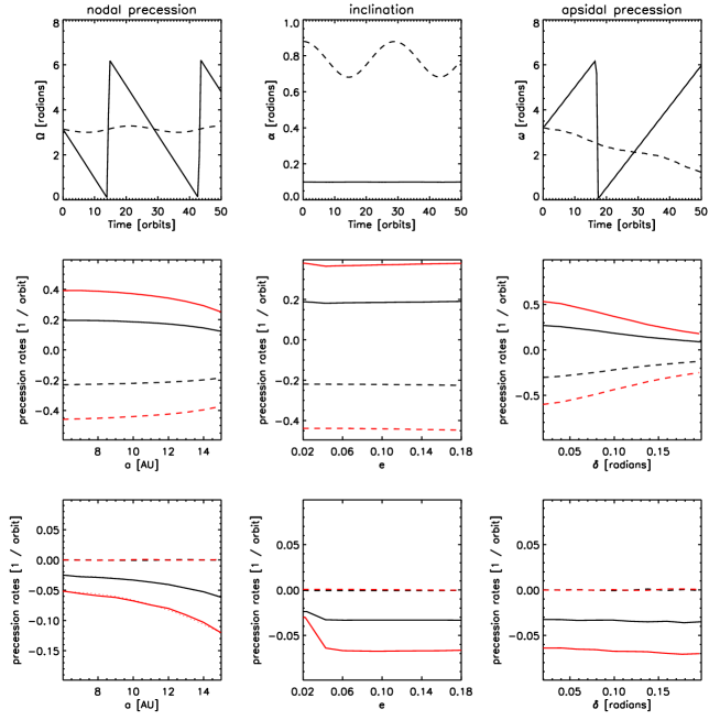
Figure 1: Upper panels: nodal (panel 1) and apsidal precession (panel 3) angles as well as inclination angles (panel 2) of a test particle experiencing the gravitational field of a disc and central star only. The solid lines show the results when viewed in a frame in which the disc is assumed to be coplanar with the reference plane. The dashed lines show the same quantities for the same model, but where the disc is now treated as if it was inclined by $\gamma_{F}=0.78\;(45^{\circ})$ to the reference plane, as it will be when the binary companion is included. Middle panels: nodal (dashed lines) and apsidal (solid lines) precession rates when the disc is highly inclined as a function of semi-major axis $a_{i}$ (panel 4), eccentricity $e_{i}$ (panel 5) and relative inclination $\delta_{i}$ (panel 6) for a standard disc mass (black) and a disc with the double mass (red). Bottom panels: nodal (dashed) and apsidal (solid) precession rates caused by the highly inclined disc as a function of semi-major axis $a_{i}$ (panel 7), eccentricity $e_{i}$ (panel 8) and relative inclination $\delta_{i}$ (panel 9) for a standard disc mass (black) and a disc with double that mass (red). In panel 7 a polynomial fit to the apsidal precession rates is shown (dotted lines).

If the inclination of the disc with respect to the binary plane becomes larger than the relative inclination of the particles ($\alpha_{d}\geq\delta_{i}$), however, the nodal and apsidal precession rates will be different.

In order to understand the effect of the gravity of a disc that is highly inclined with respect to our reference plane, we transform the planetesimal position and velocity vectors via the transformation given by Eq. (14), using a representative inclination of the disc of $\alpha_{d}=\gamma_{F}=0.78\;(45^{\circ})>\delta_{i}=0.1\;(5.7^{\circ})$ and assume that the disc is non-precessing with $\Omega_{d}=\Omega_{F}t=0$ (inclusion of a small precession frequency $\Omega_{F}\neq 0$ does not change the result.) The outcome of this transformation is shown by the dashed line in Fig.1 (panels 1-3) for the same reference particle as described earlier. We observe that the nodal precession $\Omega_{i}$ angle (panel 1) and inclination angle $\alpha_{i}$ (panel 2) are oscillating around a fixed value. This can be understood as follows. The angular momentum vector of the particle still precesses around the angular momentum vector of the disc as before. Unlike before, however, the disc has an inclination with respect to the reference plane of $\alpha_{d}=0.78\;(45^{\circ})>\delta_{i}$. Hence the precession of the particle angular momentum vector causes the measured inclination and nodal precession angles to oscillate around those of the disc, with an amplitude given by the particle’s relative inclination $\delta_{i}$. We verify that for the reference particle the nodal precession rate measured with respect to the disc midplane is $\dot{\Omega}\sim-0.23\;(-13.2^{\circ})$ per orbit, as seen from panel 4 (black dashed line). This corresponds to a precession period of 27 orbits, coinciding with the observed period of oscillation of the inclination and nodal precession angles measured with respect to the reference plane (panels 1 and 2, dashed line). Additionally, the particle appears to precess apsidally in a retrograde sense (panel 3, dashed line).

The precession rates (nodal and apsidal) are displayed as functions of semi-major axis, eccentricity and relative inclination in panels 7-9, respectively, for the highly inclined disc case, with the same line style and colour convention as used before. As can be seen from these panels, the net nodal precession rate is zero, since the disc causes oscillation but no net change of the nodal precession angle.

From panels 8-9 we observe that the apsidal precession rate is roughly independent of eccentricity $e_{i}$ and relative inclination $\delta_{i}$. However it depends on the semi-major axis, $a_{i}$, and also scales roughly with the disc mass, as shown in panel 7. For future purposes we fit this apsidal frequency by a second order polynomial:

$$\dot{\omega}=\frac{M_{d}}{\hat{M}}\left[C_{0}+C_{1}\left(\frac{a}{\rm AU}\right)+C_{2}\left(\frac{a}{\rm AU}\right)^{2}\right]\frac{1}{P_{d}}$$ (46)

with $C_{0}=-4.187\cdot 10^{-2}$, $C_{1}=5.118\cdot 10^{-3}$ and $C_{2}=-4.242\cdot 10^{-4}$. $P_{d}$ is the orbital period at the disc outer edge (which is nominally located at $r=10\equiv 20$ AU), $M_{d}$ is the disc mass and $\hat{M}$ is the nominal disc mass for the reference model introduced in Sect. 3.3. The fit is displayed in panel 7 (dotted lines) and matches the numerical data (solid line) well.

To summarise, the measured effect of the gravity of an inclined disc on the planetesimal orbit depends on the ratio of the inclination of the disc with respect to the binary plane, $\alpha_{d}$, and the inclination of the particle with respect to the disc, $\delta_{i}$. If $\delta_{i}\geq\alpha_{d}$ the resulting nodal and apsidal precession rates caused by the disc are displayed in Fig.1 (panels 4-6). If $\delta_{i}\leq\alpha_{d}$ the precession around the disc angular momentum vector causes oscillations in the nodal precession and inclination angles with an amplitude that is given by $\delta_{i}$. The apsidal precession in this case is displayed in Fig.1 (panels 7-9) and can be approximated by Eq. (46).

5 Planetesimal dynamics in inclined binary systems

Model	$\gamma_{F}$	$M_{d}$	$D$	$s_{i}$
label	[degrees]	[$\hat{M}$]	[AU]	[m]
1	0	1	60	10000
2	25	1	60	10000
3	45	1	60	10000
	45	1	60	1000
	45	1	60	100
4	45	3	60	10000
5	45	6	60	10000
6	45	1	90	10000
7	45	1	120	10000
8	25	1	60	100
	25	1	60	1000
	25	1	60	10000
9	45	1	60	100
	45	1	60	1000
	45	1	60	10000

Table 2: Table of runs: the first column gives the run label; the second column gives the inclination of the binary companion to the gas-plus-planetesimal disc, $\gamma_{F}$; the third column gives the disc mass in units of the reference mass; the fourth column gives the binary separation, $D$; the fifth column lists the planetesimal radii, $s_{i}$, included in the models.

We will now describe the dynamics of planetesimals that are orbiting in the full binary plus disc system. The model parameters are summarised in table 2. The planetesimals are initially set-up on circular, keplerian orbits that are coplanar with respect to the disc midplane (i.e. $\delta_{i}=0$). They are distributed radially in the interval $a_{i}\in[6,16]$ AU for models 1-7 (where the disc truncation radius is $\simeq 20$ AU). In an additional series of runs we confine the planetesimals to a narrow annulus with $\Delta a=10^{-3}$ AU centred around $a=10$ AU (models 8 and 9) to maximize the number of collisions and study collisional velocities in more detail.

We treat model 3 as our reference case. The inclination of the binary companion to the disc is initially set to $\gamma_{F}=0.78$ ($45^{\circ}$) and its separation from the central object is set to $D=60$ AU. The disc mass used in the reference model is $M_{d}=1\hat{M}$ and corresponds to a scaled minimum mass solar nebula as explained in Sect. 3.3. In the other models we varied the initial inclination $\gamma_{F}$ of the binary companion to the gas-planetesimal disc (models 1-3), the disc mass $M_{d}$ (models 4 and 5) and the binary separation $D$ (models 6 and 7).

5.1 Zero inclination case (model 1)

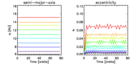
Figure 2: Orbital elements for the coplanar case. Panel 1 shows the semi-major axes of different planetesimals, where the colour convention introduced here is used in future plots. The eccentricity of the various planetesimals is shown in panel 2. The binary separaion $D=60$ AU.

In this model the binary orbital plane is coplanar with the planetesimal-plus-disc midplane. From time $t=0$ the planetesimals experience the gravity of the disc and gas drag forces (the planetesimals have size $s_{i}=10$ km), and the mass of the binary companion is increased to its final value over a time of four orbits. The evolution of the semi-major axes, $a_{i}$, and eccentricities, $e_{i}$, are shown in Fig.2. The colours correspond to different initial semi-major axes, with darker blue colours representing the inner planetesimals and the green-red colours representing planetesimals further out in the disc. We will also adopt this colour convention when discussing simulation results later in the paper. As can be seen from Fig.2 (panel 1), the binary companion does not change the semi-major axes of the bodies, as expected from secular theory. Eccentricities are generated, however, that are of the order of ($e_{i}\sim 10^{-2}$), as can be seen from Fig.2 (panel 2). Very modest eccentricities are generated because the planetesimals are orbiting in a slightly non-keplerian potential due to the disc gravity. But we also see that the eccentricities grow on a time scale of $\sim 5$ orbits due interaction with the binary whose mass grows over this time. The values of eccentricity obtained are consistent with those presented by Ciecieläg et al. (2007), who considered the evolution of planetesimals in a gas disc with a circular binary companion, but neglected the effects of disc gravity. Because of the closer proximity to the binary companion, the outer planetesimals are more strongly affected by these perturbations and their eccentricities are raised to larger values. Note that the data in this and the following figures has been smoothed over a temporal window of 1.8 orbits, but it is clear that after an initial rise, the eccentricities remain essentially constant for 80 orbits (7155 years).

Secular perturbations from an eccentric, coplanar binary companion lead to the generation of well-defined forced eccentricities, and can also lead to strong alignment of periastra for same-sized planetesimals in the presence of gas drag (Marzari & Scholl 2000; Thebault, Marzari & Scholl 2006). This causes a dramatic reduction in the impact velocities for these planetesimals. But this effect is absent for a circular companion as considered here, and eccentricities are largely generated by high frequency terms in the disturbing function. We find that the periastra are not well aligned near the beginning of the simulation, since a companion on a circular orbit cannot define a direction of preferred alignment (this effect may be seen in Fig. 7 later in the paper where we plot results for a simulation with a low inclination ($25^{\circ}$) binary companion). This basic point is in agreement with results presented by Ciecieläg et al. (2007), who also considered a circular binary. As such a binary companion on a circular orbit appears to be singular in its effect on the orbits of planetesimals embedded in a gas disc. This has potentially important consequences for the collisions between planetesimals reported later in this paper.

5.2 Low inclination case (model 2)

In this section we describe the simulation results for model 2, for which only planetesimals of size 10 km were considered and the binary inclination $\gamma_{F}=25^{\circ}$. Fig.3 shows the evolution of eccentricities $e_{i}$ (panel 1), nodal precession angles $\Omega_{i}$ (panel 2), inclinations $\alpha_{i}$ (panel 3) and relative inclinations $\delta_{i}$ (panel 4) for the different planetesimals using the same convention of colours as described in Sect. 5.1. As in the coplanar case, eccentricities are raised by interactions with the binary companion, but because the binary orbit is circular the forced eccentricity predicted by secular theory is negligible, and the eccentricities are generated by high frequency perturbations. We can observe that these are somewhat lower than in the coplanar case due to a reduced coplanar component of the companion’s gravity.

In panel 2 of Fig.3 we see that most of the planetesimals precess nodally at a joint rate with the disc, except for the outermost particle (red line), which will be discussed later in this section. This joint precession can be explained by the presence of the disc, with its gravitational field playing the major role. To illustrate this we also performed simulations of planetesimals that interact with the binary system only. The corresponding nodal precession and inclination angles of the planetesimals for such a simulation are shown in Fig.4.

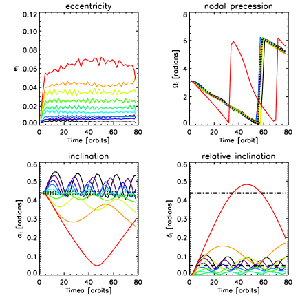
Figure 3: Orbital elements for the low inclination case $\gamma_{F}=25^{\circ}$. The colours represent planetesimals at different semi-major axes with the convention adopted from Fig.2. The eccentricity is depicted in panel 1. In panels 2 and 3 the nodal precession and inclination angles are shown, where the short dashed line represents the inner and outer edge of the disc. In panel 4 the relative inclination with respect to the disc is shown, where the short dashed line represents one pressure scale height and the dashed-dotted line indicates where $\delta_{i}=\alpha_{d}$. The binary separation $D=60$ AU.

Due to the secular perturbation of the secondary star alone, the inclinations are expected to stay constant while the orbital planes of the planetesimals precess at their free particle rate (Papaloizou & Terquem 1995):

$${\dot{\Omega}}_{i}^{free}=-\frac{3}{8\Omega_{K}}\frac{GM_{B}}{D^{3}}(3\cos^{2}{\alpha_{i}}-1).$$ (47)

which is a strong function of semi-major axis, as $\Omega_{K}\sim r^{-\frac{3}{2}}$ is the keplerian angular velocity. The left panel of Fig.4 shows that the nodal lines of the planetesimals become progressively randomised, leading to the dispersion of the planetesimal disk into a cloud of bodies surrounding the star, as found by Marzari, Thebault & Scholl (2009).

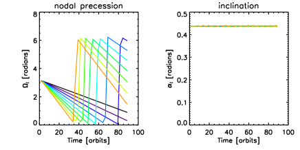
Figure 4: Simulation results of planetesimals interacting with the binary system only (no gas disc). The left panel shows the nodal precession, and the right panel shows the inclination.

Comparing this behaviour with the results displayed in Fig.3 (panels 2 and 3) we can see that the presence of the disc and its gravitational field causes fundamentally different behaviour of the planetesimals. The planetesimals remain coupled to the disc, as their nodal precession angles stay close to the disc precession angle (dashed line in panel 2 of Fig. 3). The role of gas drag in determining the relative inclination between the disc midplane and the planetesimals is negligible for this run for which the planetesimal size is 10 km. But for smaller planetesimals gas drag does play a role, as we will describe later in the paper.

In Fig.5 we show the time evolution of the nodal precession rates for the particle at $r=13.3$ AU (panel 1) and $r=6.2$ AU (panel 2). The various curves represent contributions due to gas drag (blue line), disc gravity (red line), binary companion (green line) and the total rate (black line) as calculated in Sect. 3.4. Because of its different radial location, the outer particle orbit precesses faster in the retrograde sense than the inner particle if the disc is absent. Confirming this we can observe in Fig.5 (panels 1 and 2) that $\dot{\Omega}_{i}$ due to the companion (green line) is about $\dot{\Omega}_{i}=-0.09\;(-5.15^{\circ})$ per orbit for the outer body, and $\dot{\Omega}_{i}=-0.03\;(-1.7^{\circ})$ per orbit for the inner body. It is the disc gravity, however, that compensates for this effect and causes the planetesimals to precess at a common net rate. Since the disc precesses rigidly at a rate $\dot{\Omega}_{D}\simeq\Omega_{F}=-0.06\;(-3.4^{\circ})$ per orbit, which corresponds to the free particle rate at about $a_{i}=11.5$ AU, disc gravity (red line) gives a positive contribution to the precession rate for the outer particle ($\dot{\Omega}_{i}>0$) and a net negative contribution for the inner particle ($\dot{\Omega}_{i}<0$). Since the particle-plus-disc system precesses in the retrograde sense the outer particle precession is slowed down, while the inner particle precession is speeded up by the disc, such that both bodies precess together with the disc on average at the rate $\Omega_{F}$. This result illustrates the fundamental importance of including the effects of disc gravity when calculating the dynamics of planetsimals in misaligned binary systems.

The nodal precession and inclination angles of the planetesimals show oscillations, as seen in Fig.3 (panels 2 and 3). These are caused by the disc gravity, as explained in Sect. 4 and illustrated by the red line in panel 5 of Fig. 5. The planetesimals effectively precess around the disc angular momentum vector at the same time as the disc-plus-planetesimal system precesses around the binary angular momentum vector. Initially the planetesimals are coplanar with the disc midplane ($\delta_{i}=0$), but as the system evolves during early times, differential nodal precession between particle $i$ and the disc occurs, leading to a build up of relative inclination $\delta_{i}$, since $\delta_{i}^{2}\propto(\Omega_{i}-\Omega_{d})^{2}$ as shown by Eq. (16). The differential precession is greatest for planetesimals whose semi-major axes deviate most from $a=11.5$ AU (the radius at which planetesimals naturally want to precess at the same rate as the disc), so the relative inclination is largest for particles that are furthest inside (black line) or outside (yellow line) this value, as demonstrated in panel 4 of Fig. 3.

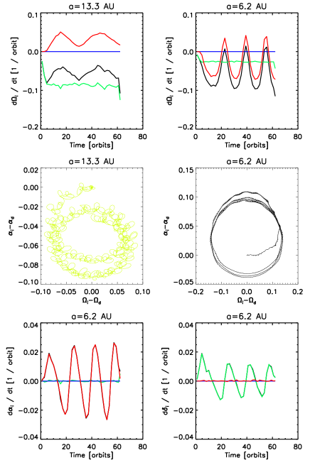
Figure 5: Panels 1 and 2 show the nodal precession rates of a planetesimal with semi-major axis at $a_{i}=13.3$ AU (panel 1) and $a_{i}=6.2$ AU (panel 2). Shown are the contributions of the disc gravity (red line), binary companion (green line), gas drag (blue line) and total rate (black line). In panels 5 and 6 we also show the rates of inclination change with respect to the binary and disc midplane respectively for the inner particle. In panels 3 and 4 the trajectory of the tip of the particle’s angular momentum vector is shown projected onto the ($\Omega_{i}-\Omega_{d}$, $\alpha_{i}-\alpha_{d}$) plane for the outer (panel 3) and inner particle (panel 4).

The disc model has an aspect rato $H/R=0.05$, so that planetsimals which develop relative inclinations $\delta_{i}>0.05$ will spend large fractions of their orbits away from the disc midplane. Planetesimals interior to $8$ AU and exterior to $13$ AU have relative inclinations $\delta_{i}\simeq 0.1$, and so spend large fractions of their orbits essentially outside of the disc. We also observe that the oscillation periods of the inclination, $\alpha_{i}$, and nodal precession angles, $\Omega_{i}$, varies among the planetesimals. This is expected due to their different semi-major axes and relative inclinations, and the observed periods are all consistent with Fig.1 (dashed lines in panels 4-6), which we recall shows how the disc alone acts on the planetesimals.

We note that the inclination oscillations, seen in Fig.3 (panel 3), begin in opposite senses for planetesimals whose semi-major axes are above or below $a=11.5$ AU (i.e. planetesimals below $a=11.5$ AU are perturbed onto higher inclination orbits, while planetesimals exterior to $a=11.5$ AU are perturbed onto lower inclination orbits). Panel 3 of Fig.5 plots the inclination angle difference $\alpha_{i}-\alpha_{d}$ versus the precession angle difference $\Omega_{i}-\Omega_{d}$ for a planetesimal located at 13.3 AU. A similar plot for a planetesimal at 6.2 AU is shown in panel 4. Each plot shows the trajectory of the tip of the planetesimal angular momentum vector relative to the disc angular momentum vector (which is located at the origin). For the inner particle the companion induces a differential precession $\Omega_{i}-\Omega_{d}>0$ and the anti-clockwise precession around the disc angular momentum vector causes the planetesimal to approach a higher inclination orbit $\alpha_{i}-\alpha_{d}>0$ during the first half of this precession cycle. For the outer planetesimal the induced differential precession is $\Omega_{i}-\Omega_{d}<0$, and the anti-clockwise precession causes perturbation onto a lower inclination orbit $\alpha_{i}-\alpha_{d}<0$.

We now return to the planetesimal that is orbiting at $a=15$ AU. This body shows quite distinct behaviour from all the other bodies, as shown in Fig.3 (red lines). This particle is dominated by the gravity of the companion, and it nodally precesses fast enough to decouple from the disc. As it precesses away from the disc, the relative inclination $\delta_{i}$ grows (panel 4 of Fig.3). The precession rate around the disc angular momentum vector is a decreasing function of relative inclination, so the precession period becomes long for this particle. Because $\Omega_{i}-\Omega_{d}<0$, we observe the quasi-monotonic decrease of inclination in panel 3 of Fig.3 until the reversal point at $t=47$ orbits, when the differential nodal precession is $\Omega_{i}-\Omega_{d}=\pi$. The planetesimal orbital plane then approaches the disc midplane from the other side ($\Omega_{i}-\Omega_{d}>0$), and we observe the quasi-monotonic increase of inclination after $t=47$ orbits.

Over longer time scales than we have been able to consider because of the computational expense of running the simulations, we expect the outermost planetesimals which decouple from the disc to show continued oscillations in their inclinations, with an oscillation period equal to the synodic precession period. Ignoring the possible growth of planetesimals into planets, or their collisional destruction, those bodies which remain almost coplanar with the disc should continue to do so over long time scales until the disc mass decreases due to viscous evolution and/or photoevaporation. Significant reduction of the disc mass would eventually allow the planetesimal dynamics to become dominated by the companion star, and they would decouple from the disc. But, we also note that that the disc and binary orbit plane will evolve toward alignment on the viscous evolution time at the outer edge of the of the disc (Terquem et al. 1999; Larwood et al. 1996; Fragner & Nelson 2010). So it is possible that an initially misaligned protoplanetary disc may align significantly over its lifetime, bringing with it any planetary system which has formed within it. The final degree of misalignment for a planetary system formed in an inclined protoplanetary disc may therefore be substantially less than the initial misalignment of the protostellar disc.

5.2.1 Collisional velocities in low inclination case (model 7)

In this section we present the results of a simulation which examines collisions between planetesimals in a system where the binary companion has an inclination of $\gamma_{F}=25^{\circ}$ relative to the disc midplane. To increase the collision rate to statistically meaningful values which can be measured in a simulation, we initialise the planetesimals with a narrow range of semi-major axes ($\Delta a=10^{-3}$ AU) centred around $a=10$ AU. We consider three different planetesimal sizes (100m, 1km and 10km), and for each size we include 50 particles. We check the condition for orbital crossing given by Eq. (28) every 100 time steps for each of the 11175 particles pairs (100 time steps corresponds to 0.011 orbital periods at 10 AU, the orbital radius of the planetesimals). If the orbit crossing condition is satisfied, then we calculate the velocity at the crossing point for both planetesimal orbits according to Eq. (LABEL:velocity).

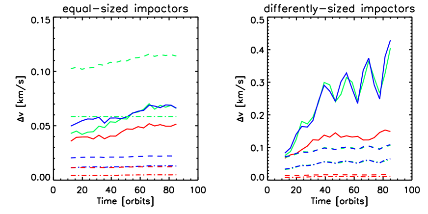
Figure 6: Average collisional velocities in the low inclination $\gamma_{F}=25^{\circ}$ case between equally sized (left panel) and differently sized planetesimals (right panel) for planetesimals centred around 10 AU from the central star. Left panel: collisions between 10km-10km bodies (green-solid); 1km-1km (blue-solid); 100m-100m (red-solid). Right panel: collisions between 10km-1km bodies (green-solid); 10km-100m (blue-solid); 1km-100m (red-solid). Threshold velocities for catastrophic disruption corresponding to the different size-combinations for the weak (dash-dotted line) and strong aggregates (dashed line) are also shown.

Before discussing the results of model 7, it is worth recapping what we might expect based on previous work in which the gravity of the disc was neglected. Same-sized planetesimals being perturbed by an eccentric, coplanar binary companion will experience a growth in their forced eccentricity, but gas drag damping will cause strong orbital phasing dramatically reducing collisional velocities (Marzari & Scholl 2000; Thebault, Marzari & Scholl 2006). The different phasing of pericentres for planetesimals of different size, however, leads to large collision velocities which are likely to be disruptive. The inclusion of a small inclination ($\alpha_{i}\leq 5^{\circ}$) causes different sized planetesimals to orbit in different planes, such that collisions between similar sized bodies are more frequent than between different sizes. The fact that the pericentre phasing is maintained in this scenario means that planetesimal growth may be more likely to occur in inclined systems (Xie & Zhou 2009).

The collision velocities we obtain are shown in Fig.6 (solid lines) for collisions between equally sized (panel 1) and differently sized planetesimals (panel 2). As mentioned in Sect. 5.1, an important difference between our set-up and previous work is that we consider a circular, inclined binary companion, resulting in a broad distribution of planetesimal longitudes of pericentre, $\omega_{i}$, even for planetesimals of the same size. Consequently, we see that the collision velocities for equal sized bodies in panel 1 are quite large, being between 50 - 70 ms^-1 at the end of the simulation. Although it appears that the circular binary is largely responsible for the growth of eccentricity and the misaligned periastra of orbits for same sized planetesimals, it is possible that gravitational perturbations associated with spiral waves in the disc also contribute. The collision velocities for differently sized bodies, however, are even larger than for same-sized bodies, and exceed 400 ms^-1 after 80 orbits (see panel 2).

Fig.7 shows averages of all the quantities that determine the relative velocities according to the analytical estimate given by Eq. (44), and we can use this data to determine the main contributors to the collision velocities shown in Fig.6. Panel 1 shows the difference of longitude of pericentre $\Delta\omega_{i}$, panel 2 shows the average eccentricity $e$, panel 3 shows the difference in eccentricity $\Delta e_{i}$, panel 4 shows the difference in inclination $\Delta\alpha_{i}$, panel 5 shows the angle between the nodal lines $\Delta\Omega_{i}$ and panel 6 shows the average inclination $\alpha_{i}$. Note that these averages were obtained only for orbits which mutually cross, and do not represent the distributions for the whole ensemble of particles. Using the numbers extracted from these figures in Eq. (44) we can reproduce the relative velocities shown Fig.6 with good accuracy, indicating that Eq. (44) is a valid approximation and that our collision detection technique is generating collision velocities which are consistent with expectations.

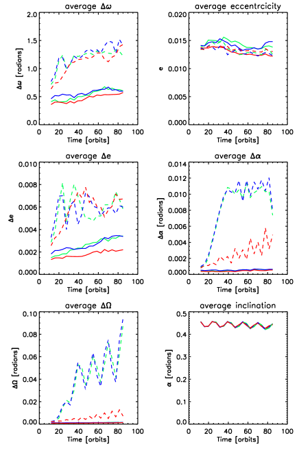
Figure 7: Average orbital parameters of the colliding planetesimal pairs in the low inclination $\gamma_{F}=25^{\circ}$ case. The line colours and styles are as follows: green-solid (10km-10km); blue-solid (1km-1km); red-solid (100m-100m); green-dashed (10km-1km); blue-dashed (10km-100m); red-dashed (1km-100m).

For collisions between planetesimals of the same size the dominating contribution to the square of the relative velocity comes from the term which is proportional to $e_{i}^{2}\Delta\omega_{i}^{2}$, while all other terms are at least an order of magnitude smaller. This implies that planetesimals with the same size all orbit more or less in the same plane (as shown by panels 4 and 6), and relative velocities are generated due to misalignment of their orbit pericentres, $\Delta\omega_{i}$, a result which is broadly consistent with those obtained by Xie & Zhou (2009). We note that our collision detection method is not strictly valid in this regime, because it predicts the locations of the orbit crossing points incorrectly for coplanar orbits. But, because the average pericentre misalignment is on the order of unity (measured in radians), the average collision velocities reported by the algorithm are consistent with the analytical prediction $v_{coll}\simeq e\,\Delta\omega$ to within a factor of order unity. Under these conditions, incorrect detection of the orbit crossing locations still leads to estimates of the average collision velocities being approximately correct.

Although panel 1 of Fig.7 shows that the misalignment of pericentres increases slightly over time when considering only those particles whose orbits intersect, we find that the average pericentre misalignment calculated over all same-sized particle pairs actually decreases during the simulation. The reason for this is not clear, but it is interesting to note that even when the binary orbit is circular, the long term evolution appears to be toward one where the pericentres tend toward alignment, and this effect is most marked for the smallest planetesimals suggesting that it is an effect due to gas drag.

As seen in panel 2 of Fig.6, planetesimals of different sizes tend to have much larger collisional velocities. One reason is the increased misalignment of pericentres, as can be observed in Fig.7 (panel 1, dashed lines). This may be a direct consequence of gas drag, as discussed in previous work (Marzari & Scholl 2000; Thebault, Marzari & Scholl 2006), but it may also be due to the fact that particles which experience stronger gas drag orbit closer to the disc midplane than larger planetesimals do. This then affects the gravitational perturbations experienced by the particles as they travel through the disc, which may increase the pericentre misalignment. But a more important contribution to the square of the relative velocities comes from the term $\propto\sin^{2}{(\alpha_{i})}\Delta\Omega_{i}^{2}$. We find that due to the different gas drag strengths, planetesimals of different sizes tend to precess nodally at different rates for some initial time until disc gravity causes them to precess together with the disc. While smaller planetesimals tend to precess together with the disc immediately and consequently their relative inclinations stay low, larger planetesimals tend to precess at their own free particle rates for a longer time, causing a larger build up of relative inclination. In other words, although the planetesimal swarm as a whole is forced on average to precess with the disc by the disc gravity, smaller planetesimals oscillate about the midplane of the disc with a smaller amplitude than larger planetesimals. This induces a large misalignment of their orbital planes $\Delta\Omega_{i}$ as seen in panel 5 of Fig.7 (dashed lines) in addition to the misalignment of their pericentres.

The frequency of collision between bodies is an important factor during the growth of planetesimals, and Xie & Zhou (2009) have suggested that the differential phasing of nodal lines for planetesimals of different sizes may increase the relative importance of collisions between similar sized objects rather than different sized bodies. We have examined the collision frequency reported by our collision detection technique by simply counting the number of orbit crossing events reported during the simulation. In basic qualitative agreement with Xie & Zhou (2009), we find that the collision frequency during the simulation between same-sized objects is a factor of 3 - 6 times larger than between different sized objects. Our results thus support the idea that planetesimal growth in inclined binaries is likely to proceed via accretion of similar sized bodies.

We conclude that relative velocities between differently sized planetesimals tends to be large in binary systems whose orbital plane is misaligned with the planetesimal-plus-disc plane, while relative velocities between same sized planetesimals are largely unaffected by this non-coplanarity. But the circular orbit of the binary companion prevents strong pericentre alignment for similar sized bodies, leading to significant collisional velocities in this case too, in contrast to the situation observed when the companion is on a coplanar eccentric orbit. The question of what happens in the case of an eccentric, inclined companion unfortunately goes beyond the scope of this paper but should obviously be the focus of future work.

We now want to determine whether the collisional velocities seen in Fig.6 will lead to growth or erosion of the planetesimals. In principle there are three possible outcomes: accretion, in which the largest body involved in the collision contains more mass after the collision; catastrophic disruption, in which more than half of the total mass of the system is dispersed after the collision; erosion (or cratering), where the largest body loses a small amount of mass during the collision. Only accretion leads to the growth of a planetesimal.

For simplicity in interpreting our results, we adopt the universal law for the largest remnant mass from Stewart & Leinhardt (2009):

$$\frac{M_{lr}}{M_{tot}}=1-\frac{1}{2}\frac{Q_{R}}{Q_{D}},$$ (48)

where $M_{lr}$ is the mass of the largest post-collision remnant, and $M_{tot}=M_{1}+M_{2}$ is the total mass of the two colliding bodies $M_{1}$ and $M_{2}$. The quantity $Q_{R}=0.5\frac{M_{1}M_{2}}{M_{tot}^{2}}\Delta v^{2}$ is the reduced mass kinetic energy scaled by the total mass of the colliding system. For equally sized bodies accretional collisions require $\frac{M_{lr}}{M_{tot}}>\frac{1}{2}$, from which it follows that $Q_{R}<Q_{D}$. Hence $Q_{D}$ is called the catastrophic disruption limit of the collisions (the energy required to disperse half the total mass). If $Q_{R}>Q_{D}$ collisions between equally sized bodies lead to catastrophic disruption. When considering collisions between differently sized bodies the condition has to be modified. Let $M_{1}\gg M_{2}$ such that $M_{2}=\mu M_{1}$ with $\mu\ll 1$. The condition for accretion is now $M_{lr}>M_{1}$, from which it follows that $Q_{R}<\left(\frac{2\mu}{1+\mu}\right)Q_{D}$, which implies for the relative velocity threshold:

$$\delta v_{D}=2\sqrt{1+\mu}\sqrt{Q_{D}}$$ (49)

The disruption limit $Q_{D}$ is sensitive to factors that influence the energy and momentum coupling between the colliding bodies (i.e. impact velocity, mass ratio and material properties such as strength and porosity). Stewart & Leinhardt (2009) show that the catastrophic disruption curve $Q_{D}$ can be fit to an analytical formula (Houssen & Holsapple 1990,1999):

$$Q_{D}=\left[q_{S}R_{12}^{9\mu_{M}/(3-2\phi_{M})}+q_{G}R_{12}^{3\mu_{M}}\right]V_{I}^{(2-3\mu_{M})}$$ (50)

where $\mu_{M}$ and $\phi_{M}$ are material properties. In this expression $R_{12}$ is the spherical radius of the combined mass $M_{tot}$ assuming a density of $\rho_{s}=1$ g cm^-3. Since we use a density of $\rho_{s}=2$ g cm^-3 this radius is given by $R_{12}=2^{\frac{1}{3}}(1+\mu)^{\frac{1}{3}}R_{1}$, where $R_{1}$ is the spherical radius of the larger mass $M_{1}$ involved in the collision. The first term on the right hand side of Eq. (50) represents the strength regime, while the second term represents the gravity regime. Very small bodies are supported by material strength (first term), which decreases as the planetesimal size increases. As gravity becomes more important for larger bodies the second term becomes dominant and increases the disruption limit again.

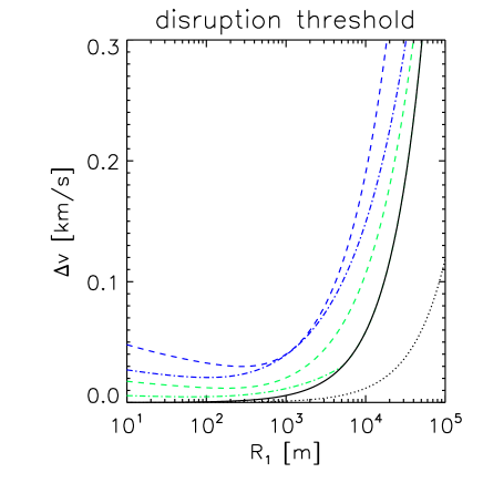
Figure 8: Threshold velocities for collisions between equally sized planetesimals as a function of their spherical radius $R_{1}$. The disruption curves for the weak (dashed-dotted line) and strong rock (dashed line) are shown for two different impact velocities $V_{I}=50$m/s (green) and $V_{I}=2$km/s (blue) along with the solution for rubble piles (black-solid line). The bodies escape velocity (black-dotted line) is also shown.

Stewart & Leinhardt (2009) derive the constants $q_{S}$, $q_{G}$, $\mu_{M}$ and $\phi_{M}$ for weak aggregates, such as weak rock and porous glass, by fitting the disruption curve to their numerical results. For weak aggregates they find (in cgs units) $q_{S}=500$, $q_{G}=10^{-4}$, $\mu_{M}=0.4$ and $\phi_{M}=7$. For strong rocks they use the basalt laboratory data and modelling results from Benz & Asphaug (1999), and find $q_{S}=7\cdot 10^{4}$, $q_{G}=10^{-4}$, $\mu_{M}=0.5$ and $\phi_{M}=8$. In the limit of very large bodies the disruption curve can be best fitted by their results of colliding rubble piles. In this regime Stewart & Leinhardt (2009) find

$$Q_{RP}=1.7\cdot 10^{-6}R_{12}^{2}$$ (51)

for equal mass bodies and a factor of about three larger than this if the impactor size is much smaller than the target size. For illustrative purposes we present the relative velocity threshold $\delta v_{D}$ obtained by combining Eq. (49) and Eq. (50) in the case of identical colliding bodies ($\mu=1$) in Fig.8. Note that in the limit of large bodies at low impact velocities, we set $Q_{D}=Q_{RP}$, because the rubble-pile solution for equal mass bodies defines a lower limit for disruption in this regime. The figure shows the limiting velocity below which collisions will lead to net accretion as a function of the planetesimal radius $R_{1}$ for the weak (dashed-dotted line) and strong aggregates (dashed line) at two different impact velocities $V_{I}=2$km/s (blue line) and $V_{I}=50$m/s (green line). It is apparent that the threshold velocity is increased for larger impact velocities as more energy is partitioned into shock deformation. In contrast, at low impact velocities the momentum coupling between the colliding bodies is more efficient and less energy is needed to cause erosion of planetesimals. As gravity becomes more important than strength for very large bodies the curves join onto the disruption curve for colliding rubble piles (black solid line). In this regime the threshold velocity is about a factor of 3-5 larger than the escape velocity from the bodies surface (dotted line).
To compare the relative velocities obtained from our numerical simulations with the disruption threshold velocity, we evaluate Eq. (49) for equally ($\mu=1$) and differently sized $\mu=10^{-3}$ planetesimals using $V_{I}=\Delta v$ in Eq. (50) and choosing $R_{1}$ as the bigger of the two planetesimals involved in the collision. If the rubble-pile disruption limit gives a higher estimate for a given size combination we use this limit instead.

We note that Stewart & Leinhardt (2009) considered target-projectile mass ratios only down to 0.03, instead of the values $10^{3}$ and $10^{6}$ that apply to collisions of 1km or 100m sized bodies with a 10km sized target. As such we are applying the Stewart & Leinhardt (2009) results in a regime where catastrophic disruption is unlikely to occur, and therefore outside of the regime of validity of their study, strictly speaking. Nonetheless, it reasonable to assume that even if catastrophic disruption does not occur during high velocity impacts, accretional growth is also unlikely due to erosion.

The results are plotted in Fig.6 for the strong (dashed line) and weak aggregates (dashed-dotted line). Except for collisions between equally sized $10$km bodies (green), the collisional velocities are always substantially larger than the erosion/disruption threshold. Hence we conclude that growth of planetesimals probably can not occur for planetesimal sizes $<10$km. For the equally ($10$km) sized bodies on the other hand the situation is not as clear. Although the collisional velocities lie below the strong aggregate threshold (green dashed line) they are also slightly above the weak aggregate threshold (dashed-dotted line). This suggests that collisions might also lead to erosion in this size regime. But it should be noted that we have not included a realistic planetesimal size distribution in these simulations, and it is possible that collisions between planetesimals clustered in size around 10km, whose orbit planes are very modestly inclined with respect to one another, may allow accretion to occur for strong aggregates. Examination of this possibility will require future simulations that adopt a more realistic and continuous size distribution.

If collisions between $10$km sized planetesimals do lead to growth then this will most definitely not occur in the standard runaway regime, because the escape velocity is $\sim 10$m/s. It is possible, however, that type II runaway growth may occur (Kortenkamp et al. 2001) in which the large velocity dispersion causes growth to be orderly while the bodies remain small, but enters a runaway phase when large bodies form whose escape velocities are larger that the velocity dispersion. We conclude that in an inclined binary system on a circular orbit, relative velocities are excited that will lead to erosion of planetesimals for sizes $\leq 10$km which we have considered here, and growth is uncertain for 10km sized bodies.

5.3 High inclination cases and the Kozai effect

For large inclinations between the binary and planetesimal orbital planes, it is possible that the Kozai effect will switch on, causing cyclic variations of planetesimal eccentricities and inclinations (Kozai 1962). In this section we describe this effect in more detail in order to simplify the understanding of results which are described later in this paper. The equations describing the secular evolution of the inclination $\alpha_{i}$, eccentricity, $e_{i}$, and longitude of pericentre, $\omega_{i}$, can be written as (Innanen et al. 1997):

$$\frac{\partial\alpha_{i}}{\partial\tau} = -\frac{15}{8}\frac{e_{i}^{2}\sin{(2\omega_{i})}\sin{(\alpha_{i}})\cos{(\alpha_{i})}}{\sqrt{1-e_{i}^{2}}}$$ (52)

$$\frac{\partial e_{i}}{\partial\tau} = \frac{15}{8}e_{i}\sqrt{1-e_{i}^{2}}\sin{(2\omega_{i})}\sin^{2}{(\alpha_{i})}$$ (53)

$$\frac{\partial\omega_{i}}{\partial\tau} = \frac{3}{4}\sqrt{1-e_{i}^{2}}\left\{2(1-e_{i}^{2})+5\sin^{2}{(\omega_{i})}\left[e_{i}^{2}-\sin^{2}{(\alpha_{i})}\right]\right\}$$ (54)

where for simplicity of notation we have introduced the time variable:

$$\tau=[D^{3}\Omega_{Ki}/GM_{B}]^{-1}t.$$ (55)

Hence the time scale on which any of the given quantities change is $\propto D^{3}$. It can be seen from Eq. (54) that there is a value of $\omega_{i}$ for which $\dot{\omega}_{i}=0$. To lowest order in $e_{i}$ this occurs when

$$\sin^{2}{(\omega_{i})}=\frac{2}{5\sin^{2}{(\alpha_{i0})}}$$ (56)

where $\alpha_{i0}$ is the initial inclination of planetesimal $i$. Having obtained this value, the apsidal precession is halted, as $\dot{\omega}_{i}=0$. This leads to the exponential growth of eccentricity. To illustrate this we can substitute Eq. (56) into Eq. (53) to find:

$$\frac{\partial e_{i}}{\partial\tau} = \frac{15}{4}\sin^{2}{(\alpha_{i0})}\sin{(\omega_{i})}\cos{(\omega_{i})}e_{i}$$ (57)

$$= \frac{15}{4}e_{i}\sqrt{\frac{2}{5}\left[\sin^{2}{(\alpha_{i0})}-\frac{2}{5}\right]}.$$

Hence the Kozai effect is only active for initial inclinations $\sin{(\alpha_{i0})}\geq\sqrt{\frac{2}{5}}$ or written differently $\alpha_{i0}\geq 0.68$ radians. The critical angle for which the Kozai effect switches on is thus $\alpha_{K}=39.2^{\circ}$. Additionally it can be shown that the Delaunay variable, $D_{i}$, (which is equivalent to the component of the planetesimal angular momentum which is parallel to the binary angular momentum vector) is a constant of the motion, where $D_{i}$ is defined by

$$D_{i}=\sqrt{a_{i}(1-e_{i}^{2})}\cos{(\alpha_{i})}.$$ (58)

As secular variations do not change the semi-major axes, this implies that an increase in eccentricity is coupled to a decrease in inclination, and vice versa.

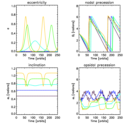
Figure 9: Orbital elements of planetesimals with different initial inclinations interacting with the binary system only. Panel 1 shows the eccentricity and panel 2 shows the nodal precession angle. The inclination with respect to the binary plane and the longitude of pericentre (apsidal precession) are depicted in panels 3 and 4, respectively.

To study the Kozai effect in the absence of the disc, we have performed N-body simulations of planetesimals interacting with the binary system only. The results are depicted in Fig.9 for planetesimals with various initial inclinations. It can be seen that the eccentricities and inclinations undergo cyclic variations for planetesimals whose initial inclination are $\alpha_{i}\geq\alpha_{K}$ (yellow, green and light blue lines in Fig.9). This can be explained as follows. As the eccentricity grows and the inclination decreases (panels 1 and 3), the latter eventually hits the Kozai threshold, $\alpha_{K}$, at which point there is no value for $\omega_{i}$ for which expression (56) holds. Consequently $\dot{\omega}_{i}\neq 0$ and $\omega_{i}$ evolves to values for which $\dot{e}_{i}\leq 0$ and $\dot{\alpha}_{i}\geq 0$. Hence, eventually $\dot{\omega}_{i}=0$ can be obtained again, but now for a value of $\omega_{i}$ which is causing the opposite evolution of eccentricities and inclinations until the original configuration is recovered and the Kozai-cycle is completed. We can clearly see in Fig.9 how the increase or decrease of eccentricities and inclinations is connected to the halting of apsidal precession during each half-cycle of the Kozai mechanism (panel 4). Additionally, we observe that the time scale on which the eccentricities and inclinations vary are increased as the initial inclination $\alpha_{i0}$ is decreased. Once the initial inclination is $\alpha_{i0}<\alpha_{K}$ (Fig.9, blue and black lines) the condition $\dot{\omega_{i}}=0$ can never be obtained. Consequently there are no net changes in eccentricities and inclinations and the Kozai effect is switched off.

5.4 High inclination case (model 3)

In model 3 we increased the inclination between the disc-planetesimal system and the binary plane to $\gamma_{F}=0.78$ ($45^{\circ}$). As described in the previous section, once the inclination exceeds a critical value $\alpha_{K}=0.68$ ($39.2^{\circ}$), the Kozai effect may lead to large eccentricity and inclination variations of the planetesimals, provided the disc mass is not too large (see later for a discussion about the conditions under which the Kozai effect operates).

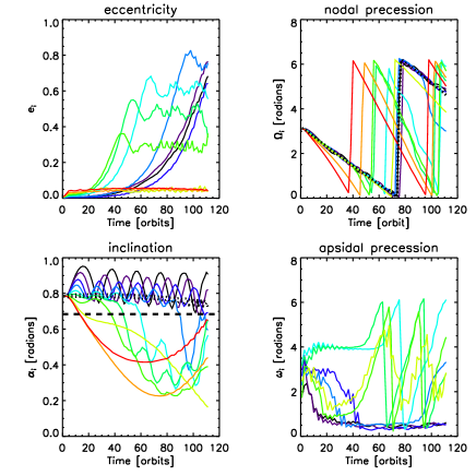
Figure 10: Orbital elements for the highly inclined case $\gamma_{F}=0.78\;(45^{\circ})$ (model 3). Panel 1 shows the eccentricity grows due to the Kozai effect for all but the outermost planetesimals . The nodal precession and inclination angles are depicted in panel 2 and 3, respectively, where the short dashed lines represent the inner and outer disc edge. The long dashed line in panel 3 represents the threshold inclination of $\alpha_{K}=39.2^{\circ}$ above which the Kozai mechanism is expected to operate. The apsidal precession angles are depicted in panel 4.

The presence of our scaled minimum mass solar nebula disc does not prevent the onset of the Kozai effect for planetesimals with semi-major axes $a<12$ AU, as seen from Fig.10 (panels 1 and 3), where we use the same colour convention for depicting the planetesimals as a function of initial semi-major axis as in models 1 and 2.

The eccentricity grows earliest for planetesimals with larger semi-major axes (panel 1, green lines). When the Kozai mechanism starts operating, the inclination starts to decrease. In the absence of the disc, this decrease would continue until the threshold of $\alpha_{K}=0.68\;(39.2^{\circ})$ is approached, after which the inclination would increase and the eccentricity would decrease again. In the presence of the disc, however, the situation is different. As the Kozai effect reduces the inclination, $\alpha_{i}$ the nodal precession induced by the binary accelerates according to Eq. (47). This causes the planetesimal orbits to become significantly inclined relative to the disc midplane (see panel 3 of Fig.10). Concurrent precession about the disc angular momentum vector due to the disc gravity causes a quasi-monotonic decrease of inclination relative to the binary. The planetesimals are thus perturbed by the disc onto orbits with inclination $\alpha_{i}<\alpha_{K}$, causing the Kozai effect to switch off. At this stage the planetesimal has only completed a portion of its Kozai cycle and is left with high eccentricity (panel 1) and a reduced inclination (panel 3), at least for the duration of the simulation. The apsidal precession angles are depicted in panel 4 of Fig.10. During the time when the Kozai effect is operating ($\alpha_{i}>\alpha_{K}$), the apsidal precession is halted such that $\dot{\omega}_{i}=0$. After the Kozai effect has switched off ($\alpha_{i}<\alpha_{K}$) we observe prograde apsidal precession ($\dot{\omega_{i}}>0$). Although this precession rate is dominated by the perturber the disc enhances the prograde precession rate, since $\delta_{i}>\alpha_{d}$ at this stage. The total rate is thus given by the sum of contributions by the binary companion and disc.

Planetesimals with semi-major axes $a_{i}>12$ AU decouple from the disc due to the differential precession induced by the binary companion. Consequently their inclinations get perturbed below $\alpha_{K}$ before the Kozai effect can start to operate, and their eccentricities stay low, at least for the duration of the simulations that we present here.

The simulation presented in Fig.10 was only run for 110 orbits measured at the disc outer edge ($\sim 10^{4}$ years). Those planetesimals which have experienced the Kozai effect have only undergone half a Kozai cycle, which stalls because the inclination falls below $\alpha_{K}$. But we see in panel 3 that the inclination relative to the binary is increasing toward $\alpha_{K}$ at the point when the simulation ends, because the planetesimals have precessed nodally by more than $180^{\circ}$ with respect to the disc. We would therefore expect that the Kozai effect will switch on again when $\alpha_{i}>\alpha_{K}$, allowing the previous Kozai cycle to complete. Similarly, we see that the inclinations of the planetesimals located beyond 12 AU are also increasing toward $\alpha_{K}$, such that the Kozai effect will switch on for them eventually. A long term effect of the disc thus appears to be to prolong the period associated with the Kozai cycles because of its effect on the planetesimal inclinations. An important consequence of this is that it increases the dephasing of the Kozai cycles at different locations in the disc, ensuring that over long times planetesimals with different semi-major axes are at very different phases of their Kozai cycles. There will therefore be very large variations in both eccentricity and inclination within the planetesimal swarm, leading to very large collisional velocities between planetesimals that are well separated in their semi-major axes.

5.4.1 Varying planetesimal sizes (model 3)

In the previous discussion we focused on planetesimals with size $s_{i}=10$km, for which the gas drag forces are very weak. As we decrease the size of the bodies in the system, the gas drag becomes more important since the stopping time is $\propto s_{i}$. Results for the 1km and 100m sized planetesimals are shown in the left and right panels of Fig.11 respectively.

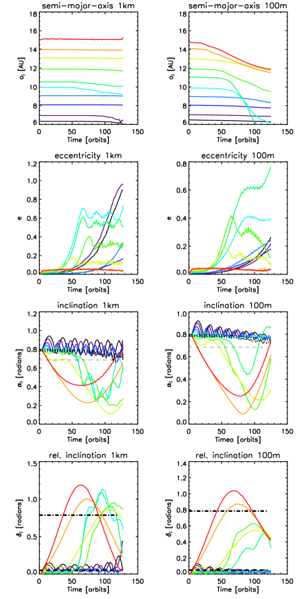
Figure 11: Orbital elements for the 1km (left panels) and 100m sized planetesimals (right panels). The semi-major axes are shown in panels 1 and 2. In panels 3 and 4 eccentricity growth due to the Kozai effect is still apparent for both planetesimal sizes. The inclination is shown in panels 5 and 6, where the short dashed lines represent the disc inner and outer edge, and the long dashed line marks the threshold inclination above which the Kozai effect operates. In panels 7 and 8 the relative inclination with respect to the disc is shown, where the short dashed line indicates the one pressure scale height limit for the gas disc. The dash-dotted line represents the inclination of the binary orbit plane relative to the disc midplane.

The Kozai effect leads to the growth of eccentricities (panels 3 and 4) and relative inclinations (panels 7 and 8) for both particle sizes shown. This is not surprising, since the time scale on which we expect substantial damping of eccentricity and inclination to occur is of the order of the gas drag stopping time. For our disc model this is given by:

$$\tau_{S}=0.81\left(\frac{s_{i}}{{\rm m}}\right)\left(\frac{a}{\rm AU}\right)^{2}\;P_{d},$$ (59)

where $s_{i}$ is expressed in metres. For the $100$m sized planetesimals at $a=6-15$ AU the stopping time is of the order of $10^{3}-10^{4}$ orbits, respectively, and is a factor of $10$ longer for the $1$km sized planetesimals. This is much longer than the time scale on which the Kozai effect operates ($\sim 10^{2}$ orbits), and hence we would not expect the gas drag to prevent growth of eccentricity and relative inclination in this size range. We comment here (without showing results), that we also found the Kozai effect to operate for $10$m sized bodies, for which the drag and Kozai time scales are similar.

The increased effect of gas drag causes the semi-major axes to decay (see panels 1 and 2 in Fig.11). As planetesimals experience the Kozai effect, and develop large eccentricities and relative inclinations, their relative velocities with respect to the gas disc becomes very large (since $|{\bf v}_{i}-{\bf v}|^{2}\simeq v_{K}^{2}\left(e_{i}^{2}+\delta_{i}^{2}\right)$ from expression [45]). As they travel through the disc they lose kinetic energy rapidly to the gas, and their semi-major axes decay. We note that those 100m sized bodies lying beyond 12 AU, which do not experience the Kozai effect during the simulation, also undergo rapid decay in their semi-major axes. These particles develop large inclinations relative to the disc due to the rapid nodal precession induced by the companion, and the resulting gas drag as they pass through the disc leads to their orbital decay.

Before the Kozai effect starts to operate we can see that the increased effect of gas drag for the 100m sized bodies (right panels of Fig. 11) causes damping of the relative inclination (panel 8) and therefore a decrease of the amplitude of the oscillation about the disc midplane caused by disc gravity (panel 6). In other words, the increased gas drag causes the 100m sized bodies to remain closer to the disc midplane, with the oscillations in the amplitude of relative inclination being damped to a larger degree than occurs for larger bodies. This effect will become important when discussing relative velocities between the differently sized planetesimals, as the size dependence of the inclination perturbations will have an effect on the Kozai effect operating on the planetesimals, causing planetesimals of different sizes to orbit in planes which are significantly inclined with respect to one another. We note that the relative inclinations of both the 1km and 10km sized bodies are found to be similar, since the gas drag is weak in both of these cases.

5.4.2 Collisional velocities for the highly inclined case (model 9)

In this section we investigate the relative velocities for the high inclination ($\gamma_{F}=0.78$) ($45^{\circ}$) case. The procedure to detect collisions and measure relative velocities is identical to the one applied to the low inclination case (model 8). In Fig.12 (panel 1 and 2, solid lines) we present collisional velocities between equally and differently sized planetesimals, respectively. Collisional velocities are even higher in this case ($\sim$ a few km/s) than for the low inclination case for all size combinations considered.

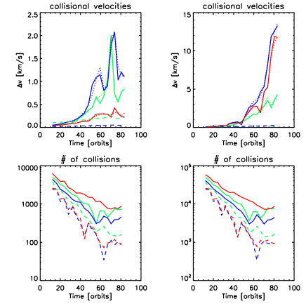
Figure 12: Average collisional velocities in the high inclination $\gamma_{F}=0.78(45^{\circ})$ case between equally (panel 1) and differently sized planetesimals (panel 2). Left panel: 10km-10km collisions (green-solid); 1km-1km collisions (blue-solid); 100m-100m collisions (red-solid). Right panel: 10km-1km (green-solid); 10km-100m (blue-solid); 1km-100m (red-solid). Threshold velocities for catastrophic disruption corresponding to the different size-combinations for the strong aggregates (dashed line) are also shown. Relative velocities have also been calculated using a larger orbit width $\Delta a=2\cdot 10^{-3}$ AU (dotted lines). Panels 3 and 4: collision count for orbital width $\Delta a=2\cdot 10^{-4}$ AU and $\Delta a=2\cdot 10^{-3}$ AU, respectively. The line colours and styles in panel 3 and 4 are as follows: green-solid (10km-10km); blue-solid (1km-1km); red-solid (100m-100m); green-dashed (10km-1km); blue-dashed (10km-100m); red-dashed (1km-100m).

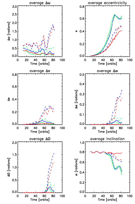
Figure 13: Average orbital parameters of the colliding planetesimal pairs in the high inclination $\gamma_{F}=45^{\circ}$ case. The line colours and styles are as follows: green-solid (10km-10km); blue-solid (1km-1km); red-solid (100m-100m); green-dashed (10km-1km); blue-dashed (10km-100m); red-dashed (1km-100m).

The orbital elements are displayed in Fig.13. We observe that the Kozai effect causes an increase of eccentricity up to $e=0.4$-0.6, such that the contribution to the relative velocity between planetesimals due to the term $\propto e_{i}\Delta\omega_{i}$ becomes large, and this is the dominant cause of high velocity collisions between equal sized bodies. The situation is different for planetesimals of different sizes. The different gas drag strengths change the relative inclination between the planetesimals and the disc, resulting in a variation of the inclination perturbations caused by disc gravity, which on the one hand causes the value of $\omega_{i}$ that is approached during the first half of the Kozai cycle to be different, and on the other hand causes the Kozai mechanism to operate on different time scales. As a result planetesimals of different sizes decouple from the disc at different times. As can be seen from panels 4 and 5 of Fig.13, the orbital planes and pericentres of different sized planetesimals become randomly distributed with $\Delta\Omega_{i}\sim 1$ and $\Delta\omega_{i}\sim 1$, and the relative velocities are increased substantially due to the terms which are proportional to $e_{i}\Delta\omega_{i}$, $\Delta\alpha_{i}$, and $\sin{(\alpha_{i})}\Delta\Omega_{i}$ in Eq. (44), with the latter term being the dominant one. As found in the low inclination case, the relative velocities of different sized planetesimals are generated due to misalignment of their pericentres $\Delta\omega_{i}$ and their orbital planes $\Delta\Omega_{i}$. In contrast to the low inclination model, however, the eccentricities, $e_{i}$, inclinations $\alpha_{i}$, and the differential nodal precession angle, $\Delta\Omega_{i}$, are much larger due to the Kozai effect, leading to very large collisional velocities.

In Fig.12 (panel 3) we display the number of collisions detected for the different size combinations, and it may be observed that the number of collisions drops to $\sim 100$ for collisions between differently sized planetesimals. As the bodies begin to orbit in different planes their encounter probability is reduced, as discussed in Sect. 5.2.1 and reported by Xie & Zhou (2009). This implies that the averaged relative velocities (panels 1 and 2) are obtained from only $\sim 10^{2}-10^{3}$ data points, and the results are in danger of becoming statistically unreliable. In order to compare these collision velocities with more statistically significant data, we also calculated the relative velocities while adopting a larger cross sectional area for the intersecting orbits corresponding to $\Delta r=2\cdot 10^{-3}$ AU. The collision probability is increased by a factor of $\sim 10$, as observed in panel 4 of Fig.12. These relative velocities are plotted as dotted lines in panels 1 and 2 of Fig. 12, and are almost indistinguishable from the data obtained with the smaller orbit width, suggesting that the results are reliable. As was discussed for the low inclination model, the reduction in the collision frequency can have potentially important consequences for planetesimal accretion, since it may favour collisions between similar sized bodies which orbit in similar planes. But, it is clear from Fig.12 that when the Kozai effect is active, large collision velocities are obtained for all size combinations.

The disruption/erosion threshold velocity for the strong aggregates is shown using the dashed lines in panels 1 and 2. The collisional velocities are substantially larger than those required for erosion or catastrophic disruption for all size combinations in this case, leading to the unsurprising conclusion that planetesimal accretion is not possible if the Kozai mechanism operates during the epoch of planet formation. For the relative velocities observed in Fig.12 of $\sim 2$km/s for equally sized planetesimals, we estimate that collisions will always lead to fragmentation unless bodies of size $\sim 10^{3}$ km have already formed.

6 Suppressing the Kozai effect

6.1 Increasing the disc mass (models 4 and 5)

The Kozai effect generates relative velocities which are always too large for collisional growth of planetesimals, at least for sizes in the range (100m-10km). An interesting question is under what conditions does the Kozai mechanism cease to operate. As discussed in Sect. 5.3 the Kozai mechanism relies on the apsidal precession induced by the binary companion halting, such that $\dot{\omega}_{i}=0$, which then allows for a secular change of the eccentricity and inclination values. If apsidal precession can be induced by another source, however, such as the disk for example, then we would expect the Kozai mechanism to be ineffective once this induced precession is fast enough (Wu & Murray 2003).

Since the apsidal precession rate caused by the disc scales with disc mass (see Eq.46), we have run simulations with an increased disc mass to see if the Kozai mechanism can be suppressed in this way. The results are shown in Fig.14 for model 4 (left panels) and 5 (right panels) with disc masses of $M_{d}=3.3\hat{M}$ and $6.6\hat{M}$, respectively, where $\hat{M}$ is the nominal disc mass used in model 3. As can be seen from the figure, the Kozai mechanism still switches on for the $M_{d}=3.3\hat{M}$ case but does not operate in the $M_{d}=6.6\hat{M}$ model. Consequently the eccentricity grows to large values in model 4, as seen in panel 1 of Fig.14, while it remains low in model 5 (panel 2).

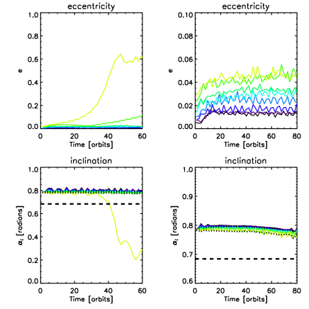
Figure 14: Orbital elements for model 4 (left panels) and model 5 (right panels). Only planetesimals with semi-major axes $a\leq 13$ AU are included. In model 4 the Kozai effect is still operating, while in model 5 it is not. Panels 1 and 2 show the eccentricity. Panels 3 and 4 display the inclination, where the short dashed lines represent the inner and outer edge of the disc and the long dashed line indicates the threshold inclination of $0.68\;(39.2^{\circ})$ above which the Kozai mechanism can operate.

6.2 Increasing binary separation (models 6 and 7)

Another way to increase the relative importance of the disc-induced apsidal precession is to decrease the gravitational influence of the binary companion. In this section we present simulations in which the separation of the binary system was increased to examine when the Kozai effect is suppressed. We consider separations of $D=90$ AU and $D=120$ AU in models 6 and 7, respectively. Because the Kozai time scale is $\propto D^{3}$, extremely long simulation times are required to prove the existence (or non existence) of the Kozai effect. The required run times would be prohibitive for a full 3D hydrodynamic simulation, so we adopted the compromise of switching off the hydrodynamic evolution of the disc in order to speed up the run times for these models. The disc in these simulations therefore remains axisymmetric and static in the precessing frame, but our adoption of a precessing reference frame causes it to precess around the binary angular momentum vector at the prescribed rate.

We tested the accuracy of this approach by re-running model 3 using a static, precessing disc model, and found similar results when compared with the run in which the disc was allowed to evolve self-consistently. Differences between the static, precessing disc model and the full hydrodynamic simulation arise mainly because the disc experiences a low amplitude nodding motion (oscillation in its inclination) with a period equal to half the binary orbit period in the full simulation (Larwood et al. 1996; Fragner & Nelson 2010), where this is driven by the time-varying gravitational field of the binary. Although the effect is relatively small, it is likely to reduce the accuracy with which a rigidly precessing disc model can be used to determine planetesimal collision velocities in detail. But, it is a useful set-up for determining the disc mass for which the Kozai mechanism operates.

The results are shown in Fig.15 for the $D=90$ AU (left panels) and $D=120$ AU model (right panels). We can observe that the Kozai effect is operating in model 6 while it is not in model 7. The time scale for the Kozai effect to increase the eccentricities is larger by a factor $3.3$, as expected, for model 6 compared to the reference model 3 due to the Kozai time scale increasing as $\sim D^{3}$. If the Kozai effect was operating in model 7, we would expect to see substantial eccentricity growth after 500 orbits (a factor 8 longer than in our reference model). This is not seen, however, and we conclude that the Kozai effect cannot operate in model 7.

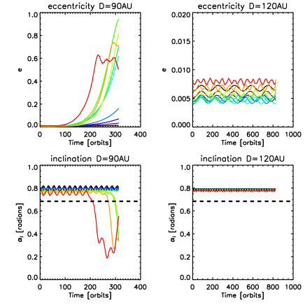
Figure 15: Orbital elements for model 6 (left panels) and model 7 (right panels). The Kozai effect is operating in model 6, but is not in model 7. The eccentricities are shown in panels 1 and 2. The inclination is shown in panels 3 and 4. The long dashed lines in panels 3 and 4 represents the $39.2^{\circ}$ inclination threshold, above which the Kozai effect can operate.

6.3 A theoretical argument

We have seen in the previous two sections that the Kozai mechanism can be suppressed provided the disc mass or the binary separation are large enough. Now we want to understand the numerical results by means of a theoretical argument. As has already been discussed, the Kozai mechanism relies on halting the apsidal precession of the planetesimals induced by the binary companion. If this can be prevented then there should be no secular net change of eccentricities or inclinations. The total net rate of apsidal precession is given by the sum of the contributions by the binary companion (Eq.54) and the disc induced apsidal precession. Since we only consider cases for which $\delta_{i}\leq\alpha_{d}$, the latter is given by Eq. (46). Hence the total apsidal precession rate experienced by a planetesimal on a circular orbit ($e_{i}=0$) is:

$$\frac{\partial\omega_{i}}{\partial t}=\frac{3\pi}{2D^{3}}\left(20a_{i}\right)^{\frac{3}{2}}\left(2-5\sin^{2}{(\omega_{i})}\sin^{2}{(\alpha_{i})}\right)-|\dot{\omega}_{D}|,$$ (60)

where $a$ and $D$ are expressed in units of AU. The first term on the right hand side of Eq. (60) accounts for the binary-induced precession, and $\dot{\omega}_{D}$ is the disc-induced precession rate given by Eq. (46). Both of these rates are expressed in time units of orbits at $a=20$ AU (the time unit used throughout the paper). In order for the Kozai mechanism to operate we require that $\frac{\partial\omega_{i}}{\partial t}=0$. This can only be true if the prograde term due to the binary companion is larger than the retrograde term of the disk. For the Kozai effect to operate, we therefore require that:

$$\frac{3\pi}{D^{3}}\left(20a_{i}\right)^{\frac{3}{2}}\geq|\dot{\omega}_{D}|.$$ (61)

Using Eq. (46), we can express this a condition on the total disc mass in terms of the planetesimal semi-major axis and binary orbit separation:

$$M_{d}\leq\frac{3\pi\hat{M}}{D^{3}}\left(20a_{i}\right)^{\frac{3}{2}}\left[C_{0}+C_{1}\left(\frac{a_{i}}{{\rm AU}}\right)+C_{2}\left(\frac{a}{{\rm AU}}\right)^{2}\right]^{-1}.$$ (62)

If this inequality is fulfilled we expect the Kozai mechanism to operate. In Fig.16 we show how the upper limit on the disc mass varies as a function of binary separation in order for the Kozai mechanism to just switch on/off for a planetesimal orbiting at a representative value of the semi-major axis $a_{i}=11$ AU, which is approximately half of the disc tidal truncation radius. The red area corresponds to the regime where the inequality is fulfilled and the Kozai-mechanism should operate. The cyan area marks the parameter space where the Kozai mechanism should not operate (large disc mass/large binary separation).

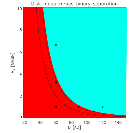
Figure 16: Plot of the parameter regime explored in the simulations. The diagram shows disc mass against binary separation, with the red area denoting the region where the Kozai mechanism should operate, and the cyan area showing the region where it should not for a planetesimal located at 11 AU. The symbols denote the outcome of the simulations, where a cross implies that the Kozai effect was switched off, and an open square indicates that the Kozai mechanism operates. The dashed and dotted line represents the same boundary for a body at $a_{i}=6$ AU and $a_{i}=15$ AU respectively.

The symbols represent the simulation results, where open squares indicate that the Kozai mechanism was found to operate (models 3, 4 and 6), while crosses represent the models in which the Kozai effect was ineffective (models 5 and 7). We see that the numerical results agree with our predictions.

We also plot the boundary lines that correspond to semi-major axes of $a_{i}=6$ AU (dashed line) and $a_{i}=15$ AU (dotted line). Between $a_{i}=6$ AU and $a_{i}=11$ AU the precession frequency due to the disc is nearly independent of semi-major axis, as can be seen from the solid line in panel 7 of Fig.1. Yet the binary precession still increases as $\propto a^{\frac{3}{2}}$. Hence the parameter space for which the Kozai mechanism operates becomes larger as the semi-major axis increases. Between $a_{i}=11$ AU and $a_{i}=15$ AU the disc precession rate increases in magnitude approximately as $\propto a_{i}^{3/2}$. Thus the boundary separating the Kozai-active versus Kozai-inactive regions does not change very much beyond $a_{i}=11$ AU.

7 Discussion and conclusions

In this paper we have investigated the dynamics of planetesimals that are embedded in a gaseous disc that is perturbed by a binary companion on a circular, inclined orbit. In contrast to previous work the planetesimals are allowed to interact with the gaseous disc via gas drag and disc gravity. The disc evolves hydrodynamically because of gravitational perturbations due to the binary companion, and the disc model we consider undergoes solid body precession around the orbital angular momentum vector of the binary system, as expected when the warp propagation time via bending waves is shorter than the differential precession time. Discs around young stars are expected to show similar behaviour since it is estimated that $\alpha<H/R$ in these systems, where $\alpha$ is the usual viscosity parameter. The key results of our study can be summarized as follows.

• In the absence of disc gravity, planetesimals undergo strong differential nodal precession, such that they eventually orbit in different planes (Marzari, Thebault & Scholl 2009; Xie & Zhou 2009). They also precess relative to the disc, so their orbits become highly inclined relative to it. We find that disc gravity acts to prevent this differential precession, and forces the planetesimals to precess with the disc on average. Viewed locally, the forcing of nodal precession by the binary companion causes the planetesimals to oscillate about the midplane of the disc, with an amplitude that depends on the size of the planetesimals because of the influence of gas drag in damping this relative motion. This key result suggests that the influence of the gravitational field of the precessing disc should always be included in future studies of planet formation in inclined binary systems.

• Previous studies that focused on the influence of a coplanar, eccentric binary companion have shown that the eccentric binary generates a forced eccentricity in the planetesimal swarm. Gas drag acts to align the pericentres of planetesimals which are of the same size, such that collisions between same-sized bodies are dominated by keplerian shear. Collisions between different sized bodies occur with higher velocity due to the misaligned orbits (Marzari & Scholl 2000; Thebault, Marzari & Scholl 2006). We find that for a circular binary, where the eccentricity of planetesimals is largely generated by high frequency terms in the disturbing function, strong alignment of pericentres is not observed.

• Previous work which has examined planetesimal dynamics in modestly inclined and eccentric binary systems suggests that gas drag causes size-dependent phasing of both pericentres and the lines of nodes of perturbed planetesimals (Xie & Zhou 2009). This has the effect of favouring collisions between same sized objects, for which the collision velocity is dominated by the keplerian shear, and as such it has been suggested that this may provide an effective channel for planetesimal growth in inclined binary systems. Our results obtained for a binary with inclination $\gamma_{F}=25^{\circ}$ are in basic agreement with this, as we find that same-sized planetesimals do indeed occupy very similar orbital planes, whereas the orbits of differently sized bodies are mutually inclined. This arises in our case because of the different amplitudes of oscillation about the disc midplane observed for planetesimals of different size, with smaller bodies remaining closer to the midplane. We thus find that the collision velocities between differently sized bodies are significantly larger than between same-sized bodies (typically $v_{coll}\simeq 200$ ms^-1 for different sized objects and $v_{coll}\simeq 50$ - 70 ms^-1 for same-sized objects). We note that the lack of pericentre alignment observed in our simulations leads to the substantial collision velocities between same size bodies. Collisions with the velocities described above are likely to be erosive or disruptive, depending on the mass ratio of the colliding bodies.

• For highly inclined systems with $\gamma_{F}=45^{\circ}$, we find that the Kozai mechanism can operate, causing large changes in the eccentricities and inclinations of the planetesimals, and leading to collisional velocities that are much too large to allow for planetesimal accretion. The long term influence of the disc in cases where the Kozai mechanism operates is to modify the period associated with the Kozai cycle by periodically forcing the planetesimal inclinations to fall below, or rise above, the critical value for the Kozai effect to operate, $\alpha_{K}=39.2^{\circ}$. We find that planetesimals of size 10m - 10km all experience the Kozai effect.

• Increasing the disc mass or binary separation can suppress the Kozai effect, as disc gravity can induce apsidal precession which is fast enough to render the Kozai mechanism ineffective. For a binary separation of $D=60$ AU, and disc truncation radius of 20 AU, we find that we need to increase the disc mass by a factor of $\sim 6$ above the minimum mass solar nebula (MMSN) value in order to switch off the Kozai effect at a representative orbital radius of $a_{i}=11$ AU. Increasing the binary separation to $D=120$ AU, and maintaining the mass of our disc at its nominal value (equivalent to the MMSN) also rendered the Kozai mechanism inoperative.

In the light of the above findings, we can conclude that highly inclined, distant binary companions probably will not induce the Kozai effect during planet formation while the disc is present, although it may do so once the disc has dissipated, such that the final planetary system is strongly perturbed. But we note that the peak in the distribution of binary orbit separations occurs at $D\simeq 30$ AU (Duquennoy & Mayor 1991; Ghez et al. 1993; Leinert et al. 1993), which is small enough for the Kozai mechanism to operate during the planet formation epoch when the gas disc is present. There are number of extrasolar planetary systems, however, which are observed to be in relatively close binary systems, $\gamma$ Cephei being a notable example (see Kley & Nelson 2008, and references therein). Here the binary separation is only a few tens of AU, such that the Kozai mechanism could possibly have operated when planetesimals were accreting. The fact that a planet is observed in this system with a modest orbital eccentricity is probably an indication that the binary inclination is too small to allow the Kozai mechanism to operate. This is consistent with the findings of Hale (1994) that binary orbits with $D<40$ AU tend to be reasonably well aligned with the stellar spin axes.

A key issue that needs to be addressed in the future is the evolution of a planetesimal swarm in a binary system where the orbit is both inclined and eccentric. Our results suggest that a circular binary system does not allow for the pericentres of perturbed planetesimals to be well aligned, since a circular orbit is unable to impose a preferred direction on the system, and this is in clear contrast to studies which have considered an eccentric companion. It should be noted, however, that the inclusion of the disc gravity will be of crucial importance in such a study, since it will significantly perturb the orbits of the planetesimals. This is particularly the case when the planetesimal orbits are inclined relative to the disc midplane, and the presence of an eccentric binary companion may also cause the disc itself to become eccentric (Kley & Nelson 2008; Kley et al. 2008) (where the disc eccentricity may be dependent on the disc self-gravity (Marzari et al. 2009)), further complicating matters. We further note that the inner edge of our computational domain was located at $R=2$ AU, so our present study examines planet formation in the region normally associated with giant planet formation. Studies of this type which examine terrestrial planet formation closer to the central star will require deployment of substantially more powerful computational resources than were used here, in order to simulate the larger range of time scales in the problem. Such a study should also include a more realistic planetesimal size distribution so that the possibilty of accretion occuring via collisions between similarly sized bodies can be explored.

In this paper we have only considered planet formation via collisions between planetesimals, whereas dust accumulation onto individual planetesimals could still lead to planetary growth as long as collisions between planetesimals can be avoided. This issue has been recently been addressed by Paardekooper & Leinhardt (2010); Xie et al. (2010), where they show that km-sized planetesimals may grow in size by two orders of magnitude due to accretion of collisional debris if the efficiency of planetesimal formation stays low, i.e. only a few planetesimals form. This study involved two-dimensional simulations, and it will be interesting to examine how the results change for a misaligned system where planetesimals may orbit out of the disc midplane where the majority of the dust and collisional debris will reside. As we have seen in Sect. 5.2, 10 km sized planetesimals tend to have orbits which are inclined relative to the disc by more that the disc scale height, once their free particle rates are substantially different from the disc precession rate. Planetesimal formation via dust accretion is therefore only expected in radial regions of the disc where the precession rate of the planetesimals and the disc are well-matched. Closer to the inner or outer edge of the disc, efficient dust accretion may not be possible due to the large relative inclinations of the planetesimals. This, and other issues discussed in this paper, will be the subject of future publications.