Mean-field solar dynamo models with strong meridional flow at the bottom of the convection zone
Abstract
The paper presents a study of kinematic axisymmetric mean-field dynamo models for a case of the meridional circulation with a deep-seated stagnation point and a strong return flow at the bottom of the convection zone. This kind of circulation follows from mean-field models of the angular momentum balance in the solar convection zone. We show that it is possible for this types of meridional circulation to construct kinematic dynamo models that resemble in some aspects the sunspot magnetic activity cycle. The dynamo model includes turbulent sources of the large-scale poloidal magnetic field production, due to kinetic helicity and a combined effect due to Coriolis force and the large-scale current. In these models the toroidal magnetic field, which is responsible for the sunspot production, is concentrated at the bottom of the convection zone, and is transported to low-latitude regions by the meridional flow. The meridional component of the poloidal field is also concentrated at the bottom of the convection zone while the radial component is concentrated in near polar regions. There are some issues which, perhaps, are resulted from the given meridional circulation pattern and the distribution of the magnetic diffusivity inside convection zone. In particular, in the near-equatorial regions the phase relations between the toroidal and poloidal components disagree with observations. Also, we show that the period of the magnetic cycle may not always monotonically decrease with the increase of the meridional flow speed. Thus, for the further progress it is important to determine the structure of the meridional circulation, which is one of the critical properties, from helioseismology observations.
1 Introduction
The widely accepted paradigm about the nature of the global magnetic activity of the Sun assumes that meridional circulation is an important part of the dynamo processes operating in the solar convection zone (Choudhuri et al., 1995; Durney, 1995; Choudhuri & Dikpati, 1999; Miesch et al., 2010). The current flux-transport and mean-field dynamo models, (e.g., Dikpati & Charbonneau, 1999; Guerrero & Muñoz, 2004; Bonanno et al., 2002), typically employ an analytical profile of the meridional circulation pattern, which has to satisfy a mass conservation equation and the relevant boundary conditions. One of the basic features of this profile is that the circulation stagnation point is close to the middle of the convection zone, (e.g., Bonanno et al., 2002; Dikpati et al., 2004). However, such ad hoc models of the meridional flow have no support from the mean-field theory of the angular momentum distribution in the solar convection zone (Kitchatinov & Rüdiger, 1999; Kitchatinov & Olemskoy, 2011), also see, Garaud & Acevedo Arreguin (2009). The theory predicts the meridional circulation pattern with nearly equal amplitudes of the flow velocity at the bottom and top of the convection zone. The stagnation point of this flow is close to the bottom of convection zone, near , and the circulation is concentrated near the convection zone boundaries. Rempel(2005; 2006) obtained a similar meridional circulation profile with a deep stagnation point and used it to construct a nonlinear dynamo model.
The physical mechanisms of the strong deviation of the meridional circulation pattern from the simple analytical models are discussed in the recent paper by Kitchatinov & Olemskoy (2011). Here, we briefly summarize their main arguments. The distribution of large-scale flows in the balk of convection zone is close to the Taylor-Proudman balance. However, this balance is violated near the boundaries. This results in a concentration of the velocity circulation in the Eckman layers near the bottom and the top of convection zone (Durney, 1999; Miesch et al., 2006; Brun et al., 2010).
Our goal is to investigate how the meridional circulation with a fast return flow at the bottom of the convection zone can affect solar dynamo models. We construct a series of kinematic mean-field dynamo models that employ the meridional circulation pattern suggested by Kitchatinov & Olemskoy (2011). These dynamo models include the turbulent generation of the magnetic field due to the kinetic helicity ( -effect), the combined effect of the Coriolis force and large-scale current (-effect), and the toroidal magnetic field generation due to the differential rotation (-effect). Following Krause and Rädler(1980) these models can be classified as dynamo. Our approach is to investigate conditions of the dynamo instability for this type of the meridional circulation and determine the basic properties of the dynamo solution at the instability threshold. This is a kinematic dynamo problem. The next section describes the formulation of the mean-field dynamo model, including the basic assumptions, the reference model of the solar convection zone, and input parameters of the large-scale flows. Section 3 presents the results and discussion. The main findings are summarized in Section 4.
2 Basic equations
2.1 Formulation of model
The dynamo model is based on the standard mean-field induction equation in perfect conductive media (Krause and Rädler, 1980):
| (1) |
where is the mean electromotive force, with being the turbulent fluctuating velocity and magnetic field respectively; is the mean velocity. General expression for was computed by Pipin (2008)(hereafter P08). Following Krause and Rädler(1980) we write the expression for the mean-electromotive force as follows:
| (2) |
where, tensor represents the turbulent alpha effect, tensor describes the turbulent pumping, and the term describes the anisotropic diffusion due to the Coriolis force and the effect (Rädler, 1969).
We consider a large-scale axisymmetric magnetic field, , where is the azimuthal component of the magnetic field, is proportional to the azimuthal component of the vector potential, is radial coordinate and - polar angle. The mean flow is given by velocity vector , where is the angular velocity of the solar differential rotation and , , represent velocity components of the meridional circulation. The mean-field magnetic field evolution of is governed by the dynamo equations, which follow from Eq.(1):
| (3) | |||||
| (4) |
We introduce the free parameter to control the turbulent diffusion coefficient (see Appendix). A solar-type dynamo model can be constructed not only with the -effect as a prime turbulent source of the poloidal magnetic field generation (Stix, 1976; Pipin & Seehafer, 2009; Seehafer & Pipin, 2009). The exact mechanism of the large-scale poloidal magnetic field production on the Sun is not known. After Parker (1955), it is belived that the -effect (associated with cyclonic convection) is the most important turbulent source of the poloidal magnetic field generation on the Sun. The -effect particularly important role for the dynamo because it describes a leading term of the Taylor expansion of the turbulent mean-electromotive force in terms of the scale separation parameter. In addition, the mean-field theory predicts the magnetic field generation effects due to the interaction of the Coriolis force (-effect) and the differential rotation (-effect, where is the large-scale velocity shear) with large-scale electric current (see, Rädler, 1969; Krause & Rädler, 1980; Rogachevskii & Kleeorin, 2003). The role of these mechanisms for the solar dynamo is not well understood though it was shown (Pipin & Seehafer, 2008, 2009) that it is possible to construct the solar-type dynamo models including these effects. Our model includes the - and effects. We introduce free parameters and to control their strength.
We use the solar convection zone model computed by Stix (2002), in which mixing length , where is the inverse pressure scale height, and . We confine the integration domain between 0.712 and 0.972 in radius. It extends from the pole to pole in latitude. The differential rotation profile, , , is a modified version of the analytical approximation to helioseismology data proposed by Antia et al. (1998), see Figure 1a.
a)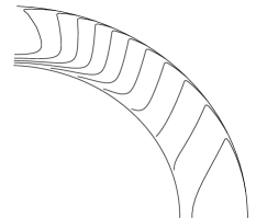 b)
b)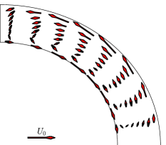 c)
c)
d)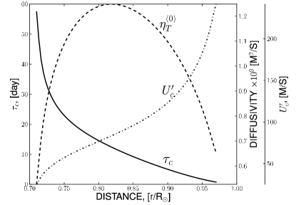 e)
e)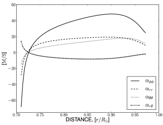
The meridional flow is modeled in the form of two stationary circulation cells, one in the northern and one in the southern hemisphere, with a poleward motion in the upper and equator-ward motion in the lower part of the convection zone. Following Kitchatinov & Olemskoy (2011), the meridional circulation velocity components were approximated via the orthogonal Chebyshev polynomial decompositions:
| (5) | |||||
| (6) |
where
| (7) |
Here, are the radial boundaries of the integration domain. In our case, and . The coefficients , are given in Table 1. Parameter controls the speed of the meridional circulation. Kitchatinov & Olemskoy (2011) obtain .
| n | 0 | 1 | 2 | 3 |
|---|---|---|---|---|
| -0.13432(5) | - 0.40473(6) | - 0.02170(3) | - 0.10718(5) | |
| - 0.0681469(4) | - 0.006839(4) | -0.032516(1) | - 0.0027(4) |
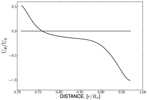
The geometry of the meridional flow is illustrated in Figure 1(b). Figure 1(c) shows the latitudinal component of the circulation in units .
The boundary conditions represent a perfect conductor at the bottom and the potential magnetic field configuration outside the domain.
2.2 Method of solution
We investigate the linear stability of the dynamo equations (3,4) and determine unstable dynamo modes. Then we construct linear dynamo solutions using the corresponding eigen-functions. Our approach to solve the linear problem was described in details by Pipin & Seehafer (2009) and Seehafer & Pipin (2009). We use a Galerkin method, expanding the magnetic field in terms of a basis that satisfies the boundary conditions (Boyd, 2001; Livermore & Jackson, 2005). The system of Eqs. (3) and (4) has exponentially growing or decaying solutions, which we represent in the form
| (8) | |||||
| (9) |
where and are linear combinations of Legendre polynomials, and is the associated Legendre function of degree and order . These expansions ensure the regularity of the solutions at the poles and . The integrations in radius and latitude, which are needed for calculating the expansion coefficients and , were done by means of the Gauss-Legendre procedure. The eigenvalue problem for determining the eigenvalues, , and the associated eigenfunctions was solved by using the LAPACK software. There are two types of dynamo eigenmodes: 1) modes with a symmetric distribution of the toroidal component and antisymmetric distribution of the poloidal component , relative to the equator, called here “S-modes”, and 2) vice-versa antisymmetric al modes, called “A-modes”. We define the eigenvalues of the S- and A-modes as and . The spectral resolution of our calculations was 16 radial and 25 latitudinal basis functions. The results were qualitatively confirmed by a number of runs with larger number of the basis functions.
3 Results
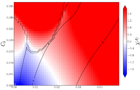
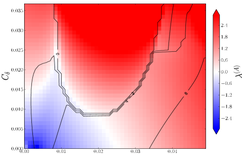
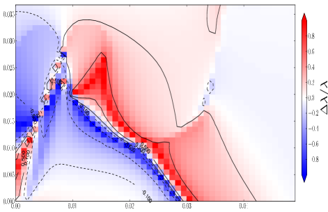
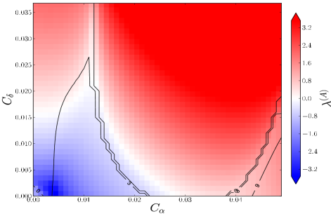
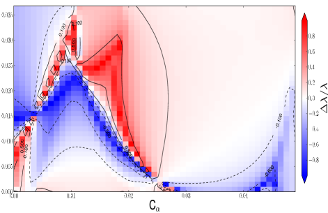
We calculate the dynamo solutions for a low level of the background turbulent diffusivity, choosing , in order to approximately match the period of the eigenmodes with the solar cycle period. This corresponds to the background diffusivity . Figure 2 (left column) shows the linear-stability diagrams for the dynamo models with the meridional circulation speed values equal to and . The growth rate of the first, most unstable dynamo mode (A-mode) is shown by the color-scale plots in the plane, where and are the free parameters that control the strength of the and effects. We find that the dynamo instability region (represented by red color) changes significantly with the increase of the meridional circulation speed. For the slow meridional circulation it is found that the first A-mode is stable and steady in the absence of the -effect (). It has the excitation threshold of . In the opposite limit, when , the first mode is stable and oscillating. Its oscillation frequency grows with the increase of the -effect parameter . The excitation threshold is . The oscillation frequency of the mode at the threshold is about .
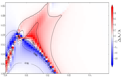
The right column in Figure 2 shows the growth rate of the first A-mode relative to the first S-mode. The relative difference is characterized by parameter . This helps to identify the regions in the parameter space where the A-mode dominates the S-mode. We find that in the case of the A-mode is dominant for . In this regime we look for a solar-type dynamo solution, because in the solar dynamo the toroidal magnetic field is A-type (antisymmetric relative to the equator).
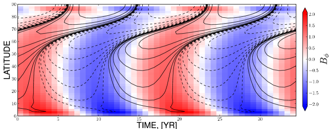
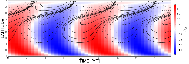
For an example, we examine the case of , when the first A-mode has the frequency . Figure 3 shows the snapshots of the magnetic field variation inside the convection zone (top) and the time-latitude “butterfly” diagram for this mode (bottom). The snapshots show that the toroidal magnetic field is concentrated at the bottom of the convection zone, and the poloidal field is concentrated in the polar regions. Also, the toroidal magnetic field is globally distributed in the bulk of the convection zone. The maximum of the toroidal field distribution drifts to the equator at the bottom of the convection zone and moves to the pole near the surface. The bottom panel of Figure 3 shows the butterfly diagrams of the toroidal field at the bottom of the convection zone (color background) and for the radial magnetic fields at the surface (contour lines). The toroidal magnetic field evolution pattern has the polar and equatorial branches. The equatorial branch is strongly concentrated to equator. The phase relation between the radial magnetic field in the polar regions and the toroidal field in the equatorial regions is in agreement with observations of the polar magnetic field and the sunspot butterfly diagram, assuming that sunspots are formed by emerging toroidal magnetic field. However, this dynamo mode lacks the equatorial branch of the large-scale radial magnetic field, which is also found in observations. The period of the dynamo period is about 12 years. This is as twice as short compared to the solar magnetic cycle. The period can be increased by further decreasing the diffusivity parameter by a factor of 2 (). However, this leads to decrease of the excitation threshold and increase of the effective magnetic Reynolds number (). This means that the S-mode becomes dominant, and solution no longer corresponds to the solar dynamo. Figure 2 shows that for the case of the S-mode dominates.

Inspecting the results in Figure 3 we can conclude that the increase of the meridional circulation speed has two main effects on the dynamo instability. Firstly, the larger the larger the unstable area in the space, occupied by the first unstable A-mode (associated with a non-oscillating dynamo solution). Secondly, the S-mode becomes dominant near the instability threshold everywhere, both for the case of and arbitrary and for the case of arbitrary and . The combination of the and effects can make the A-mode dominant, but it represents a non-oscillating dynamo solution.
In another example, we examine the model, when the poloidal field is generated both by the -effect and the -effect, e.g., and . The oscillation frequency of the first unstable A-mode is about . Near the excitation threshold, the A-mode is highly dominant over the first S-mode. Figure 4 shows the snapshots of the magnetic field variations inside the convection zone (top) and the butterfly diagram for this mode(bottom). The snapshots of the magnetic field evolution inside the convection zone are similar to the previous case. However, the toroidal magnetic field is stronger concentrated at the bottom of convection zone, and the polar branch of the toroidal magnetic field evolution near is weaker near the surface. The period of dynamo wave is about 24 years, close to the solar cycle. Generally, we see a significantly better agreement with the observations than in the previous case.

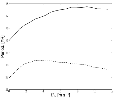
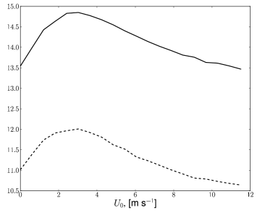
In Figure 5 the dependence of the dynamo wave period on the speed of the meridional flow along the stability threshold shown. Contrary to previous results, e.g., (Bonanno et al., 2002; Seehafer & Pipin, 2009) the period is not a monotonic function of the flow velocity. The main reason is that here we use the meridional circulation with a different depth dependence. We made a check how the presented results may depend on the distribution of the alpha effect. For this,, we switched off the effects of the turbulent mixing stratification, in Eq.(6). The dynamo period as a function of the meridional flow speed for this case is shown in Figure 5(right). We find that dependence of the dynamo period on the flow speed is much stronger in case for both types of dynamo.
4 Discussion and conclusions
We have studied kinematic axisymmetric mean-field dynamo models for a meridional circulation pattern with a deep seated stagnation point. This kind of circulation is suggested by the mean-field models of the angular momentum balance in the solar convection zone. We show that by adjusting the turbulent sources of the poloidal magnetic field generation and the turbulent diffusion strength it is possible to construct a mean-field dynamo model that resembles in some aspects the solar magnetic cycle. The most important features of the investigated models are the following.
The maximum strength of the toroidal magnetic field, which is believed to be responsible for the sunspots production, is concentrated near the bottom of the convection zone. This field is transported to the equatorial regions by the meridional flow. The meridional component of the poloidal field is also concentrated at the bottom of the convection zone. The large-scale radial field is concentrated near the poles. It reverses sign when the maximum of the toroidal field gets close to equator. This is not quite consistent with the solar observations, which show that the polar field reversals happen earlier in the cycle. Similar result was demonstrated in the kinematic flux-transport model by Rempel (2006). His model had a qualitatively similar meridional circulation pattern, and the speed at the bottom of the convection zone was as twice as slow compared to our case. We believe that this feature (the phase relation) is inherent for this type of the meridional flow, which produced conveyor-belt like circulation of magnetic field (Dikpati et al., 2004). The equatorward and poleward conveyor bands are not well connected in our case because circulation is quite weak in the bulk of convection zone.
We find that including the combined action of the and effects for the poloidal magnetic field generation improve the agreement of the model with observation. Contrary to the usual expectations that come from the results of the flux-transport dynamo model we find that the period of the dynamo cycle does not always become shorter when the speed of the meridional circulation increases. In our model this rule works for the amplitude of flow in the case of the dynamo with the effect dependent on the density stratification, and for in the case of the with the effect dependent on both the density and the turbulent diffusivity stratifications. The dependence of the dynamo period on the flow amplitude is much stronger if the alpha effect does not depend on the turbulence intensity stratification, .
Thus, by measuring the distributions of the magnetic activity and meridional circulation characteristics on the Sun and possibly other cool stars we may get indirect information about contribution of the effect to the dynamo and the relative contributions to the effect due to density and the turbulent diffusivity stratifications as well.
We conclude that the meridional flow pattern and speed have to be considered among the most important constrains on the stellar dynamo. Our results show the possibility of using helioseismic observations of the meridional circulation for the diagnostic purpose of the solar dynamo, because the dynamo properties significantly depends on the depth of the flow stagnation point.
5 Acknowledgements
This work was supported by NASA LWS NNX09AJ85G grant and partially by RFBR grant 10-02-00148-a.
References
- Antia et al. (1998) Antia, H. M., Basu, S., & Chitre, S. M. 1998, MNRAS, 298, 543
- Bonanno et al. (2002) Bonanno, A., Elstner, D., Rüdiger, G., & Belvedere, G. 2002, A&A, 390, 673
- Boyd (2001) Boyd, J. 2001, Chebyshev and Fourier Spectram Methods, second edition edn. (Dover, New York), 688
- Brandenburg & Subramanian (2005) Brandenburg, A., & Subramanian, K. 2005, Phys. Rep., 417, 1
- Brun et al. (2010) Brun, A. S., Antia, H. M., & Chitre, S. M. 2010, A&A, 510, A33+
- Choudhuri & Dikpati (1999) Choudhuri, A. R., & Dikpati, M. 1999, Sol. Phys., 184, 61
- Choudhuri et al. (1995) Choudhuri, A. R., Schussler, M., & Dikpati, M. 1995, A&A, 303, L29+
- Dikpati & Charbonneau (1999) Dikpati, M., & Charbonneau, P. 1999, ApJ, 518, 508
- Dikpati et al. (2004) Dikpati, M., de Toma, G., Gilman, P. A., Arge, C. N., & White, O. R. 2004, ApJ, 601, 1136
- Durney (1995) Durney, B. R. 1995, Sol. Phys., 160, 213
- Durney (1999) Durney, B. R. 1999, ApJ, 511, 945
- Frisch et al. (1975) Frisch, U., Pouquet, A., Léorat, J., & A., M. 1975, J. Fluid Mech., 68, 769
- Garaud & Acevedo Arreguin (2009) Garaud, P., & Acevedo Arreguin, L. 2009, ApJ, 704, 1
- Guerrero & Muñoz (2004) Guerrero, G. A., & Muñoz, J. D. 2004, MNRAS, 350, 317
- Kitchatinov & Olemskoy (2011) Kitchatinov, L. L., & Olemskoy, S. V. 2011, MNRAS, 411, 1059
- Kitchatinov & Rüdiger (1999) Kitchatinov, L. L., & Rüdiger, G. 1999, A&A, 344, 911
- Kleeorin et al. (1996) Kleeorin, N., Mond, M., & Rogachevskii, I. 1996, A&A, 307, 293
- Krause & Rädler (1980) Krause, F., & Rädler, K.-H. 1980, Mean-Field Magnetohydrodynamics and Dynamo Theory (Berlin: Akademie-Verlag)
- Livermore & Jackson (2005) Livermore, P. W., & Jackson, A. 2005, Geophysical and Astrophysical Fluid Dynamics, 99, 467
- Miesch et al. (2010) Miesch, M. S., Brown, B. P., Browning, M. K., Brun, A. S., & Toomre, J. 2010, ArXiv e-prints
- Miesch et al. (2006) Miesch, M. S., Brun, A. S., & Toomre, J. 2006, ApJ, 641, 618
- Moffatt (1978) Moffatt, H. K. 1978, Magnetic Field Generation in Electrically Conducting Fluids (Cambridge, England: Cambridge University Press)
- Parker (1955) Parker, E. N. 1955, ApJ, 122, 293
- Pipin (2008) Pipin, V. V. 2008, Geophysical and Astrophysical Fluid Dynamics, 102, 21
- Pipin & Seehafer (2008) Pipin, V. V., & Seehafer, N. 2008, ArXiv e-prints
- Pipin & Seehafer (2009) Pipin, V. V., & Seehafer, N. 2009, A&A, 493, 819
- Rädler (1969) Rädler, K.-H. 1969, Monats. Dt. Akad. Wiss., 11, 194
- Rempel (2005) Rempel, M. 2005, ApJ, 622, 1320
- Rempel (2006) Rempel, M. 2006, ApJ, 647, 662
- Rogachevskii & Kleeorin (2003) Rogachevskii, I., & Kleeorin, N. 2003, Phys. Rev.E, 68, 1
- Seehafer & Pipin (2009) Seehafer, N., & Pipin, V. V. 2009, A&A, 508, 9
- Stix (1976) Stix, M. 1976, Astron. Astrophys., 47, 243
- Stix (2002) Stix, M. 2002, The Sun. An Introduction (Springer)
- Vainshtein & Kitchatinov (1983) Vainshtein, S. I., & Kitchatinov, L. L. 1983, Geophys. Astrophys. Fluid Dynam., 24, 273
6 Appendix
Here we describe the components of the mean-electromotive force which is used in the model. The tensor represents the turbulent alpha effect, and in accordance with P08 it is given by
tensor describes the turbulent pumping
| (11) |
and the term describes the anisotropic diffusion due to the Coriolis force and the effect (Rädler, 1969),
| (12) |
functions (given below) depend on the Coriolis number and the typical convective turnover time in the mixing-length approximation is . The turbulent diffusivity is parametrized in the form, , where is the characteristic mixing-length turbulent diffusivity, is the RMS convective velocity, is the mixing length, is a constant to control the intensity of turbulent mixing. The background turbulence is a state of turbulent flows in the absence of the mean magnetic fields and global rotation. The others quantities in Eqs.(6,11,12) are: is the density stratification scale, is the scale of turbulent diffusivity, is a unit vector along the axis of rotation. Equations (6,11,12) take into account the influence of the fluctuating small-scale magnetic fields, which can be present in the background turbulence (see discussions in Frisch et al., 1975; Moffatt, 1978; Vainshtein & Kitchatinov, 1983; Kleeorin et al., 1996; Brandenburg & Subramanian, 2005). In our paper, the parameter , which measures the ratio between the magnetic and kinetic energies of fluctuations in the background turbulence, is assumed equal to 1. This corresponds to the energy equipartition.
Below we give the functions of the Coriolis number defining the dependence of the turbulent transport generation and diffusivities on the angular velocity: