Multi-Hop Routing and Scheduling in Wireless Networks in the SINR Model

Abstract

We present an algorithm for multi-hop routing and scheduling of requests in wireless networks in the sinr model. The goal of our algorithm is to maximize the throughput or maximize the minimum ratio between the flow and the demand.

Our algorithm partitions the links into buckets. Every bucket consists of a set of links that have nearly equivalent reception powers. We denote the number of nonempty buckets by $\sigma$. Our algorithm obtains an approximation ratio of $O(\sigma\cdot\log n)$, where $n$ denotes the number of nodes. For the case of linear powers $\sigma=1$, hence the approximation ratio of the algorithm is $O(\log n)$. This is the first practical approximation algorithm for linear powers with an approximation ratio that depends only on $n$ (and not on the max-to-min distance ratio).

If the transmission power of each link is part of the input (and arbitrary), then $\sigma=O(\log\Gamma+\log\Delta)$, where $\Gamma$ denotes the ratio of the max-to-min power, and $\Delta$ denotes the ratio of the max-to-min distance. Hence, the approximation ratio is $O(\log n\cdot(\log\Gamma+\log\Delta))$.

Finally, we consider the case that the algorithm needs to assign powers to each link in a range $[P_{\min},P_{\max}]$. An extension of the algorithm to this case achieves an approximation ratio of $O[(\log n+\log\log\Gamma)\cdot(\log\Gamma+\log\Delta)]$.

1 Introduction

In this paper we deal with the problem of maximizing throughput in a wireless network. Throughput is a major performance criterion in many applications, including: file transfer and video streaming. It has been acknowledged that efficient utilization of network resources requires so called cross layered algorithms [LSS06]. This means that the algorithm deals with tasks that customarily belong to different layers of the network. These tasks include: routing, scheduling, management of queues in the nodes, congestion control, and flow control.

The problem we consider is formulated as follows. We are given a set $V$ of $n$ nodes in the plane. A link $e$ is a pair $(s_{e},r_{e})$ of nodes with a power assignment $P_{e}$. The node $s_{e}$ is the transmitter and the node $r_{e}$ is the receiver. In the sinr model, $r_{e}$ receives a signal from $s_{e}$ with power $S_{e}=P_{e}/d_{e}^{\alpha}$, where $d_{e}$ is the distance between $s_{e}$, and $r_{e}$ and $\alpha$ is the path loss exponent. The network is given a set of requests $\{R_{i}\}_{i=1}^{k}$. Each request is a $3$-tuple $R_{i}=({\hat{s}}_{i},{\hat{t}}_{i},b_{i})$, where ${\hat{s}}_{i}\in V$ is the source, ${\hat{t}}_{i}\in V$ is the destination, and $b_{i}$ is the requested packet rate. The output is a multi-commodity flow $f=(f_{1},\ldots,f_{k})$ and an sinr-schedule $S=\{L_{t}\}_{t=0}^{T-1}$ that supports $f$. Each $L_{t}$ is a subset of links that can transmit simultaneously (sinr-feasible). The goal is to maximize the total flow $|f|=\sum_{i=1}^{k}|f_{i}|$. We also consider a version that maximizes $\min_{i=1\ldots k}|f_{i}|/b_{i}$. Let $\Delta\triangleq{d_{\max}}/d_{\min}$ is the ratio between the maximum and minimum length of a link, and $\Gamma\triangleq P_{\max}/P_{\min}$ the ratio between the maximum and minimum transmission power. For the case in which $\max_{e\neq e^{\prime}}\frac{S_{e}}{S_{e^{\prime}}}=O(1)$, the approximation ratio achieved by the algorithm is $O(\log n)$. For arbitrary powers and link lengths, the approximation ratio achieved by the algorithm is $O(\log n\cdot(\log\Gamma+\log\Delta))$.

Previous Work.

Gupta and Kumar [GK00] studied the capacity of wireless networks in the sinr-model and the graph model for random instances in a square. The sinr-model for wireless networks was popularized in the algorithmic community by Moscibroda and Wattenhofer  [MW06]. NP-Completeness for scheduling a set of links was proven by Goussevskaia [GOW07].

Algorithms for routing and scheduling in the sinr-model can be categorized by four main criteria: maximum capacity with one round vs. scheduling, multi-hop vs. single-hop, throughput maximization vs. latency minimization, and the choice of transmitter powers. In the single-hop setting, routing is not an issue, and the focus is on scheduling. If the objective is latency minimization, then each request is treated as a task, and the goal is to minimize the makespan.

The following problems are considered. (1) cap-1slot: find a subset of maximum cardinality that is SINR-feasible. (2) lat-1hop: find a shortest SINR-schedule for a set of links. (3) lat-paths: find a shortest SINR-schedule for a set of paths. (4) lat-route: find a routing and a shortest SINR-schedule for a set of multi-hop requests. (5) throughput-route: find a routing and maximum throughput SINR-schedule for a set of multi-hop requests. We briefly review some of the algorithmic results in this area published in the last three years.

Chafekar et al. [CKM⁺07] present an approximation algorithm for lat-route. The approximation ratio is $O(\log n\cdot\log\Delta\cdot\log^{2}\Gamma)$. Fanghänel et al. [FKV10] improved this result to $O(\log\Delta\cdot\log^{2}n)$. Goussevskaia et al. [GWHW09] pointed out that $\log\Delta$ can be $\Omega(n)$, and presented the first approximation algorithm whose approximation ratio is always nontrivial. In fact, the approximation ratio obtained by Goussevskaia et al. [GWHW09] is $O(\log n)$ for the case lat-1hop with uniform power transmissions.

Halldorsson [Hal09] presented algorithms for lat-1hop with mean power assignments. He presented an $O(\log n\log\log\Delta)$-approximation and an $O(\log\Delta)$-online algorithm that uses mean power assignments with respect to OPT that can choose arbitrary power assignments (see also [Ton10]).

Halldorsson and Mitra [HM11a] presented a constant approximation algorithm for cap-1slot problem with uniform, linear and mean power assignments. In addition, by using the mean power assignment, the algorithm obtains a $O(\log n+\log\log\Delta)$-approximation with respect to arbitrary power assignments.

Kesselheim and Vöcking  [KV10] give a distributed randomized algorithm for lat-1hop that obtains an $O(\log^{2}n)$-approximation using uniform and linear powers. Halldorson and Mitra  [HM11b] improve the analysis to achieve an $O(\log n)$-approximation.

Kesselheim [Kes11] presents approximation results in the sinr-model: an $O(1)$-approximation for cap-1slot, an $O(\log n)$-approximation for lat-1hop, an $O(\log^{2}n)$-approximation for lat-paths and lat-route. In  [Kes11] there is no limitation on power assignment imposed neither on the solution nor on the optimal solution. In practice, power assignments are limited, especially for mobile users with limited power supply.

The most relevant work to our result is by Chafekar et al. [CKM⁺08] who presented approximation algorithms for throughput-route. They present the following results, an $O(\log\Delta)$-approximation for uniform power assignment and linear power assignment, and an $O(\log\Gamma\cdot\log\Delta)$ for arbitrary power assignments.

For linear powers, Wan et al. [WFJ⁺11] obtain a $O(\log n)$-approximation for throughput-route. The algorithm is based on a reduction to the single-slot problem using the ellipsoid method. In [Wan09], Wan writes that “this algorithm is of theoretical interest only, but practically quite infeasible.” For the case that the algorithm assigns powers from a limited range, Wan et al. [WFJ⁺11] achieve an $O(\log n\cdot\log\Gamma)$-approximation ratio.

Our result.

We present an algorithm for throughput-route. Our algorithm partitions the links into buckets. Every bucket consists of a set of links that have nearly equivalent reception powers. We denote the number of nonempty buckets (also called the signal diversity of the links) by $\sigma$. Our algorithm obtains an approximation ratio of $O(\sigma\cdot\log n)$, where $n$ denotes the number of nodes.

For the case of linear power assignment the signal diversity is $\sigma=1$, hence the approximation ratio of the algorithm is $O(\log n)$. This is the first practical approximation algorithm for linear powers that obtains an approximation ratio that depends only on $n$ (and not on ratio of the max-to-min distance). This improves the $O(\log\Delta)$-approximation of Chafekar et al. [CKM⁺08] for linear power assignment. As pointed out in [GWHW09], $\log\Delta$ can be $\Omega(n)$. The linear power assignment model makes a lot of sense since it implies that, in absence of interferences, transmission powers are adjusted so that the reception powers are uniform.

In the case of arbitrary given powers, the signal diversity is $\sigma=O(\log\Gamma+\log\Delta)$. Hence, the approximation ratio is $O(\log n\cdot(\log\Gamma+\log\Delta))$. For arbitrary power assignments Chafekar et al. [CKM⁺08] presented approximation algorithm that achieves approximation ratio of $O(\log\Gamma\cdot\log\Delta)$. In this case, the approximation ratio of our algorithm is not comparable with the algorithm presented by Chafekar et al. [CKM⁺08] (i.e., in some cases it is smaller, in other cases it is larger).

For the case of limited powers where the algorithm needs to assign powers between $P_{\min}$ and $P_{\max}$, we give a $O[(\log n+\log\log\Gamma)\cdot(\log\Gamma+\log\Delta)]$-approximation algorithm.

Our results apply both for maximizing the total throughput and for maximizing the minimum fraction of supplied demand. Other fairness criteria apply as well (see also [Cha09]).

Techniques.

Similarly to [CKM⁺08] our algorithm is based on linear programming relaxation and greedy coloring. The linear programming relaxation determines the routing and the flow along each route. Greedy coloring induces a schedule in which, in every slot, every link is sinr-feasible with respect to longer links in the same slot.

We propose a new method of classifying the links. In [CKM⁺08, Hal09] the links are classified by lengths and by transmitted powers. On the other hand, we classify the links by their received power.

We present a new linear programming formulation for throughput maximization in the sinr-model. This formulation uses novel symmetric interference constraints, for every link $e$, that bound the interference incurred by other links in the same bucket as well as the interference that $e$ incurs to other links. We show that this formulation is a relaxation due to our link classification method.

We then apply a greedy coloring procedure for rounding the LP solution. This method follows [ABL05, CKM⁺08, Wan09] and others (the greedy coloring is described in Section 6.3).

The schedule induced by the greedy coloring is not sinr-feasible. Hence, we propose a refinement technique that produces an sinr-feasible schedule. We refine each color class using a bin packing procedure that is based on the symmetry of the interference coefficients in the LP. We believe this method is of independent interest since it mitigates the problem of bounding the interference created by shorter links.

Organization.

In Sec. 2 we present the definitions and notation. The throughput maximization problem is defined in Sec. 3. In Sec. 4, we present necessary conditions for sinr-feasibility for links that are in the same bucket. The results in Sec. 4 are used for proving that the linear programming formulation presented in Sec. 5 is indeed a relaxation of the throughput maximization problem. The algorithm for linear powers is presented in Sec. 6 and analyzed in Sec. 7. In Sec. 8 we extend the algorithm so that it handles arbitrary powers. In Sec. 9 we extend the algorithm so that it assigns limited powers.

2 Preliminaries

We briefly review definitions used in the literature for algorithms in the sinr model (see [HW09, CKM⁺08]).

We consider a wireless network that consists of a set $V$ of $n$ nodes in the plane. Each node is equipped with a transmitter and a receiver. We denote the distance between nodes $u$ and $v$ by $d_{uv}$.

A link is a $3$-tuple $e=(s_{e},r_{e},P_{e})$, where $s_{e}\in V$ is the transmitter, $r_{e}\in V$ is the receiver, and $P_{e}$ is the transmission power. In the general setting we allow parallel links with different powers. The set of links is denoted by $\mathcal{L}$ and $m\triangleq|\mathcal{L}|$. We abbreviate and denote the distance $d_{s_{e}r_{e}}$ by $d_{e}$. Similarly, we denote the distance $d_{s_{e}r_{e}^{\prime}}$ by $d_{ee^{\prime}}$. Note that according to this notation, $d_{ee^{\prime}}\neq d_{e^{\prime}e}$.

We use the following radio propagation model. A transmission from point $s$ with power $P$ is received at point $r$ with power $P/d_{sr}^{\alpha}$. The exponent $\alpha$ is called the path loss exponent and is a constant. In most practical situations, $2\leq\alpha\leq 6$; our algorithm works for any constant $\alpha\geq 0$. For links $e,e^{\prime}$, we use the following notation: $S_{e}\triangleq P_{e}/d_{e}^{\alpha}$ and $S_{e^{\prime}e}\triangleq P_{e^{\prime}}/{d_{e^{\prime}e}^{\alpha}}$.

A subset of links $L\subseteq\mathcal{L}$ is sinr-feasible if $S_{e}/(N+\sum_{e^{\prime}\in L\setminus\{e\}}S_{e^{\prime}e})\geq\beta$, for every $e\in L$. This ratio is called the signal-to-noise-interference ratio (sinr), where the constant $N$ is positive and models the noise in the system. The threshold $\beta$ is a positive constant. The ratio $S_{e}/N$ is called the signal-to-noise ratio (snr).

A link $e$ can tolerate an accumulated interference $\sum_{e^{\prime}}S_{e^{\prime}e}$ that is at most $(S_{e}-\beta N)/\beta$. This amount can be considered to be the “interference budget” of $e$. Let $\gamma_{e}\triangleq(\beta S_{e})/(S_{e}-\beta N)$. We define three measures of how much of the interference budget is “consumed” by a link $e^{\prime}$.

$$\hat{a}_{e^{\prime}}(e) \triangleq\frac{S_{e^{\prime}e}}{S_{e}}, a_{e^{\prime}}(e) \triangleq\gamma_{e}\cdot\hat{a}_{e^{\prime}}(e),\text{ and } \bar{a}_{e^{\prime}}(e) \triangleq\min\{1,a_{e^{\prime}}(e)\}.$$

The value of $a_{e^{\prime}}(e)$ is called the affectance [HW09] of the link $e^{\prime}$ on the link $e$. The affectance is additive, so for a set $L\subseteq\mathcal{L}$, let $a_{L}(e)\triangleq\sum_{\{e^{\prime}\in L:e^{\prime}\neq e\}}a_{e^{\prime}}(e)$.

Proposition 1 ([HW09]).

A set $L\subseteq\mathcal{L}$ is sinr-feasible iff $a_{L}(e)\leq 1$, for every $e\in L$.

Following [HW09], we define a set $L\subseteq\mathcal{L}$ to be a $p$-signal, if $a_{L}(e)\leq 1/p$, for every $e\in L$. Note that $L$ is sinr-feasible if $L$ is a $1$-signal. We also define a set $L\subseteq\mathcal{L}$ to be a $\bar{p}$-signal, if ${\bar{a}}_{L}(e)\leq 1/p$, for every $e\in L$. Note that $L$ is sinr-feasible if $L$ is a $\overline{(1+\varepsilon)}$-signal for some $\varepsilon>0$.

By Shannon’s theorem on the capacity of a link in an additive white Gaussian noise channel [Gal68], it follows that the capacity is a function of the sinr. Since we use the same threshold $\beta$ for all the links, it follows that the Shannon capacity of a link is either zero (if the sinr is less than $\beta$) or a value determined by $\beta$ (if the sinr is at least $\beta$). We set the length of a time slot and a packet length so that, if interferences are not too large, each link can deliver one packet in one time slot. By setting a unit of flow to equal a packet-per-time-slot, all links have unit capacities. We do not assume that $\beta\geq 1$; in fact, in communications systems $\beta$ may be smaller than one.

Multi-commodity flows.

Recall that a function $g:{\cal L}\rightarrow{\mathbb{R}}^{\geq 0}$ is a flow from $s$ to $t$, where $s,t\in V$, if it satisfies capacity constraints (i.e., $g(e)\leq 1$, for every $e\in{\cal L}$) and flow conservation constraints in every vertex $v\in V\setminus\{s,t\}$ (i.e., $\sum_{e\in\text{in}(v)}g(e)=\sum_{e\in\text{out}(v)}g(e)$).

We use multi-commodity flows to model multi-hop traffic in a network. The network consists of the nodes $V$ and the arcs $\mathcal{L}$, where each arc has a unit capacity. There are $k$ commodities $R_{i}=({\hat{s}}_{i},{\hat{t}}_{i},b_{i})$, where ${\hat{s}}_{i}$ and ${\hat{t}}_{i}$ are the source and sink, and $b_{i}$ is the demand of the $i$th commodity. Consider a vector $f=(f_{1},\ldots,f_{k})$, where each $f_{i}$ is a flow from ${\hat{s}}_{i}$ to ${\hat{t}}_{i}$. We use the following notation: (i) $f_{i}(e)$denotes the flow of the $i$th flow along $e$, (ii) $|f_{i}|$equals the amount of flow shipped from ${\hat{s}}_{i}$ to ${\hat{t}}_{i}$, (iii) $f(e)\triangleq\sum_{i=1}^{k}f_{i}(e)$, (iv) $|f|\triangleq\sum_{i=1}^{k}|f_{i}|$. A vector $f=(f_{1},\ldots,f_{k})$ is a multi-commodity flow if $f(e)\leq 1$, for every $e\in\mathcal{L}$.

We denote by $\mathcal{F}$ the polytope of all multi-commodity flows $f=(f_{1},\ldots,f_{k})$ such that $|f_{i}|\leq b_{i}$, for every $i$. For a $\rho>0$, we denote by $\mathcal{F}_{\rho}\subseteq\mathcal{F}$ the polytope of all multi-commodity flows such that $|f_{i}|/b_{i}\geq\rho$.

Schedules and multi-commodity flows.

We use periodic schedules to support a multi-commodity flow using packet routing as follows. We refer to a sequence $\{L_{t}\}_{t=0}^{T-1}$, where $L_{t}\subseteq\mathcal{L}$ for each $i$, as a schedule. A schedule is used periodically to determine which links are active in each time slot. Namely, time is partitioned into disjoint equal time slots. In time slot $t^{\prime}$, the links in $L_{t}$, for $t=t^{\prime}\pmod{T}$ are active, namely, they transmit. Each active link transmits one packet of fixed length in a time slot (recall that all links have the same unit capacity). The number of time slots $T$ is called the period of the schedule. We sometimes represent a schedule $S=\{L_{t}\}_{t=0}^{T-1}$ by a multi-coloring $\pi:\mathcal{L}\rightarrow 2^{\{0,\ldots,T-1\}}$. The set $L_{t}$ simply equals the preimage of $t$, namely, $L_{t}=\pi^{-1}(t)$, where $\pi^{-1}(t)\triangleq\{e:t\in\pi(e)\}$.

An sinr-schedule is a sequence $\{L_{t}\}_{t=0}^{T-1}$ such that $L_{t}$ is sinr-feasible for every $t$. Consider a multi-commodity flow $f=(f_{1},\ldots,f_{k})$ and a schedule $S=\{L_{t}\}_{t=0}^{T-1}$. We say that the schedule $S$ supports $f$ if

$$\forall e\in\mathcal{L}:~{}~{}~{}T\cdot f(e)\leq\left|\{t\in\{0,\ldots,T-1\}:e\in L_{t}\}\right|.$$

The motivation for this definition is as follows. Consider a store-and-forward packet routing network that schedules links according to the schedule $S$. This network can deliver packets along each link $e$ at an average rate of $f(e)$ packets-per-time-slot.

Buckets and signal diversity.

We partition the links into buckets by their received power $S_{e}$ . Let $S_{\min}\triangleq\min_{e\in\mathcal{L}}S_{e}$. The $i$th bucket $B_{i}$ is defined by

$$B_{i} \triangleq\left\{e\in\mathcal{L}\mid 2^{i}\cdot S_{\min}\leq S_{e}<2^{i+1}\cdot S_{\min}\right\}.$$

For a link $e\in\mathcal{L}$, define $i(e)\triangleq\lfloor\log_{2}(S_{e}/S_{\min})\rfloor$. Then, $e\in B_{i(e)}$. The signal diversity $\sigma$ of $\mathcal{L}$ is the number of nonempty buckets.

Lemma 1.

$$\sigma\leq\lceil\alpha\cdot\log_{2}\Delta+\log_{2}\Gamma\rceil\>.$$

Proof.

Recall that $S_{e}\triangleq P_{e}/d_{e}^{\alpha}$. The signal diversity of $\mathcal{L}$ is at most $\log_{2}(S_{\max}/S_{\min})$, where $S_{\max}=\max\{S_{e}:e\in\mathcal{L}\}$ and $S_{\min}=\min\{S_{e}:e\in\mathcal{L}\}$. Hence,

$$\log_{2}(S_{\max}/S_{\min}) \leq \log_{2}\left(\frac{P_{\max}}{d^{\alpha}_{\min}}/\frac{P_{\min}}{d^{\alpha}_{\max}}\right)$$

$$= \log_{2}(\Gamma\cdot\Delta^{\alpha})\>,$$

where $P_{\min}=\min\{P_{e}:e\in\mathcal{L}\},P_{\max}=\max\{P_{e}:e\in\mathcal{L}\},d_{\max}=\max\{d_{e}:e\in\mathcal{L}\},d_{\min}=\min\{d_{e}:e\in\mathcal{L}\}$, as required. ∎

Power assignments.

In the uniform power assignment, all links transmit with the same power, namely, $P_{e}=P_{e^{\prime}}$ for every two links $e$ and $e^{\prime}$. In the linear power assignment, all links receive with the same power, namely, $S_{e}=S_{e^{\prime}}$ for every two links $e$ and $e^{\prime}$.

Assumption on snr.

Our analysis requires that, for every link $e$, $S_{e}/N\geq(1+\varepsilon)\cdot\beta$, for a constant $\varepsilon>0$. Note that if $S_{e}/N=\beta$, then the link cannot tolerate any interference at all, and $\gamma_{e}=\infty$. Our assumption implies that $\gamma_{e}\leq(1+\varepsilon)\cdot\beta/\varepsilon$. This assumption can be obtained by increasing the transmission power of links whose snr almost equals $\beta$. Namely, if $S_{e}/N\approx\beta$, then $P_{e}\leftarrow(1+\varepsilon)\cdot P_{e}$. A similar assumption is used in [CKM⁺08], where it is stated in terms of a bi-criteria algorithm. Namely, the algorithm uses transmission powers that are greater by a factor of $(1+\varepsilon)$ compared to the transmission power of the optimal solution.

Assumption 1.

For every link $e\in\mathcal{L}$, $S_{e}/N\geq(1+\varepsilon)\cdot\beta$.

Proposition 2.

Under Assumption 1, $\beta<\gamma_{e}\leq(1+\varepsilon)\cdot\beta/\varepsilon$.

Proof.

Recall that $\gamma_{e}\triangleq\frac{\beta S_{e}}{S_{e}-\beta N}=\frac{\beta}{1-\beta(N/S_{e})}$. Assumption 1 implies that $S_{e}/N>\beta$. Hence, $\gamma_{e}>\beta$.

Assumption 1 implies that $\beta\frac{N}{S_{e}}\leq\frac{1}{1+\varepsilon}$. Hence,

$$\gamma_{e} = \frac{\beta}{1-\beta(N/S_{e})}$$

$$\leq \frac{\beta}{1-\frac{1}{1+\varepsilon}}$$

$$= (1+\varepsilon)\cdot\beta/\varepsilon\>,$$

as required. ∎

3 Problem Definition

The problem Max Throughput is formulated as follows. The input consists of: (i) A set of nodes $V$ in ${\mathbb{R}}^{2}$ (ii) A set of links $\mathcal{L}$. The capacity of each link equals one packet per time-slot. (iii) A set of requests $\{R_{i}\}_{i=1}^{k}$. Each request is a $3$-tuple $R_{i}=({\hat{s}}_{i},{\hat{t}}_{i},b_{i})$, where ${\hat{s}}_{i}\in V$ is the source, ${\hat{t}}_{i}\in V$ is the destination, and $b_{i}$ is the requested packet rate. We assume that every request can be routed, namely, there is a path from ${\hat{s}}_{i}$ to ${\hat{t}}_{i}$, for every $i\in[1..k]$. Since the links have unit capacities, we assume that the requested packet rate satisfies $b_{i}\leq n$. The output is a multi-commodity flow $f=(f_{1},\ldots,f_{k})\in\mathcal{F}$ and an sinr-schedule $S=\{L_{t}\}_{t=0}^{T-1}$ that supports $f$. The goal is to maximize the total flow $|f|$.

The Max-Min Throughput problem has the same input and output. The goal, however, is to maximize $\rho$, such that $f\in\mathcal{F}_{\rho}$. Namely, maximize $\min_{i=1\ldots k}|f_{i}|/b_{i}$.

4 Necessary Conditions: sinr-feasibility for links in the same bucket

In this section we formalize necessary conditions so that a set of links in the same bucket is sinr-feasible. In Section 5 we use these conditions to build a LP-relaxation for the problem.

We begin by expressing $\hat{a}_{e_{1}}(e_{2})$ in terms of the distances $d_{e_{1}},d_{e_{2}},d_{e_{1}e_{2}}$. Note that $\hat{a}_{e_{1}}(e_{2})$, with respect to links that are in the same bucket, depends solely on $d_{e_{1}}$ and $d_{e_{1}e_{2}}$. On the other hand, $\hat{a}_{e_{1}}(e_{2})$, with respect to the uniform power model, depends solely on $d_{e_{2}}$ and $d_{e_{1}e_{2}}$. The proof of the following proposition is in Appendix A.

Proposition 3.

$$\forall i~{}\forall~{}e_{1},e_{2}\in B_{i}:~{}~{}\frac{1}{2}\cdot\left(\frac{d_{e_{1}}}{d_{e_{1}e_{2}}}\right)^{\alpha}<\hat{a}_{e_{1}}(e_{2})<2\cdot\left(\frac{d_{e_{1}}}{d_{e_{1}e_{2}}}\right)^{\alpha}\>,$$

$$\forall~{}e_{1},e_{2}\in\mathcal{L}:~{}~{}\hat{a}_{e_{1}}(e_{2})=\left(\frac{d_{e_{2}}}{d_{e_{1}e_{2}}}\right)^{\alpha}\text{ in the uniform power model.}$$

Throughout this section we assume the following. Let $L\subseteq\mathcal{L}$ denote an sinr-feasible set of links such that all the links in $L$ belong to same bucket $B_{i}$. Let $e\in B_{i}$ denote an arbitrary link (not necessarily in $L$).

Notation.

Define:

$$L^{\ell} \triangleq\{e^{\prime}\in L:d_{e^{\prime}}\leq d_{e^{\prime}e}\},\text{ and}$$

$$L^{g} \triangleq\{e^{\prime}\in L:d_{e^{\prime}}>d_{e^{\prime}e}\}.$$

4.1 A Geometric Lemma

The following lemma claims that for every $e\in B_{i}$ (not necessarily in $L$), there exits a set of at most six “guards” that “protect” $e$ from interferences by transmitters in $L^{\ell}$.

Lemma 2.

There exists a set $G$ of at most six receivers of links in $L^{\ell}$ such that

$$\forall e^{\prime}\in L^{\ell}~{}\exists g\in G:d_{e^{\prime}g}\leq 2\cdot d_{e^{\prime}e}.$$

Proof.

The set $G$ is found as follows (see Figure 1): (i) Partition the plane into six sectors centered at $r_{e}$, each with an angle of $60^{\circ}$. Denote these sectors by $\text{\emph{sector}}(j)$, where $j\in\{1,\ldots,6\}$. (ii) For every $\text{\emph{sector}}(j)$, let $e_{j}\in L^{\ell}$ denote a link such that the transmitter $s_{e_{j}}$ is closest to $r_{e}$ among the transmitters in $\text{\emph{sector}}(j)$. (iii) Let $g_{j}$ denote a link in $L^{\ell}$ such that $r_{g_{j}}$ is closest to $s_{e_{j}}$ (If $\text{\emph{sector}}(j)$ lacks transmitters, then $g_{j}$ is not defined). Let $G\triangleq\{r_{g_{j}}\}_{j=1}^{6}$ denote the set of guards.

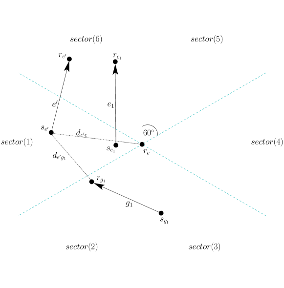
Figure 1: A depiction of the proof of Lemma 2.

We first consider the case that $e^{\prime}\in L^{\ell}$ is also a guard ($e^{\prime}=g_{j}$). In this case choose $g=e^{\prime}$, and $d_{e^{\prime}g}=d_{e^{\prime}}$. But $d_{e^{\prime}}\leq d_{e^{\prime}e}$ since $e^{\prime}\in L^{\ell}$, as required. We now consider the case that $e^{\prime}\in L^{\ell}\setminus G$. Given $e^{\prime}\in L^{\ell}\setminus G$, let $j$ denote the sector that contains $s_{e^{\prime}}$. We claim that $d_{e^{\prime}g_{j}}\leq 2\cdot d_{e^{\prime}e}$. Consider first $e^{\prime}=e_{j}$ (i.e., $s_{e_{j}}$ is a closest sender to $r_{e}$ in $\text{\emph{sector}}(j)$). Since $r_{g_{j}}$ is a closest receiver to $s_{e_{j}}$, we have $d_{e_{j}g_{j}}\leq d_{e_{j}}$. Since $e_{j}\in L^{\ell}$, we have $d_{e_{j}}\leq d_{e_{j}e}$. Thus, $d_{e_{j}g_{j}}\leq d_{e_{j}e}$, as required.

Consider now a link $e^{\prime}\neq e_{j}$. The following inequalities hold:

$$d_{e^{\prime}e} \geq d_{e_{j}e},\text{ ($s_{e_{j}}$ is a closest sender to $r_{e}$)}$$ (1)

$$d_{e^{\prime}g_{j}} \leq d_{s_{e^{\prime}}s_{e_{j}}}+d_{e_{j}g_{j}},\text{ (triangle ineq. in $\triangle s_{e^{\prime}}s_{e_{j}}r_{g_{j}}$)}$$ (2)

$$d_{e_{j}g_{j}} \leq d_{e_{j}e},\text{ (already proved for $e_{j}$)}$$ (3)

$$d_{s_{e^{\prime}}s_{e_{j}}} \leq d_{e^{\prime}e}.\text{ (proved below)}.$$ (4)

We now prove Eq. 4 (see Figure 2). Let $s^{*}$ denote the point along the segment from $r_{e}$ to $s_{e^{\prime}}$ such that $d_{s^{*}r_{e}}=d_{e_{j}e}$. The triangle $\triangle r_{e}s_{e_{j}}s^{*}$ is an isosceles triangle. Since $\angle s_{e_{j}}r_{e}s^{*}\leq 60^{\circ}$, it follows that the base angle $\angle r_{e}s_{e_{j}}s^{*}\geq 60^{\circ}$. Hence, $\angle r_{e}s_{e_{j}}s_{e^{\prime}}\geq\angle r_{e}s_{e_{j}}s^{*}\geq 60^{\circ}$. Since $\angle s_{e_{j}}r_{e}s_{e^{\prime}}\leq 60^{\circ}$, it follows that $d_{s_{e^{\prime}},s_{e_{j}}}\leq d_{e^{\prime}e}$, as required.

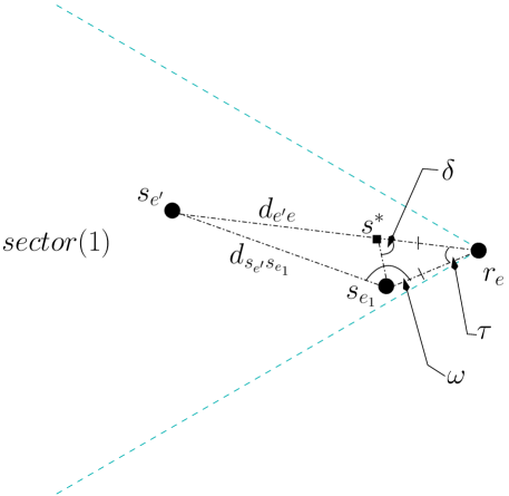
Figure 2: The triangle $\triangle r_{e}s_{e_{j}}s^{*}$ is an isosceles triangle. The angle $\tau\leq 60^{\circ}$. The angle $\delta\geq 60^{\circ}$. The angle $\omega\geq\delta\geq 60^{\circ}$.

To complete the proof that $d_{e^{\prime}g_{j}}\leq 2\cdot d_{e^{\prime}e}$, observe that

$$d_{e^{\prime}g_{j}}\stackrel{{\scriptstyle\text{eq.~{}\ref{eq:2}}}}{{\leq}}d_{s_{e^{\prime}}s_{e_{j}}}+d_{e_{j}g_{j}}\stackrel{{\scriptstyle\text{eqs.~{}\ref{eq:3},\ref{eq:4}}}}{{\leq}}d_{e^{\prime}e}+d_{e_{j}e}\stackrel{{\scriptstyle\text{eq.~{}\ref{eq:1}}}}{{\leq}}2\cdot d_{e^{\prime}e}.$$

∎

4.2 Necessary Conditions

Recall that Let $L\subseteq\mathcal{L}$ is an sinr-feasible set of links that belong to same bucket $B_{i}$. Let $e\in B_{i}$ denote an arbitrary link (not necessarily in $L$).

Lemma 3.

$$\sum_{e^{\prime}\in L^{\ell}}{\bar{a}}_{e^{\prime}}(e)=O(1).$$

Proof.

By Lemma 2, we find a set of “guards” $G\subseteq L^{\ell}$, such that:

1. $|G|\leq 6$,

2. $\forall e^{\prime}\in L^{\ell}~{}~{}\exists g\in G:d_{e^{\prime}g}\leq 2\cdot d_{e^{\prime}e}.$

First, let us bound $\sum_{e^{\prime}\in L^{\ell}\setminus G}{\hat{a}}_{e^{\prime}}(e)$,

$$\sum_{e^{\prime}\in L^{\ell}\setminus G}{\hat{a}}_{e^{\prime}}(e) <\sum_{e^{\prime}\in L^{\ell}\setminus G}2\cdot\left(\frac{d_{e^{\prime}}}{d_{e^{\prime}e}}\right)^{\alpha}$$

$$\leq 2^{\alpha+1}\cdot\sum_{e^{\prime}\in L^{\ell}\setminus G}\sum_{g\in G}\left(\frac{d_{e^{\prime}}}{d_{e^{\prime}g}}\right)^{\alpha}$$

$$\leq 2^{\alpha+2}\cdot\sum_{g\in G}\hat{a}_{L^{\ell}}(g)\>,$$ (5)

where the first line follows from Proposition 3. The second line follows from Lemma 2. The third line, again, follows from Proposition 3.

Since ${\bar{a}}_{e^{\prime}}(e)\leq 1$, we obtain

$$\sum_{e^{\prime}\in L^{\ell}}{\bar{a}}_{e^{\prime}}(e) \leq \sum_{e^{\prime}\in L^{\ell}\setminus G}{\bar{a}}_{e^{\prime}}(e)+|G|\>,$$ (6)

Hence,

$$\sum_{e^{\prime}\in L^{\ell}}{\bar{a}}_{e^{\prime}}(e) \leq \sum_{e^{\prime}\in L^{\ell}\setminus G}a_{e^{\prime}}(e)+|G|$$

$$= \sum_{e^{\prime}\in L^{\ell}\setminus G}\gamma_{e}\cdot{\hat{a}}_{e^{\prime}}(e)+|G|$$

$$\leq \gamma_{e}\cdot 2^{\alpha+2}\cdot\sum_{g\in G}\hat{a}_{L^{\ell}}(g)+|G|$$

$$\leq |G|\cdot\left(\frac{\gamma_{e}\cdot 2^{\alpha+2}}{\min_{g\in G}\gamma_{g}}+1\right)$$

$$\leq 6\left(\frac{(1+\varepsilon)\cdot 2^{\alpha+2}}{\varepsilon}+1\right)\>,$$

where the first line follows from Equation 6 and the fact that ${\bar{a}}_{e^{\prime}}(e)\leq a_{e^{\prime}}(e)$. The second line follows from the fact that $\gamma_{e}\cdot{\hat{a}}_{e^{\prime}}(e)=a_{e^{\prime}}(e)$. The third line follows from Equation 5. The fourth line follows since $L^{\ell}$ is sinr-feasible, that is, $a_{L^{\ell}}(g)\leq 1$ and $\hat{a}_{L^{\ell}}(g)\leq 1/\gamma_{g}$, for every $g\in G$. The last line follows from Proposition 2, Lemma 2, and $|G|\leq 6$. Since, $\alpha$ and $\varepsilon$ are constants, the lemma follows. ∎

Lemma 4.

$$\sum_{e^{\prime}\in L^{g}}{\bar{a}}_{e^{\prime}}(e)=O(1).$$

Proof.

Pick $e^{*}$ to be a shortest link in $L^{g}$. It follows from Proposition 3 and the triangle inequality (see Figure 3) that

$$\forall e^{\prime}\in L^{g}\setminus\{e^{*}\}:\hat{a}_{e^{\prime}}(e^{*})>\frac{1}{2}\cdot\left(\frac{d_{e^{\prime}}}{d_{e^{\prime}e^{*}}}\right)^{\alpha}\geq\frac{1}{2}\cdot\left(\frac{d_{e^{\prime}}}{d_{e^{\prime}e}+d_{e^{*}e}+d_{e^{*}}}\right)^{\alpha}\>.$$

Figure 3: The distance $d_{e^{\prime}e^{*}}$ is depicted by a bold segment. We bound $d_{e^{\prime}e^{*}}$ by applying the triangle inequality, that is the dashed segments and the length of link $e^{*}$, $d_{e^{*}}$.

Since $e^{\prime},e^{*}\in L^{g}$, it follows that $d_{e^{\prime}}>d_{e^{\prime}e}$ and $d_{e^{*}}>d_{e^{*}e}$. Since $d_{e^{\prime}}\geq d_{e}^{*}$ it follows that

$$\hat{a}_{e^{\prime}}(e^{*})>\frac{1}{2}\cdot\left(\frac{d_{e^{\prime}}}{3\cdot d_{e^{\prime}}}\right)^{\alpha}>\frac{1}{2}\cdot\frac{1}{3^{\alpha}}.$$

Since $a_{L^{g}}(e^{*})=\gamma_{e^{*}}\cdot{\hat{a}}_{L^{g}}(e^{*})$, it follows:

$$a_{L^{g}}(e^{*})=\gamma_{e^{*}}\cdot{\hat{a}}_{L^{g}}(e^{*})>\frac{1}{2}\cdot\frac{1}{3^{\alpha}}\cdot\gamma_{e^{*}}\cdot(|L^{g}|-1)\>.$$

Since $L^{g}$ is sinr-feasible, it follows that $a_{L^{g}}(e^{*})\leq 1$. Hence,

$$\frac{1}{2}\cdot\frac{1}{3^{\alpha}}\cdot\gamma_{e^{*}}\cdot(|L^{g}|-1) < 1\Rightarrow$$

$$|L^{g}| < 2\cdot 3^{\alpha}/\gamma_{e^{*}}+1\>.$$

Proposition 2 implies that $\frac{1}{\gamma_{e^{*}}}=O(1)$. Since $\alpha$ is a constant, it follows that $|L^{g}|=O(1)$. Since $\sum_{e^{\prime}\in L^{g}}{\bar{a}}_{e^{\prime}}(e)\leq|L^{g}|$, the lemma follows. ∎

Lemmas 3 and 4 imply the following theorem.

Theorem 1.

Let $L$ denote an SINR-feasible set of links. If $L\subseteq B_{i}$, then

$$\forall e\in B_{i}:~{}~{}~{}\sum_{\{e^{\prime}\in L:d_{e^{\prime}}\geq d_{e}\}}\bar{a}_{e^{\prime}}(e)~{}\leq~{}{\bar{a}}_{L}(e)+\bar{a}_{e}(e)=O(1).$$

The following theorem follows from  [Kes11, Thm 1]. The proof of the following theorem is in Appendix A.

Theorem 2.

Let $L$ denote an SINR-feasible set of links. If $L\subseteq B_{i}$, then

$$\forall e\in B_{i}:~{}~{}~{}\sum_{\{e^{\prime}\in L:d_{e^{\prime}}\geq d_{e}\}}\bar{a}_{e}(e^{\prime})=O(1).$$

5 LP Relaxation

In this section we formulate the linear program for the Max Throughput and Max-Min Throughput problems with arbitrary power assignments. The linear program formulation that we use for computing the multi-commodity flow $f$ is as follows.

$$\textsc{MaxTh}_{LP}:F^{*}=\text{maximize } |f|\text{ subject to}$$

$$f \in\mathcal{F}$$ (7)

$$\forall i~{}~{}\forall e \in B_{i}~{}~{}~{}f(e)+\sum_{\{e^{\prime}\in B_{i}:d_{e^{\prime}}\geq d_{e}\}}(\bar{a}_{e^{\prime}}(e)+\bar{a}_{e}(e^{\prime}))\cdot f(e^{\prime})\leq 1$$ (8)

$$\textsc{MaxMinTh}_{LP}:R^{*}= \text{maximize }\rho\text{ subject to}$$

$$f \in\mathcal{F}_{\rho}$$ (9)

$$\forall i~{}~{}\forall e \in B_{i}~{}~{}~{}~{}f(e)+\sum_{\{e^{\prime}\in B_{i}:d_{e^{\prime}}\geq d_{e}\}}(\bar{a}_{e^{\prime}}(e)+\bar{a}_{e}(e^{\prime}))\cdot f(e^{\prime})\leq 1$$ (10)

Recall that $\mathcal{F}$ denotes the polytope of all multi-commodity flows $f=(f_{1},\ldots,f_{k})$ such that $|f_{i}|\leq b_{i}$, for every $i$. Also recall that $\mathcal{F}_{\rho}\subseteq\mathcal{F}$ for $\rho>0$ denotes the polytope of all multi-commodity flows such that $|f_{i}|/b_{i}\geq\rho$. Constraints 7, 9 in $\textsc{MaxTh}_{LP}$ and $\textsc{MaxMinTh}_{LP}$ respectively require that the $f$ is a feasible multi-commodity flow with respect to $\mathcal{F}$ and $\mathcal{F}_{\rho}$.

Constraints  8, 10 in $\textsc{MaxTh}_{LP}$ and $\textsc{MaxMinTh}_{LP}$ respectively require that for every bucket $B_{i}$ and for every link $e\in B_{i}$ the amount of flow $f(e)$ plus the amount of the weighted symmetric interferences is bounded by one. Note that this symmetric interference constraint is with respect to links that are longer than $e$.

The objective function of $\textsc{MaxTh}_{LP}$ is to maximize the total flow $|f|$. The objective function of $\textsc{MaxMinTh}_{LP}$ is to maximize $\rho$, such that $f\in\mathcal{F}_{\rho}$. Namely, maximize $\min_{i=1\ldots k}|f_{i}|/b_{i}$.

We prove on Section 7 that the linear programs $\textsc{MaxTh}_{LP}$ and $\textsc{MaxMinTh}_{LP}$ are relaxations of the Max Throughput and Max-Min Throughput problems.

6 Algorithm

6.1 Algorithm description

For simplicity, we assume in this section that all the links are in the same bucket, that is $\mathcal{L}\subseteq B_{i}$ for some $i$. In Section 8 we show how to handle arbitrary power assignment. In Section 9 we extend the algorithm so that it assigns limited powers.

Algorithm overview.

We overview the algorithm for the Max Throughput problem. Assume for simplicity that, $\mathcal{L}\subseteq B_{i}$ for some $i$. First, the optimal flow $f^{*}$ is obtained by solving the linear program $\textsc{MaxTh}_{LP}$. We need to find an sinr-feasible schedule that supports a fraction of $f^{*}$. Second, we color the links using greedy multi-coloring. This coloring induces a preliminary schedule, in which every color class is “almost” sinr-feasible. This preliminary schedule is almost sinr-feasible since in every color class and every link $e$, the affectance of links that are longer than $e$ on $e$ is at most 1. However, the affectance of shorter links on $e$ may be still unbounded. Finally, we refine this schedule in order to obtain an sinr-feasible schedule. Note that the returned sinr-feasible schedule supports a fraction of the flow $f^{*}$. We show in Section 7 that this fraction is at least $\Omega(1/\log n)$.

Algorithm description.

The algorithm for the Max Throughput problem proceeds as follows.

1. Solve the linear program $\textsc{MaxTh}_{LP}$. Let $f^{*}$ denote the optimal solution.

2. Remove flow paths that traverse edges with $f^{*}(e)<1/(2nm)$. Let $\hat{f}$ denote the remaining flow.

3. Set $T=2nm$. Apply the greedy multi-coloring algorithm greedy-coloring (see Section 6.3) on the input $((\mathcal{L},\mathcal{L}^{2}),\hat{f},d,w,T)$, where the pair $(\mathcal{L},\mathcal{L}^{2})$ is a complete graph whose set of vertices is $\mathcal{L}$, for every link in $e\in\mathcal{L}$, $d(e)=d_{e}$, and $w(e,e^{\prime})\triangleq\bar{a}_{e}(e^{\prime})+\bar{a}_{e^{\prime}}(e)$ is a weight function over pair of links in $\mathcal{L}$. Let $\pi:\mathcal{L}\rightarrow 2^{\{0,\ldots T-1\}}$ denote the computed multi-coloring.

4. Apply procedure disperse to each color class $(\pi^{-1}(t))$, where $t\in\{0,\ldots T-1\}$. Let $\{L_{t,i}\}_{i=1}^{\ell(t)}$ denote the dispersed subsets.

5. Return the schedule $\{L_{t,i}\}_{t=0..T-1,i=1..\ell(t)}$ and the flow $f=(f_{1},\ldots,f_{k})$, where $f=\hat{f}/(2\cdot\ell(t))$.

Clearly steps 1 and 5 are polynomial. In Section 6.3 we show that step 3 is polynomial. In Section 6.4 we show that disperse is polynomial. Therefore, the running time of the algorithm is polynomial.

Remark 1.

The following changes are needed in order to obtain an algorithm for the Max-Min Throughput problem: (i) In Item 1 solve the linear program $\textsc{MaxMinTh}_{LP}$, (ii) in Item 2 remove flow paths that traverse edges with $f^{*}(e)<1/(2n^{2}km)$, (iii) in Item 3 set $T=2n^{2}km$.

6.2 Removing Minuscule Flow Paths

The greedy multi-coloring algorithm cannot support flows $f^{*}(e)<1/(2nm)$. We mitigate this problem simply by peeling off flow paths that traverse edges with a flow smaller than $1/(2nm)$. The formal description of this procedure is as follows. (1) Initialize $\hat{f}\leftarrow f$. (2) While there exists an edge $e$ with $\hat{f}(e)<1/(2nm)$, remove flow from $\hat{f}$ until $\hat{f}(e)=0$. This is done by computing flow paths for the flow that traverses $e$, and zeroing the flow along these paths.

6.3 Greedy Multi-Coloring

Let $G=(V,E)$ denote an undirected graph with edge weights $w:E\rightarrow[0,1]$ and node demands $x:V\rightarrow[0,1]$. Assume an ordering of the nodes induced by distinct node lengths $d(v)$. For a set $V^{\prime}\subset V$, let $w(V^{\prime},u)\triangleq\sum_{v\in V^{\prime}}w(v,u)$. Assume that

$$\forall u\in V:x(u)+\sum_{\{v\in V:d(v)>d(u)\}}w(v,u)\cdot x(v)\leq 1\>.$$ (11)

Indeed, Constraints 8, 10 in $\textsc{MaxTh}_{LP}$ and $\textsc{MaxMinTh}_{LP}$, respectively, imply that the input to the greedy coloring algorithm satisfies the assumption in Equation 11.

Lemma 5 (Greedy Coloring Lemma).

For every integer $T$, there is multi-coloring $\pi:V\rightarrow 2^{\{0,\ldots,T-1\}}$, such that

1. $\forall c\in\{0,\ldots,T-1\}~{}~{}\forall u\in\pi^{-1}(c):\sum_{\{v\in V:d(v)>d(u)\}}w(v,u)\leq 1$,

2. $\forall u\in V:|\pi(u)|\geq\lfloor x(u)\cdot T\rfloor$.

Algorithm 1 $\text{\emph{greedy-coloring}}((V,E),x,d,w,T)$ - greedy multi-coloring of $V$.

1. Scan the vertices in descending $d(v)$ length order, let $u$ denote the current node.

   1. $C^{\text{bad}}_{u}\leftarrow\{c\in\{0,\ldots,T-1\}:w(\pi^{-1}(c),u)>1\}$.

   2. If $|C^{\text{bad}}_{u}|>T-\lfloor x(u)\cdot T\rfloor$, then return “FAIL”.

   3. $\pi(u)\leftarrow$ first $\lfloor x(u)\cdot T\rfloor$ colors in $\{0,\ldots,T-1\}\setminus C^{\text{bad}}_{u}$.

2. Return $(\pi)$.

The running time of Algorithm 1 is at most $O(T^{2}\cdot|V|\cdot|E|)$. Since $T,|E|$ and $|V|$ are polynomial, it follows that the running time is polynomial.

Proof.

We apply a “first-fit” greedy multi-coloring listed in Algorithm 1. We now prove that this algorithm succeeds.

Let $b(u)\triangleq\lfloor x(u)\cdot T\rfloor$. Assume, for the sake of contradiction that, $|C^{\text{bad}}_{u}|>T-b(u)$, hence,

$$T-b(u)+1 \leq |C^{\text{bad}}_{u}|$$ (12)

$$\leq \sum_{c\in C^{\text{bad}}_{u}}w(\pi^{-1}(c),u)$$

$$\leq \sum_{\{v:d(u)<d(v)\}}|\pi(v)|\cdot w(v,u)$$

$$= \sum_{\{v:d(u)<d(v)\}}b(v)\cdot w(v,u)\>.$$

The third line follows from the fact that vertices are scanned in a descending length order, and by a rearrangement of the summation order. By adding $b(u)$ to both sides, we obtain:

$$T+1\leq\lfloor x(u)\cdot T\rfloor+\sum_{\{v:d(u)<d(v)\}}\lfloor x(v)\cdot T\rfloor\cdot w(v,u).$$ (13)

We divide Eq. 13 by $T$ to obtain a contradiction to Eq. 11, as required. We conclude, that the greedy coloring succeeds, and the lemma follows. ∎

6.4 The dispersion procedure disperse

The input to the dispersion procedure disperse consists of a set $L\subseteq\mathcal{L}$ of links that are assigned the same color by the multi-coloring procedure (see Algorithm 1 in Section 6.3). This implies that

$$\forall e\in L:\sum_{\{e^{\prime}\in L\setminus\{e\}:d_{e^{\prime}}\geq d_{e}\}}(\bar{a}_{e}(e^{\prime})+\bar{a}_{e^{\prime}}(e))\leq 1.$$ (14)

The dispersion procedure works in two phases. In the first phase, $L$ is partitioned into $\overline{1/3}$-signal sets $\{L_{i}\}_{i}$. In the second phase, each subset $L_{i}$ is further partitioned into $\overline{7/6}$-signal sets $\{L_{i}\}_{i=1}^{\ell(t)}$. Recall that a set of links $L_{i}$ is sinr-feasible if $L_{i}$ is a $\overline{(1+\varepsilon)}$-signal for some $\varepsilon>0$. Since every set in $\{L_{i}\}_{i=1}^{\ell(t)}$ is $\overline{(7/6)}$-signal, it follows that every set in $\{L_{i}\}_{i=1}^{\ell(t)}$ is sinr-feasible.

In Algorithm 2, we list the first phase of the dispersion procedure. Note that if a $\overline{1/3}$-signal set $J^{i}$ is always found in Line 2a, then $L$ is dispersed into at most $\log_{2}|L|$ subsets. In Lemma 8 we prove that this is indeed possible.

Algorithm 2 $\frac{1}{3}$-disperse$(L)$ : partition $L\subseteq\mathcal{L}$ into $O(\log n)$ $\overline{1/3}$-signal sets.

1. $i\leftarrow 0$ and $L^{0}\leftarrow L$.

2. while $L^{i}\neq\emptyset$ do

   1. find a $\overline{1/3}$-signal set $J^{i}\subseteq L^{i}$ such that $|J^{i}|\geq|L^{i}|/2$.

   2. $L^{i+1}\leftarrow L^{i}\setminus J^{i}$ and $i\leftarrow i+1$.

The second phase follows [HW09, Thm 1]. This phase is implemented by two first-fit bin packing procedures. In the first procedure, open $7$ bins, scan the links in some order and assign each link to the first bin in which its affectance is at most $3/7$. In the second procedure, partition each bin into $7$ sub-bins. Scan the links in the reverse order, and again, assign each link to the first bin in which its affectance is at most $3/7$.

Proposition 7 implies that step 2 in Algorithm 2 terminates after $O(\log m)$ iterations. Each of these iterations is polynomial. The second phase of the disperse algorithms is clearly polynomial. Therefore, the running time of the disperse algorithm is polynomial.

7 Algorithm Analysis

In this section we analyze the algorithm presented in Section 6. Recall that it is assumed that all the links are in the same bucket, that is $\mathcal{L}\subseteq B_{i}$ for some $i$. First, we prove that the linear program $\textsc{MaxTh}_{LP}$ is a fractional relaxation of the Max Throughput problem. We then show that the greedy coloring computes a schedule that supports the flow given by the LP. Unfortunately, this schedule is not an SINR-feasible schedule. We then prove that the refinement procedure (Step 4 of the algorithm) generates an SINR-feasible schedule with an $O(\log n)$ increase in the approximation ratio.

Let $f^{*}$ denote an optimal solution of the linear program $\textsc{MaxTh}_{LP}$, i.e., $F^{*}=|f^{*}|$. The following lemma shows that the linear program $\textsc{MaxTh}_{LP}$ is a relaxation of the Max Throughput problem.

Lemma 6.

There exists a constant $\lambda\geq 1$ such that, if $S=\{L_{t}\}_{t=0}^{T-1}$ is an sinr-feasible schedule that supports a multi-commodity flow $f$, then $f/\lambda$ is a feasible solution of the linear program $\textsc{MaxTh}_{LP}$. Hence, $F^{*}\geq|f|/\lambda$.

Proof.

Clearly $f/\lambda\in\mathcal{F}$. Thus, we only need to prove that $f/\lambda$ satisfies the constraint in Eq. 8. Consider an sinr-feasible set $L_{t}$ and an arbitrary link $e$. By, Theorems 1 and 2,

$$\sum_{\{e^{\prime}\in L_{t}:d_{e^{\prime}}\geq d_{e}\}}(\bar{a}_{e^{\prime}}(e)+\bar{a}_{e}(e^{\prime}))\leq O(1).$$

It follows that

$$\frac{1}{T}\cdot\sum_{t=0}^{T-1}\sum_{\{e^{\prime}\in L_{t}:d_{e^{\prime}}\geq d_{e}\}}(\bar{a}_{e^{\prime}}(e)+\bar{a}_{e}(e^{\prime}))\leq O(1).$$ (15)

Since $f(e^{\prime})\leq\frac{1}{T}\cdot|\{t:e^{\prime}\in L_{t}\}|$, We conclude that

$$\frac{1}{T}\cdot\sum_{t=0}^{T-1}\sum_{\{e^{\prime}\in L_{t}:d_{e^{\prime}}\geq d_{e}\}}(\bar{a}_{e^{\prime}}(e)+\bar{a}_{e}(e^{\prime})) \geq\sum_{\{e^{\prime}\in{\cal L}:d_{e^{\prime}}\geq d_{e}\}}(\bar{a}_{e^{\prime}}(e)+\bar{a}_{e}(e^{\prime}))\cdot f(e^{\prime}).$$ (16)

Since $f(e)\leq 1$, we conclude from Eqs. 15 and 16 that

$$f(e)+\sum_{\{e^{\prime}\in{\cal L}:d_{e^{\prime}}\geq d_{e}\}}(\bar{a}_{e^{\prime}}(e)+\bar{a}_{e}(e^{\prime}))\cdot f(e^{\prime})\leq O(1).$$ (17)

Let $\lambda>0$ denote a constant that bounds the left-hand side in Eq. 17. Then, $f/\lambda$ satisfies the constraints in Eq. 8, as required, and the lemma follows. ∎

Analogously, one could prove also that the linear program $\textsc{MaxMinTh}_{LP}$ is a relaxation of the Max-Min Throughput problem.

Lemma 7.

Suppose $S=\{L_{t}\}_{t=0}^{T-1}$ is an sinr-feasible schedule that supports a multi-commodity flow $f$. If $\rho\triangleq\min_{i=1\ldots k}|f_{i}|/b_{i}$, $R^{*}\geq\rho/\lambda$, for the same constant $\lambda\geq 1$ in Lemma 6.

The following proposition gives a lower bound on the optimal throughput.

Proposition 4.

$F^{*}\geq\frac{1}{n}$ and $R^{*}\geq\frac{1}{n^{2}k}$.

Proof.

Without loss of generality, the source and destination of each request are connected. Pick a request $R_{i}$ and a path $p_{i}$ from ${\hat{s}}_{i}$ to ${\hat{t}}_{i}$. Consider the schedule that schedules the links of $p_{i}$ in a round-robin fashion. Clearly, this schedule supports a flow $f=1/|p|$ from ${\hat{s}}_{i}$ to ${\hat{t}}_{i}$ along $p$, where $|p|$ denotes the length of $p$. This implies that $F^{*}\geq 1/n$, as required. The second part of the proposition is proved by concatenating $k$ schedules, one schedule per request. The concatenated schedule supports a flow $f=(f_{1},\ldots,f_{k})$, where $f_{i}=1/(nk)$ along the path $p_{i}$. Since $b_{i}\leq n$, it follows that $|f_{i}|/b_{i}\geq 1/(n^{2}k)$, and the proposition follows. ∎

Proposition 5.

$|{\hat{f}}|\geq\ F^{*}/2$

Proof.

Let us denote by $g$ the total flow that was removed in step 2. The contribution to the flow amount $|g|$ due to edges with small flow is less than $1/(2nm)$. Since there are $m$ edges, it follows that $|g|\leq 1/(2n)$. By Prop. 4 we have $F^{*}\geq\frac{1}{n}$, and the proposition follows. ∎

For the case of $\textsc{MaxMinTh}_{LP}$, one can show a similar result, that is $|{\hat{f}}|\geq\ R^{*}/2$.

Proposition 6.

If $~{}T\geq 2nm$, then the greedy multi-coloring algorithm computes a multi-coloring $\pi$ that induces a schedule that supports ${\hat{f}}/2$.

Proof.

Recall that a schedule $S=\{L_{t}\}_{t=0}^{T-1}$ induced by a multi-coloring $\pi:\mathcal{L}\rightarrow 2^{\{0,\ldots,T-1\}}$ is defined by $\forall t:~{}L_{t}=\pi^{-1}(t)$, where $\pi^{-1}(t)\triangleq\{e:t\in\pi(e)\}$. Also recall that a schedule $S$ supports $\hat{f}$ if $\forall e\in\mathcal{L}:~{}~{}~{}T\cdot{\hat{f}}(e)\leq\left|\{t\in\{0,\ldots,T-1\}:e\in L_{t}\}\right|$. Lemma 5 implies that the greedy multi-coloring algorithm (see the listing in Algorithm 1) computes multi-coloring $\pi$ such that $\forall e\in\mathcal{L}:|\pi(e)|\geq\lfloor{\hat{f}}(e)\cdot T\rfloor$. Hence, it suffices to prove that $T\cdot\hat{f}(e)/2\leq\lfloor T\cdot\hat{f(e)}\rfloor$, for every edge $e$. Indeed, step 2 in the algorithm (see listing in Sec. 6) implies that if $\hat{f}(e)>0$, then $\hat{f}(e)\geq 1/T$. Let us consider the following two cases: (1) If $\hat{f}(e)\in[1/T,2/T)$, then $T\cdot\hat{f(e)}/2<1=\lfloor T\cdot\hat{f(e)}\rfloor$, (2) if $\hat{f}(e)\geq 2/T$, then $T\cdot\hat{f(e)}/2\leq T\cdot(\hat{f}(e)-1/T)\leq\lfloor T\cdot\hat{f}(e)\rfloor$, as required. ∎

For the case of $\textsc{MaxMinTh}_{LP}$, one can show the same result if $T\geq 2n^{2}km$.

Lemma 8.

If $L\subseteq\mathcal{L}$ satisfies Eq. 14, then there exists a subset $J\subseteq L$ such that: (i) $J$is a $\overline{1/3}$-signal, and (ii) $|J|\geq|L|/2$.

Proof.

Define a square matrix $A$, the rows and columns of which are indexed by $L$ as follows: order $L$ in descending length order, so that $e^{\prime}$ precedes $e$ if $d_{e^{\prime}}>d_{e}$. Let $A({e,e^{\prime}})\triangleq(\bar{a}_{e}(e^{\prime})+\bar{a}_{e^{\prime}}(e))$ and $A(e,e)=0$. Note that $A$ is symmetric.

Let $A^{\Delta}$ denote the upper right triangular submatrix of $A$. Eq. 14 implies that,

$$\sum_{\{e^{\prime}:d_{e^{\prime}}\geq d_{e}\}}A(e^{\prime},e)\leq 1.$$

Hence, the weight of every column in $A^{\Delta}$ is bounded by $1$. This implies that the sum of the entries in $A^{\Delta}$ is bounded by $|L|$. By Markov’s Inequality, at most half the rows in $A^{\Delta}$ have weight greater than $2$. Let $J\subseteq L$ denote the indexes of the rows in $A^{\Delta}$ whose weight is at most $2$. Clearly, $|J|\geq|L|/2$.

We claim that, for every $e\in J$, the weight of the column $A^{e}$ is at most $3$. Indeed, $\sum_{\{e^{\prime}:d_{e^{\prime}}\geq d_{e}\}}A(e^{\prime},e)\leq 1$. In addition, $\sum_{\{e^{\prime}:d_{e^{\prime}}<d_{e}\}}A(e^{\prime},e)=\sum_{\{e^{\prime}:d_{e^{\prime}}<d_{e}\}}A(e,e^{\prime})\leq 2$ since this is the sum of the row indexed $e$ in $A^{\Delta}$. This implies that ${\bar{a}}_{J}(e)\leq 3$, for every $e\in J$, and the lemma follows. ∎

Proposition 7.

The dispersion procedure partitions every color class $\pi^{-1}(t)$ into $O(\log m)$ sinr-feasible sets.

Proof.

Recall that the dispersion procedure disperse consists of two phases. The first phase is the $\frac{1}{3}$-disperse$(\pi^{-1}(t))$ algorithm (see the listing in Algorithm 2), and the second phase is implemented by two first-fit packing procedures.

Let us consider the first phase. Note that $L^{0}=\pi^{-1}(t)$. Since $|L^{i+1}|\leq|L^{i}|/2$, then $\frac{1}{3}$-disperse$(\pi^{-1}(t))$ requires at most $\log_{2}|\pi^{-1}(t)|$ iterations. Hence, it partitions $\pi^{-1}(t)$ into at most $\log_{2}|\pi^{-1}(t)|$ sets, where each set is a $\overline{1/3}$-signal set.

Now, in the second phase each of these sets is partitioned into $49$ subsets. The lemma follows. ∎

Theorem 3.

If Assumption 1 holds, and all the links are in the same bucket, then there exists an $O(\log n)$-approximation algorithm for the Max Throughput and the Max-Min Throughput problems.

Proof.

Let opt denote the maximum total throughput. By Lemma 6, $F^{*}\geq\text{{opt}}/\lambda=\Omega(\text{{opt}})$. Recall that $f^{*}$ denotes an optimal solution of $\textsc{MaxTh}_{LP}$. By Prop. 5 $|\hat{f}|\geq|f^{*}|/2$, and by Prop. 6, the multi-coloring $\pi$ supports $\hat{f}/2$. By Prop. 7, the dispersion procedure reduces the throughput by a factor of $O(\log m)$. Since there are no parallel edges, $\log m=O(\log n)$. Thus, the final throughput is $|\hat{f}|/O(\log n)=\text{{opt}}/O(\log n)$, and the theorem follows. ∎

Since in the linear power assignment all links receive with same power, all the links are in the same bucket. We conclude with the following result for the linear power assignment.

Corollary 4.

If Assumption 1 holds, then there exists an $O(\log n)$-approximation algorithm for the Max Throughput and the Max-Min Throughput problems in the linear power assignment.

8 Given Arbitrary Transmission Powers

In this section we show how to apply the algorithm presented in Section 6 to the case in which transmission power $P_{e}$ of each link $e$ is part of the input. Note that $P_{e}$ may be arbitrary.

Theorem 5.

If Assumption 1 holds, then there exists an $O(\log n\cdot(\log\Delta+\log\Gamma))$-approximation algorithm for the Max Throughput and the Max-Min Throughput problems when the link transmission powers are part of the input.

Proof sketch: We construct an sinr-feasible schedule and its supported flow. The construction proceeds as follows: (1) solve the matching LP, (2) remove the minuscule flow paths as described in Item 2, (3) run Items 3-5 for every bucket separately, (4) concatenate the output schedules, to obtain an sinr-feasible schedule of all the links in $\mathcal{L}$. Step (3) of this construction reduces the flow by a factor of at most $O(\log n)$. Step (4) of this construction reduces the flow by an additional factor of at most the number of nonempty buckets, that is $O(\log\Delta+\log\Gamma)$. ∎

9 Limited Powers

In this section we consider the case in which the algorithm needs to assign a power $P_{e}$ to each link. The assigned powers must satisfy $P_{\min}\leq P_{e}\leq P_{\max}$. To simplify the description, assume that $\log_{2}(P_{\max}/P_{\min})$ is an integer, denoted by $\ell$.

We reduce this problem to the case of given arbitrary powers as follows. For each pair of nodes $(u,v)$, define $\ell+1$ parallel links, where the transmission power of the $i$th copy equals $2^{i}\cdot P_{\min}$.

Theorem 6.

Assume that, for every link $e$, $(P_{\min}/d_{e}^{\alpha})/N\geq(1+\varepsilon)\cdot\beta$. Then, there exists an $O((\log n+\log\log\Gamma)\cdot(\log\Delta+\log\Gamma))$-approximation algorithm for the Max Throughput and the Max-Min Throughput problems when the link transmission powers are in the range $[P_{\min},P_{\max}]$.

Proof sketch: Note that the number of links increases by a factor of $O(\log\Gamma)$. This implies that the $\log n$ factor increases to $(\log n+\log\log\Gamma)$.

The important observation is that there exists a solution that uses the discrete power assignments $2^{i}\cdot P_{e}$ and achieves a throughput that is a constant fraction of the optimal throughput. The theorem follows then from Theorem 5.

The proof of this observation proceeds as follows. Given an optimal schedule, refine each time slot so that it is a $p$-signal for $p=2$. This reduces the throughput only by a constant factor (see  [HW09, Thm 1]). Round up each transmission power to the smallest discrete power that satisfies Assumption 1. This increases the affectance by at most a factor of two, thus the resulting schedule is sinr-feasible. Moreover, the schedule uses links with powers that satisfy Assumption 1. ∎

Acknowledgments

We thank Nissim Halabi and Moni Shahar for useful conversations. This project was partially funded by the Israeli ministry of Science and Technology.

Appendix A Proofs

Proposition 3.

$$\forall i~{}\forall~{}e_{1},e_{2}\in B_{i}:~{}~{}\frac{1}{2}\cdot\left(\frac{d_{e_{1}}}{d_{e_{1}e_{2}}}\right)^{\alpha}<\hat{a}_{e_{1}}(e_{2})<2\cdot\left(\frac{d_{e_{1}}}{d_{e_{1}e_{2}}}\right)^{\alpha}\>,$$

$$\forall~{}e_{1},e_{2}\in\mathcal{L}:~{}~{}\hat{a}_{e_{1}}(e_{2})=\left(\frac{d_{e_{2}}}{d_{e_{1}e_{2}}}\right)^{\alpha}\text{ in the uniform power model.}$$

Proof.

Recall that $\hat{a}_{e^{\prime}}(e)\triangleq\frac{S_{e^{\prime}e}}{S_{e}}$, $S_{e}\triangleq P_{e}/d_{e}^{\alpha}$, and $S_{e^{\prime}e}=P_{e^{\prime}}/{d_{e^{\prime}e}^{\alpha}}$. Note that every two links $e_{1},e_{2}\in B_{i}$, satisfy that $S_{e_{1}}/S_{e_{2}}\in(1/2,2)$. Hence,

$$\hat{a}_{e_{1}}(e_{2}) = \frac{S_{e_{1}e_{2}}}{S_{e_{2}}}=\frac{S_{e_{1}e_{2}}}{S_{e_{1}}}\cdot\frac{S_{e_{1}}}{S_{e_{2}}}$$

$$= \frac{P_{e_{1}}/d_{e_{1}e_{2}}^{\alpha}}{P_{e_{1}}/d_{e_{1}}^{\alpha}}\cdot\frac{S_{e_{1}}}{S_{e_{2}}}$$

$$= \left(\frac{d_{e_{1}}}{{d_{e_{1}e_{2}}}}\right)^{\alpha}\cdot\frac{S_{e_{1}}}{S_{e_{2}}}\>,$$

as required.

On the other hand, in the uniform power model assignment, all links transmit with the same power, namely $P_{e}=P_{e^{\prime}}$ for every two links $e$ and $e^{\prime}$. Hence,

$$\hat{a}_{e_{1}}(e_{2}) = \frac{S_{e_{1}e_{2}}}{S_{e_{2}}}$$

$$= \frac{P_{e_{1}}/d_{e_{1}e_{2}}^{\alpha}}{P_{e_{2}}/d_{e_{2}}^{\alpha}}$$

$$= \left(\frac{d_{e_{2}}}{{d_{e_{1}e_{2}}}}\right)^{\alpha}\>,$$

as required. ∎

Theorem 2

Let $L$ denote an SINR-feasible set of links. If $L\subseteq B_{i}$, then

$$\forall e\in B_{i}:~{}~{}~{}\sum_{\{e^{\prime}\in L:d_{e^{\prime}}\geq d_{e}\}}\bar{a}_{e}(e^{\prime})=O(1).$$

Proof.

Theorem 1 in  [Kes11] implies that

$$\sum_{\{e^{\prime}\in L:d_{e^{\prime}}\geq d_{e}\}}\min\left\{1,\left(\frac{d_{e}}{d_{ee^{\prime}}}\right)^{\alpha}\right\}+\sum_{\{e^{\prime}\in L:d_{e^{\prime}}\geq d_{e}\}}\min\left\{1,\left(\frac{d_{e}}{d_{s_{e^{\prime}}r_{e}}}\right)^{\alpha}\right\}=O(1).$$

It follows that,

$$O(1) = \sum_{\{e^{\prime}\in L:d_{e^{\prime}}\geq d_{e}\}}\min\left\{1,\left(\frac{d_{e}}{d_{ee^{\prime}}}\right)^{\alpha}\right\}$$

$$\geq \sum_{\{e^{\prime}\in L:d_{e^{\prime}}\geq d_{e}\}}\min\left\{1,\frac{1}{2}\cdot{\hat{a}}_{e}(e^{\prime})\right\}$$

$$= \sum_{\{e^{\prime}\in L:d_{e^{\prime}}\geq d_{e}\}}\min\left\{1,\frac{1}{2\cdot\gamma_{e^{\prime}}}\cdot a_{e}(e^{\prime})\right\}$$

$$\geq \sum_{\{e^{\prime}\in L:d_{e^{\prime}}\geq d_{e}\}}\min\left\{1,\frac{\varepsilon}{2\cdot(1+\varepsilon)\cdot\beta}\cdot a_{e}(e^{\prime})\right\}\>,$$

where the second line follows since $L\subseteq B_{i}$ and Proposition 3. The third line follows from the definition of $a_{e}(e^{\prime})$. The last line follows from Proposition 2. The theorem follows, since $\frac{\varepsilon}{2\cdot(1+\varepsilon)\cdot\beta}=O(1)$ and since $\bar{a}_{e^{\prime}}(e)\triangleq\min\{1,a_{e^{\prime}}(e)\}$. ∎

References

- [ABL05] M. Alicherry, R. Bhatia, and L.E. Li. Joint channel assignment and routing for throughput optimization in multi-radio wireless mesh networks. In MobiCom, pages 58–72. ACM, 2005.
- [Cha09] D.R. Chafekar. Capacity Characterization of Multi-Hop Wireless Networks-A Cross Layer Approach. PhD thesis, Virginia Polytechnic Institute and State University, 2009.
- [CKM+07] D. Chafekar, VS Kumar, M.V. Marathe, S. Parthasarathy, and A. Srinivasan. Cross-layer latency minimization in wireless networks with SINR constraints. In MobiHoc, pages 110–119. ACM, 2007.
- [CKM+08] D. Chafekar, VSA Kumart, M.V. Marathe, S. Parthasarathy, and A. Srinivasan. Approximation algorithms for computing capacity of wireless networks with SINR constraints. In INFOCOM 2008, pages 1166–1174, 2008.
- [FKV10] A. Fanghänel, T. Kesselheim, and B. Vöcking. Improved algorithms for latency minimization in wireless networks. Theoretical Computer Science, 2010.
- [Gal68] R.G. Gallager. Information theory and reliable communication. John Wiley & Sons, Inc. New York, NY, USA, 1968.
- [GK00] P. Gupta and P.R. Kumar. The capacity of wireless networks. IEEE Transactions on information theory, 46(2):388–404, 2000.
- [GOW07] O. Goussevskaia, Y.A. Oswald, and R. Wattenhofer. Complexity in geometric SINR . In MobiHoc, pages 100–109. ACM, 2007.
- [GWHW09] O. Goussevskaia, R. Wattenhofer, M. Halldórsson, and E. Welzl. Capacity of arbitrary wireless networks. In INFOCOM 2009, pages 1872–1880, 2009.
- [Hal09] M. Halldórsson. Wireless scheduling with power control. ESA 2009, pages 361–372, 2009.
- [HM11a] M. Halldórsson and P. Mitra. Wireless Capacity with Oblivious Power in General Metrics. In SODA, 2011.
- [HM11b] M.M. Halldorsson and P. Mitra. Nearly optimal bounds for distributed wireless scheduling in the sinr model. Arxiv preprint arXiv:1104.5200, 2011.
- [HW09] M. Halldórsson and R. Wattenhofer. Wireless Communication is in APX. Automata, Languages and Programming, pages 525–536, 2009.
- [Kes11] T. Kesselheim. A constant-factor approximation for wireless capacity maximization with power control in the SINR model. In Proceedings of the 22nd ACM-SIAM Symposium on Discrete Algorithms (SODA), 2011.
- [KV10] T. Kesselheim and B. Vöcking. Distributed contention resolution in wireless networks. Distributed Computing, pages 163–178, 2010.
- [LSS06] X. Lin, N.B. Shroff, and R. Srikant. A tutorial on cross-layer optimization in wireless networks. Selected Areas in Communications, IEEE Journal on, 24(8):1452–1463, 2006.
- [MW06] T. Moscibroda and R. Wattenhofer. The complexity of connectivity in wireless networks. In Proc. of the 25th IEEE INFOCOM. Citeseer, 2006.
- [Ton10] T. Tonoyan. Algorithms for Scheduling with Power Control in Wireless Networks. Arxiv preprint arXiv:1010.5493, 2010.
- [Wan09] P.J. Wan. Multiflows in multihop wireless networks. In MobiHoc, pages 85–94. ACM, 2009.
- [WFJ+11] P.J. Wan, O. Frieder, X. Jia, F. Yao, X. Xu, and S. Tang. Wireless link scheduling under physical interference model. 2011.