Negative Example Aided Transcription Factor Binding Site Search

Abstract

Computational approaches to transcription factor binding site identification have been actively researched for the past decade. Negative examples have long been utilized in de novo motif discovery and have been shown useful in transcription factor binding site search as well. However, understanding of the roles of negative examples in binding site search is still very limited.

We propose the 2-centroid and optimal discriminating vector methods, taking into account negative examples. Cross-validation results on E. coli transcription factors show that the proposed methods benefit from negative examples, outperforming the centroid and position-specific scoring matrix methods. We further show that our proposed methods perform better than a state-of-the-art method. We characterize the proposed methods in the context of the other compared methods and show that, coupled with motif subtype identification, the proposed methods can be effectively applied to a wide range of transcription factors. Finally, we argue that the proposed methods are well-suited for eukaryotic transcription factors as well.

Software tools are available at: http://biogrid.engr.uconn.edu/tfbs_search/.

1 Introduction

Transcription of genes followed by translation of their transcripts into proteins determines the type and functions of a cell. Expression of certain genes even initiates or suppresses differentiation of stem cells. It is therefore crucial to understand the mechanisms of transcriptional regulation. Among them, transcription factor (TF) binding is the one that has been given considerable attention by computational biologists for the past decade and is still being actively researched. A TF is a protein or protein complex that regulates transcription of one or more genes by binding to the double-stranded DNA. A first step in computational identification of target genes regulated by a TF is to pinpoint its binding sites in the genome. Once the binding sites are found, the putative target genes can be searched and located in flanking regions of the binding sites.

In general, there are two approaches to computational transcription factor binding site (TFBS) identification, motif discovery and TFBS search. The former assumes that a set of sequences is given and each of the sequences may or may not contain TFBS’s. An algorithm then predicts the locations and lengths of TFBS’s. The term motif refers to the pattern that are shared by the discovered TFBS’s. This kind of algorithms relies on no prior knowledge of the motif and hence is known as de novo motif discovery algorithms. The latter assumes that, in addition to a set of sequences, the locations and lengths of TFBS’s are known. An algorithm then learns from these examples and predicts TFBS’s in new sequences. Such algorithms are also called supervised learning algorithms since they are guided by the given sequences with known TFBS’s.

Plenty of efforts have been devoted to the de novo motif discovery problem [1, 2, 3, 4, 5, 6, 7, 8, 9, 10, 11]. Comprehensive evaluation and comparison of the developed tools have been performed by Tompa et al. [12] and Hu et al. [13]. In this study, we focus on the problem of TFBS search. We refer readers interested in the motif discovery problem to the evaluation and review articles [12, 13, 14] and references therein.

A typical TFBS search method searches for the binding sites of a particular transcription factor in the following manner. It scans a target DNA sequence and compare each $l$-mer to the binding site profile of the TF, where $l$ is the length of a binding site. Each of the $l$-mer is scored when comparing to the profile. A cut-off score is then set by the method to select candidate TF binding sites. The position-specific scoring matrix is a widely used profile representation, where the binding sites of a TF are encoded as a $4\times l$ matrix. Column $i$ of the matrix stores the scores of matching the $i^{\text{th}}$ letter in an $l$-mer to nucleotides A, C, G and T, respectively. Depending on the method of choice, the score of A at position $i$ can be the count of A at position $i$ in the known TFBS’s, the log-transformed probability of observing A at position $i$, or any other reasonable number.

Plenty of novel methods were based on this simple scoring method. Osada et al. [15] extended this scoring approach by considering pairs of nucleotides and weighting nuclueotide and nucleotide pairs by information content. Extensive leave-one-out (LOO) cross-validation (CV) experiments were conducted on 35 TF’s with totally 410 binding sites. The results showed significant improvement regardless of the model used for motif representation. In a recent study, Salama and Stekel[20] showed correlations between two nucleotides within a TFBS by plotting the mutual information matrix of a motif, reinforcing the findings reported in [15]. A novel scoring method called the ungapped likelihood under positional background (ULPB) method was proposed in this study. The ULPB method models a TFBS by two first-order Markov chains and scores a candidate binding site by likelihood ratio produced by the two Markov chains. LOO results on 22 TF’s with 20 or more binding sites showed that ULPB is superior to the methods compared in their work.

Explicit use of negative examples in the TFBS search problem is hindered by the vast amount of non-binding sites of a transcription factor. This is further aggravated by the low specificity of some transcription factors, where a binding site may be more similar to a non-binding site than some other binding sites. Due to these issues, previous studies involving negative examples are limited and the roles of negative examples remain unclear. In a review article, Hannenhalli [17] surveyed work on improved motif models and integrative methods. None of these reviewed studies [17], however, investigated the use of negative examples on top of true TFBS’s. While introducing improved benchmarks for computational motif discovery, Sandve et al. [16] described algorithms for finding optimal motif models using both positive and negative TFBS’s. Three models were compared using the proposed benchmarks. However, no methods relying on only positive examples were compared. Recently, Do and Wang [18] formulated the TFBS search problem as a classification problem, proposed a novel similarity measure, and investigated three classification techniques. Five-fold CV results showed that learning vector quantization performed better than P-Match [19], which requires only positive examples. The evaluation, however, was done on only 8 human transcription factors and 8 artificial ones. It is not clear how the results on the small set of 8 real TF’s can be related to other TF’s.

The goal of this study is to investigate the inclusion of negative examples in addition to positive ones in TFBS search. We propose and characterize two novel extensions of the centroid method introduced in [15]. Besides the sequence similarity measures employed in [15], we also incorporate the novel similarity measure in [18] into an extension of the centroid method. We compare our proposed methods to methods that do not rely upon negative examples, that is, the centroid method, the ULPB method [20] and the well-known position-specific scoring matrix method. Performance of a method is assessed by LOO CV experiments on two data sets of 35 and 26 transcription factors, respectively. Moreoever, we discuss the situations when the proposed methods can accurately differentiate binding sites from non-binding sites. Advantages of coupling motif subtype identification with the proposed methods are also discussed.

The paper is organized as follows. In Section 2, we introduce existing methods compared in this study and describe two novel methods proposed in this work. Leave-one-out cross-validation results on two data sets are presented in Section 3. In Section 4, properties of the proposed methods are studied and discussed. Connections between the proposed methods and the other compared methods are established. Finally, we give the concluding remarks in Section 5.

2 Methods

2.1 Data sets

For ease of comparison, we conduct experiments on two data sets used in previous work.The first set was collected by Osada et al. [15], which consists of 410 binding sites of 35 TF’s with flanking regions located in the E. coli K-12 genome (version M54 of strain MG1655[21]). The statistics of this data set are listed in Table I. The second one also contains binding sites of TF’s in the E. coli K-12 genome and was considered in [20]. We downloaded the latest data (release 6.8) from RegulonDB [22] and kept only 26 TF’s with 17 or more known binding sites. We summarize the data set in Table II.

TABLE I: Statistics of the first data set with 35 TF’s

Name	Length	# TFBS’s	Name	Length	# TFBS’s
araC	48	6	arcA	15	13
argR	18	17	cpxR	15	12
crp	22	49	cspA	20	4
cytR	18	5	dnaA	15	8
fadR	17	7	fis	35	19
fnr	22	13	fruR	16	12
fur	18	9	galR	16	7
gcvA	20	4	glpR	20	13
hipB	30	4	ihf	48	26
lexA	20	19	lrp	25	14
malT	10	10	metJ	16	15
metR	15	8	nagC	23	6
narL	16	10	ntrC	17	5
ompR	20	9	oxyR	39	4
phoB	22	15	purR	26	22
soxS	35	14	torR	10	4
trpR	24	4	tus	23	6
tyrR	22	17

TABLE II: Statistics of the second data set with 26 TF’s

Name	Length	# TFBS’s	Name	Length	# TFBS’s
MetJ	8	29	Lrp	12	62
SoxS	18	19	H-NS	15	37
FlhDC	16	20	AraC	18	20
Fis	15	206	ArcA	15	93
IHF	13	101	OmpR	20	22
PhoB	20	17	GlpR	20	23
OxyR	17	41	CpxR	15	37
NarL	7	90	CRP	22	249
TyrR	18	19	NarP	7	20
Fur	19	81	LexA	20	40
NtrC	17	17	FNR	14	87
MalT	10	20	PhoP	17	21
ArgR	18	32	NsrR	11	37

2.2 The centroid and 2-centroid methods

We introduce the centroid method proposed by Osada et al. [15] in a different manner. We first define the similarity measure between two sequences $s$ and $t$ of length $l$.

$$\mathrm{Sim}(s,t)=\sum_{i=1}^{l}w_{i}\mathcal{I}_{s_{i}}(t_{i}),$$ (1)

where $s_{i}$ ($t_{i}$) is the $i^{\text{th}}$ letter of $s$ ($t$), $w_{i}$ denotes the weight on the $i^{\text{th}}$ letter and $\mathcal{I}_{s_{i}}(\cdot)$ is the indicator function given by

$$\mathcal{I}_{s_{i}}(t_{i})=\left\{\begin{array}[]{cc}1&\text{if }t_{i}=s_{i},\\ 0&\text{otherwise.}\end{array}\right.$$

In this work, $w_{i}$ is set to either $1$ or the information content at position $i$ defined as

$$IC_{i}=2+\sum_{u\in\{\text{A, C, G, T}\}}f_{i}(u)\log_{2}\left[f_{i}(u)\right],$$ (2)

where $f_{i}(u)$ is the probability of observing letter $u$ at position $i$. When $w_{i}=1$ for all $i$, $\mathrm{Sim}(s,t)$ simply counts the number of letters shared between $s$ and $t$. When pairs of nucleotides are taken into account, the similarity measure is defined as follows:

$$\mathrm{Sim2}(s,t)=\mathrm{Sim}(s,t)+\sum_{k=1}^{K}\sum_{i=1}^{l-k}w_{i,j}\mathcal{I}_{s_{i}s_{j}}(t_{i}t_{j}),$$ (3)

where $j=i+k$ and $\mathcal{I}_{s_{i}s_{j}}(\cdot)$ is the indicator function given by

$$\mathcal{I}_{s_{i}s_{j}}(t_{i}t_{j})=\left\{\begin{array}[]{cc}1&\text{if }t_{i}=s_{i}\text{ and }t_{j}=s_{j},\\ 0&\text{otherwise.}\end{array}\right.$$

Similarly, $w_{i,j}$ is set to either $1$ or the information content of the nucleotide pair at $(i,j)$ given by

$$IC_{i,j}=4+\sum_{u,v\in\{\text{A, C, G, T}\}}f_{i,j}(u,v)\log_{2}\left[f_{i,j}(u,v)\right],$$ (4)

where $f_{i,j}(u,v)$ is the probability of observing letters $u$ and $v$ at positions $i$ and $j$, respectively. We consider only pairs that are at most 2 nucleotides apart ($K=2$) according to the results reported in [15].

To facilitate similarity computation, an l-mer $s$ can be easily embedded in $\mathbb{R}^{4l}$ while preserving the similarity measure in (1) by the dot product between two vectors. That is, letter $s_{i}$ is converted to 4 dummy variables – $\sqrt{w_{i}}\mathcal{I}_{\text{A}}(s_{i}),\sqrt{w_{i}}\mathcal{I}_{\text{C}}(s_{i}),\sqrt{w_{i}}\mathcal{I}_{\text{G}}(s_{i})\text{ and }\sqrt{w_{i}}\mathcal{I}_{\text{T}}(s_{i})$ for $i=1,2,\ldots,l$. Fig. 1 illustrates the transformation of an $l$-mer into a $4l$-element vector when $w_{i}=1$ for $i=1,2,\ldots,l$. Similarly, an l-mer can be transformed into a $(36l-48)$-element vector such that the similarity measure in (3) with $K=2$ is preserved, where a pair of nucleotides is converted to 16 dummy variables. Consequently, the similarity between two sequences $s$ and $t$, can be computed by $\bm{s}^{\mathrm{T}}\bm{t}$, where $\bm{s}$ and $\bm{t}$ denote sequences $s$ and $t$, respectively, embedded in the Euclidean space. In the rest of the paper, we denote a sequence $s$ embedded in the Euclidean space by the same symbol in bold, i.e., $\bm{s}$.

Figure 1: Illustration of embedding an $l$-mer in $\mathbb{R}^{4l}$ with $w_{i}=1$ for $i=1,2,\ldots,l$.

Consider a set $S$ of $n_{+}$ binding sites of length $l$ for a TF. The centroid method scores an l-mer $t$ by

$$\mathrm{Score}(t)=\frac{1}{n_{+}}\sum_{s\in S}\bm{s}^{\mathrm{T}}\bm{t}=\left(\frac{1}{n_{+}}\sum_{s\in S}\bm{s}\right)^{\mathrm{T}}\bm{t}=\bm{\mu}_{+}^{\mathrm{T}}\bm{t},$$ (5)

where $\bm{\mu}_{+}=\frac{1}{n_{+}}\sum_{s\in S}\bm{s}$ is the centroid of the binding sites in $S$.

Now, with a set $N$ of $n_{-}$ non-binding sites of length $l$ for the TF, a natural extension of the centroid method scores an l-mer $t$ by

$$\mathrm{Score}(t) =\bm{\mu}_{+}^{\mathrm{T}}\bm{t}-\frac{1}{n_{-}}\sum_{s\in N}\bm{s}^{\mathrm{T}}\bm{t}=\bm{\mu}_{+}^{\mathrm{T}}\bm{t}-\left(\frac{1}{n_{-}}\sum_{s\in N}\bm{s}\right)^{\mathrm{T}}\bm{t}$$

$$=(\bm{\mu}_{+}-\bm{\mu}_{-})^{\mathrm{T}}\bm{t},$$ (6)

where $\bm{\mu}_{-}=\frac{1}{n_{-}}\sum_{s\in N}\bm{s}$ is the centroid of the non-binding sites in $N$. We refer to this method as the 2-centroid method in the rest of the paper since it employs the centroids of the binding sites and the non-binding sites. Fig. 2 illustrates the centroid and 2-centroid methods when non-TFBS’s as well as TFBS’s are available. Alternatively, $\mathrm{Score}(t)$ in (6) can be interpreted as follows: It measures the average similarity of $t$ to all the binding sites, measures the average similarity of $t$ to all the non-binding sites and calculates the difference.

We note that $\mathrm{Score}(t)$ in (5) is proportional to $\mathrm{Score}(t)/||\bm{\mu}_{+}||$ , where $||\bm{\mu}_{+}||$ is the length of $\bm{\mu}_{+}$. Moreover, by virtue of the equality

$$\bm{\mu}_{+}^{\mathrm{T}}\bm{t}=||\bm{\mu}_{+}||\,\,||\bm{t}||\cos\theta,$$

we know $\mathrm{Score}(t)/||\bm{\mu}_{+}||$ equals the orthogonal projection of $\bm{t}$ onto $\bm{\mu}_{+}$, where $\theta$ is the angle formed by vectors $\bm{\mu}_{+}$ and $\bm{t}$ (see Fig. 3 for an illustration). The computation of $\mathrm{Score}(t)$ is therefore equivalent to computation of the orthogonal projection of $\bm{t}$ onto $\bm{\mu}_{+}$. Similarly, the computation of $\mathrm{Score}(t)$ in (6) is equivalent to computation of the orthogonal projection of $\bm{t}$ onto $\bm{\mu}_{+}-\bm{\mu}_{-}$.

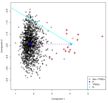
Figure 2: Illustration of the 2-centroid method. The solid arrow denotes vector $\bm{\mu}_{+}$, while the dashed arrow represents vector $\bm{\mu}_{+}-\bm{\mu}_{-}$, pointing from $\bm{\mu}_{-}$ to $\bm{\mu}_{+}$.

Figure 3: The orthogonal projection of $\bm{t}$ onto $\bm{\mu}_{+}$ is equal to $\mathrm{Score}(t)/||\bm{\mu}_{+}||\propto\mathrm{Score}(t)$.

2.3 Optimal scoring function

It can be seen that the scoring functions in (5) and (6) take the following form:

$$\mathrm{Score}(t)=\bm{\beta}^{\mathrm{T}}\bm{t},$$ (7)

where $\bm{\beta}=\bm{\mu}_{+}$ for the centroid method and $\bm{\beta}=\bm{\mu}_{+}-\bm{\mu}_{-}$ for the 2-centroid method. Therefore, an “optimal” $\bm{\beta}$ gives rise to an optimal scoring function with the most discriminating power.

We describe a way of finding an optimal $\bm{\beta}$. Suppose that $|S|=n_{+}$ and $|N|=n_{-}$, that is, there are $n_{+}$ binding sites and $n_{-}$ non-binding sites for a particular TF. Let $S=\{t_{(1)},t_{(2)},\ldots,t_{(n_{+})}\}$ and $N=\{t_{(n_{+}+1)},t_{(n_{+}+2)},\ldots,t_{(n)}\}$ , where $t_{(i)}$ denotes the $i^{\text{th}}$ l-mer in $S\cup N$ and $n=n_{+}+n_{-}$. We find the optimal $\bm{\beta}$ by solving the following minimization problem:

$$\min_{\bm{\beta},b,\bm{\xi}}\,\, \frac{1}{2}||\bm{\beta}||^{2}+\frac{C}{n_{+}}\sum_{i=1}^{n_{+}}\xi_{i}+\frac{C}{n_{-}}\sum_{i=n_{+}+1}^{n}\xi_{i}$$ (8)

subject to $$\frac{\mathrm{Score}(t_{(i)})}{||\bm{\beta}||}\geq\frac{b+1-\xi_{i}}{||\bm{\beta}||}\text{ for }t_{(i)}\in S,$$ (9)

$$\frac{\mathrm{Score}(t_{(i)})}{||\bm{\beta}||}\leq\frac{b-1+\xi_{i}}{||\bm{\beta}||}\text{ for }t_{(i)}\in N,$$ (10)

$$\xi_{i}\geq 0\,\,\forall i.$$ (11)

The constraint in (9) ensures that the projection of a TFBS $t_{(i)}$ onto the vector $\bm{\beta}$, $\frac{\mathrm{Score}(t_{(i)})}{||\bm{\beta}||}$, exceeds the threshold $\frac{b+1}{||\bm{\beta}||}$. On the other hand, the constraint in (10) ensures that the projection of a non-TFBS $t_{(i)}$ onto $\bm{\beta}$ stays below the threshold $\frac{b-1}{||\bm{\beta}||}$. Flexibility is given to the thresholds by introducing $\xi_{i}$’s with cost captured by the last two terms in (8), where $C$ is a positive parameter. Finally, to clearly distinguish TFBS’s from non-TFBS’s, the squared difference between the two thresholds ($\frac{b+1}{||\bm{\beta}||}$ and $\frac{b-1}{||\bm{\beta}||}$) is made as large as possible. This amounts to maximizing $\left(\frac{2}{||\bm{\beta}||}\right)^{2}$ or, equivalently, minimizing $\frac{1}{2}||\bm{\beta}||^{2}$, which is the first term in (8). We call this approach the optimal discriminating vector (ODV) method.

2.4 PSSM and ULPB

We briefly describe the PSSM (position-specific scoring matrix) methods used in [15, 20] and the ungapped likelihood under positional background method proposed by Salama and Stekel [20]. Consider a specific TF with binding sites of length $l$. The PSSM method used in [20] scores an $l$-mer $t$ by

$$\sum_{i=1}^{l}\log\left[f_{i}(t_{i})\right],$$ (12)

where no pair of nucleotides was considered for this model in [20]. We refer to this method as the position-specific probability matrix (PSPM) method to distinguish it from the PSSM used in [15].

The PSSM method given in [15] takes into account background probabilities and scores an $l$-mer by

$$\sum_{i=1}^{l}\log\left(\frac{f_{i}(t_{i})}{f(t_{i})}\right)w_{i},$$ (13)

where $f(u)$ is the probability of observing nucleotide $u\in\{$A, C, G, T$\}$. When nucleotide pairs are considered, the score becomes

$$\sum_{i=1}^{l}w_{i}\log\left(\frac{f_{i}(t_{i})}{f(t_{i})}\right)+\sum_{k=1}^{K}\sum_{i=1}^{l-k}w_{i,j}\log\left(\frac{f_{i,j}(t_{i},t_{j})}{f_{k}(t_{i},t_{j})}\right),$$ (14)

where $j=i+k$, $K=2$ and $f_{k}(u,v)$ is the background probability of observing letters $u$ and $v$ separated by $k-1$ arbitrary letters in between. For this method, we estimate the background probabilities using only the TFBS sequences as in [15].

The ULPB models a TFBS by a first-order Markov chain and models the background by another first-order Markov chain. The former depends on position-specific transition probability $f_{i}(v|u)$, which gives the probability of observing $v$ at the $(i+1)^{\text{th}}$ position given $u$ has been seen at position $i$, where $u,v\in\{\text{A, C, G, T}\}$ and $i=1,2,\ldots,l-1$. The latter depends on background transition probability $f(v|u)$, the probability of observing $v$ given $u$ has been observed at the previous position, where $u,v\in\{\text{A, C, G, T}\}$. For this method, the background transition probabilities are estimated using the entire genome of a species. The ULPB method scores an $l$-mer by

$$\log f_{1}(t_{1})+\sum_{i=1}^{l-1}\log\left(\frac{f_{i}(t_{i+1}|t_{i})}{f(t_{i+1}|t_{i})}\right).$$ (15)

Although Salama and Stekel [20] did not consider background probability in the first term of (15), the score is approximately the log-likelihood ratio of the two Markov chains.

3 Results

In this section, we show results of experiments conducted on the two data sets introduced in Section 2.1. Results on the first data set are presented in Section 3.1 through Section 3.3, while results on the second set are summarized in Sections 3.4.

3.1 Leave-one-out cross-validation

We conducted LOO CV experiments on the data set introduced in the previous section. To allow comparison of our results to those obtained by Osada et al. [15], we closely followed the steps described in [15]. We briefly describe the LOO CV procedure adopted in [15] since only the TFBS’s are left out in the process.

Consider a TF with $n_{+}$ TFBS’s of length $l$ with flanking regions on both sides. A set of negative examples, $N_{\text{test}}$, called the test negatives is constructed from the TFBS’s of the other 34 TF’s as in [15]. Another set of negative examples, $N_{\text{train}}$, called the training negatives is collected from sequences embedding the $n_{+}$ binding sites. It comprises all the l-mers except for the TFBS’s and two neighboring l-mers of each TFBS.

At each iteration of LOO CV, one of the $n_{+}$ TFBS’s called the test TFBS is left out. The rest of the TFBS’s are therefore called the training TFBS’s. A scoring function is then obtained using the training TFBS’s and 5% of non-TFBS’s randomly sampled from the training negatives. The test TFBS along with the non-TFBS’s in $N_{\text{test}}$ are then scored by the scoring function. To score a test sequence, both the forward and reverse strands are scored and, in case the test sequence is longer or shorter than $l$, the l-mer producing the highest score is used. The rank of the test TFBS is then recorded and the average rank over the CV process is computed, where the rank of a TFBS $t$ is defined as $1+|\{s\in N_{\text{test}}|\mathrm{Score}(s)\geq\mathrm{Score}(t)\}|$.

In this study, the weight on nucleotide $i$, $w_{i}$, is set to either 1 or its information content given in (2). Similarly, the weight on a nucleotide pair, $w_{i,j}$ is set to either 1 or its information content defined in (4). Fig. 4 shows the LOO CV results as box plots without and with information content, respectively. The best run over 10 runs is listed for a method utilizing the training negatives. Results on the centroid and PSSM methods reported in [15] were faithfully reproduced here. Moreover, from the box plots, we can see that methods utilizing negative examples perform better than methods considering only positive examples.

(a)

(b)

Figure 4: Box plots of average ranks of the 35 TF’s. A box contains TF’s with ranks falling between the $25^{\text{th}}$ and $75^{\text{th}}$ percentiles, while the median is marked by the horizontal bar in it. The ends of the whiskers mark the minimum and maximum of average ranks of all the TF’s. A suffix “_P” in name means that the similarity measure given in (3) or the score in (14) is used. (a) Each nucleotide or nucleotide pair is given the same weight. (b) Each nucleotide or nucleotide pair is weighted by its information content.

To test whether the 2-centroid and ODV methods produced lower average ranks than the centroid and PSSM methods, we adopted the testing procedure used in [15]. The Wilcoxon signed-rank test [23] was performed on four pairs of methods. They are (centroid, 2-centroid), (PSSM, 2-centroid), (centroid, ODV) and (PSSM, ODV). Multiple testing was corrected by the Holm-Bonferroni method [24]. The testing was done for each of the 4 similarity measures, i.e., $\mathrm{Sim}$ and $\mathrm{Sim2}$ in (1) and (3), respectively, with or without weighting by information content. Results showed that, at 5% significance level, the following relationships can be justified for each similarity measure: 2-centroid $\rightarrow$ centroid, 2-centroid $\rightarrow$ PSSM, ODV $\rightarrow$ centroid and ODV $\rightarrow$ PSSM, where “$\rightarrow$” denotes “has a lower average rank than”. Fig. 5a and 5b show the $p$-values of the tests on 4 pairs of methods without IC and with IC, respectively.

(a)

(b)

Figure 5: Results of Wilcoxon signed-rank tests on 4 pairs of methods (a) without IC and (b) with IC. Arrows along with $p$-values point from the superior method to the inferior one.

3.2 The 2-centroid method with a novel similarity measure

Do and Wang [18] proposed a novel distance measure by first transforming a sequence of length $l$ into an $(l-1)$-element vector. To measure the distance between two sequences $s$ and $t$, $t$ can be shifted to the left or to the right (with penalty) to find the best alignment between $s$ and $t$. Since shifting is implicitly done in scoring a non-binding site in our CV experiments, we use the distance measure without considering shifting:

$$\mathrm{Dist}(\bm{s},\bm{t})=\sum_{i=1}^{l-1}|s_{i}-t_{i}|,$$ (16)

where $\bm{s}=\begin{pmatrix}s_{1}&s_{2}&\ldots&s_{l-1}\end{pmatrix}$ and $\bm{t}=\begin{pmatrix}t_{1}&t_{2}&\ldots&t_{l-1}\end{pmatrix}$ are the sequences $s$ and $t$ embedded in $\mathbb{R}^{l-1}$, respectively. One can see that this is essentially the Manhattan distance between $\bm{s}$ and $\bm{t}$. To compute the similarity between $s$ and $t$, we take the negative distance as the similarity.

This similarity measure is then used along with our 2-centroid method. Fig. 6 compares the performance of the similarity measures $\mathrm{Sim}$ in (1) ($w_{i}=1,\,\,\forall i$) and $\mathrm{Sim2}$ in (3) ($w_{i}=1,\,\,\forall i$ and $w_{i,j}=1,\,\,\forall i,j$) to the one proposed in [18]. The TF’s are ordered by their median information content across the $l$ nucleotides, i.e., the median of $\{IC_{i}|i=1,2,\ldots,l\}$. A general trend can be observed, that is, the performance of a method improves as the median information content increases. Looking at individual TF’s, we can see that the similarity measure by Do and Wang gave the lowest average rank on TF lrp, performed equally well on TF’s hipB and trpR, but produced the highest average ranks on all the other TF’s.

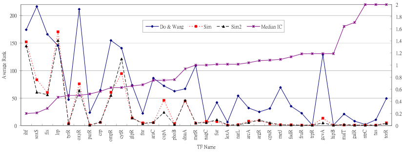
Figure 6: Comparison of three similarity measures using the 2-centroid method.

3.3 Yet another LOO CV

Two different sets of negative examples were used in the LOO CV experiments presented above since no prior knowledge of the test negatives was assumed. We now show that, with the knowledge of non-binding sites, a small representative set of negative examples can be found by a slightly different LOO CV procedure. To avoid ambiguity, we constantly refer to sets defined in Section 3.1.

Consider a particular TF with $n_{+}$ known TFBS’s of length $l$. Suppose that the goal is to search for sites to which this TF binds but avoid known binding sites of other TF’s. That is, the binding sites of the other 34 TF’s are assumed known. We first randomly sample a representative set of $10n_{+}$ l-mers, $N_{\text{rep}}$, from $N_{\text{test}}$ since $10n_{+}\approx 0.05|N_{\text{train}}|$. For each iteration of LOO CV, the test TFBS is left out. A scoring function is obtained using the $n_{+}-1$ training TFBS’s and $N_{\text{rep}}$. The rank of the test TFBS is then calculated based on its score and the scores of the non-TFBS’s in $N_{\text{test}}$. The average rank of this TF is computed at the end of the LOO CV procedure. A good representative set of $10n_{+}$ negative examples can be found by repeating this LOO CV procedure multiple times.

We sampled a representative set of negative examples for each TF by repeating the LOO CV procedure 32 times. Fig. 7 compares average ranks resulted from the LOO CV procedure described in this section to those obtained in the first set of LOO CV experiments. Results of the first LOO CV procedure are marked with suffix “_1”, while those of the LOO CV experiments described in this section are marked with suffix “_2”. As expected, the average ranks obtained from the second set of LOO CV experiments are lower or comparable to those obtained from the first set. Looking at the medians of ODV_P_1 and ODV_P_2, it may appear that ODV_P_2 performed worse than ODV_P_1. However, a statistical test [23] indicates that overall ODV_P_2 has lower average ranks than ODV_P_1 ($p$-value: 0.06975).

Figure 7: Box plots of average ranks of the 35 TF’s. Each nucleotide or nucleotide pair is weighted by its information content.

3.4 ULPB versus other methods

Since the ungapped likelihood under positional background method was evaluated by Salama and Stekel [20] on a data set collected from RegulonDB, we conducted LOO CV experiments using the second data set described in Section 2.1. The methods compared to ULPB include the position-specific probability matrix (PSPM) method, the position-specific scoring matrix method with nucleotide pairs (PSSM_P), the 2-centroid method with nucleotide pairs (2-centroid_P) and the optimal discriminating vector with nucleotide pairs (ODV_P). PSPM was chosen because it was one of the methods compared in [20]. PSSM_P was included because it does not require non-TFBS’s and it is similar to ULPB in that nucleotide pairs are considered. ODV_P and 2-centroid_P were compared because they employ non-TFBS’s explicitly. Information content was not used in all the methods compared in this section.

The methods were evaluated under the same LOO CV framework described in Section 3.1. Overall performance of the compared methods is summarized in Fig. 8. The box plots show that overall PSPM gave the highest average ranks, which is consistent with the results reported in [20] that ULPB performed better than PSPM. In terms of median marked by the horizontal bar inside a box, ULPB appears to be worse than PSSM_P, 2-centroid_P and ODV_P. Fig. 9 shows performance of the 4 methods on individual TF’s. We can see that PSSM_P performed better than ULPB on 15 out of 26 TF’s and 2-centroid_P/ODV_P performed better than ULPB on 14 out of 26 TF’s. To gauge the significance of these observations, statistical tests [23] were performed on all the 6 pairs of methods. The results however only support that 2-centroid_P outperformed PSPM ($p$-value: 0.000722), ODV_P outperformed PSPM ($p$-value: 0.03344) and PSSM_P outperformed PSPM ($p$-value: 0.006476). The $p$-values of the other tests are all greater than 5%, the usual significance cut-off. Similar to Fig. 6, the relation between performance and median information content can be observed as well.

Figure 8: Box plots of average ranks of the 26 TF’s in the second data set.

Figure 9: Comparison of the PSPM, PSSM_P, ULPB, 2-centroid_P and ODV_P methods using the second data set.

4 Discussion

4.1 No best method for all TF’s

We have shown in the previous section that overall methods utilizing negative examples perform better than methods using only positive examples. One may be tempted to identify the method that gives the lowest average rank for all the TF’s. From the results of our LOO CV experiments, however, we found that there’s no combination of method and similarity measure that is optimal for all the TF’s in the data sets. That is, introducing pairs of nucleotide in similarity computation or incorporating non-binding sites lowers the average ranks for most of the TF’s but increases the average ranks for a few of them. Fig. 6 serves as an example. It shows that the similarity measure proposed by [18] gives the highest average ranks for most of the TF’s but is the best one among the three measures for TF lrp when the 2-centroid method is used. It also shows that $\mathrm{Sim2}$ yields lower average ranks than $\mathrm{Sim}$ except for a few TF’s such as cytR and fur when used along with the 2-centroid method. Therefore, instead of finding the combination of similarity measure and method that is optimal for all the TF’s. It is more reasonable and practical to search for the best combination of similarity measure and method for a particular TF of interest, which can be achieved by CV experiments.

4.2 Complexity of transcription factor binding sites

Results presented in Fig. 6 and 9 indicate correlation between the “complexity” of a TF and its median information content across nucleotides. Therefore, we attempted to establish the relationship between average rank and three factors: the length, number of known TFBS’s and median information content. The average ranks on the second data set produced by 2-centroid_P in Fig. 9 were linearly regressed [25] on the three factors. Aside from the intercept, only the median information content was found significant ($p$-value: $2.89\times 10^{-7}$). A simple linear regression was then performed to obtain the linear relationship between average rank and median information content. Fig. 10 shows a scatter plot of average rank versus median information content for the 26 TF’s in the second data set. The straight line represents the relationship between average rank and median information content found by simple linear regression. The median information content can be viewed as a measure of conservedness of binding sites of a TF. This reasonably implies that the binding sites of a TF are easier to predict when they are more conserved.

Figure 10: Linear relationship between average rank and median information content. The average ranks were obtained by running 2-centroid_P without weighting by information content on the second data set.

4.3 Properties of Investigated Methods

To reveal properties of methods, we performed pair-wise comparisons on some of the methods investigated in this work. Fig. 11 shows the pair-wise comparisons of centroid_P, PSSM_P, 2-centroid_P and ODV_P with information content on the first data set. For each pair of methods, the 35 TF’s were divided into two groups depending on the performance of the methods. We then looked for statistical difference between the two groups in terms of three factors, that is, the number of known TFBS’s, the median IC and the length of binding sites. The comparison between centroid_P and PSSM_P indicates that PSSM_P performs better than centroid_P on 21 TF’s, i.e., there are 21 TF’s in one group and 14 TF’s in the other. Moreover, when PSSM_P performs better, the median IC of a TF is on average 1.10095, which is significantly ($p$-value $<5\%$) greater than 0.74928, the average median IC of a TF when centroid_P performs better. Similar interpretations lead to additional comments as follows. 2-centroid_P requires significantly less known TFBS’s than PSSM_P. ODV_P performs better than PSSM_P or 2-centroid_P when a TF has higher median IC and shorter binding sites.

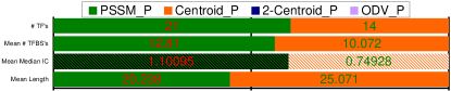
Figure 11: Pair-wise comparisons of centroid_P, PSSM_P, 2-centroid_P and ODV_P with information content on the first data set of 35 TF’s. Three factors except for # TF’s are tested for statistical significance. Significant factors are marked by striped bars.

Comparisons were also made between the four comparable methods, ODV_P, 2-centroid_P, PSSM_P and ULPB, on the second data set of 26 TF’s. Fig. 12 shows the bar plots. The plots suggest that 2-centroid_P performs better than PSSM_P when a TF has higher median IC and shorter binding sites. 2-centroid_P performs better than ODV_P when a TF has more known TFBS’s, ODV_P outperforms ULPB when a TF has less known TFBS’s and higher median IC, and ODV_P performs better than PSSM_P when a TF has less known TFBS’s.

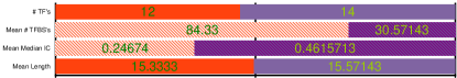
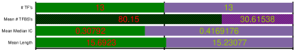
Figure 12: Pair-wise comparisons of ODV_P, 2-centroid_P, PSSM_P and ULPB without information content on the second data set of 26 TF’s. Three factors except for # TF’s are tested for statistical significance. Significant factors are marked by striped bars.

From the observations above, we can see that methods utilizing negative examples tend to perform better on TF’s with higher median information content. This suggests that the proposed 2-centroid and ODV methods are well-suited for identifying eukaryotic transcription factor binding sites. Fig. 13 shows the distribution of median IC of 459 eukaryotic transcription factors in the JASPAR database [26], where 75% (344 out of 459) of the TF’s have median IC above 1.02. According to our analysis shown in Fig. 11 and 12, the 2-centroid and ODV methods perform significantly better than other compared methods when a TF has relatively high median IC.

Figure 13: Distribution of median IC of 459 eukaryotic transcription factors in the JASPAR database.

Moreover, properties revealed in Fig. 11 and 12 can potentially help improve our 2-centroid and ODV methods. We can see in Fig. 10 that the median information content of a TF can be as low as 0.05. We suspect that the motif of such TF is actually a mixture of two or more motif subtypes, which contributes to its low median IC. We expect the motif subtypes of a TF to have higher median IC. Thus, a method can first identify motif subtypes contained in the known TFBS’s of a TF and then search for individual subtypes.

4.4 Motif Subtypes Improve the 2-centroid Method

It has been shown that the binding sites of a TF can be better represented by 2 motif subtypes than by a single motif [27, 28]. In search for new binding sites, two position-specific scoring matrices are used to score an $l$-mer and the higher score of the two is assigned to this $l$-mer. Searching with two PSSM’s was shown to be superior to searching with a single PSSM by cross-species conservation statistics in these studies.

To validate our hypothesis proposed in Section 4.3, we coupled motif subtypes with the centroid method as well as the 2-centroid method. Our approach to motif subtype identification is slightly different from those in previous work [27, 28], while the idea is similar. As usual, all the $l$-mers were first embedded in the Euclidean space as described in Section 2.2. The known binding sites of a TF were clustered into two subtypes by the $k$-means algorithm [29]. The centroids of these two subtypes, $\bm{\mu}_{+1}$ and $\bm{\mu}_{+2}$, were then computed. The centroid method coupled with motif subtypes is denoted by centroid_C and it scores an $l$-mer $t$ by

$$\max\left\{\bm{\mu}_{+1}^{\mathrm{T}}\bm{t},\bm{\mu}_{+2}^{\mathrm{T}}\bm{t}\right\},$$

where $\bm{t}$ denote the $l$-mer $t$ embedded in the Euclidean space. On the other hand, the 2-centroid method coupled with motif subtypes is denoted by 2-centroid_C and it score an $l$-mer $t$ by

$$\max\left\{\left(\bm{\mu}_{+1}-\bm{\mu}_{-}\right)^{\mathrm{T}}\bm{t},\left(\bm{\mu}_{+2}-\bm{\mu}_{-}\right)^{\mathrm{T}}\bm{t}\right\},$$

where $\bm{\mu}_{-}$ is the centroid of the non-binding sites.

We assessed and compared centroid_C and 2-centroid_C to their counterparts without motif subtypes by leave-one-out cross-validation on the second data set of 26 TF’s. Results summarized as box plots are shown in Fig. 14, where Pair denotes the use of nucleotide pairs and IC indicates weighting nucleotides and nucleotide pairs with information content. In all the four cases, significant improvement was observed when motif subtypes were taken into account. Table III elucidates the impact of motif subtype identification on our 2-centroid method. The first column shows that, before introducing motif subtypes, the improvement of 2-centroid over centroid is only statistically significant in the first row. The second column displays significant improvement of centroid_C over centroid, which was anticipated and consistent with the results reported in [27, 28]. The third column shows significant improvement of 2-centroid_C over 2-centroid in all four cases. We observed that the improvement of 2-centroid_C over 2-centroid is always more significant than the improvement of centroid_C over centroid. This implies that our 2-centroid method benefitted even more from the identification of motif subtypes. The last column indicates that, after the introduction of motif subtypes, 2-centroid_C significantly outperforms centroid_C in all cases. These results confirmed our hypothesis that, for TF’s with low median IC, methods employing non-binding sites should be coupled with motif subtype identification.

Figure 14: Box plots showing the LOO CV results of methods centroid, centroid_C, 2-centroid and 2-centroid_C. Pair denotes the use of nucleotide pairs and IC indicates weighting nucleotides and nucleotide pairs with information content.

TABLE III: Improvement by Identifying Motif Subtypes

		2-centroid $\rightarrow$ centroid		centroid_Ce $\rightarrow$ centroid		2-centroid_C $\rightarrow$ 2-centroid		2-centroid_C $\rightarrow$ centroid_C
Paira	ICb	# betterc	$p$-valued	# better	$p$-value	# better	$p$-value	# better	$p$-value
$\Box$	$\Box$	19	$2.793\times 10^{-2}$	18	$5.093\times 10^{-3}$	21	$2.205\times 10^{-5}$	21	$1.205\times 10^{-3}$
$\Box$	$\blacksquare$	18	$\bm{5.037\times 10^{-2}}$	19	$3.727\times 10^{-4}$	22	$1.135\times 10^{-5}$	19	$5.983\times 10^{-3}$
$\blacksquare$	$\Box$	17	$\bm{9.937\times 10^{-2}}$	16	$3.757\times 10^{-2}$	23	$6.661\times 10^{-6}$	18	$2.806\times 10^{-3}$
$\blacksquare$	$\blacksquare$	17	$\bm{1.185\times 10^{-1}}$	17	$7.003\times 10^{-3}$	20	$2.325\times 10^{-4}$	19	$8.807\times 10^{-3}$

• Whether a method uses nucleotide pairs.

• Whether a method weights nucleotide and nucleotide pairs with information content.

• The number of TF’s supporting the relationship being tested.

• $p$-value of the relationship produced by a statistical test [23].

• Suffix _C denotes coupling a method with motif subtypes.

Fig. 15 illustrates the application of 2-centroid_C with nucleotide pairs to transcription factor FlhDC in the second data set. It can be seen in Fig. 15a that the information content of FlhDC is low at all the 16 positions. After motif subtype identification, the two subtypes display distinct patterns and the information content of the two subtypes was greatly improved as seen in Fig. 15b. Fig. 15c shows a scatter plot of binding sites, non-binding sites and their respective centroids, while Fig. 15d shows a scatter plot of binding sites belonging to two subtypes, non-binding sites and their respective centroids after motif subtype identification. Many binding sites are not distinguishable from non-binding sites in Fig. 15c. However, after motif subtype identification, TFBS’s became separable from non-TFBS’s as seen in Fig. 15d, resulting in 1.7-fold improvement in average rank.

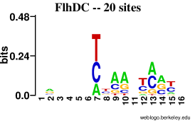
(a)

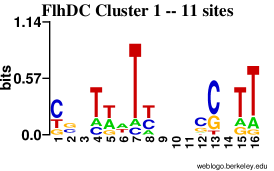
(b)

(c)

(d)

Figure 15: Illustration of the 2-centroid_C method with nucleotide pairs on transcription factor FlhDC in the second data set. Axes in (c) and (d) were found by Fisher’s discriminant analysis [30]. (a) Sequence logo before motif subtype identification. (b) Sequence logos of two motif subtypes identified by $k$-means clustering. (c) Scatter plot of binding sites, non-binding sites and their respective centroids, $\bm{\mu}_{+}$ and $\bm{\mu}_{-}$. The solid arrow identifies the vector $\bm{\mu}_{+}$, while the dashed arrow denotes the vector $\bm{\mu}_{+}-\bm{\mu}_{-}$. (d) Scatter plot of two clusters of binding sites, non-binding sites and their respective centroids, $\bm{\mu}_{+1},\bm{\mu}_{+2}$ and $\bm{\mu}_{-}$. The two solid arrows represent vectors $\bm{\mu}_{+1}$ and $\bm{\mu}_{+2}$, while the two dashed arrows denotes vectors $\bm{\mu}_{+1}-\bm{\mu}_{-}$ and $\bm{\mu}_{+2}-\bm{\mu}_{-}$.

4.5 Connection between ODV and PSSM/ULPB

Finally, we elucidate the relation between ODV and PSSM/ULPB. We first derive the connection between the optimal discriminating vector method and the position-specific scoring matrix method. Without loss of generality, we do not include nucleotide pairs in the derivation for simplicity reasons. We abuse notations for a moment and let $\beta_{i}(\text{A})=\beta_{4i-3}$, $\beta_{i}(\text{C})=\beta_{4i-2}$, $\beta_{i}(\text{G})=\beta_{4i-1}$ and $\beta_{i}(\text{T})=\beta_{4i}$. (7) then becomes

$$\bm{\beta}^{\mathrm{T}}\bm{t} =\sum_{i=1}^{l}\beta_{i}(t_{i})\sqrt{w_{i}}=\sum_{i=1}^{l}\log\left(\frac{f_{i}(t_{i})k_{i}}{f(t_{i})}\right)w_{i}$$

$$=\sum_{i=1}^{l}\log\left(\frac{f_{i}(t_{i})}{f(t_{i})}\right)w_{i}+\sum_{i=1}^{l}w_{i}\log k_{i},$$ (17)

where $f_{i}(t_{i})=\frac{1}{k_{i}}\exp\left(\frac{\beta_{i}(t_{i})}{\sqrt{w_{i}}}\right)f(t_{i})$ is the position-specific nucleotide frequency for $t_{i}$ induced by $\beta_{i}(\cdot)$ and

$$k_{i}=\sum_{u\in\{\text{A, C, G, T}\}}\exp\left(\frac{\beta_{i}(u)}{\sqrt{w_{i}}}\right)f(u)>0$$

is a scaling factor for position $i$ since ODV does not impose the constraints $\sum_{u\in\{\text{A, C, G, T}\}}f_{i}(u)=1,\,\,\forall i$. From (17), we note that $\sum_{i=1}^{l}w_{i}\log k_{i}$ does not depend on $t$ and thus $\bm{\beta}$ is optimal if and only if $\{f_{i}(u)|u\in\{\text{A, C, G, T}\}\text{ and }i=1,2,\ldots,l\}$, is optimal. Therefore, an optimal PSSM can be obtained from our ODV method.

The ungapped likelihood under positional background method is similar to the PSSM_P method in that both methods score nucleotides and nucleotide pairs. The ULPB method scores a $l$-mer $s$ by looking at the first nucleotide $s_{1}$ and all the $l-1$ adjacent nucleotide pairs $s_{1}s_{2},s_{2}s_{3},\ldots,s_{l-1}s_{l}$. Therefore, we can embed $s$ in $\mathbb{R}^{20l-16}$ by transforming $s_{1}$ into 4 dummy variables and each of the $l-1$ pairs into 16 dummy variables as described in Section 2.2. An optimal discriminating vector $\bm{\beta}\in\mathbb{R}^{20l-16}$ can then be found by applying our ODV method described in Section 2.3. Following similar arguments, we can see that there is a one-to-one correspondence between elements of $\bm{\beta}$ and $\left\{f_{1}(u),f_{i}(v|u)|u,v\in\{\text{A, C, G, T}\}\text{ and }i=1,2,\ldots,l-1\right\}$ in (15). Hence, an optimal ULPB can also be obtained from our ODV method.

One direct implication of the connection established above is that a vector obtained by the centroid, 2-centroid or ODV methods can be compared to a PSSM model in the same framework. As an example, Fig. 16 shows two sequence logos [31] of TF MalT in the second data set. The top logo represents the signature of the known binding sites, while the bottom one is obtained by converting the centroid $\bm{\mu}_{+}$ to a PSSM model as in (17) with $\bm{\beta}=\bm{\mu}_{+}$. The two logos display distinct patterns of the two methods, implying difference in performance. The PSSM method gave an average rank of 233.9, while the centroid method gave an average rank of 69.8. Clearly, the performance difference lies in the difference between the two logos. We can see that the two logos are very different at positions 3, 5, 6 and 10. Position 3 indicates that down-weighting letter T results in better performance. Position 10 shows that the influence of letter A is underestimated in the PSSM model. Other positions can be similarly compared and interpreted as well.

Figure 16: Two sequence logos of TF MalT. Top: PSSM; Bottom: centroid.

5 Conclusion

In this work, we investigated the use of negative examples in the TFBS search problem. To utilize negative examples, we proposed the 2-centroid and ODV methods, which are natural extensions of the centroid method. The proposed methods were compared to state-of-the-art methods relying purely on positive examples as well as a method considering negative examples. Comprehensive LOO CV results showed that non-TFBS’s are indeed helpful for TFBS search. The large number of non-binding sites can be significantly reduced by sampling a small representative set by LOO CV.

Not surprisingly, there is no single best TFBS search method or similarity measure for all the TF’s. The best combination of similarity measure and search method can be found for a particular TF by CV experiments. Nevertheless, pair-wise comparisons between methods revealed interesting properties of methods compared in this work. In particular, we showed that the 2-centroid and ODV methods are significantly better than the other methods when a TF has relatively high median information content. Even for TF’s with low median information content, preceded by motif subtype identification, the 2-centroid method was shown to be effective in searching for binding sites belonging to individual subtypes. The ODV method can be easily coupled with motif subtype identification as well and we believe significant improvement can be expected.

All the experiments in this work were conducted on prokaryotic transcription factors, i.e., TF’s in the E. coli K-12 genome. We claim that the proposed 2-centroid and ODV are well-suited for eukaryotic transcription factor binding site search as well. This is based on characteristics of the proposed methods and summary statistics of 459 eukaryotic transcription factors in the JASPAR database. Finally, we derived the connection between our ODV method and the PSSM method, showing that an optimal vector in ODV implies an optimal scoring matrix in PSSM and vice versa. Properly embedding an $l$-mer in an Euclidean space, the same connection between ODV and ULPB can be established as well.

The effects of negative examples on eukaryotic transcription factor binding site search will be investigated. Our future work also aims for extending our proposed methods to handling known binding sites of variable lengths. We will seek to approach this problem without resorting to multiple sequence alignment, which is notoriously time-consuming. In the meantime, we will also seek to identify better similarity measures than those investigated in this study.

Chih Lee

Chun-Hsi Huang

References

- [1] J. Vilo, A. Brazma, I. Jonassen, A. Robinson, and E. Ukkonen, “Mining for putative regulatory elements in the yeast genome using gene expression data,” in Proceedings of the Eighth International Conference on Intelligent Systems for Molecular Biology. AAAI Press, 2000, pp. 384–394.
- [2] Y. Barash, G. Bejerano, and N. Friedman, “A simple hyper-geometric approach for discovering putative transcription factor binding sites,” in WABI ’01: Proceedings of the First International Workshop on Algorithms in Bioinformatics. London, UK: Springer-Verlag, 2001, pp. 278–293.
- [3] J. Buhler and M. Tompa, “Finding motifs using random projections,” in RECOMB ’01: Proceedings of the fifth annual international conference on Computational biology. New York, NY, USA: ACM, 2001, pp. 69–76.
- [4] S. Sinha, “Discriminative motifs,” in RECOMB ’02: Proceedings of the sixth annual international conference on Computational biology. New York, NY, USA: ACM, 2002, pp. 291–298.
- [5] K. T. Takusagawa and D. K. Gifford, “Negative information for motif discovery,” in Pacific Symposium on Biocomputing. Pacific Symposium on Biocomputing, 2004, pp. 360–371.
- [6] S. Rajasekaran, S. Balla, and C.-H. Huang, “Exact algorithms for planted motif problems,” Journal of Computational Biology, vol. 12, no. 8, pp. 1117–1128, 2005.
- [7] S. Balla, V. Thapar, S. Verma, T. Luong, T. Faghri, C.-H. H. Huang, S. Rajasekaran, J. J. del Campo, J. H. Shinn, W. A. Mohler, M. W. Maciejewski, M. R. Gryk, B. Piccirillo, S. R. Schiller, and M. R. Schiller, “Minimotif miner: a tool for investigating protein function.” Nature methods, vol. 3, no. 3, pp. 175–177, March 2006. [Online]. Available: http://dx.doi.org/10.1038/nmeth856
- [8] N. Li and M. Tompa, “Analysis of computational approaches for motif discovery,” Algorithms for Molecular Biology, vol. 1, no. 1, p. 8, 2006. [Online]. Available: http://www.almob.org/content/1/1/8
- [9] E. Zaslavsky and M. Singh, “A combinatorial optimization approach for diverse motif finding applications,” Algorithms for Molecular Biology, vol. 1, no. 1, p. 13, 2006. [Online]. Available: http://www.almob.org/content/1/1/13
- [10] C. Yanover, M. Singh, and E. Zaslavsky, “M are better than one: an ensemble-based motif finder and its application to regulatory element prediction,” Bioinformatics, vol. 25, no. 7, pp. 868–874, 2009.
- [11] S. Georgiev, A. Boyle, K. Jayasurya, X. Ding, S. Mukherjee, and U. Ohler, “Evidence-ranked motif identification,” Genome Biology, vol. 11, no. 2, p. R19, 2010. [Online]. Available: http://genomebiology.com/2010/11/2/R19
- [12] M. Tompa, N. Li, T. L. Bailey, G. M. Church, B. De Moor, E. Eskin, A. V. Favorov, M. C. Frith, Y. Fu, W. J. Kent, V. J. Makeev, A. A. Mironov, W. S. S. Noble, G. Pavesi, G. Pesole, M. Régnier, N. Simonis, S. Sinha, G. Thijs, J. van Helden, M. Vandenbogaert, Z. Weng, C. Workman, C. Ye, and Z. Zhu, “Assessing computational tools for the discovery of transcription factor binding sites.” Nature biotechnology, vol. 23, no. 1, pp. 137–144, January 2005. [Online]. Available: http://dx.doi.org/10.1038/nbt1053
- [13] J. Hu, B. Li, and D. Kihara, “Limitations and potentials of current motif discovery algorithms,” Nucl. Acids Res., vol. 33, no. 15, pp. 4899–4913, 2005. [Online]. Available: http://nar.oxfordjournals.org/cgi/content/abstract/33/15/4899
- [14] G. Sandve and F. Drablos, “A survey of motif discovery methods in an integrated framework,” Biology Direct, vol. 1, no. 1, p. 11, 2006. [Online]. Available: http://www.biology-direct.com/content/1/1/11
- [15] R. Osada, E. Zaslavsky, and M. Singh, “Comparative analysis of methods for representing and searching for transcription factor binding sites,” Bioinformatics, vol. 20, no. 18, pp. 3516–3525, 2004.
- [16] G. Sandve, O. Abul, V. Walseng, and F. Drablos, “Improved benchmarks for computational motif discovery,” BMC Bioinformatics, vol. 8, no. 1, p. 193, 2007. [Online]. Available: http://www.biomedcentral.com/1471-2105/8/193
- [17] S. Hannenhalli, “Eukaryotic transcription factor binding sites–modeling and integrative search methods,” Bioinformatics, vol. 24, no. 11, pp. 1325–1331, 2008.
- [18] H. T. Do and D. Wang, “Overlap-based similarity metrics for motif search in dna sequences,” in ICONIP ’09: Proceedings of the 16th International Conference on Neural Information Processing. Berlin, Heidelberg: Springer-Verlag, 2009, pp. 465–474.
- [19] D. S. Chekmenev, C. Haid, and A. E. Kel, “P-Match: transcription factor binding site search by combining patterns and weight matrices,” Nucl. Acids Res., vol. 33, no. suppl_2, pp. W432–437, 2005.
- [20] R. A. Salama and D. J. Stekel, “Inclusion of neighboring base interdependencies substantially improves genome-wide prokaryotic transcription factor binding site prediction,” Nucl. Acids Res., vol. 38, no. 12, pp. e135–, 2010. [Online]. Available: http://nar.oxfordjournals.org/cgi/content/abstract/38/12/e135
- [21] J. Gregor, N. W. Davis, H. A. Kirkpatrick, M. A. Goeden, D. J. Rose, B. Mau, and Y. Shao, “The complete genome sequence of escherichia coli k-12.” Science, vol. 277, no. 5331, pp. 1453–1462, 1997.
- [22] S. Gama-Castro, V. Jiménez-Jacinto, M. Peralta-Gil, A. Santos-Zavaleta, M. I. Peñaloza-Spinola, B. Contreras-Moreira, J. Segura-Salazar, L. Muñiz-Rascado, I. Martínez-Flores, H. Salgado, C. Bonavides-Martínez, C. Abreu-Goodger, C. Rodríguez-Penagos, J. Miranda-Ríos, E. Morett, E. Merino, A. M. Huerta, L. Treviño-Quintanilla, and J. Collado-Vides, “RegulonDB (version 6.0): gene regulation model of Escherichia coli K-12 beyond transcription, active (experimental) annotated promoters and Textpresso navigation,” Nucleic Acids Research, vol. 36, no. suppl 1, pp. D120–D124, 2008.
- [23] F. Wilcoxon, “Individual comparisons by ranking methods,” Biometrics Bulletin, vol. 1, no. 6, pp. 80–83, 1945. [Online]. Available: http://dx.doi.org/10.2307/3001968
- [24] S. Holm, “A simple sequentially rejective multiple test procedure,” Scand J Statist, vol. 6, pp. 65–70, 1979.
- [25] N. Ravishanker and D. K. Dey, A First Course in Linear Model Theory. Chapman & Hall/CRC, December 2001.
- [26] J. C. Bryne, E. Valen, M.-H. E. Tang, T. Marstrand, O. Winther, I. da Piedade, A. Krogh, B. Lenhard, and A. Sandelin, “Jaspar, the open access database of transcription factor-binding profiles: new content and tools in the 2008 update,” Nucleic Acids Research, vol. 36, no. suppl 1, pp. D102–D106, 2008.
- [27] S. Hannenhalli and L.-S. Wang, “Enhanced position weight matrices using mixture models,” Bioinformatics, vol. 21, no. suppl_1, pp. i204–212, 2005.
- [28] B. Georgi and A. Schliep, “Context-specific independence mixture modeling for positional weight matrices,” Bioinformatics, vol. 22, no. 14, pp. e166–e173, 2006. [Online]. Available: http://bioinformatics.oxfordjournals.org/content/22/14/e166.abstract
- [29] M. J. de Hoon, S. Imoto, J. Nolan, and S. Miyano, “Open source clustering software.” Bioinformatics, vol. 20, no. 9, pp. 1453–1454, June 2004. [Online]. Available: http://dx.doi.org/10.1093/bioinformatics/bth078
- [30] T. Hastie, R. Tibshirani, and J. H. Friedman, The Elements of Statistical Learning (2nd edition). Springer, 2009.
- [31] G. E. Crooks, G. Hon, J.-M. Chandonia, and S. E. Brenner, “Weblogo: A sequence logo generator,” Genome Research, vol. 14, no. 6, pp. 1188–1190, June 2004. [Online]. Available: http://dx.doi.org/10.1101/gr.849004