Hedging bets with correlated quantum strategies

Abstract

This paper studies correlations among independently administered hypothetical tests of a simple interactive type, and demonstrates that correlations arising in quantum information theoretic variants of these tests can exhibit a striking non-classical behavior. When viewed in a game-theoretic setting, these correlations are suggestive of a perfect form of hedging, where the risk of a loss in one game of chance is perfectly offset by one’s actions in a second game. This type of perfect hedging is quantum in nature—it is not possible in classical variants of the tests we consider.

1 Introduction

It is well known that quantum information theory allows for correlations among measurement outcomes that are stronger than those possible within any classical theory. Bell inequality violations provide the archetypal example within this category, where space-like separated measurements of entangled particles yield correlated measurement outcomes that are incompatible with local hidden-variable theories [Bel64]. This paper describes a different scenario in which this phenomenon arises, and provides an example showing a striking difference between quantum and classical theories in this scenario.

We will begin with an abstract description of the scenario we consider that is mostly absent of precise discussions of underlying theories or mathematical structures. In simple terms, we imagine that one individual subjects another individual to a test, and for convenience we will refer to the individual administering the test as Alice and to the test-taker as Bob. One may of course envision that Alice and Bob are devices rather than individuals; we only choose the later point of view for the convenience of using the names Alice and Bob. The sort of tests under consideration are to have the following simple form:

• Alice prepares a question and sends it to Bob.

• Bob responds by sending an answer to Alice.

• Based on Bob’s answer, as well as whatever memory she has of her own question, Alice decides whether Bob has passed or failed the test.

In a purely classical setting, one may imagine that Alice’s behavior is described by a probabilistic process, whereby her questions are selected according to some probability distribution and her final decision might also involve the use of randomness. In the quantum setting, Alice’s questions may take the form of quantum information—possibly entangled with quantum memory of her own—and she may expect quantum information from Bob in return. In both the classical and quantum settings, we make the assumption that Bob has a complete description of the process by which Alice operates, and is generally interested in maximizing his probability of passing the test.

For a fixed choice for Alice’s test, let us let $p$ denote Bob’s optimal probability of passing. Formally speaking, without any assumptions on an underlying mathematical model, $p$ may be defined to be the supremum of all passing probabilities for Bob, taken over all possible choices of his strategy. (In both the classical and quantum models, the supremum will always be achieved, so that it may safely be replaced by the maximum.) By assumption, Alice always makes a definitive decision about whether Bob passes or fails, so he necessarily fails the test with probability at least $1-p$.

Now, consider that Alice instantiates two independent copies of her test: no correlations exist between the two questions that she presents to Bob, and the processes by which she determines whether Bob passes or fails are completely independent as well. There are a variety of questions that one may ask about this type of situation, including the following:

• What is the optimal probability with which Bob passes both tests?

• What is the optimal probability with which Bob passes at least one of the tests?

It is natural to guess that Bob’s optimal probability to pass both tests is $p^{2}$, while his optimal probability to pass at least one test is $1-(1-p)^{2}$. These are, of course, the optimal probabilities if he treats the two tests independently.

In the classical setting, the probabilities $p^{2}$ and $1-(1-p)^{2}$ are indeed optimal over all classical strategies, including those that do not respect the independence of the two tests; Bob cannot correlate the tests to his advantage in either case. While these claims can be proved directly with little difficulty, we will see that they fall out naturally as special cases in our analysis of the quantum setting.

In the quantum setting, the natural guess is indeed correct for the first question (as we will later discuss in greater detail): if Bob aims to pass both tests, there is no advantage for him to correlate the two tests. This fact is known to those that have studied quantum interactive proof systems [KW00], and it is a consequence of a more general result concerning semidefinite programs [MS07]. For the second question, on the other hand, the natural guess turns out to be wrong. We demonstrate this by giving an example where Bob can correlate the two independent tests in such a way that he passes at least one of the two tests with certainty, despite the fact that $p<1$. More specifically, our example describes a test where Bob’s optimal passing probability for a single instantiation of the test is $\cos^{2}(\pi/8)\approx 0.85$, while he never fails both tests if he correlates two independent instantiations in the right way.

Bob’s ability to correlate two independent tests in the way just described can be seen as a perfect form of hedging, as the following (highly fictitious) scenario illustrates. Bob is offered the opportunity to take part in two potentially lucrative but somewhat risky games of chance, run by Alice. The two games are completely independent and identical in nature: for each he must put forth $1 million of his own money to take part, and he has 85% chance to win if he plays optimally. For each game he wins, Bob receives $3 million (representing a $2 million gain over his initial $1 million investment), while he receives nothing (and loses his $1 million initial investment) if he loses. For the sake of this example, we are to consider that a $1 million or greater loss means ruin for Bob.

These are, of course, highly compelling games of chance, and many people would not hesitate to take out a $2 million loan to play both: the expected gain from each one is $1,550,000, and the chance for a loss in both, if they are treated independently, is only 2.25%. Bob, however, is a highly risk-averse person. While he would enjoy being a millionaire, he cannot accept a 2.25% chance of ruin. Classically speaking, Bob can do nothing to avoid at least a 2.25% chance of ruin, so he will choose not to play. If the two games are modeled by quantum information as in our example, however, Bob can be guaranteed a $1 million return, and can therefore play without fear: an appropriately chosen quantum strategy allows him to hedge his bets perfectly.

2 Preliminaries

We assume the reader to be familiar with the basics of quantum information theory, and suggest Nielsen and Chuang [NC00] to those who are not. The purpose of this section is to summarize some of the notation and basic concepts we make use of, and to highlight a couple of concepts that may be less familiar to some readers.

Basic notation, states, measurements and channels

For any finite-dimensional complex Hilbert space $\mathcal{X}$ we write $\mathrm{L}\left(\mathcal{X}\right)$ to denote the set of linear operators acting on $\mathcal{X}$, we write $\mathrm{Herm}\left(\mathcal{X}\right)$ to denote the set of Hermitian operators acting on $\mathcal{X}$, we write $\mathrm{Pos}\left(\mathcal{X}\right)$ to denote the set of positive semidefinite operators acting on $\mathcal{X}$, we write $\mathrm{Pd}\left(\mathcal{X}\right)$ to denote the set of positive definite operators acting on $\mathcal{X}$, and we write $\mathrm{D}\left(\mathcal{X}\right)$ to denote the set of density operators acting on $\mathcal{X}$. For Hermitian operators $A,B\in\mathrm{Herm}\left(\mathcal{X}\right)$ the notations $A\geq B$ and $B\leq A$ indicate that $A-B$ is positive semidefinite, and the notations $A>B$ and $B<A$ indicate that $A-B$ is positive definite.

Given operators $A,B\in\mathrm{L}\left(\mathcal{X}\right)$, one defines the inner product between $A$ and $B$ as $\left\langle A,B\right\rangle=\operatorname{Tr}(A^{\ast}B)$. For Hermitian operators $A,B\in\mathrm{Herm}\left(\mathcal{X}\right)$ it holds that $\left\langle A,B\right\rangle$ is a real number and satisfies $\left\langle A,B\right\rangle=\left\langle B,A\right\rangle$. For every choice of finite-dimensional complex Hilbert space $\mathcal{X}$ and $\mathcal{Y}$, and for a given linear mapping of the form $\Phi:\mathrm{L}\left(\mathcal{X}\right)\rightarrow\mathrm{L}\left(\mathcal{Y}\right)$, there is a unique mapping $\Phi^{\ast}:\mathrm{L}\left(\mathcal{Y}\right)\rightarrow\mathrm{L}\left(\mathcal{X}\right)$ (known as the adjoint of $\Phi$) that satisfies $\left\langle Y,\Phi(X)\right\rangle=\left\langle\Phi^{\ast}(Y),X\right\rangle$ for all $X\in\mathrm{L}\left(\mathcal{X}\right)$ and $Y\in\mathrm{L}\left(\mathcal{Y}\right)$.

A register is a hypothetical device that stores quantum information. Associated with a register $\mathsf{X}$ is a finite-dimensional complex Hilbert space $\mathcal{X}$, and each quantum state of $\mathsf{X}$ is described by a density operator $\rho\in\mathrm{D}\left(\mathcal{X}\right)$. Qubits are registers for which $\dim(\mathcal{X})=2$. A measurement of $\mathsf{X}$ is described by a set of positive semidefinite operators $\{P_{a}\,:\,a\in\Sigma\}\subset\mathrm{Pos}\left(\mathcal{X}\right)$, indexed by a finite non-empty set of measurement outcomes $\Sigma$, and satisfying the constraint $\sum_{a\in\Sigma}P_{a}=\mathbb{1}_{\mathcal{X}}$ (the identity operator on $\mathcal{X}$). If such a measurement is performed on $\mathsf{X}$ while it is in the state $\rho$, each outcome $a\in\Sigma$ results with probability $\left\langle P_{a},\rho\right\rangle$. A quantum channel is a completely positive and trace-preserving linear mapping of the form $\Phi:\mathrm{L}\left(\mathcal{X}\right)\rightarrow\mathrm{L}\left(\mathcal{Y}\right)$ that describes a hypothetical physical process that transforms each state $\rho$ of a register $\mathsf{X}$ into the state $\Phi(\rho)$ of another register $\mathsf{Y}$. The set of all channels of this form is denoted $\mathrm{C}\left(\mathcal{X},\mathcal{Y}\right)$. The identity channel that does nothing to a register $\mathsf{X}$ is denoted $\mathbb{1}_{\mathrm{L}\left(\mathcal{X}\right)}$.

The Hilbert space corresponding to a pair of registers $(\mathsf{X}_{1},\mathsf{X}_{2})$ is the tensor product $\mathcal{X}_{1}\otimes\mathcal{X}_{2}$ of the spaces corresponding to $\mathsf{X}_{1}$ and $\mathsf{X}_{2}$. Independent states, measurements and channels are represented by elementary tensors in the following straightforward way:

• If registers $\mathsf{X}_{1}$ and $\mathsf{X}_{2}$ are independently prepared in states $\rho_{1}$ and $\rho_{2}$, then the state of the pair $(\mathsf{X}_{1},\mathsf{X}_{2})$ is given by the density operator $\rho_{1}\otimes\rho_{2}$.

• If registers $\mathsf{X}_{1}$ and $\mathsf{X}_{2}$ are independently measured with respect to the measurements described by the collections $\{P_{a_{1}}\,:\,a_{1}\in\Sigma_{1}\}\subset\mathrm{Pos}\left(\mathcal{X}_{1}\right)$ and $\{P_{a_{2}}\,:\,a_{2}\in\Sigma_{2}\}\subset\mathrm{Pos}\left(\mathcal{X}_{2}\right)$, the resulting measurement on the pair $(\mathsf{X}_{1},\mathsf{X}_{2})$ is described by the collection $\{P_{(a_{1},a_{2})}\,:\,(a_{1},a_{2})\in\Sigma_{1}\times\Sigma_{2}\}$, where $P_{(a_{1},a_{2})}=P_{a_{1}}\otimes P_{a_{2}}\in\mathrm{Pos}\left(\mathcal{X}_{1}\otimes\mathcal{X}_{2}\right)$.

• If registers $\mathsf{X}_{1}$ and $\mathsf{X}_{2}$ are independently transformed into registers $\mathsf{Y}_{1}$ and $\mathsf{Y}_{2}$ according to the channels $\Phi_{1}\in\mathrm{C}\left(\mathcal{X}_{1},\mathcal{Y}_{1}\right)$ and $\Phi_{2}\in\mathrm{C}\left(\mathcal{X}_{2},\mathcal{Y}_{2}\right)$, respectively, then the transformation of the pair $(\mathsf{X}_{1},\mathsf{X}_{2})$ into the pair $(\mathsf{Y}_{1},\mathsf{Y}_{2})$ is described by the channel $\Phi_{1}\otimes\Phi_{2}\in\mathrm{C}\left(\mathcal{X}_{1}\otimes\mathcal{X}_{2},\mathcal{Y}_{1}\otimes\mathcal{Y}_{2}\right)$.

Linear mappings on operator spaces

Suppose $\operatorname{dim}(\mathcal{X})=n$ and assume that a standard orthonormal basis $\{\left|\mspace{0.5mu}1\mspace{0.5mu}\right\rangle,\ldots,\left|\mspace{0.5mu}n\mspace{0.5mu}\right\rangle\}$ of $\mathcal{X}$ has been selected. With respect to this basis, one defines the Choi-Jamiołkowski operator $J(\Phi)\in\mathrm{L}\left(\mathcal{Y}\otimes\mathcal{X}\right)$ of a linear mapping $\Phi:\mathrm{L}\left(\mathcal{X}\right)\rightarrow\mathrm{L}\left(\mathcal{Y}\right)$ as

$$J(\Phi)=\sum_{1\leq i,j\leq n}\Phi(\left|\mspace{0.5mu}i\mspace{0.5mu}\right\rangle\left\langle\mspace{0.5mu}j\mspace{0.5mu}\right|)\otimes\left|\mspace{0.5mu}i\mspace{0.5mu}\right\rangle\left\langle\mspace{0.5mu}j\mspace{0.5mu}\right|$$

The mapping $J$ is a linear bijection from the space of mappings of the form $\Phi:\mathrm{L}\left(\mathcal{X}\right)\rightarrow\mathrm{L}\left(\mathcal{Y}\right)$ to the operator space $\mathrm{L}\left(\mathcal{Y}\otimes\mathcal{X}\right)$. It is well-known that $\Phi$ is completely positive if and only if $J(\Phi)\in\mathrm{Pos}\left(\mathcal{Y}\otimes\mathcal{X}\right)$, and that $\Phi$ is trace-preserving if and only if $\operatorname{Tr}_{\mathcal{Y}}(J(\Phi))=\mathbb{1}_{\mathcal{X}}$ [Cho75, Jam72].

While the Choi-Jamiołkowski operator of a linear mapping $\Phi:\mathrm{L}\left(\mathcal{X}\right)\rightarrow\mathrm{L}\left(\mathcal{Y}\right)$ is most commonly considered when $\Phi$ is a channel, the concept is useful in more general settings (as is illustrated in [GW07] and [CDP09], for instance). The following lemma, whose proof makes use of the Choi-Jamiołkowski operator of a particular mapping, gives one technical example that will be useful later in the paper.

Lemma 1.

For every operator $A\in\mathrm{L}\left(\mathcal{X}\otimes\mathcal{Z}\right)$ there exists a mapping $\Psi_{A}:\mathrm{L}\left(\mathcal{Z}\right)\rightarrow\mathrm{L}\left(\mathcal{X}\right)$ that possesses the following property: for every mapping $\Phi:\mathrm{L}\left(\mathcal{X}\right)\rightarrow\mathrm{L}\left(\mathcal{Y}\right)$ and every operator $B\in\mathrm{L}\left(\mathcal{Y}\otimes\mathcal{Z}\right)$, the equation

$$\left\langle B,\left(\Phi\otimes\mathbb{1}_{\mathrm{L}\left(\mathcal{Z}\right)}\right)(A)\right\rangle=\left\langle\left(\mathbb{1}_{\mathrm{L}\left(\mathcal{Y}\right)}\otimes\Psi_{A}\right)(B),J(\Phi)\right\rangle$$

holds. Moreover, if $A$ is positive semidefinite, then $\Psi_{A}$ is completely positive.

Proof.

The unique mapping $\Psi_{A}:\mathrm{L}\left(\mathcal{Z}\right)\rightarrow\mathrm{L}\left(\mathcal{X}\right)$ for which $J(\Psi)=\overline{A}$ (the entry-wise complex conjugate of $A$) possesses the required property. This fact is easily verified for operators $A$ taking the form $A=\left|\mspace{0.5mu}i\mspace{0.5mu}\right\rangle\left\langle\mspace{0.5mu}j\mspace{0.5mu}\right|\otimes\left|\mspace{0.5mu}k\mspace{0.5mu}\right\rangle\left\langle\mspace{0.5mu}l\mspace{0.5mu}\right|$, in which case

$$\Psi_{A}(Z)=\left|\mspace{0.5mu}i\mspace{0.5mu}\right\rangle\!\left\langle\mspace{0.5mu}k\mspace{0.5mu}\right|\!Z\!\left|\mspace{0.5mu}l\mspace{0.5mu}\right\rangle\!\left\langle\mspace{0.5mu}j\mspace{0.5mu}\right|,$$

and it follows for general operators by the conjugate-linearity/linearity of the inner product. Under the assumption that $A$ is positive semidefinite, so too is $\overline{A}$, from which it follows that $\Psi_{A}$ is completely positive. ∎

Semidefinite programming

Semidefinite programming is a topic that has found several interesting applications within quantum computing and quantum information theory in recent years. It is a valuable analytic tool, as well as a computational one. Here, we provide just a brief summary of semidefinite programming that is focused on the narrow aspects of it that we use. More comprehensive discussions can be found in [VB96, Lov03, dK02, BV04], for instance.

A semidefinite program is a triple $(\Phi,A,B)$, where

• $\Phi:\mathrm{L}\left(\mathcal{X}\right)\rightarrow\mathrm{L}\left(\mathcal{Y}\right)$ is a Hermiticity-preserving linear mapping, and

• $A\in\mathrm{Herm}\left(\mathcal{X}\right)$ and $B\in\mathrm{Herm}\left(\mathcal{Y}\right)$ are Hermitian operators,

for some choice of finite-dimensional complex Hilbert spaces $\mathcal{X}$ and $\mathcal{Y}$. We associate with the triple $(\Phi,A,B)$ two optimization problems, called the primal and dual problems, as follows:

Primal problem

maximize: $$\left\langle A,X\right\rangle$$

subject to: $$\Phi(X)=B,$$

$$X\in\mathrm{Pos}\left(\mathcal{X}\right).$$

Dual problem

minimize: $$\left\langle B,Y\right\rangle$$

subject to: $$\Phi^{\ast}(Y)\geq A,$$

$$Y\in\mathrm{Herm}\left(\mathcal{Y}\right).$$

The optimal primal value of this semidefinite program is

$$\alpha=\sup\{\left\langle A,X\right\rangle\,:\,X\in\mathrm{Pos}\left(\mathcal{X}\right),\,\Phi(X)=B\}$$

and the optimal dual value is

$$\beta=\inf\{\left\langle B,Y\right\rangle\,:\,Y\in\mathrm{Herm}\left(\mathcal{Y}\right),\,\Phi^{\ast}(Y)\geq A\}.$$

(It is to be understood that the supremum over an empty set is $-\infty$ and the infimum over an empty set is $\infty$, so $\alpha$ and $\beta$ are well-defined values in the set $\mathbb{R}\cup\{-\infty,\infty\}$. Our interest, however, will only be with semidefinite programs for which $\alpha$ and $\beta$ are finite.)

It always holds that $\alpha\leq\beta$, which is a fact known as weak duality. The condition $\alpha=\beta$, which is known as strong duality, does not hold for every semidefinite program, but there are simple conditions known under which it does hold. The following theorem provides one such condition (that has both a primal and dual form).

Theorem 2 (Slater’s theorem for semidefinite programs).

Let $(\Phi,A,B)$ be a semidefinite program and let $\alpha$ and $\beta$ be its optimal primal and dual values.

• If $\beta$ is finite and there exists a positive definite operator $X\in\mathrm{Pd}\left(\mathcal{X}\right)$ for which $\Phi(X)=B$, then $\alpha=\beta$ and there exists an operator $Y\in\mathrm{Herm}\left(\mathcal{Y}\right)$ such that $\Phi^{\ast}(Y)\geq A$ and $\left\langle B,Y\right\rangle=\beta$.

• If $\alpha$ is finite and there exists a Hermitian operator $Y\in\mathrm{Herm}\left(\mathcal{Y}\right)$ for which $\Phi^{\ast}(Y)>A$, then $\alpha=\beta$ and there exists a positive semidefinite operator $X\in\mathrm{Pos}\left(\mathcal{X}\right)$ such that $\Phi(X)=B$ and $\left\langle A,X\right\rangle=\alpha$.

In words, the first item of this theorem states that if the dual problem is feasible and the primal problem is strictly feasible, then strong duality holds and the optimal dual solution is achievable. The second item is similar, with the roles of the primal and dual problems reversed.

3 Interactive measurements

We now discuss the scenario described in the introduction in greater mathematical detail, focusing on the quantum setting. As is to be expected, the classical setting may be seen as a special case of the quantum setting.

Tests of the form described in the introduction are modeled by interactive measurements, which are essentially measurements of quantum channels: an interactive measurement consists of a state preparation and a measurement, to be applied to a given quantum channel. More formally speaking, an interactive measurement is specified by three finite-dimensional complex Hilbert spaces $\mathcal{X}$, $\mathcal{Y}$ and $\mathcal{Z}$, along with two objects defined over these spaces:

• A state on the spaces $\mathcal{X}$ and $\mathcal{Z}$, represented by a density operator $\rho\in\mathrm{D}\left(\mathcal{X}\otimes\mathcal{Z}\right)$.

• A measurement $\{P_{a}\,:\,a\in\Sigma\}\subset\mathrm{Pos}\left(\mathcal{Y}\otimes\mathcal{Z}\right)$ on the spaces $\mathcal{Y}$ and $\mathcal{Z}$.

If such an interactive measurement is applied to a given channel $\Phi\in\mathrm{C}\left(\mathcal{X},\mathcal{Y}\right)$, the probability associated with each measurement outcome $a\in\Sigma$ is given by

$$p(a)=\left\langle P_{a},(\Phi\otimes\mathbb{1}_{\mathrm{L}\left(\mathcal{Z}\right)})(\rho)\right\rangle.$$

An interactive measurement of a channel $\Phi$ is illustrated in Figure 1.

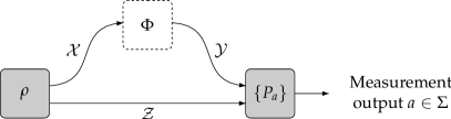
Figure 1: An interactive measurement, consisting of the preparation of a state $\rho\in\mathrm{D}\left(\mathcal{X}\otimes\mathcal{Z}\right)$ followed by a measurement $\{P_{a}\,:\,a\in\Sigma\}\subset\mathrm{Pos}\left(\mathcal{Y}\otimes\mathcal{Z}\right)$ on the space $\mathcal{Y}\otimes\mathcal{Z}$. The interactive measurement is applied to a given quantum channel $\Phi\in\mathrm{C}\left(\mathcal{X},\mathcal{Y}\right)$, which is illustrated by a dashed box in the figure.

Suppose that an interactive measurement, specified by a state $\rho\in\mathrm{D}\left(\mathcal{X}\otimes\mathcal{Z}\right)$ and a measurement $\{P_{a}\,:\,a\in\Sigma\}\subset\mathrm{Pos}\left(\mathcal{Y}\otimes\mathcal{Z}\right)$ has been fixed. For a given measurement outcome $a\in\Sigma$, one may consider both the maximum and minimum probability with which the outcome $a$ appears, over all choices of the quantum channel $\Phi$ upon which the interactive measurement is performed. Let us denote the maximum probability by $M(a)$ and the minimum probability by $m(a)$ for each $a\in\Sigma$, so that

$$M(a) =\max_{\Phi\in\mathrm{C}\left(\mathcal{X},\mathcal{Y}\right)}\left\langle P_{a},(\Phi\otimes\mathbb{1}_{\mathrm{L}\left(\mathcal{Z}\right)})(\rho)\right\rangle$$

$$m(a) =\min_{\Phi\in\mathrm{C}\left(\mathcal{X},\mathcal{Y}\right)}\left\langle P_{a},(\Phi\otimes\mathbb{1}_{\mathrm{L}\left(\mathcal{Z}\right)})(\rho)\right\rangle.$$

(One notes that the above quantities are the maximization and minimization, respectively, of a linear function on the compact set of quantum channels $\mathrm{C}\left(\mathcal{X},\mathcal{Y}\right)$. Thus, the use of the maximum and minimum rather than the supremum and infimum are justified.)

The quantities $M(a)$ and $m(a)$ are expressible as the optimal values of semidefinite programs, as we now describe. For each $a\in\Sigma$ we let $Q_{a}\in\mathrm{Pos}\left(\mathcal{Y}\otimes\mathcal{X}\right)$ be defined as

$$Q_{a}=\left(\mathbb{1}_{\mathrm{L}\left(\mathcal{Y}\right)}\otimes\Psi_{\rho}\right)(P_{a}),$$ (1)

for $\Psi_{\rho}$ being the mapping described by Lemma 1. We then have the following equality for each $a\in\Sigma$ and any choice of a channel $\Phi\in\mathrm{C}\left(\mathcal{X},\mathcal{Y}\right)$:

$$p(a)=\left\langle P_{a},(\Phi\otimes\mathbb{1}_{\mathrm{L}\left(\mathcal{Z}\right)})(\rho)\right\rangle=\left\langle Q_{a},J(\Phi)\right\rangle.$$

It therefore holds that

$$M(a)=\max_{\Phi\in\mathrm{C}\left(\mathcal{X},\mathcal{Y}\right)}\left\langle Q_{a},J(\Phi)\right\rangle\quad\quad\text{and}\quad\quad m(a)=\min_{\Phi\in\mathrm{C}\left(\mathcal{X},\mathcal{Y}\right)}\left\langle Q_{a},J(\Phi)\right\rangle.$$

The operator $J(\Phi)$ ranges over all choices of $X\in\mathrm{Pos}\left(\mathcal{Y}\otimes\mathcal{X}\right)$ satisfying $\operatorname{Tr}_{\mathcal{Y}}(X)=\mathbb{1}_{\mathcal{X}}$ as $\Phi$ ranges over all channels $\Phi\in\mathrm{C}\left(\mathcal{X},\mathcal{Y}\right)$, and therefore the following semidefinite program has optimal primal value $M(a)$:

Primal problem

maximize: $$\left\langle Q_{a},X\right\rangle$$

subject to: $$\operatorname{Tr}_{\mathcal{Y}}(X)=\mathbb{1}_{\mathcal{X}},$$

$$X\in\mathrm{Pos}\left(\mathcal{Y}\otimes\mathcal{X}\right).$$

Dual problem

minimize: $$\operatorname{Tr}(Y)$$

subject to: $$\mathbb{1}_{\mathcal{Y}}\otimes Y\geq Q_{a},$$

$$Y\in\mathrm{Herm}\left(\mathcal{X}\right).$$

A slight modification yields a semidefinite program whose optimal primal value is $m(a)$:

Primal problem

minimize: $$\left\langle Q_{a},X\right\rangle$$

subject to: $$\operatorname{Tr}_{\mathcal{Y}}(X)=\mathbb{1}_{\mathcal{X}},$$

$$X\in\mathrm{Pos}\left(\mathcal{Y}\otimes\mathcal{X}\right).$$

Dual problem

maximize: $$\operatorname{Tr}(Y)$$

subject to: $$\mathbb{1}_{\mathcal{Y}}\otimes Y\leq Q_{a},$$

$$Y\in\mathrm{Herm}\left(\mathcal{X}\right).$$

(The most straightforward way to fit this semidefinite program to the precise formalism described in Section 2 is to exchange maximums and minimums and replace $Q_{a}$ with $-Q_{a}$, which yields a semidefinite program for $-m(a)$. One could alternately extend the definition of semidefinite programs in a straightforward way to allow for minimizations in the primal problem and maximizations in the dual. The particular choice of these alternatives that one takes has no effect on our analysis.)

It is clear that strict feasibility holds for each of the problems presented: taking $X$ and $Y$ to be appropriately chosen scalar multiples of the identity operator suffices to observe that these properties hold. Strong duality therefore holds for both semidefinite programs by Theorem 2, and optimal solutions are achieved for each of the four problem formulations.

4 Correlations among independent interactive measurements

We now consider the situation in which two interactive measurements, described by pairs$\left(\rho_{1},\{P_{a_{1}}\,:\,a_{1}\in\Sigma_{1}\}\right)$ and $\left(\rho_{2},\{P_{a_{2}}\,:\,a_{2}\in\Sigma_{2}\}\right)$, are performed independently, as suggested in Figure 2.

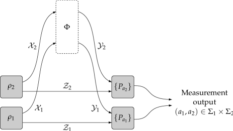
Figure 2: Two interactive measurements, specified by pairs $(\rho_{1},\{P_{a_{1}}\})$ and $(\rho_{2},\{P_{a_{2}}\})$, are performed independently. The two interactive measurements are applied to a channel $\Phi\in\mathrm{C}\left(\mathcal{X}_{1}\otimes\mathcal{X}_{2},\mathcal{Y}_{1}\otimes\mathcal{Y}_{2}\right)$, which may not respect the independence of the two interactive measurements, potentially causing a correlation in the two measurement outcomes.

While the interactive measurements are themselves performed independently, it is not assumed that the channel $\Phi\in\mathrm{C}\left(\mathcal{X}_{1}\otimes\mathcal{X}_{2},\mathcal{Y}_{1}\otimes\mathcal{Y}_{2}\right)$ respects this independence. Indeed, it is straightforward to devise examples where some choice of the channel $\Phi$ causes a correlation in the outcomes produced by the two measurements. The main focus of this section is on the nature of the correlations that are possible through the selection of various channels $\Phi$, especially as these correlations relate to the scenario described in Section 1.

Consider first the maximum output probability associated with a given pair of measurement outcomes $(a_{1},a_{2})\in\Sigma_{1}\times\Sigma_{2}$. In the following subsection we provide a proof that the maximum probability $M(a_{1},a_{2})$ with which this pair is output is given by

$$M(a_{1},a_{2})=M_{1}(a_{1})\,M_{2}(a_{2}),$$

where $M_{1}(a_{1})$ and $M_{2}(a_{2})$ denote the maximum output probabilities of $a_{1}$ and $a_{2}$ with respect to the individual interactive measurements with which they are associated. Thus, to maximize the probability of outputting $(a_{1},a_{2})$, there is absolutely no gain in choosing a channel $\Phi$ that correlates the two interactive measurements: the optimal probability is achieved by some choice $\Phi=\Phi_{1}\otimes\Phi_{2}$ that respects the independence of the two interactive measurements.

Remarkably, a similar property does not generally hold when the maximum is replaced by the minimum: we provide an example for which $m_{1}(a_{1})=m_{2}(a_{2})=\sin^{2}(\pi/8)\approx 0.15$, but $m(a_{1},a_{2})=0$.

Analysis for multiplicativity

To see that $M(a_{1},a_{2})=M_{1}(a_{1})M_{2}(a_{2})$, we may consider the semidefinite program representing the optimal probability $M(a_{1},a_{2})$:

Primal problem

maximize: $$\left\langle Q_{a_{1}}\otimes Q_{a_{2}},X\right\rangle$$

subject to: $$\operatorname{Tr}_{\mathcal{Y}_{1}\otimes\mathcal{Y}_{2}}(X)=\mathbb{1}_{\mathcal{X}_{1}\otimes\mathcal{X}_{2}},$$

$$X\in\mathrm{Pos}\left(\mathcal{Y}_{1}\otimes\mathcal{X}_{1}\otimes\mathcal{Y}_{2}\otimes\mathcal{X}_{2}\right).$$

Dual problem

minimize: $$\operatorname{Tr}(Y)$$

subject to: $$\pi(\mathbb{1}_{\mathcal{Y}_{1}}\otimes\mathbb{1}_{\mathcal{Y}_{2}}\otimes Y)\pi^{\ast}\geq Q_{a_{1}}\otimes Q_{a_{2}},$$

$$Y\in\mathrm{Herm}\left(\mathcal{X}_{1}\otimes\mathcal{X}_{2}\right).$$

(The unitary operator $\pi$ is defined by the action $\pi(y_{1}\otimes y_{2}\otimes x_{1}\otimes x_{2})=y_{1}\otimes x_{1}\otimes y_{2}\otimes x_{2}$ for all $y_{1}\in\mathcal{Y}_{1}$, $y_{2}\in\mathcal{Y}_{2}$, $x_{1}\in\mathcal{X}_{1}$, $x_{2}\in\mathcal{X}_{2}$.)

One first observes that the inequality $M(a_{1},a_{2})\geq M_{1}(a_{1})M_{2}(a_{2})$ is straightforward: the choice $X=X_{1}\otimes X_{2}$ for primal-optimal choices of $X_{1}$ and $X_{2}$ gives a primal feasible solution achieving the objective value $M_{1}(a_{1})M_{2}(a_{2})$.

Similarly, the upper bound $M(a_{1},a_{2})\leq M_{1}(a_{1})M_{2}(a_{2})$ may be established by considering the dual problem. For $Y_{1}\in\mathrm{Herm}\left(\mathcal{X}_{1}\right)$ and $Y_{2}\in\mathrm{Herm}\left(\mathcal{X}_{2}\right)$ being dual-optimal we have $\operatorname{Tr}(Y_{1})=M(a_{1})$ and $\operatorname{Tr}(Y_{2})=M(a_{2})$, and thus $\operatorname{Tr}(Y_{1}\otimes Y_{2})=M_{1}(a_{1})M_{2}(a_{2})$. Moreover, as $Q_{a_{1}}$ and $Q_{a_{2}}$ are positive semidefinite and the constrains $\mathbb{1}_{\mathcal{Y}_{1}}\otimes Y_{1}\geq Q_{a_{1}}$ and $\mathbb{1}_{\mathcal{Y}_{2}}\otimes Y_{2}\geq Q_{a_{2}}$ hold, it follows that $\mathbb{1}_{\mathcal{Y}_{1}}\otimes Y_{1}$ and $\mathbb{1}_{\mathcal{Y}_{2}}\otimes Y_{2}$ are positive semidefinite. Using the fact that $A\geq B$ and $C\geq D$ implies $A\otimes C\geq B\otimes D$ for any choice of positive semidefinite operators $A$, $B$, $C$ and $D$, we have

$$\pi(\mathbb{1}_{\mathcal{Y}_{1}}\otimes\mathbb{1}_{\mathcal{Y}_{2}}\otimes Y_{1}\otimes Y_{2})\pi^{-1}=(\mathbb{1}_{\mathcal{Y}_{1}}\otimes Y_{1})\otimes(\mathbb{1}_{\mathcal{Y}_{2}}\otimes Y_{2})\geq Q_{a_{1}}\otimes Q_{a_{2}}.$$

The operator $Y_{1}\otimes Y_{2}$ is therefore dual feasible, so it is established that $M(a_{1},a_{2})\leq M(a_{1})M(a_{2})$.

We note that this is a particular instance of a semidefinite program obeying the product rule considered by Mittal and Szegedy [MS07], where the argument just presented is applied to a more general class of semidefinite programs.

When the maximum is replaced by the minimum, however, the above argument breaks down. In this case, the semidefinite program whose optimal value is $m(a_{1},a_{2})$ takes the following form:

Primal problem

minimize: $$\left\langle Q_{a_{1}}\otimes Q_{a_{2}},X\right\rangle$$

subject to: $$\operatorname{Tr}_{\mathcal{Y}_{1}\otimes\mathcal{Y}_{2}}(X)=\mathbb{1}_{\mathcal{X}_{1}\otimes\mathcal{X}_{2}},$$

$$X\in\mathrm{Pos}\left(\mathcal{Y}_{1}\otimes\mathcal{X}_{1}\otimes\mathcal{Y}_{2}\otimes\mathcal{X}_{2}\right).$$

Dual problem

maximize: $$\operatorname{Tr}(Y)$$

subject to: $$\pi(\mathbb{1}_{\mathcal{Y}_{1}}\otimes\mathbb{1}_{\mathcal{Y}_{2}}\otimes Y)\pi^{\ast}\leq Q_{a_{1}}\otimes Q_{a_{2}},$$

$$Y\in\mathrm{Herm}\left(\mathcal{X}_{1}\otimes\mathcal{X}_{2}\right).$$

The upper-bound $m(a_{1},a_{2})\leq m_{1}(a_{1})\,m_{2}(a_{2})$ is easily established by once again taking $X=X_{1}\otimes X_{2}$ for primal optimal points $X_{1}$ and $X_{2}$. For the lower-bound

$$m(a_{1},a_{2})\stackrel{{\scriptstyle?}}{{\geq}}m_{1}(a_{1})\,m_{2}(a_{2}),$$

however, a problem arises: unlike the situation for the maximum, one may not conclude that the operators $\mathbb{1}_{\mathcal{Y}_{1}}\otimes Y_{1}$ and $\mathbb{1}_{\mathcal{Y}_{2}}\otimes Y_{2}$ are positive semidefinite for optimal dual solutions $Y_{1}$ and $Y_{2}$ (and indeed they may not be positive semidefinite in some cases). One may fail to prove that the operator $Y=Y_{1}\otimes Y_{2}$ is dual-feasible in this case, so that a lower-bound is not established.

An example showing non-classical behavior

We now present our example of a quantum test that allows for a strong correlation of the sort described in Section 1. The test is as follows:

• Alice prepares a pair of qubits $(\mathsf{X},\mathsf{Z})$ in the state

  $$u=\frac{1}{\sqrt{2}}\left|\mspace{0.5mu}00\mspace{0.5mu}\right\rangle+\frac{1}{\sqrt{2}}\left|\mspace{0.5mu}11\mspace{0.5mu}\right\rangle\in\mathcal{X}\otimes\mathcal{Z},$$

  and sends $\mathsf{X}$ to Bob.

• Bob applies any quantum channel he likes to $\mathsf{X}$, obtaining a qubit $\mathsf{Y}$ that he sends back to Alice. As a result of his action, the pair $(\mathsf{Y},\mathsf{Z})$ then has some particular state $\sigma\in\mathrm{D}\left(\mathcal{Y}\otimes\mathcal{Z}\right)$.

• Alice measures $(\mathsf{Y},\mathsf{Z})$ with respect to the projective measurement $\{P_{0},P_{1}\}$, where $P_{0}=\mathbb{1}-P_{1}$ and $P_{1}=vv^{\ast}$ for

  $$v=\cos(\pi/8)\left|\mspace{0.5mu}00\mspace{0.5mu}\right\rangle+\sin(\pi/8)\left|\mspace{0.5mu}11\mspace{0.5mu}\right\rangle.$$

  The outcome 1 is to be interpreted that Bob passes the test, while the outcome 0 means that he fails.

Now, if Bob can produce a given state $\sigma\in\mathrm{D}\left(\mathcal{Y}\otimes\mathcal{Z}\right)$ in step 2, it must hold that

$$\operatorname{Tr}_{\mathcal{Y}}(\sigma)=\operatorname{Tr}_{\mathcal{X}}(uu^{\ast})=\frac{1}{2}\mathbb{1}_{\mathcal{Z}};$$ (2)

no action that Bob performs on his registers can influence the state of Alice’s register. The probability that Alice obtains the outcome 1 is

$$\left\langle P_{1},\sigma\right\rangle=\operatorname{F}(vv^{\ast},\sigma)^{2},$$

where $\operatorname{F}(\cdot,\cdot)$ denotes the fidelity function and where the equality holds by virtue of the fact that $vv^{\ast}$ is pure. By the monotonicity of the fidelity function under partial tracing, we have

$$\operatorname{F}(vv^{\ast},\sigma)^{2}\leq\operatorname{F}\left(\operatorname{Tr}_{\mathcal{Y}}(vv^{\ast}),\operatorname{Tr}_{\mathcal{Y}}(\sigma)\right)^{2}=\operatorname{F}(Q,R)^{2}$$

for

$$Q=\begin{pmatrix}\cos^{2}(\pi/8)&0\\ 0&\sin^{2}(\pi/8)\end{pmatrix}\quad\quad\text{and}\quad\quad R=\begin{pmatrix}\frac{1}{2}&0\\ 0&\frac{1}{2}\end{pmatrix}.$$

By a direct calculation we determine

$$\operatorname{F}(Q,R)^{2}=\left\lVert\mspace{1.0mu}\sqrt{Q}\sqrt{R}\mspace{1.0mu}\right\rVert_{1}^{2}=\frac{1}{2}\left(\cos(\pi/8)+\sin(\pi/8)\right)^{2}=\cos^{2}(\pi/8).$$

Alice therefore outputs 1, indicating that Bob passes the test, with probability at most $\cos^{2}(\pi/8)\approx 0.85$.

Finally, for two instantiations of the test described above, we consider what happens when Bob applies the phase flip $\left|\mspace{0.5mu}00\mspace{0.5mu}\right\rangle\mapsto-\left|\mspace{0.5mu}00\mspace{0.5mu}\right\rangle$, $\left|\mspace{0.5mu}01\mspace{0.5mu}\right\rangle\mapsto\left|\mspace{0.5mu}01\mspace{0.5mu}\right\rangle$, $\left|\mspace{0.5mu}10\mspace{0.5mu}\right\rangle\mapsto\left|\mspace{0.5mu}10\mspace{0.5mu}\right\rangle$, $\left|\mspace{0.5mu}11\mspace{0.5mu}\right\rangle\mapsto\left|\mspace{0.5mu}11\mspace{0.5mu}\right\rangle$ on the two qubits he receives. Alice has prepared the state

$$\frac{1}{2}\left|\mspace{0.5mu}0000\mspace{0.5mu}\right\rangle+\frac{1}{2}\left|\mspace{0.5mu}0011\mspace{0.5mu}\right\rangle+\frac{1}{2}\left|\mspace{0.5mu}1100\mspace{0.5mu}\right\rangle+\frac{1}{2}\left|\mspace{0.5mu}1111\mspace{0.5mu}\right\rangle\in\mathcal{X}_{1}\otimes\mathcal{Z}_{1}\otimes\mathcal{X}_{2}\otimes\mathcal{Z}_{2},$$

and Bob’s phase flip transforms this state to

$$-\frac{1}{2}\left|\mspace{0.5mu}0000\mspace{0.5mu}\right\rangle+\frac{1}{2}\left|\mspace{0.5mu}0011\mspace{0.5mu}\right\rangle+\frac{1}{2}\left|\mspace{0.5mu}1100\mspace{0.5mu}\right\rangle+\frac{1}{2}\left|\mspace{0.5mu}1111\mspace{0.5mu}\right\rangle\in\mathcal{Y}_{1}\otimes\mathcal{Z}_{1}\otimes\mathcal{Y}_{2}\otimes\mathcal{Z}_{2}.$$

Writing

$$w=-\sin(\pi/8)\left|\mspace{0.5mu}00\mspace{0.5mu}\right\rangle+\cos(\pi/8)\left|\mspace{0.5mu}11\mspace{0.5mu}\right\rangle$$

we find that

$$-\frac{1}{2}\left|\mspace{0.5mu}0000\mspace{0.5mu}\right\rangle+\frac{1}{2}\left|\mspace{0.5mu}0011\mspace{0.5mu}\right\rangle+\frac{1}{2}\left|\mspace{0.5mu}1100\mspace{0.5mu}\right\rangle+\frac{1}{2}\left|\mspace{0.5mu}1111\mspace{0.5mu}\right\rangle=\frac{1}{\sqrt{2}}v\otimes w+\frac{1}{\sqrt{2}}w\otimes v.$$

When Alice measures this state with respect to the measurement $\{\Pi_{0},\Pi_{1}\}$, she obtains exactly one outcome 0 and one outcome 1. Thus, it holds that $m(0,0)=0$; Bob passes exactly one of the two tests with certainty.

Analysis for the classical setting

We now observe that the behavior exhibited in the example just described cannot happen in the classical setting.

Suppose that $\rho\in\mathrm{D}\left(\mathcal{X}\otimes\mathcal{Z}\right)$ and $\{P_{a}\,:\,a\in\Sigma\}\subset\mathrm{Pos}\left(\mathcal{Y}\otimes\mathcal{Z}\right)$ describe an interactive measurement as before. As is typical in quantum information theory, the classical setting corresponds to the special case in which these operators are all diagonal (with respect to the standard basis). Note that when the density operator $\rho$ and a given measurement operator $P_{a}$ are diagonal, it holds that the operator $Q_{a}\in\mathrm{Pos}\left(\mathcal{Y}\otimes\mathcal{X}\right)$ defined by (1) is also diagonal.

Now suppose that $a\in\Sigma$ is a measurement outcome for which $Q_{a}$ is diagonal, and consider the semidefinite program whose optimal primal value describes the minimum probability associated with the outcome $a$ (i.e., whose optimal value is $m(a)$):

Primal problem

minimize: $$\left\langle Q_{a},X\right\rangle$$

subject to: $$\operatorname{Tr}_{\mathcal{Y}}(X)=\mathbb{1}_{\mathcal{X}},$$

$$X\in\mathrm{Pos}\left(\mathcal{Y}\otimes\mathcal{X}\right).$$

Dual problem

maximize: $$\operatorname{Tr}(Y)$$

subject to: $$\mathbb{1}_{\mathcal{Y}}\otimes Y\leq Q_{a},$$

$$Y\in\mathrm{Herm}\left(\mathcal{X}\right).$$

We will observe that there exists a dual optimal solution $Y$ that is positive semidefinite. It will be helpful for this purpose to let $\Lambda_{\mathcal{X}}\in\mathrm{C}\left(\mathcal{X},\mathcal{X}\right)$ and $\Lambda_{\mathcal{Y}}\in\mathrm{C}\left(\mathcal{Y},\mathcal{Y}\right)$ denote the completely dephasing channels corresponding to $\mathcal{X}$ and $\mathcal{Y}$, respectively. More precisely, the mapping $\Lambda_{\mathcal{X}}$ is defined by

$$\Lambda_{\mathcal{X}}(\left|\mspace{0.5mu}i\mspace{0.5mu}\right\rangle\!\left\langle\mspace{0.5mu}j\mspace{0.5mu}\right|)=\left\{\begin{array}[]{ll}\left|\mspace{0.5mu}i\mspace{0.5mu}\right\rangle\!\left\langle\mspace{0.5mu}j\mspace{0.5mu}\right|&\text{if $i=j$}\\ 0&\text{if $i\not=j$}\end{array}\right.$$

for $1\leq i,j\leq n$, where $\{\left|\mspace{0.5mu}1\mspace{0.5mu}\right\rangle,\ldots,\left|\mspace{0.5mu}n\mspace{0.5mu}\right\rangle\}$ is the standard basis of $\mathcal{X}$, and $\Lambda_{\mathcal{Y}}$ is defined similarly with respect to the standard basis of $\mathcal{Y}$.

Now consider an arbitrary dual optimal solution $Y_{0}\in\mathrm{Herm}\left(\mathcal{X}\right)$. The mapping $\Lambda_{\mathcal{Y}}\otimes\Lambda_{\mathcal{X}}$ is completely positive, so the relation $\mathbb{1}_{\mathcal{Y}}\otimes Y_{0}\leq Q_{a}$ implies that

$$\mathbb{1}_{\mathcal{Y}}\otimes\Lambda_{\mathcal{X}}(Y_{0})=(\Lambda_{\mathcal{Y}}\otimes\Lambda_{\mathcal{X}})(\mathbb{1}_{\mathcal{Y}}\otimes Y_{0})\leq(\Lambda_{\mathcal{Y}}\otimes\Lambda_{\mathcal{X}})(Q_{a})=Q_{a}.$$

The diagonal operator $\Lambda_{\mathcal{X}}(Y_{0})$ is therefore dual feasible. As $\Lambda_{\mathcal{X}}$ preserves trace, $\Lambda_{\mathcal{X}}(Y_{0})$ achieves the same dual objective value as $Y_{0}$, and is therefore optimal as well. Finally, define

$$Y=\sum_{i=1}^{n}\max\{0,\,\left\langle\mspace{0.5mu}i\mspace{0.5mu}\right|\Lambda_{\mathcal{X}}(Y_{0})\left|\mspace{0.5mu}i\mspace{0.5mu}\right\rangle\}\left|\mspace{0.5mu}i\mspace{0.5mu}\right\rangle\!\left\langle\mspace{0.5mu}i\mspace{0.5mu}\right|.$$

In other words, $Y$ is obtained from $\Lambda_{\mathcal{X}}(Y_{0})$ by replacing each negative diagonal entry with 0. The inequality $\mathbb{1}_{\mathcal{Y}}\otimes Y\leq Q_{a}$ follows from the inequality $\mathbb{1}_{\mathcal{Y}}\otimes\Lambda_{\mathcal{X}}(Y_{0})\leq Q_{a}$ together with the observation that each diagonal entry of $Q_{a}$ is necessarily nonnegative (because $Q_{a}$ is positive semidefinite). As $\operatorname{Tr}(Y)\geq\operatorname{Tr}(\Lambda_{\mathcal{X}}(Y_{0}))=\operatorname{Tr}(Y_{0})$, it follows that $Y$ is also dual optimal. (The reality, of course, is that $Y=\Lambda_{\mathcal{X}}(Y_{0})$, for otherwise $\Lambda_{\mathcal{X}}(Y_{0})$ would not have been dual optimal.)

Finally, consider the situation in which two classical interactive measurements, described by pairs $\left(\rho_{1},\{P_{a_{1}}\,:\,a_{1}\in\Sigma_{1}\}\right)$ and $\left(\rho_{2},\{P_{a_{2}}\,:\,a_{2}\in\Sigma_{2}\}\right)$, are performed. One finds that the equality

$$m(a_{1},a_{2})=m_{1}(a_{1})\,m_{2}(a_{2})$$ (3)

considered before must now hold by an analysis similar to the one for the maximum output probability case: positive semidefinite optimal dual solutions exist for the semidefinite program described above for each operator $Q_{a_{1}}$ and $Q_{a_{2}}$, allowing for the straightforward construction of optimal primal and dual solutions to the semidefinite program whose optimal value is $m(a_{1},a_{2})$, thereby implying (3).

5 Conclusion

This paper has considered correlated strategies against independently administered hypothetical tests of a simple interactive type. It has been demonstrated that correlations arising in quantum information theoretic variants of these tests can exhibit a non-classical hedging type of behavior.

One may, of course, consider situations in which more than two independent tests are performed, where a variety of statistics may be of interest. For example, one may consider Bob’s optimal probability to pass some threshold number $t$ of some (possibly large) number $k$ of independently administered tests. Based on our results we know that a surprising behavior exists even for the case $t=1$ and $k=2$, and it would be interesting to investigate the possible asymptotic behaviors that can arise.

The work of this paper is motivated by the problem of error reduction through parallel repetition for quantum interactive proof systems. In complexity theory, hypothetical tests along the lines of those we have considered are often studied as a tool to classify computational problems, and the resulting model is known as the interactive proof system model [GMR89, BM88]. Interactive proof systems that allow for interactions consisting of multiple rounds are often considered, but for the sake of this discussion we will focus only on those interactive proof systems that consist of a single question followed by a response—or, in other words, those interactions that correspond to interactive measurements as we have considered them in this paper.

In the context of interactive proof systems, the individual we have called Alice is called the verifier and Bob is called the prover. The verifier’s computational ability is limited (usually to probabilistic or quantum polynomial time) while the prover’s computational ability is unrestricted. For each input string $x$ to a fixed decision problem $L$, the prover and verifier engage in an interaction wherein the prover attempts to convince (or prove to) the verifier that the string $x$ should be accepted as a yes-instance of the problem $L$. To say that such a system is valid for the problem $L$ means two things: one is that it must be possible for a prover to convince the verifier to accept with high probability if the input is truly a yes-instance of the problem, and the second is that the verifier must reject no-instances of the problem with high probability regardless of the prover’s actions. The first requirement is called the completeness condition, and is analogous to the condition in formal logic that true statements can be proved. The second condition is called the soundness condition, and is analogous to the condition that false statements cannot be proved.

Suppose now that a particular verifier has been specified (for a fixed decision problem $L$) so that the following conditions hold:

• For each yes-instance $x$ to $L$, it is possible for a prover to convince the verifier to accept with probability at least $\alpha$.

• For each no-instance $x$ to $L$, the verifier always rejects with probability at most $\beta$, regardless of the prover’s actions.

It may be, for instance, that $\alpha=1/2+\delta$ and $\beta=1/2-\delta$ for some small constant $\delta>0$. A more desirable situation is one in which $\alpha$ is replaced by $1-\varepsilon$ and $\beta$ is replaced by $\varepsilon$ for a small value of $\varepsilon$. The process of specifying a new verifier based on the original one that meets stronger completeness and soundness conditions, such as the ones just suggested, is called error reduction.

In a purely algorithmic situation, the natural way to reduce error is to gather statistics from multiple independent executions of a given algorithm. For instance, if an algorithm outputs a binary value that is correct (for worst-case inputs) with a probability of at least 2/3 on any single execution of the algorithm, it is straightforward to obtain a new algorithm with a very high probability of correctness: one simply runs the original algorithm independently many times and takes the majority value as the output. A natural adaptation of this idea to interactive proof systems is to define a new verifier that independently runs many instances of the test performed by the original verifier, and accepts if and only if some suitably chosen threshold number of these independent tests would have led the original verifier to acceptance. In the situation under consideration, one is to understand that it is important for the new verifier to run these independent tests in parallel (as opposed to requiring the prover to respond sequentially to the individual tests).

It is not obvious that this works in the context of interactive proof systems for precisely the reason that has been considered in this paper: a hypothetical prover that interacts with many independent executions of an interactive proof system need not respect the independence of these executions. Nevertheless, in the classical setting it has long been known that error reduction through parallel repetition followed by a threshold value computation works perfectly for (single-prover) interactive proof systems. To say that the reduction is perfect means that if $p$ is the optimal success probability for the original verifier, then the optimal probability to cause at least $t$ acceptances among $k$ independent executions of the original verifier is

$$\sum_{j=t}^{k}\binom{k}{j}p^{j}(1-p)^{k-j}.$$ (4)

In other words, a prover gains absolutely no advantage in trying to correlate the independent tests performed by the verifier.

In the quantum setting, however, it was not previously known if parallel repetition followed by a threshold value computation could allow for a perfect error reduction (or indeed any error reduction at all for certain values of $\alpha$ and $\beta$). Our results show that parallel repetition followed by a threshold value computation does not lead to a perfect reduction of error: substituting $k=2$, $t=1$ and $p=\cos^{2}(\pi/8)$ into (4) yields an upper bound of approximately $0.98$, which is violated by the strategy we described in the previous section (which achieves the value 1). We note that parallel repetition does work in the case of perfect completeness (i.e., $\alpha=1$), wherein the threshold value computation is replaced by the logical-and [KW00], and that there is a more complicated method for error reduction (based on a logical-and of majorities), which does allow for error reduction in the general case of the setting under consideration [JUW09].

Based on the semidefinite programming formalism we have described, it is possible to prove an upper bound of

$$\sum_{j=t}^{k}\binom{k}{j}p^{j}$$

on the probability for a quantum prover to cause at least $t$ acceptances among $k$ independent executions as considered above. Unfortunately this expression does not lead to a reduction of errors for a wide range of choices of $\alpha>\beta$. This bound yields a value larger than 1 in some situations, and when the value is smaller than 1 we do not know how closely it can be approached by a valid quantum strategy.

Acknowledgments

Abel Molina acknowledges support from QuantumWorks, MITACS, a Mike and Ophelia Lazaridis Graduate Fellowship and a David R. Cheriton Graduate Scholarship. John Watrous acknowledges support from NSERC, CIFAR, QuantumWorks and MITACS.

References

- [Bel64] J. Bell. On the Einstein-Podolsky-Rosen paradox. Physics, 1(3):195–200, 1964.
- [BM88] L. Babai and S. Moran. Arthur-Merlin games: a randomized proof system, and a hierarchy of complexity classes. Journal of Computer and System Sciences, 36(2):254–276, 1988.
- [BV04] S. Boyd and L. Vandenberghe. Convex Optimization. Cambridge University Press, 2004.
- [CDP09] G. Chiribella, G. D’Ariano, and P. Perinotti. Theoretical framework for quantum networks. Physical Review A, 80(2):022339, 2009.
- [Cho75] M.-D. Choi. Completely positive linear maps on complex matrices. Linear Algebra and Its Applications, 10(3):285–290, 1975.
- [dK02] E. de Klerk. Aspects of Semidefinite Programming – Interior Point Algorithms and Selected Applications, volume 65 of Applied Optimization. Kluwer Academic Publishers, Dordrecht, 2002.
- [GMR89] S. Goldwasser, S. Micali, and C. Rackoff. The knowledge complexity of interactive proof systems. SIAM Journal on Computing, 18(1):186–208, 1989.
- [GW07] G. Gutoski and J. Watrous. Toward a general theory of quantum games. In Proceedings of the 39th Annual ACM Symposium on Theory of Computing, pages 565–574, 2007.
- [Hol09] Thomas Holenstein. Parallel repetition: Simplifications and the no-signaling case. Theory of Computing, 5:141–172, 2009.
- [Jam72] A. Jamiołkowski. Linear transformations which preserve trace and positive semidefiniteness of operators. Reports on Mathematical Physics, 3(4):275–278, 1972.
- [JUW09] R. Jain, S. Upadhyay, and J. Watrous. Two-message quantum interactive proofs are in PSPACE. In Proceedings of the 50th Annual IEEE Symposium on Foundations of Computer Science, pages 534–543, 2009.
- [KW00] A. Kitaev and J. Watrous. Parallelization, amplification, and exponential time simulation of quantum interactive proof system. In Proceedings of the 32nd Annual ACM Symposium on Theory of Computing, pages 608–617, 2000.
- [Lov03] L. Lovász. Semidefinite programs and combinatorial optimization. Recent Advances in Algorithms and Combinatorics, 2003.
- [MS07] R. Mittal and M. Szegedy. Product rules in semidefinite programming. In Fundamentals of Computation Theory, volume 4639 of Lecture Notes in Computer Science, pages 435–445. Springer-Verlag, 2007.
- [NC00] M. A. Nielsen and I. L. Chuang. Quantum Computation and Quantum Information. Cambridge University Press, 2000.
- [Raz98] R. Raz. A parallel repetition theorem. SIAM Journal on Computing, 27(3):763–803, 1998.
- [Raz08] R. Raz. A counterexample to strong parallel repetition. In 49th Annual IEEE Symposium on Foundations of Computer Science, pages 369–373, 2008.
- [VB96] L. Vandenberghe and S. Boyd. Semidefinite programming. SIAM Review, 38(1):49–95, 1996.