PPAK Wide-field Integral Field Spectroscopy of NGC 628: II. Emission line abundance analysis

Abstract

In this second paper of the series, we present the 2-dimensional (2D) emission line abundance analysis of NGC 628, the largest object within the PPAK Integral Field Spectroscopy (IFS) Nearby Galaxies Survey: PINGS. We introduce the methodology applied to the 2D IFS data in order to extract and deal with large spectral samples, from which a 2D abundance analysis can be later performed. We obtain the most complete and reliable abundance gradient of the galaxy up-to-date, by using the largest number of spectroscopic points sampled in the galaxy, and by comparing the statistical significance of different strong-line metallicity indicators. We find features not previously reported for this galaxy that imply a multi-modality of the abundance gradient consistent with a nearly flat-distribution in the innermost regions of the galaxy, a steep negative gradient along the disc and a shallow gradient or nearly-constant metallicity beyond the optical edge of the galaxy. The N/O ratio seems to follow the same radial behaviour. We demonstrate that the observed dispersion in metallicity shows no systematic dependence with the spatial position, signal-to-noise or ionization conditions, implying that the scatter in abundance for a given radius is reflecting a true spatial physical variation of the oxygen content. Furthermore, by exploiting the 2D IFS data, we were able to construct the 2D metallicity structure of the galaxy, detecting regions of metal enhancement, and showing that they vary depending on the choice of the metallicity estimator. The analysis of axisymmetric variations in the disc of NGC 628 suggest that the physical conditions and the star formation history of different-symmetric regions of the galaxy have evolved in a different manner.

1 Introduction

Nebular emission lines from bright-individual H II regions have been, historically, the main tool at our disposal for the direct measurement of the gas-phase abundance at discrete spatial positions in low redshift galaxies. A good understanding on the distribution of the chemical abundance across the surface of nearby galaxies (or through the comparison between them) it is necessary in order to place observational-based constrains on theories of galactic chemical evolution, while at the same time, derive accurate star formation histories and obtain information on the stellar nucleosynthesis of normal spiral galaxies.

Several factors dictate the chemical evolution in a galaxy, including the primordial composition, the content and distribution of molecular and neutral gas, the star formation history (SFH), feedback, the transport and mixing of gas, the initial mass function (IMF), etc. All these ingredients contribute through a complex process to the evolutionary histories of the stars and the galaxies in general. Accurate measurements of the present chemical abundance constrain the different possible evolutionary scenarios, and thus the importance of determining the elemental composition in a global approach, among different galaxy types.

Previous spectroscopic studies have unveil some aspects of the complex processes at play between the chemical abundances of galaxies and their physical properties. Although these studies have been successful by determining important relationships, scaling laws and systematic patterns (e.g. luminosity-metallicity, mass-metallicity, and surface brightness vs. metallicity relations Skillman et al. 1989; Vila-Costas & Edmunds 1992; Zaritsky et al. 1994; Tremonti et al. 2004; effective yield vs. luminosity and circular velocity relations Garnett 2002; abundance gradients and the effective radius of disks Diaz 1989; systematic differences in the gas-phase abundance gradients between normal and barred spirals Zaritsky et al. 1994; Martin & Roy 1994; characteristic vs. integrated abundances Moustakas & Kennicutt 2006; etc.), they have been limited by the number of objects sampled, the number of H II regions observed and the coverage of these regions within the galaxy surface.

In order to tackle the problem of the 2D spectroscopic coverage of the whole galaxy surface, we devised the PPAK Integral-field-spectroscopy Nearby Galaxies Survey: PINGS (Rosales-Ortega et al., 2010, hereafter Ros10), an IFS survey of nearby ($<$ 100 Mpc) well-resolved spiral galaxies. PINGS was specially designed to obtain complete maps of the emission-line abundances, stellar populations, and reddening using an IFS mosaicking imaging, which takes advantage of what is currently one of the world’s widest field-of-view (FOV) integral field unit (IFU).

NGC 628 (Messier 74) is a close, bright, grand-design spiral galaxy which has been extensively studied. With a projected optical size of 10.5 $\times$ 9.5 arcmin, it is the most extended object of the PINGS sample (see Table 1). With such dimensions, this galaxy allow us to study the 2D metallicity structure of the disk and the second order properties of its abundance distribution. In the first paper of this series (Sánchez et al., 2011, hereafter Paper I), we present a study of the line emission and stellar continuum of NGC 628 by means of pixel-resolved maps across the disk of the galaxy. This study included a qualitative description of the 2D distribution of the physical properties inferred from the line intensity maps, and a comparison of these properties with both the integrated spectrum of the galaxy and the spatially resolved spectra. In this second article, we present a detailed, spatially-resolved spectroscopic abundance analysis, based on different spectral samples extracted from the area covered by the IFS observations of NGC 628. Particular attention is paid to the spectra selection technique, considering several quality factors and performing sanity check tests to the different methods employed, after which we define a spectra selection methodology specially conceived for the study of the nebular emission in this galaxy, with a potential application to any IFU-based spectroscopic observation. This allow us to investigate the small and intermediate scale-size variation in line emission, and to derive the gas chemistry distribution across the surface of the galaxy with unprecedented detail.

The paper is organised as follows: In Section 2 we give an overview of the observations and data reduction, including a description of the technique implemented in order to decouple the nebular emission from the observed spectra. In Section 3 we introduce the methodology applied to the IFS data in order to extract distinct spectral samples from which a 2D abundance analysis can be performed. Diagnostic diagrams and radial trends of different physical parameters are derived in these section, comparing the results between the different sets of IFS data, and with previously published results, when appropriate. In Section 4 we perform an abundance analysis based on the spectra samples extracted in the previous section, obtaining the abundance gradient of the galaxy, comparing different strong-line metallicity indicators, and discussing their statistical significance. In Section 5 we explore variations on the nebular properties across the surface of the galaxy, related to geometrical and morphological features. Finally, in Section 6 we present a summary of the main results of the article.

2 Observations and data reduction

The PINGS observations for NGC 628 were carried out at the 3.5m telescope of the Calar Alto observatory with the Potsdam Multi Aperture Spectrograph, PMAS, (Roth et al., 2005) in the PPAK mode (Verheijen et al., 2004; Kelz et al., 2006). With a field-of-view of 74”$\times$65”, and a filling factor of $\sim$ 65%, PPAK is currently one of the widest IFU available worldwide. The PPAK fibre bundle consists of 331 science fibres of 2.7 arcsec diameter each, within a single hexagonal pattern. The sky background is sampled by 36 additional fibres, distributed in 6 bundles of 6 fibres each, positioned along a circle $\sim$ 90 arcsec from the center of the instrument FOV. Additionally, 15 fibres are used for internal calibration purposes.

Due to the large size of NGC 628 compared to the FOV of the instrument, a mosaicking scheme was adopted. The observations of the galaxy spanned a period of three-years (from 2006 to 2009), with a total of six observing nights and 34 different pointings. The central position was observed in dithering mode to gain spatial resolution, while the remaining 33 positions were observed without dithering due to the large size of the mosaic. The V300 grating was used for all the observations, covering the wavelength range $\sim$ 3700-7100 Å, with a spectral resolution of $FWHM\sim$ 8 Å. For the central position we obtained 2 exposures of 600 s for each dithering pointing, while for the rest of the tiles we collected 3 exposures of 600s per pointing. At least two different spectrophotometric stars per observing night were observed during the runs in order to perform flux calibration. In addition to the science pointings, sky exposures of 300s were taken each night in order to perform a proper subtraction of the sky contribution. Additional details on the observing strategy can be found in Ros10 and Paper I.

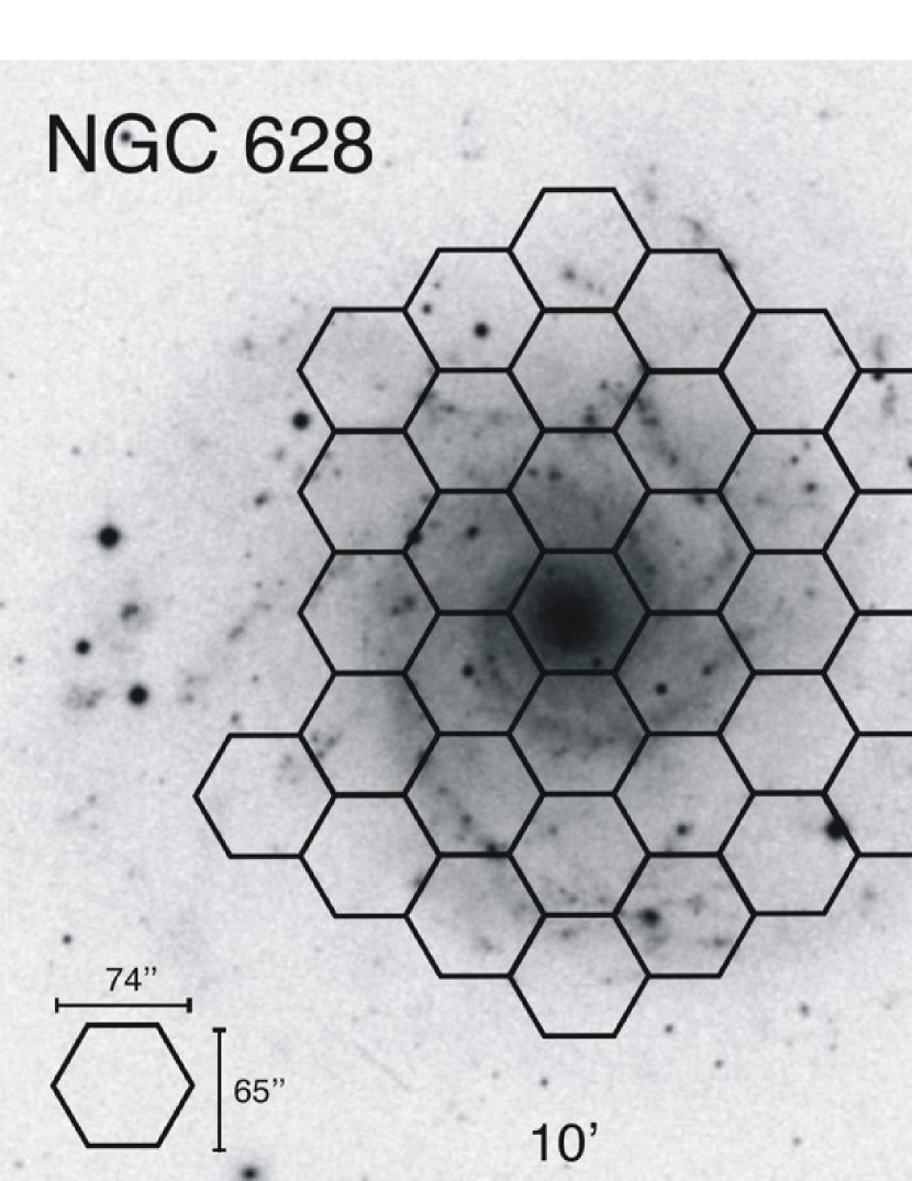
Figure 1: Area covered by the IFS observations of NGC 628. The figure shows a $B$-band Digital Sky Survey image of the galaxy with the PPAK mosaic pointings as overlaid hexagons indicating the field-of-view of the central fibre-bundle. The image is displayed in top-north, left-east standard configuration.

Fig. 1 displays a Digital Sky Survey image of NGC 628, showing the mosaic pattern covered by the IFS observations, consisting in a central position and consecutive hexagonal concentric rings. The spectroscopic mosaic contains 11094 individual spectra (considering overlapping and repeated exposures), the area covered by all the observed positions accounts approximately for 34 arcmin², making NGC 628 the largest area ever covered by a IFU mosaicking so far.

The reduction of the PINGS observations for NGC 628 followed, in general, the standard steps for fibre-based integral field spectroscopy. However, given that the observations of individual pointings were performed on different nights, during different years, with dissimilar atmospheric conditions, and slightly differing instrument configurations, the construction of the NGC 628 IFS mosaic required further reduction steps than for a single, standard IFU observation. The basic data reduction steps applied to the IFS mosaic of NGC 628 can be summarised as follows: a) Pre-reduction. b) Identification of the location of the spectra on the detector. c) Extraction of each individual spectrum. d) Distortion correction of the extracted spectra. e) Application of wavelength solution. f) Fibre-to-fibre transmission correction. g) Flux calibration. h) Allocation of the spectra to the sky position.

Data reduction was performed using r3d (Sánchez, 2006), in combination with iraf packages and e3d (Sánchez, 2004). A master bias frame was created by averaging all the bias frames observed during an observing night and subtracted from the science frames. The science exposures acquired at the same position on the sky were combined and the cosmic rays were removed during this process. The location of the spectra on the CCD were determined using a continuum illuminated exposure taken before the science exposures, each spectrum was then extracted from the science frames using an iterative Gaussian-suppression technique which reduces the effects of the cross-talk to negligible levels (Sánchez, 2006; Sánchez et al., 2011). The extracted flux for each spectrum was stored in a row-stacked-spectra (RSS) file (Sánchez, 2004). Wavelength calibration was performed using HeHgCd lamp exposures obtained before and after each pointing. Differences in the fibre-to-fibre transmission throughput were corrected by creating a master fibre-flat from twilight skyflat exposures taken in every run.

Sky-subtraction was then performed to the extracted, distortion/transmission corrected and wavelength calibrated spectra. Different sky subtraction schemes were applied depending on the location of the pointing within the IFS mosaic. By construction, in most of the NGC 628 pointings, the sky-fibres of the PPAK instrument are located within an area containing significant signal from the galaxy. In those cases, supplementary sky exposures were obtained applying large offsets from the observed positions. In some other cases, a sufficient number of sky-fibres were located in regions free from galaxy emission, where an accurate sky subtraction of the individual pointings using these sky spectra was possible. Relative flux calibration was attained by applying to the science frames a series of night sensitivity curves, obtained by comparing the observed flux with calibrated spectrophotometric standard spectra (reduced following the basic procedure described above), considering the filling factor of the fibre-bundle, corrections for the airmass and the optical extinction due to the atmosphere as a function of wavelength. In order to obtain the most accurate absolute spectrophotometric calibration, an additional correction was performed by comparing the IFS data with imaging photometry of the $B$, $V$, $R$ and H$\alpha$ images from the SINGS legacy survey (Kennicutt et al., 2003). The estimated spectrophotometric accuracy of the IFS mosaic is of the order of 0.2 mag. Furthermore, during this re-normalization process, the astrometry accuracy of the IFS mosaic was corrected to a $\sim$ 0.3 arcsec level. A complete explanation of the data processing and IFS mosaic creation is beyond the scope of this paper, but the reader will find a detailed description of the PINGS reduction process in Ros10, and in particular for the PPAK-IFS survey of NGC 628 in Paper I.

Table 1: Galaxy properties. Notes: (1) Morphological type from the R3C catalog (de Vaucouleurs et al., 1991). (2) Adopted distance in Mpc; Reference: Hendry et al. (2005). (3) Projected size, major and minor axes at the $B_{25}$ mag arcsec^-2 from R3C. (4) Absolute $B$-band magnitude calculated from the apparent magnitude listed in the R3C catalog and the adopted distance to the system. (5) Reference: Lu et al. (1993). (6) Heliocentric velocities calculated from $v=zc$, with no further correction applied. (7) Galaxy inclination angle based on the $B_{25}$ mag arcsec^-2 from R3C. (8) Galaxy position angle, measured positive NE, in the $B_{25}$ mag arcsec^-2. (9) Optical radius at the $B_{25}$ mag arcsec^-2 from R3C. (10) Optical radius in kpc assuming the adopted distance to the galaxy.

Property	NGC 628	Note
Type	SA(s)c	1
Adopted D (Mpc)	9.3	2
Projected size (arcmin)	10.5 $\times$ 9.5	3
$M_{B}$	-19.9	4
Redshift	0.00219	5
$V_{\odot}$ (km s-1)	657	6
Inclination $i$ (degrees)	24	7
P.A. (degrees)	25	8
$\rho_{25}$ (arcmin)	5.23	9
$\rho_{25}$ (kpc)	14.1	10

The final product of the reduction process for the IFS mosaic of NGC 628 consist in a RSS file containing 11094 wavelength and flux calibrated spectra, together with an ASCII position table file, which allocates each individual spectra to a sky position within the mosaic. However, many regions of the mosaic present a very low level of signal or do not contain signal at all (i.e. spectra with a flat continuum consistent with zero-flux intensity). The reason being that in those regions, the fibres were sampling areas where the intrinsic flux of the galaxy is low or null (e.g. borders of the mosaic, intra-arms regions, etc). In order to get rid of spectra where no information can be derived, we obtained a clean version of the IFS mosaic of NGC 628 by applying a flux threshold cut choosing only those fibres with an average flux along the whole spectral range greater than 10^-16 erg s^-1 cm^-2 Å^-1. Furthermore, bad fibres (due to cosmic rays and CCD cosmetic defects) and foreground stars (10 within the observed field-of-view of NGC 628) where removed from the mosaic. This procedure resulted in a refined mosaic version which includes only those regions with high-quality spectrophotometric calibration. The total number of spectra in the clean IFS mosaic version of NGC 628 is 6949.

The spectra of the clean mosaic of NGC 628 consist in a combination of continua arising from the different stellar populations, and emission of the ionized gas present in the interstellar medium of the galaxy. As the present study is focused on the spectroscopic properties of the gas-phase of NGC 628, the emission lines of the ionized gas were decouple from the stellar population in each individual spectrum of the IFS mosaic by using population synthesis to model and subtract the stellar continuum underlying the nebular emission lines. By applying this technique, the emission-line measurements are corrected (to a first-order) for stellar absorption. A thorough explanation of the stellar continuum fitting process (including a detailed description of the algorithms adopted, estimates of the accuracy of the SSP-based modeling and the derived parameters based on simulations) can be found in Paper I, here we only present a simplified scheme describing how the stellar populations and the emission lines in the IFS mosaic of NGC 628 were decoupled. First, a set of emission lines is identified from a strong H II region of the galaxy. For each spectrum in the data set, the underlying stellar population is fitted by a linear combination of a grid of Single Stellar Populations (SSP), after correcting for the appropriate systemic velocity and velocity dispersion, masking all the nebular and sky emission lines. The template models are selected in order to cover the widest possible range of ages and metallicities. We consider the effects of dust extinction by varying A_V from 0 to 1 mag at 0.2 mag steps. We subtract the fit stellar population from the original spectrum to get a residual pure emission-line spectrum.

A great deal of debate is found in the literature regarding the drawbacks of the SSP fitting technique discussed above, especially considering the well-known degeneracies found in the combination of SSPs (see Appendix of Paper I, and references therein). However, for this particular analysis, the only requirement is that that fit model can follow accurately the underlying continuum in order to decouple it from the emission lines produced by the ionized gas. Therefore, even in the case that the combination of SSPs is strongly degenerate, and the created model has no physical meaning, the latter can still be useful for this specific purpose. As a result of the SSP fitting procedure described before, we obtain two additional RSS files: one containing the continuum model fit to each individual spectra, and other containing the residual dataset of gas-free spectra.

Individual emission-line fluxes were measured in each spectrum of the residual RSS mosaic by considering spectral window regions of $\sim$ 200 Å. We performed a simultaneous multi-component fitting using a single Gaussian function (for each emission line contained within each window) plus a low order polynomial (to describe the local continuum and to simplify the fitting procedure) using fit3d (Sánchez et al., 2006). The central redshifted wavelengths of the emission lines were fixed and since the FWHM is dominated by the spectral resolution, the widths of all the lines were set equal to the width of the brightest line in this spectral region. Line intensity fluxes were then measured by integrating the observed intensity of each line. The statistical uncertainty in the measurement of the line flux was calculated by propagating the error associated to the multi-component fitting and considering the signal-to-noise of the spectral region.

The final result of all the procedures described above consist of a set of emission line intensities (and associated errors), per each of the 6949 individual spectra of the residual mosaic of NGC 628. The volume of this spectroscopic information is quite large, considering the classic view in which emission-line abundance studies were performed based on a few points across the surface of the galaxy. The following section describes the methodology implemented in order to extract meaningful information from this IFS database, which is then used to perform the 2D abundance analysis of NGC 628.

3 2D spectroscopic analysis of NGC 628

The nearly full IFS coverage of NGC 628 offers the possibility to undertake a detailed, spatially resolved, spectroscopic analysis of this galaxy based on thousands of individual spectra (within the limitation of the spatial resolution of the instrument). A spectroscopic analysis based on the emission line maps of NGC 628 is presented in Paper I, where the 2D distribution of the physical properties of the galaxy were studied. However, the conclusions raised from these maps are based on general trends and depend, to a certain level, on the interpolation scheme applied in order to derived the pixel-resolved maps.

Classical spectroscopy on this object has typically targeted a handful of bright individual H II regions in the galaxy (e.g. McCall et al., 1985; van Zee et al., 1998b; Ferguson et al., 1998; Castellanos et al., 2002), especially at the outer regions and along the spiral arms, where (in general) the contribution of the stellar population to the observed spectrum is not significant. However, the spectroscopic dataset presented in this series poses a challenge with respect to classical spectroscopy, as a right methodology has to be found in order to handle and analyse –in a homogeneous and meaningful way– this large spectroscopic database. In this section we consider two different spectra extraction techniques for the IFS analysis of NGC 628, they take into account the signal-to-noise of the data, the 2D spatial coverage, the physical sense of the derived results, and the final number of analysed spectra. In the first one, we consider all the fibres within the residual mosaic of the galaxy (i.e. using the maximum spatial resolution available), while in the second one we define “classical” H II regions by applying an aperture extraction on morphologically-linked emitting regions. A similar spectroscopic analysis is performed to both samples, a comparison of the results from the different analyses is also presented, together with an adopted final methodology.

3.1 Method I: fibre-by-fibre analysis

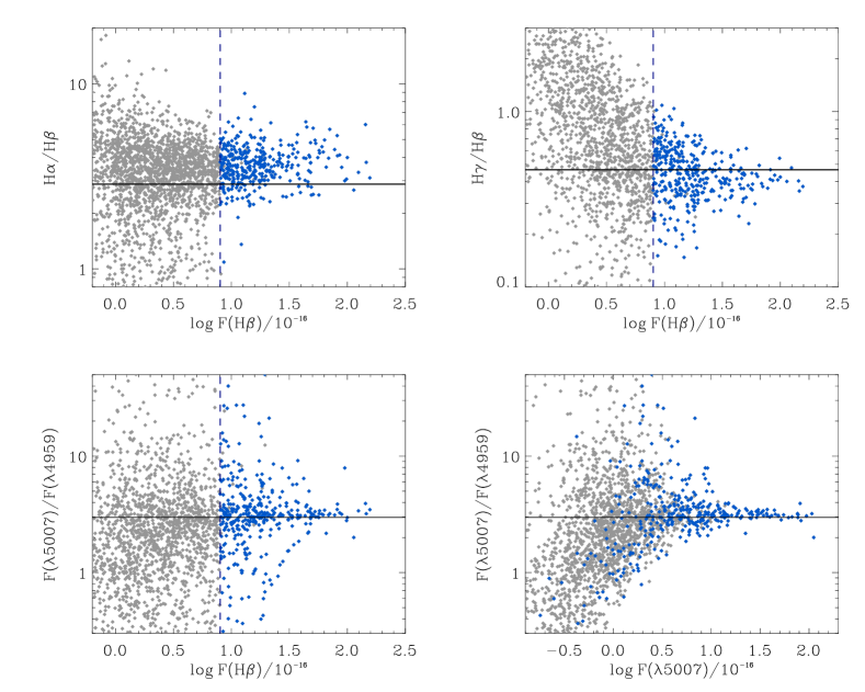
Figure 2: H$\alpha$/H$\beta$, H$\gamma$/H$\beta$ and [O III] $\lambda$5007/$\lambda$4959 ratios as a function of observed flux in H$\beta$ and F($\lambda$5007) for the fibre-by-fibre selection of NGC 628. Grey and blue symbols (in the online version) correspond to the diffuse and fibre-by-fibre samples, after the 2^nd (b) and 3^rd (c) selection criteria respectively, as described in the text. The horizontal lines correspond to the theoretical values for each ratio. The vertical dashed line stands for the flux threshold in H$\beta$.

The first of the explored analysis methods considers that the 2”.7 aperture of a single PPAK fibre would sample –in principle– a large-enough region in physical scale to subtend a small H II region and/or a fraction of a larger one at the adopted distance to the galaxy. With this assumption as a premise, the method considers every single fibre of the IFS mosaic as the source of an individual analysable spectrum. This method will be referred as the fibre-by-fibre analysis. In the case of NGC 628, at the assumed luminosity distance ($D_{\rm L}$ = 9.3 Mpc), one arcsec would correspond to a linear scale of $\sim$ 45 pc, assuming a standard $\Lambda$CDM cosmology (WMAP 5-years results: $H_{0}=70.5$, $\Omega=0.27$, $\Lambda=0.73$, Hinshaw et al. 2009). This linear physical scale implies that the fibre diameter of PPAK samples $\sim$120 pc on NGC 628, i.e. a region from which, in principle, one would expect enough signal-to-noise in the observed spectrum. This scale can be compared to the physical diameter of a well-known H II region in our Galaxy, i.e. the Orion nebula ($D\sim$ 8 pc), or to the extend of what are considered prototypes of extragalactic giant H II regions, such as 30 Doradus ($D\sim$ 200 pc) or NGC 604 ($D\sim$ 460 pc). Therefore, in the case of the fibre-by-fibre method, the area sampled by an individual fibre would subtend a fraction of a typical giant H II region in NGC 628, but the same area would fully encompass a number of small and medium size H II regions of the galaxy.

The spectra extraction process for the fibre-by-fibre method was based on the residual RSS file obtained after the clean mosaic version of the galaxy, as explained in Section 2. In the case of NGC 628, this mosaic corresponds to 6949 fibres, i.e. 51% of the total number of originally observed fibres. As it can be expected, not all the fibres in this mosaic have spectra with enough signal-to-noise and/or the right number of detectable emission lines in order to derive meaningful physical parameters. Following the experience of Paper I, we applied a flux threshold cut based on the H$\beta$ line intensity, together with some additional conditions. As the main focus is to characterise the chemical abundance of the galaxy, we required the presence in the spectrum of the typical emission lines from which we could carry out an abundance analysis in the individual fibres.

The sample selection was split in three different steps, the details of the criteria conditions in each step and their actual implementation in the IFS data can be found in Appendix A, they can be summarised as follows: a) We selected those fibres where the H$\beta$ and [O III] $\lambda$$\lambda$4959, 5007 emission lines were detected (i.e. line intensities greater than zero); b) We obtain a subsample based on the previous selection in which the logarithmic extinction coefficient c(H$\beta$) value (calculated from the H$\alpha$/H$\beta$ ratio, accordingly to the prescriptions describe in Paper I) was a finite-floating number, the total number of fibres fulfilling the two previous criteria was 2562, i.e. 37% of the fibres contained in the clean mosaic and 23% of the original number of fibres in the observed, unprocessed mosaic; c) Finally, we selected those fibres where the line intensity of the H$\beta$ line was greater than or equal to a given flux limit threshold, and the line intensity of [O II] $\lambda$3727 was greater than zero, i.e. the emission line was detected. The reasons for dividing the extraction procedure in these steps are explained in Appendix A, but the main intention was to extract data sets that could be analysed independently, as they could potentially trace regions of line emission with different physical properties, as explained thereinafter.

The value of the H$\beta$ flux threshold was chosen considering a trade-off between several factors: 1) The final number of spectra after the flux cut was applied; 2) The “quality” of the spectra as shown by certain line flux ratios and test diagrams (see below); and 3) The position of the derived spectra in some of the most common emission-line diagnostic diagrams. In the case of NGC 628, the flux limit applied in H$\beta$ was equal to 8 $\times$ 10^-16 erg s^-1 cm^-2. The final number of spectra in the fibre-by-fibre sample was 376 fibres, i.e. $\sim$ 6% of the number of fibres in the clean mosaic and $\sim$ 3% of the original fibres in the full NGC 628 mosaic.

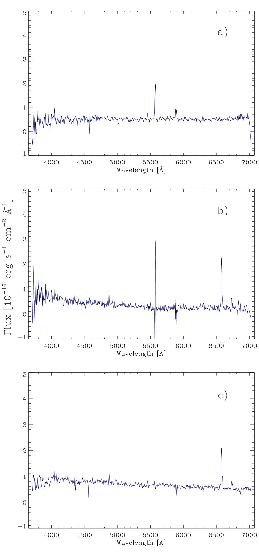
Figure 3: Examples of discarded spectra after the fibre-by-fibre selection criteria: a) spectrum without the presence of H$\beta$; b) spectrum with H$\alpha$, H$\beta$, but with low S/N and strong sky residuals; c) spectrum without [O II] $\lambda$3727.

A better understanding of the quality of the selected spectra can be inferred from Fig. 2. The top panels show the H$\alpha$/H$\beta$ and H$\gamma$/H$\beta$ ratios as a function of observed flux in H$\beta$, i.e. the variation of these ratios due to the intrinsic signal-to-noise of the data. The grey symbols correspond to the 2562 spectra selected after applying the selection criteria b) explained above, the blue symbols are overlaid on the previous data, showing the position of the selected spectra after the third selection criteria c) was applied, i.e. the final fibre-by-fibre sample. These two ratios correspond to the most important Balmer recombination ratios used to derive the reddening extinction in spectroscopic studies. Their values should be close to the theoretical ones (which depend mainly on the characteristic $T_{e}$) and, in high signal-to-noise spectra, the deviations from these values correspond to the effect of interstellar reddening, which tends to increase (H$\alpha$/H$\beta$) or decrease (H$\gamma$/H$\beta$) these ratios depending on the amount of extinction. For case-B recombination, and assuming a $T_{e}=10^{4}$ K, the theoretical values for the H$\alpha$/H$\beta$ and H$\gamma$/H$\beta$ ratios are 2.87 and 0.466 respectively (Table 4.2, Osterbrock & Ferland, 2006). The horizontal lines in each panel correspond to these theoretical values, while the vertical dashed lines correspond to the H$\beta$ flux threshold value.

For larger (observed) fluxes in H$\beta$, the scatter of the H$\alpha$/H$\beta$ and H$\gamma$/H$\beta$ ratios is smaller. As the signal-to-noise diminishes (exemplified here by the flux in H$\beta$), the scatter of the ratios increases to a considerable level. Ideally, in the case of the H$\alpha$/H$\beta$ ratio, a good signal-to-noise sample would be located above the theoretical line (consistent with physical reddening) and to the right of a certain flux limit. Conversely, in the case of the H$\gamma$/H$\beta$ ratio, an optimal sample would be located below the theoretical line and to the right of the flux ratio threshold. The value of the latter has to be chosen in order to find a good trade-off between the number of physically meaningful selected spectra, and the point at which the noise starts to dominate the measured ratios. As the H$\alpha$/H$\beta$ vs. log F(H$\beta$) diagram shows, the flux threshold is located exactly at the value when the scatter in the H$\alpha$/H$\beta$ ratio increases significantly for lower values of the H$\beta$ flux. A similar behaviour is found in the H$\gamma$/H$\beta$ diagram, although the scatter is in general higher, this would be expected as the H$\gamma$ line is more prone to measurement errors, due to its relatively low strength and because it is more affected by the correction for underlying absorption.

The bottom panels of Fig. 2 show the distribution of the [O III] $\lambda$5007/$\lambda$4959 ratio as a function of the observed flux in H$\beta$ (left) and of the observed flux in [O III] $\lambda$5007 (right). The ratio of the [O III] $\lambda$5007/$\lambda$4959 line strengths corresponds to the magnetic-dipole ${}^{1}D_{2}-^{3}P_{2}$ and ${}^{1}D_{2}-^{3}P_{1}$ transitions, which accordingly to theoretical work has a transition probability of 3.01, implying a fixed intensity ratio of 2.98 (Storey & Zeippen, 2000). Therefore, the line ratio of this [O III] doublet is an excellent indicator of the quality of the spectra of an ionized nebular region. The colour-coding (in the online version) is similar to the upper panels, the horizontal lines show the theoretical F($\lambda$5007)/F($\lambda$4959) ratio value. In both cases, an ideal spectroscopic sample would lie horizontally along the theoretical value over most of the intensity range, with a very small scatter around this value. The F($\lambda$5007)/F($\lambda$4959) vs. log F($\lambda$5007) plot shows this behaviour for a range of observed values log F($\lambda$5007) $\sim$ 1.0–2.0, for lower log F($\lambda$5007) values (i.e. lower signal-to-noise) the scatter increases considerably, even for the blue symbols corresponding to the final selected sample. In the case of the F($\lambda$5007)/F($\lambda$4959) vs. F(H$\beta$) diagram, most of the final selected sample lie near the theoretical value, however, a significant scatter in the F($\lambda$5007)/F($\lambda$4959) ratio is found even for relatively large H$\beta$ fluxes (i.e. higher signal-to-noise). The large dispersion found in the [O III] $\lambda$5007/$\lambda$4959 ratio might suggest that, despite the quality selection criteria and the low final number of extracted spectra, many of the selected fibres do not correspond to spectra of a “physical” emitting region. However, as it will be discussed below, the deviations of the [O III] ratio from the theoretical value are due to the effects introduced by subtraction of the stellar continuum in regions of weak oxygen emission.

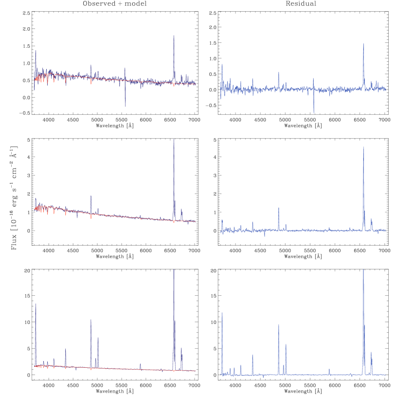
Figure 4: Examples of spectra with different S/N extracted from the final fibre-by-fibre sample. For each fibre, the left column corresponds to the observed spectrum, plus the SSP fit model overlaid as a red line, the right column shows the residual spectrum to which the selection criteria was later applied.

Fig. 3 shows examples of spectra discarded at different stages of the selection criteria, the top panel correspond to a spectrum of nearly null continuum, strong sky residuals and without signatures of H$\beta$ or any other important emission line, these sort of spectra were discarded after the first selection criterion. The rest of the panels show spectra with the signature of H$\alpha$ and H$\beta$ but strong sky residuals and low signal-to-noise (middle panel) or without the presence of the [O II] $\lambda$3727 line (bottom panel). These spectra were also discarded after the second and third selection criteria. On the other hand, Fig. 4 shows a series of three different individual fibres showing different ranges of signal-to-noise for the final selected fibre-by-fibre sample. For each fibre, the left column corresponds to the observed spectrum, plus the SSP fit model overlaid as a red line, the right column shows the residual spectrum to which the selection criteria was later applied. Note that all three spectra show the most important emission lines employed in the determination of metallicity using strong-line methods, i.e H$\alpha$, H$\beta$, [O II] $\lambda$3727, [O III] $\lambda$4959, [O III] $\lambda$5007, [N II] $\lambda$6548, [N II] $\lambda$6584, [S II] $\lambda$6717 and [S II] $\lambda$6731. Additionally, for those H II regions with high signal-to-noise we were able to detect and measure intrinsically fainter lines such as [Ne III] $\lambda$3869, H$\epsilon$ $\lambda$3970, H$\delta$ $\lambda$4101, H$\gamma$ $\lambda$4340, He I $\lambda$5876, [O I] $\lambda$6300, and He I $\lambda$6678 (e.g. see bottom panels of Fig. 4), although they have not been considered for the present study.

The line intensities of the final fibre-by-fibre sample were corrected by interstellar reddening using the c(H$\beta$) value together with the extinction law of Cardelli et al. (1989), assuming a total to selective extinction ratio $R=3.1$, following the same procedures as in Paper I. Formal errors were derived by propagating in quadrature the uncertainty in the flux calibration, the statistical error in the measurement of the line intensities and the error in the c(H$\beta$) term.

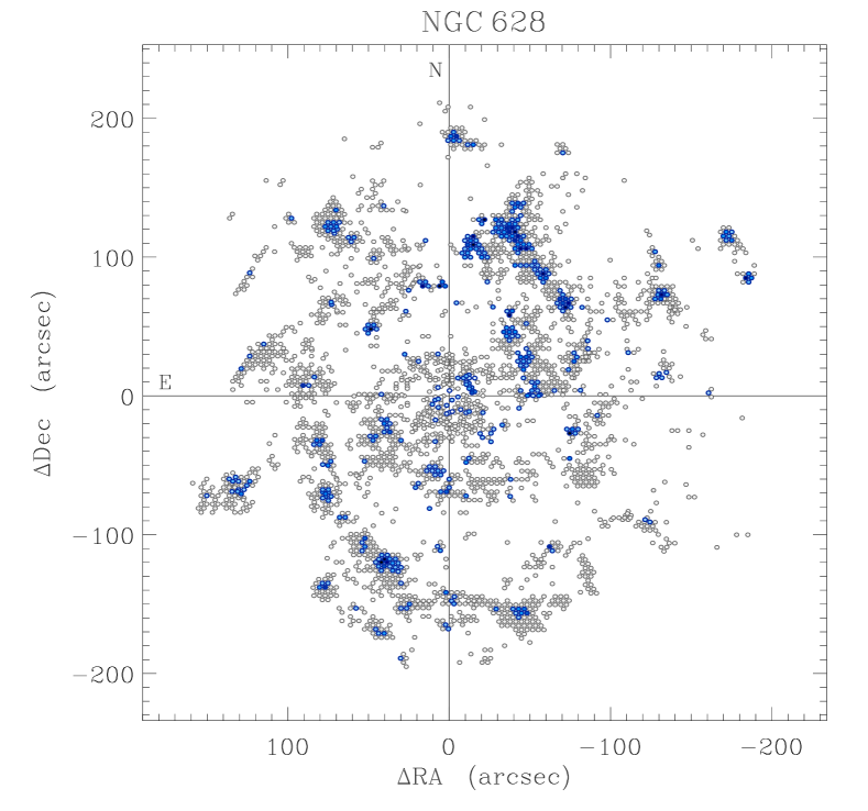
Figure 5: Spatial map of the fibre-by-fibre (blue) sample and the diffuse (grey) sample for NGC 628. The size and position of the fibres (at real scale) are displayed in the standard NE-positive orientation. The crosshairs mark the central reference point of the IFS mosaic. For the fibre-by-fibre sample, the colour intensity of each fibre has been scaled to the flux intensity of H$\alpha$ for that particular spectrum.

Fig. 5 shows the spatial positions of the different selected spectra, in a $\Delta$RA–$\Delta$Dec plane in the standard orientation (north-east positive), for the fibre-by-fibre analysis. The colour-coding is identical to Fig. 2, i.e. the grey fibres correspond to the subsample selected after the first and second selection criteria, the blue fibres are overlaid on the diagram, showing the position of the final selected sample after applying the third selection criteria. For the fibre-by-fibre sample (blue), the colour intensity of each fibre has been scaled to the flux intensity of H$\alpha$ for that particular spectrum. In that way, Fig. 5 would correspond to a H$\alpha$ emission line map obtained from the fibre-by-fibre data sample. The perpendicular lines intersect at the reference point of the IFS mosaic’s position table. A visual comparison with the interpolated H$\alpha$ emission line map of Paper I shows that the grey fibres correspond mainly to the edges of the H II regions and to regions of diffuse emission along the spiral arms and in the intra-arms regions. Some grey fibres are also found as isolated regions all over the surface of the mosaic. On the other hand, the blue fibres correspond mainly to the central areas of H II regions along the spiral arms, as well as some other bright sources over the surface of the galaxy. This behaviour would be expected, since the third selection criteria was based mainly on a H$\beta$ flux threshold, which separates the brightest fibres (i.e. the centre of H II regions) from the weaker ones, which correspond mainly to regions of diffuse emission. The fibres selected after the first and second selection criteria, corresponding to the grey fibres in Fig. 5, would be referred as the diffuse sample.

An additional way of studying the 2D distribution of the galaxy properties consists in obtaining azimuthally-averaged radial spectra, from which radial average properties can be derived. Taking the (blue) fibre-by-fibresample shown in Fig. 5 as a base, radial average spectra were obtained by co-adding all the spectra of this sample within successive rings of 10 arcsec, starting from the central reference point. An average spectrum was obtained for each single annulus at a given radius. Annulus with less than 5 fibres were excluded and skipped in the process. The radial average spectra were then analysed using the same fitting procedures described before. Although the derived spectra present more signal-to-noise than the single-fibre case, the measured emission lines were corrected by extinction using only the H$\alpha$/H$\beta$ ratio, for consistency with the fibre-by-fibre analysis.

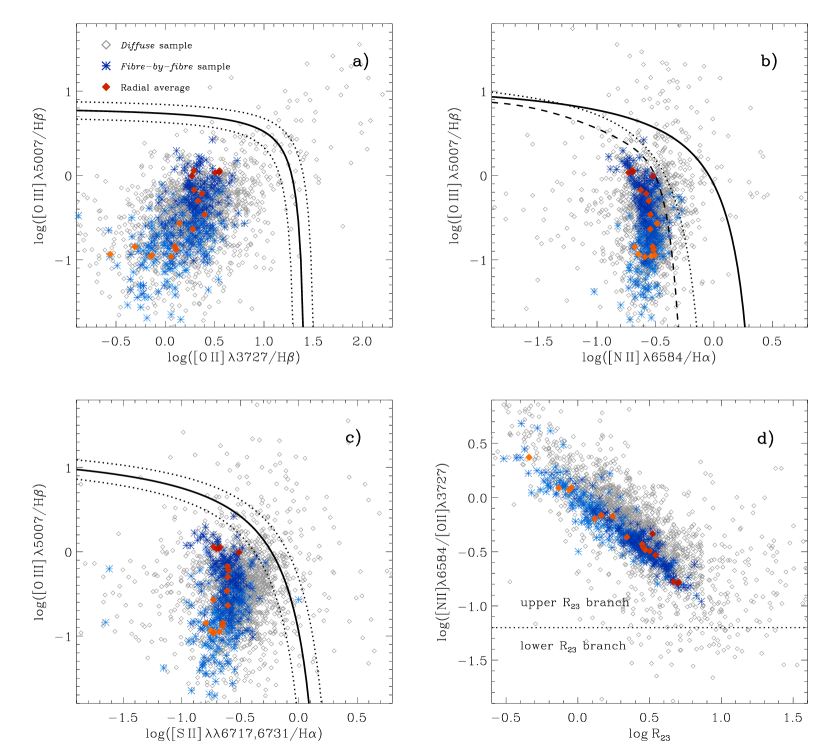
Figure 6: Diagnostic diagrams for NGC 628. The grey open diamonds correspond to the diffuse sample, the blue symbols to the final fibre-by-fibre sample and the filled diamonds to the azimuthally-averaged radial values. Lighter tones correspond to inner regions of the galaxy, darker colours to increasing galactocentric distance. The different lines correspond to the theoretical boundaries dividing star-forming regions from other types of ionization: Panel a) Lamareille et al. (2004); Panel b) dark-thick line: Kewley et al. (2001), dotted-line: Kauffmann et al. (2003), dashed-line: Stasińska et al. (2006); Panel c) and d) Kewley et al. (2001). In Panels a) and c) the dashed-lines represent the $\pm$0.1 dex variation.

Different possible mechanisms can be responsible for the ionization giving rise to emission line spectra in galaxies. The source driving the ionization in a given galaxy can be identified by exploring the location of certain line ratios in the so-called diagnostic diagrams (e.g. BPT, Baldwin et al., 1981; Veilleux & Osterbrock, 1987). These diagrams can be used as a tool to differentiate objects in which the photoionization is due by hot OB stars (H II regions), from objects in which is due to a non-thermal continuum (e.g. LINERs, AGNs) or to alternative mechanisms, such as the proposed retired galaxies, in which the ionization would be produced by hot post-asymptotic giant branch stars and white dwarfs (Stasińska et al., 2008). Fig. 6 shows a collection of different diagnostic diagrams for the spectral samples considered above, including the diffuse sample (grey open diamonds), the final fibre-by-fibre sample (bluish symbols), and the radial average sample (reddish diamonds). Panel a) corresponds to the classic BPT diagram [O III] $\lambda$5007/H$\beta$ vs. [O II] $\lambda$3727/H$\beta$, while panels b) and c) correspond to [O III] $\lambda$5007/H$\beta$ vs. [N II] $\lambda$6584/H$\alpha$ and vs. [S II] $\lambda$$\lambda$6717,31/H$\alpha$, respectively. Only those regions from the diffuse sample with detected [O II] $\lambda$3727 are drawn in Panels a) and d). The diagrams show different demarcation lines corresponding to the theoretical boundaries dividing the starburst region from other types of ionization. In Panel a) the delimitation is after Lamareille et al. (2004); in Panel b) the dark-thick line corresponds to the parametrization provided by Kewley et al. (2001), the dotted-line to Kauffmann et al. (2003), and the dashed-line to Stasińska et al. (2006); in Panel c) the demarcation is after Kewley et al. (2001). In Panels a) and c) the dashed-lines represent the $\pm$0.1 dex variation.

From these panels we see that the diffuse, low signal-to-noise spectra is scattered all over the diagrams, including those regions outside the boundaries which correspond to ionization sources different than OB stars. On the other hand, the line ratios corresponding to the fibre-by-fibre sample are encompassed by the theoretical H II regions boundaries. The line ratios of the radial averaged spectra are overlaid on each plot as filled diamonds. The colour-coding of both samples is related to the spatial position of a given fibre/annulus. Lighter tones correspond to the inner regions of the galaxy, while darker colours correspond to positions with increasing galactocentric radius. Clear trends can be noticed in each of the diagrams, in the case of Panel a) the spectra corresponding to the inner regions, both for the fibre-by-fibre and radial average sample, tend to have lower line ratios for both indices; for regions at the outer part of the galaxy, the ratios increase approaching the theoretical boundary. The reason for this behaviour can be understood from the emission line maps presented in Paper I, the inner parts of the galaxy lack emission in [O II] and [O III], while towards the outer parts, the emission from these species is prominent, increasing the two line ratios involved in this diagram. A slightly different trend is shown by the radial average spectra, which stay with a nearly constant [O III]/H$\beta$ value and increasing [O II]/H$\beta$ ratio, with increasing galactocentric distance up to [O II]/H$\beta$ $\sim$ 0.2, where the [O III]/H$\beta$ ratio increases considerably. In the case of Panels b) and c), the behaviour of both samples is quite similar. The [O III]/H$\beta$ ratio increases with galactocentric distance, but the [N II]/H$\alpha$ and [S II]/H$\alpha$ ratios do not vary much (except for some outlying blue fibres) and are concentrated along a vertical pattern centered at log [N II]/H$\alpha$ $\sim$ –0.6 and log [S II]/H$\alpha$ $\sim$ –0.7, with the [S II]/H$\alpha$ showing a slightly higher scatter. The radial average values follow the same trend in both cases, i.e. the azimuthally-average values of the [N II]/H$\alpha$ and [S II]/H$\alpha$ ratios do not change appreciably with increasing galactocentric distance. The locus of the fibre-by-fibre sample in all cases is consistent with regions in which the dominant ionization mechanism giving rise to the line emission of these spectra is a thermal continuum (i.e. hot OB stars). Therefore, the selection criteria applied in order to obtain the fibre-by-fibre sample did in fact extract those regions with spectra showing features of real H II regions.

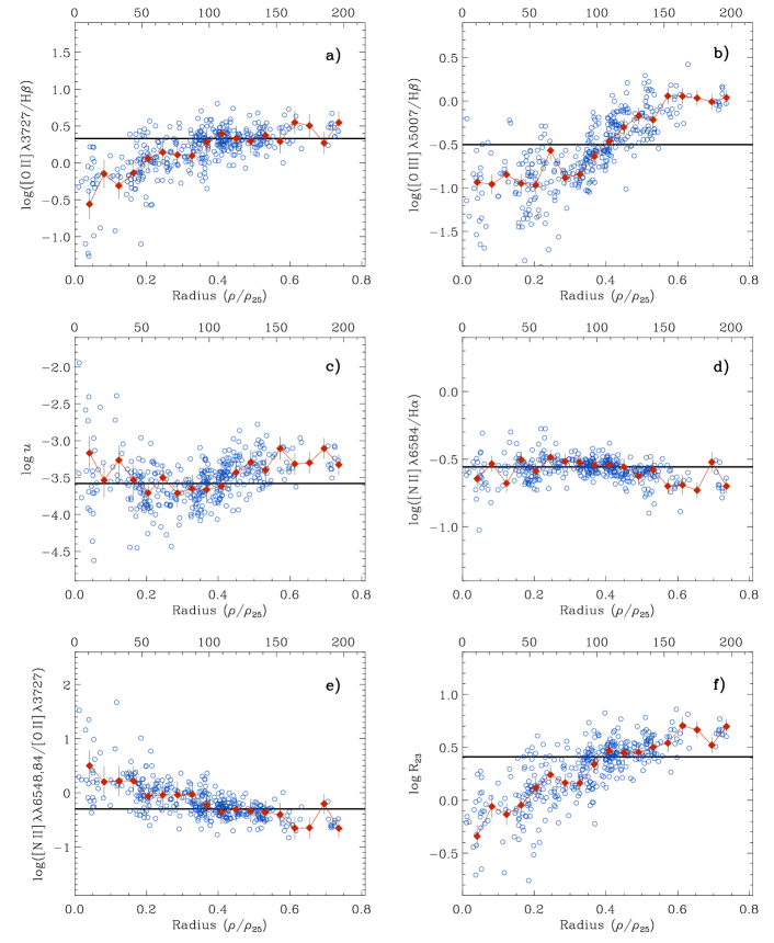
Figure 7: Radial variation of different line ratios and physical properties of NGC 628 for the fibre-by-fibresample (blue circles) and the azimuthally-averaged spectra (red diamonds). The deprojected radial position for the blue symbols has been normalised to the size of the optical disk at the 25 mag arcsec^-2 isophote. The radial position of the red diamonds correspond to the projected outer radius of the corresponding annulus. The top values on the $X$-axes show the linear-projected galactocentric radius in arcsec. The horizontal lines in each diagram correspond to the values derived from the integrated spectrum of NGC 628 presented in Paper I. Characteristic error bars are only drawn for the radial-averaged spectra for the sake of clarity.

The last panel of Fig. 6 corresponds to the [N II] $\lambda$6584/[O II] $\lambda$3727 vs. ([O II] $\lambda$3727 + [O III]$\lambda$4959,$\lambda$5007)/H$\beta$ (or $N_{2}O_{2}$ vs. $R_{23}$) diagnostic diagram. This is usually used to differentiate between the two branches of the $R_{23}$ abundance calibrator (Pagel et al., 1979) as explained in Paper I, and it is a strong function of metallicity for log [N II]/[O II] $\gtrsim$ –1.2 (Kewley & Dopita, 2002). As in the previous diagrams, the diffuse sample is spread over most regions of the plot, while the fibre-by-fibre sample and the radial average values are found along a well-defined pattern consistent with inner regions of the galaxy having higher $N_{2}O_{2}$ values and outer regions showing lower $N_{2}O_{2}$ ratios, which combined with the opposite behavior of $R_{23}$, create a correlation with a negative slope. All $N_{2}O_{2}$ values for the fibre-by-fibre sample correspond to the upper branch of the $R_{23}$ calibration, as implied in Paper I during the analysis of the emission line maps for this galaxy.

The radial trends of the line ratios inferred from Fig. 6 can be seen clearly in Fig. 7. Panel a) corresponds to the variation of [O II] $\lambda$3727/H$\beta$; Panel b) to [O III] $\lambda$5007/H$\beta$; Panel c) to the ionization parameter $\log u\equiv-0.80$ log([O II]/[O III]) $-3.02$, after Díaz et al. (2000); Panel d) to [N II] $\lambda$6584/[O II] $\lambda$3727; Panel e) to [S II] $\lambda$6717,31/H$\alpha$; and Panel f) to $R_{23}$. The blue circles correspond to the fibre-by-fibre spectra, while the red-connected diamonds correspond to the values derived from the radial averaged spectra. The deprojected radial position for the blue symbols has been normalised to the size of the optical disk at the 25 mag arcsec^-2 isophote. In each panel, the horizontal line corresponds to the value derived from the integrated spectrum of the galaxy in Paper I.

The [O II]/H$\beta$ and [O III]/H$\beta$ ratios on Panels a) and b) increase as a function of the radius, with a somewhat steeper increase for the [O III]/H$\beta$ ratio from a normalised radius $\sim$ 0.3, for lower radii this latter ratio shows some level of scatter, but consistent with a constant value log([O III]/H$\beta$) $\sim$ –1.0, as already noticed in Panel a) of the BPT diagrams shown in Fig. 6. The ionization parameter shows quite a lot of scatter for radii lower than 0.3$\rho_{25}$, due to the low strength of oxygen emission (from which this parameter is derived) in these inner regions. From $\rho/\rho_{25}>0.3$, $\log u$ increases slightly with increasing radius. On the other hand, the [N II]/H$\alpha$ ratio shown in Panel d) confirm the very small variation of these ratios over the surface of the galaxy. However, the [N II]/[O II] ratio shows a negative gradient towards larger radii. The $R_{23}$ shows the increasing radial pattern inferred previously, extending for more than one order of magnitude from the inner (log $R_{23}$ $\sim$ –0.5) to the outer regions (log $R_{23}$ $\sim$ –0.7). Note that all the indices and parameters in which the oxygen [O II] and/or [O III] lines are involved show a larger dispersion for normalised radii lower than 0.3.

The radial average values traced by the red diamonds follow the trends shown by the blue symbols in all the radial plots. The higher signal-to-noise of the average spectra allows a better determination of the line ratios, specially for the regions in the inner part of the galaxy. Note also that the fibre-by-fibre spectra cover practically all radii values up to $\rho/\rho_{25}\sim 0.75$. Interestingly, the values of the ratios and parameters derived from the integrated spectrum (horizontal lines) are consistent in all cases with the radial values found at $\rho/\rho_{25}\sim 0.4$.

The analysis of the fibre-by-fibre sample shows that, the assumption of a single fibre containing enough signal-to-noise to be analysed in individual basis is –to a first order– correct. However, as mentioned before, despite the quality selection criteria and the low number of final selected spectra in the fibre-by-fibre sample, many of the selected fibres do not show characteristic signatures of a “physical” H II region, i.e. fibres with a [O III] $\lambda$5007/$\lambda$4959 ratio not consistent with the constraints imposed by the theoretical value ($\sim$ 3), as suggested by the large dispersion shown in the bottom panels of Fig. 2. In order to explored this possibility, we performed as an exercise an extraction from the original clean mosaic considering only those regions for which the [O III] $\lambda$5007/$\lambda$4959 ratio was consistent with the theoretical value, within a very small range of observed ratios (i.e. [O III] $\lambda$5007/$\lambda$4959 = 2.98 $\pm$ 0.3), and above a flux threshold in H$\beta$ (5 $\times$ 10^-16 erg s^-1 cm^-2), i.e. a lower limit than in the fibre-by-fibre case, hoping that the restriction of the [O III] line ratio would provide better quality spectra even for fibres with low observed intensity. This extraction resulted in 152 selected fibres, i.e. only 2% of the total number of fibres in the clean mosaic and a factor of $\sim$ 2.5 lower fibres than the fibre-by-fibre sample.

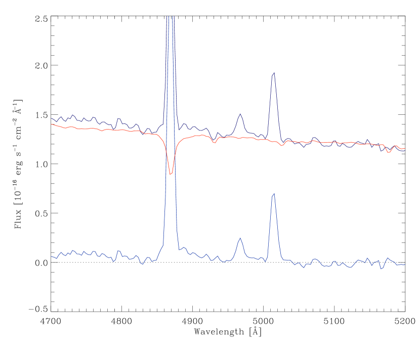
Figure 8: Example of a region with low emission in [O III] and a “deficient” SSP continuum subtraction (red line). Note that the SSP fit does not trace accurately the observed continuum (dark blue), leading to deviations from the theoretical [O III] $\lambda$5007/$\lambda$4959 ratio on the residual spectrum (light blue).

The “physically-selected” sample was qualitatively compared with the fibre-by-fibre sample. All the line ratios, spectral trends, level of dispersion and ionization properties described by the fibre-by-fibre sample were completely followed by the new limited sample, with only one important difference: the new sample discarded regions with low emission in oxygen, e.g. log([O III]/H$\beta$) below –1, points which are present in the case of the fibre-by-fibre sample, as shown in Fig. 6. Given that the selection criteria considered a lower flux threshold than in the fibre-by-fibre case, the flux limit cannot account for this effect. Therefore, the reason for the lack of these regions is due to the selection criterion based on the restricted range in the [O III] ratio.

Regions with low emission in oxygen correspond to the inner parts of the galaxy, where the stellar population is more dominant in the observed spectra, and therefore, the errors in the measurement of the residual emission lines due to a deficient continuum subtraction during the SSP model fitting are larger (e.g. see Fig. 8). For the outer regions of the galaxy, the contribution of the stellar population is lower, and therefore, it is easier to recover the proper [O III] ratio from the derived residual spectrum. However, in a region where the stellar population is more dominant and the emission lines are weak, the derived [O III] ratio from the residual spectrum might not be close to the theoretical ratio, but nevertheless, the total flux of these lines and their line ratios are representative of the physical conditions of the gas in that particular region. The fact that the inclusion of spectra with “non-physical” [O III] line ratios in the fibre-by-fibre sample produced well-defined trends (although with some level of scatter) in those weak oxygen (inner) regions give support to this idea.

In summary, the fibre-by-fibre method considered that each individual fibre samples a large-enough physical region of the galaxy and contains enough information for a complete spectroscopic analysis. Thanks to the different spectra selection steps, we were able to identify areas within the galaxy disk consistent with regions of nearly pure diffuse emission (in H$\alpha$ and H$\beta$), and to differentiate those from areas with the characteristic emission of well-defined H II regions. The methodology introduced for the fibre-by-fibre sample will be implemented to the second extraction method considered for the IFS study of NGC 628, by performing similar quality/sanity checks and comparing the radial trends in the line emission and diagnostic diagrams derived from the fibre-by-fibre sample.

3.2 Method II: HII region catalogue

Traditionally, spectroscopic studies of nearby galaxies have been performed by targeting a number of (bright) H II regions over the surface of a galaxy, placing long-slits and/or fibres of different apertures on top the selected regions, and integrating the flux over that aperture. The classical chemical abundance diagnostics based on the observation of strong emission lines ratios (e.g. $R_{23}$), were conceived as empirical methods describing the physical properties of these large, spatially-integrated, and individually defined H II regions. The calibration of these metallicity indicators were performed by using grids of photoionization models for a given range of metallicities and ionization parameters, and therefore, are not based on observational data alone. Given the large parameter space under investigation, these calibrations have generally assumed spherical or plane-parallel geometries without considering the effects of the distribution of gas, dust, and multiple, non-centrally located ionizing sources. These geometrical effects may affect the temperature and ionization structure of the regions.

It has been argued that the geometrical distribution of ionization sources may partially account for the large scatter in metallicities derived using model-calibrated empirical methods (Ercolano et al., 2007, hereafter EBS07). According to recent results based on 3D photoionization models with various spatial distributions of the ionizing sources, for intermediate to high metallicities, models with fully distributed configurations of stars display lower ionization parameters than their fully concentrated counterparts. The implications of this effect varies depending on the sensitivity of the metallicity indicator to the ionization parameter (EBS07).

Generally speaking, results derived from the use of the empirical metallicity indicators should be considered within a statistical framework, as the error due to intrinsic temperature fluctuations and chemical inhomogeneities on a single region may be very large, even when the temperature of the region can be directly determined (e.g. Peimbert, 1967; García-Rojas et al., 2006; Ercolano et al., 2007). The spectra extracted in the previous selection method were based on assuming that the spectra of individual fibres would contain enough information in order to derive the physical properties of the region sampled by the individual fibre aperture. However, as shown in Fig. 5, the selected fibres trace morphologically complex regions, which do not resemble the classical picture of well-defined spherical H II regions. Some of the most prominent emitting regions are embedded in giant H II complexes without an established geometrical centre, and most importantly, as discussed in Sec. 7 of Ros10, regions which would be considered as individual H II regions in classical terms, show fibre-to-fibre variations on their emission line intensities.

One question that we might rise at this point is, in the case of the fibre-by-fibre sample, whether we are observing real point-to-point variations of the physical properties within a region, i.e. if the different measured line ratios are reflecting a real distribution of the ionizing sources, gas content, dust extinction and ionization structure within these regions, or the line intensity variations are just spurious effects due to the relatively low signal-to-noise of those emitting regions. In that respect, one of the main issues that IFS observations of emission line regions should aim to assess is: how valid are the results derived from the use of strong line calibrators applied on a point-to-point (fibre-to-fibre) basis? compared to the co-added spectrum of a larger, classically well-defined H II region. In order to try to answer this question, and at the same time perform a robust 2D spectroscopic analysis of NGC 628, an analysis method was envisaged based on considering “classical” H II regions as the source of analysable spectra. For doing so, a number of H II regions in NGC 628 was identified and classified by hand, based on the H$\alpha$ emission line map of the galaxy and on the diffuse plus fibre-by-fibre spatial distribution of fibres, as shown in Fig. 5. The selection of the fibres considered to belong to an individual H II region was performed following a purely geometrical principle, i.e. fibres located within the same region, which seemed to be geometrically connected, were considered as a single H II region. This criterion might be relatively subjective, but “classical” H II regions in other spectroscopic studies were chosen following the same principle, e.g. by selecting the more prominent (high surface brightness) regions in H$\alpha$ narrow band images.

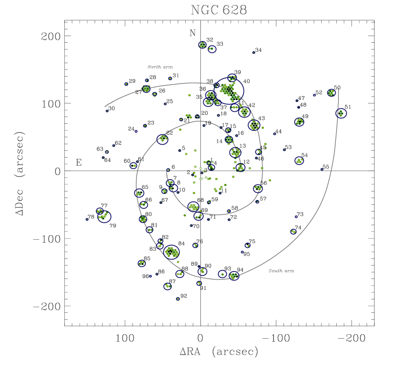
Figure 9: Spatial location and identification of the selected H II regions for NGC 628. The background fibres correspond to the fibre-by-fibre sample, with colour intensities scaled to the flux of the H$\alpha$ emission line. The circles correspond to the real or equivalent aperture diameter, as explained in the text. The grey-thick lines define the North and South operational spiral arms, as in Fig. 1 of Kennicutt & Hodge (1980).

The actual mechanism in order to generate the H II region catalogue for NGC 628 was the following:

1. A group of fibres is identified by eye as an individual H II region from the sub-mosaic extracted from the clean–residual mosaic, corresponding to the diffuse plus the fibre-by-fibre samples, as shown in Fig. 5. The positions and IDs of the selected fibres are stored and associated to the corresponding H II region. The fibre selection mechanism was based on two different methods: 1) by choosing the fibres individually by hand, following the morphological structure of the selected H II region; and 2) by considering all the fibres within a pre-established circular aperture centered at an arbitrary position, which might not coincide with the centre of any specific fibre. In the first case, the associated “location” of the H II region corresponds to centre of the first selected fibre, which was chosen to coincide nearly with the geometrical centre of the group of fibres considered as a H II region. In the second case, the location of the H II region corresponds to centre of the circular aperture, which was also chosen to coincide with the geometrical centre of the H II region. In the case of the circular aperture, different diameters were tested until the encompassed fibres would correspond to the visually selected region.

2. Once the positions and IDs of the fibres corresponding to a given H II region are identified in the sub-mosaic described above, the fibres corresponding to the same positions and IDs are recovered from the clean–observed mosaic, i.e. the RSS file before performing the SSP model subtraction. The spectra belonging to those fibres are co-added, obtaining a single spectrum corresponding to the selected H II region.

3. The integrated H II region spectrum is fitted by a linear combination of SSP templates by exactly the same procedure as described before, in order to decouple the contribution of the stellar population. Once the model of the underlying stellar population was derived, this is subtracted from the original spectrum, obtaining a residual H II region spectrum.

4. Individual emission line fluxes are measured from the residual spectrum by fitting single Gaussian functions as explained previously, obtaining a set of emission line intensities for each H II region.

5. The process is repeated for each group of fibres identified as a single H II region, until the whole surface of the galaxy mosaic is covered.

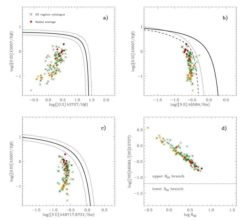
Figure 10: Diagnostic diagrams for NGC 628 corresponding to the selected H II regions catalogue (green symbols), the (reddish) diamonds correspond to the azimuthally-averaged radial values. Lighter tones correspond to inner regions of the galaxy, darker colours to increasing galactocentric distance. The different lines correspond to the theoretical boundaries dividing star-forming regions from other types of ionization. See the caption of the similar Fig. 6 for references and a more complete explanation.

A total of 108 H II regions were selected following the procedure described above. The residual spectra of the catalogue was tested against the quality criteria outlined in the case of the fibre-by-fibre analysis (i.e. the presence of [O II], [O III] and finite floating numbers for the derived value of c(H$\beta$)). Twelve spectra did not satisfy all the criteria and were discarded from the final catalogue. Fig. 9 shows the final sample of 96 selected H II regions for NGC 628. The fibres displayed in this figure correspond to the fibre-by-fibre sample shown in Fig. 5 (the diffuse sample was not included for the sake of clarity). The circles define the selected H II regions, the numbers next to the circles correspond to the H II region ID used in this paper. The diameter of the circles correspond to: 1) an “equivalent aperture” in the case where the H II region was selected by choosing individual fibres by hand, e.g. region N628–40, at ($\Delta\alpha$, $\Delta\delta$) $\sim$ (–40,130); 2) to the real diameter of the circular aperture when the selected H II region was chosen on this basis. Note that some fibres in Fig. 9 are not associated with any H II region (especially in the central region of the galaxy), these fibres correspond to the H II regions discarded due to the reasons explained in the previous paragraph. Note also that many H II regions are consistent with a single fibre. In those cases, the area surrounding the individual fibre did not show spectra with significant signal; therefore, they were not considered as their inclusion would only add noise to the integrated spectrum.

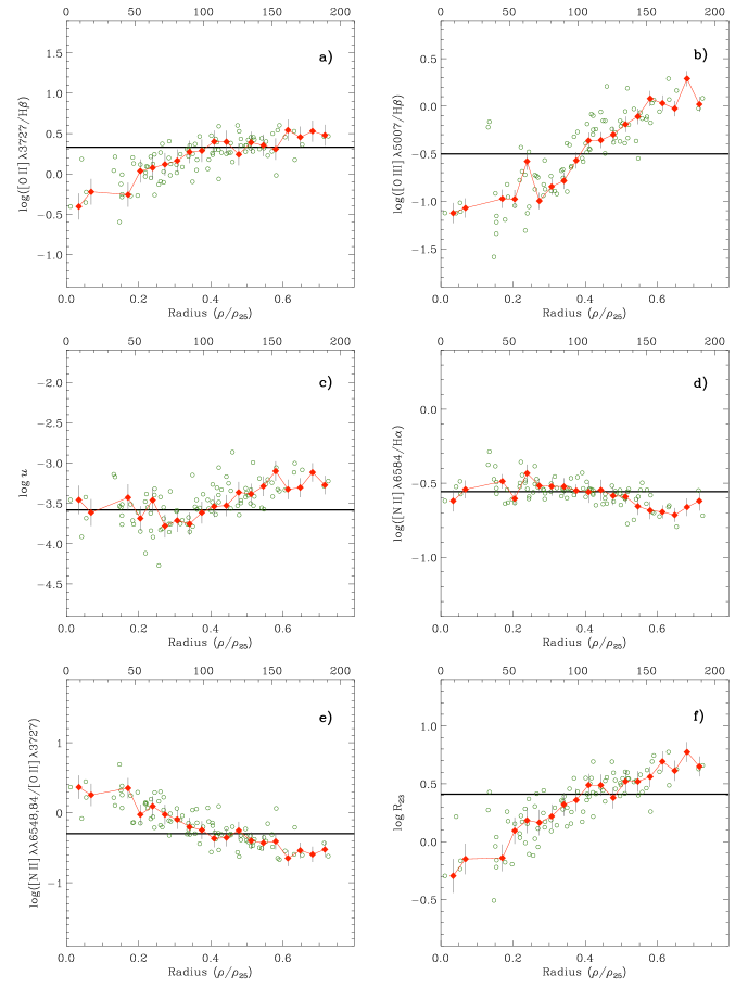
Figure 11: Radial variation of different line ratios and physical properties of NGC 628 for the H II regions catalogue (green circles) and the azimuthally-averaged spectra (red diamonds). Characteristic error bars are only drawn for the radial-averaged spectra for the sake of clarity. See the caption of the similar Fig. 7 for a full explanation.

After the quality of the derived spectra was confirmed by applying the same sanity-checks as in the fibre-by-fibre case, we proceeded to correct the measured emission line intensities by extinction in order to derive the physical properties from this new sample. Given the higher signal-to-noise of the H II regions compared with the previous samples, the logarithmic extinction coefficient c(H$\beta$) was obtained using both the H$\alpha$/H$\beta$ and H$\gamma$/H$\beta$ line ratios. The extinction law of Cardelli et al. (1989) with a total to selective extinction ratio $R_{V}=3.1$ was adopted for the interstellar reddening correction. Formal errors were derived by propagating in quadrature the uncertainty in the flux calibration, the statistical error of the line emission fluxes and the error in the c(H$\beta$) term. Additional information of the H II regions catalogue, including ID, coordinates, offsets, extraction method, equivalent/real aperture diameter (in arcsec and pc), and the number of extraction fibres for each selected H II region are included in Appendix B.

Fig. 10 and Fig. 11 show the diagnostic diagrams and radial trends derived from the H II region catalogue of NGC 628(green symbols), and a radial average spectra sample (reddish diamonds), obtained after co-adding successive annulus of 10 arcsec in an azimuthally radial way, as in the previous cases. Comparison of these plots with the corresponding diagrams of the fibre-by-fibre sample show that, in general terms, all trends are exactly reproduced, with the difference being the lower level of scatter in the case of the H II region catalogue diagrams. As in the previous similar plots, lighter colours in Fig. 10 correspond to inner regions in the galaxy, darker tones to outer parts. In particular, Panel a) of Fig. 10 shows a clear trend of increasing oxygen intensity for both [O II] and [O III] species as a function of radius. The trends shown in the rest of the panels show much narrower correlations than in the case of the fibre-by-fibre analysis, extending to relatively low ratios of [O II] $\lambda$5007/H$\beta$ and $\log R_{23}$, i.e. corresponding to the innermost regions of the galaxy. The [N II]/[O II] ratio obtained from the H II regions sample confirms that all the spectra are consistent with $R_{23}$ values corresponding to the upper branch of the O/H vs. $R_{23}$ relation.

The radial trends shown in Fig. 11 are consistent with those derived for the fibre-by-fibre sample, where spectra of the inner regions of the galaxy ($\rho\lesssim 0.3\rho_{25}$) were included by the selection criteria. In the case of the H II region catalogue, the number of regions sampling this zone is low, but they are enough to indicate the trends of all the line ratios and to produce reliable radial-averaged spectra. Furthermore, the scatter in the inner regions has been reduced compared to the similar fibre-by-fibre plots. For radii $\rho>0.4\rho_{25}$, the trends for all three different methods are practically identical, with a lower level of scatter for the H II regions sample. The position of the H II regions cover practically all radii from the inner regions of the galaxy (where the closest H II region to the centre is located at $\rho/\rho_{25}\sim$ 0.01), to the outer parts (where the H II region with the largest radius is $\rho/\rho_{25}\sim$ 0.72). However there is a gap between $\rho/\rho_{25}\sim$ 0.05 and 0.15 where no H II regions are found.

3.3 Comparison with H II regions from the literature

Table 2: H II regions within the IFS mosaic of NGC 628 observed by previous long-slit spectroscopic studies. Columns. (1-2): H II region identification in this work and the corresponding one found in the literature. (3-4): Offsets of the coincident H II regions in arcsec; in the case of PINGS, the offsets are reported with respect to the centre of the IFS mosaic ($\alpha$: 24.17410, $\delta$: 15.78392, 2000 equinox). (5): Galactocentric radius normalised to the size of the optical disc at the $B_{25}$ mag arcsec^-2 isophote. (6-7): Value of the $R_{23}$ index, defined as the ratio of the emission line intensities: ([O II] $\lambda$3727 + [O III] $\lambda$$\lambda$4959, 5007)/H$\beta$. (8): References. 1: Talent (1983); 2: McCall et al. (1985); 3: Bresolin et al. (1999); 4: Ferguson et al. (1998); 5: van Zee et al. (1998b).

	Region ID			Region offset ($\Delta\alpha$,$\Delta\delta$)						$R_{23}$
	PINGS	Literature		PINGS			Literature		$\rho/\rho_{25}$	PINGS	Literature	Reference
	(1)	(2)		(3)			(4)		(5)	(6)	(7)	(8)
1	N628–22	H292		50	46		49	52	0.23	1.67 (0.20)	2.59 (0.39)	1
											3.04 (0.34)	2
											2.44 (0.17)	3
2	N628–51	H154-155		-186	85		-186	86	0.72	4.24 (0.19)	4.84 (0.46)	2
											5.29 (0.24)	3
3	N628–56	FGW628A		-75	-26		-73	-29	0.26	1.30 (0.17)	2.28 (0.08)	4
		H451					-74	-22			1.81 (0.27)	1
											1.65 (0.18)	2
											1.75 (0.18)	3
4	N628–75	H572		-62	-110		-60	-107	0.39	2.28 (0.23)	2.97 (0.41)	2
											2.82 (0.18)	3
5	N628–84	H598		38	-120		42	-116	0.41	2.66 (0.21)	3.49 (0.52)	1
											3.55 (0.41)	2
											3.13 (0.25)	3
6	N628–85	+081-140		77	-137		81	-140	0.55	3.28 (0.15)	3.68 (0.08)	4
7	N628–87	+044-175		43	-171		44	-175	0.60	4.92 (0.18)	4.55 (0.11)	4
8	N628–94	H627		-44	-155		-42	-154	0.51	3.95 (0.19)	4.80 (0.52)	1
											5.02 (0.18)	2
											4.24 (0.18)	3
9	N628–96	+062-158		66	-156		62	-158	0.57	2.89 (0.18)	2.67 (0.16)	4

The PINGS IFS mosaic of NGC 628 covers a substantial fraction of the disc of the galaxy, therefore we are in the position to compare the emission line ratios and metallicity abundances derived in this work, with the coincident H II regions analysed by previous long-slit spectroscopic studies. A total of 47 independent observations of H II regions are reported in the literature for this galaxy, the first observations were performed by Talent (1983) (hereafter Tal83) who observed 5 H II regions from the catalogue of Hodge (1976), 7 correspond to McCall et al. (1985) (hereafter MRS85), 18 to van Zee et al. (1998b) (hereafter vZ98), 6 to Ferguson et al. (1998) (hereafter FGW98), 7 to Bresolin et al. (1999) (hereafter BKG99) and 4 to Castellanos et al. (2002) (hereafter CDT02); the spectroscopic analyses by Zaritsky et al. (1994) and Moustakas et al. (2010) made use of the line ratios provided by the previous references. The 5 H II regions observed by Ta83 were included in the sample observed by MRS85, the 7 regions observed by BKG99 are the same as MRS85 (with different wavelength coverage), region 628A from FGW98 is the same as region H451 from MRS85 and BKG99, and region H13 present in Tal83, MRS85 and BKG99 was also observed by CDT02. Therefore, the total number of non-duplicated H II regions found in the literature for NGC 628 is 33.

Only 9 of these regions fall within the FOV of the IFS mosaic observed by PINGS, they were identified with the corresponding H II regions defined in the previous section by comparing the offset reported in the literature and by visual inspection with Fig. 9. Table 2 lists the coincident H II regions observed by PINGS and previous long-slit spectroscopic studies, 6 of them have multiple observations, with N628–56 having the maximum number of references as it was observed by Tal83, MRS85, FGW98 and BKG99. Note that direct comparison between the H II regions reported in Table 2 has to be taken with caution, as the identification is somewhat ambiguous given the differences in the offsets between PINGS and the literature (due to the relatively arbitrary choice of the reference point in each study), but most importantly, to the different extraction apertures between long-slit observations and the fibre-defined H II regions of PINGS. Table 2 shows also the value of the $R_{23}$ index for each of the coincident regions compared with those reported in the literature. While in some cases we find a relative agreement (e.g. N628–51, 75, 85, 87, 96), the PINGS values are lower that the literature values in 7 of the 9 cases. However, even if we just consider the values found in the literature we find some important deviations in the reported $R_{23}$ index (e.g. N628–22, 51, 94). A thorough discussion of the comparison between the emission line ratios and the derived properties of these coincident H II regions will be presented in the next section.

3.4 On the spectra selection criteria

In this section we have explored two methods in order to extract spectra from an IFS mosaic in order to perform a 2D spectroscopic study. The first one considered the spectra contained in single fibres to be representative of the physical conditions of those regions sampled by the fibre aperture, while the second consisted in creating a catalogue of “classical” H II regions by co-adding fibres corresponding to the same morphological regions. The analysis of both samples resulted in similar trends but with a much reduced scatter in the case of the H II region spectra sample. From this exercise, we might be tempted to conclude that the best, or optimal selection method consists in obtaining a H II region catalogue in the “classical” sense, i.e. integrating the emission from a group of fibres associated to a given emitting region. However, we may leave open the possibility that –to some level– the scatter seen in the fibre-by-fibre sample might be actually due to intrinsic point-to-point variations of the emitting regions. It is important to note that this information is lost in typical long-slit spectroscopy, where the spectra is obtained very similarly as in the H II region catalogue method. The capability to detect these point-to-point variations, if real, might be one of the power of IFS observations. Some implications of the above findings are discussed in the following sections.

4 The IFS-derived abundance gradient of NGC 628

The gas-phase chemical content of NGC 628 has been previously analysed in a number of long-slit spectroscopic studies (e.g. Talent, 1983; McCall et al., 1985; Zaritsky et al., 1994; van Zee et al., 1998b; Ferguson et al., 1998; Bresolin et al., 1999; Castellanos et al., 2002; Moustakas et al., 2010). These works have derived the abundance gradient of NGC 628 up to relatively large galactocentric radii ($\rho\sim 1.7R_{25}$), using mainly empirical metallicity indicators based on the ratios of strong emission lines. They have found a higher metallicity content in the inner part of the galaxy, that the slope of the gradient is constant across the range of galactocentric distances sampled by the different studies, that the oxygen abundance decrease is relatively small, and that the average metallicity content is relatively high, consistent with solar and super-solar values. However, these results have been drawn from relatively few spectroscopically observed H II regions, and none of these within a radius of $0.2R_{25}$.

Apart of the previous spectroscopic studies mentioned in Section 4, Belley & Roy (1992) made use of imaging spectrophotometry, i.e. using narrow-band interference filters with the bandpass centered on several key nebular lines, in order to derive reddenings, H$\beta$ equivalent widths, diagnostic line ratios and metallicities for 130 H II regions across a large area of the galaxy disk. They found that the excitation, and some diagnostic line ratios are strongly correlated with galactocentric radius. They were able also to derive an oxygen abundance gradient of NGC 628, based on the [O III]/H$\beta$ ratio. Although strictly speaking, their results were not based on spectroscopic observations, this work represented an early and successful attempt to obtain the 2D distribution of the emission line properties of NGC 628.

The PINGS observations of NGC 628 allow to perform for the first time a full 2D spectroscopic abundance analysis based on the spectra samples obtained in the previous section, with an unprecedented number of spectroscopic data points. The reddening corrected line ratios for both the fibre-by-fibre and H II region catalogues were used to derived the oxygen abundance for each individual spectrum, using a subset of the abundance diagnostics employed in Paper I. Different abundance estimators were used in order explore the effects of a particular calibration depending on the physical properties of the galaxy , they correspond to a $R_{23}$-based calibrator (Kobulnicky & Kewley, 2004, hereafter KK04), an “index-empirical” method after Pettini & Pagel (2004) (hereafter PP04), and two additional strong-line empirical methods proposed by Pilyugin (2005) and Pilyugin (2007).

The KK04 calibrator is based on the stellar evolution and photoionization grids from Kewley & Dopita (2002), and takes into account the effects of the ionization parameter, providing parametrizations for both branches of the $R_{23}$ relation. A guess value of the metallicity has to be first inferred depending on the R₂₃ branch (previously determined from the [N II]/[O II] ratio, these nominal values (12+log(O/H)_lower = 8.2 and 12+log(O/H)_upper = 8.7) are used to calculate an ionization parameter $q$, i.e.

$$\log q = \{32.81-1.153y^{2}$$ (1)

$$+z(-3.396-0.025y+0.1444y^{2})\}$$

$$\times\{4.603-0.3119y-0.163y^{2}$$

$$+z(-0.48+0.0271y+0.02037y^{2})\}^{-1},$$

where $z\equiv{12+\log({\rm{O/H}})}$, $y\equiv\log O_{32}$ and

$$O_{32}={\frac{{\left[{{\rm{O\,III}}}\right]\lambda\lambda 4959,5007}}{{\left[{{\rm{O\,II}}}\right]\lambda 3727}}}.$$ (2)

The initial resulting ionization parameter is used to derive an initial metallicity estimate depending on the R₂₃ branch

$$12+\log({\rm{O/H}})_{{\rm{lower}}} = 9.40+4.65x-3.17x^{2}$$

$$-\log q({0.272+0.547x-0.513x^{2}}),$$

$$12+\log({\rm{O/H}})_{{\rm{upper}}} = 9.72-0.777x-0.951x^{2}$$

$$-0.072x^{3}-0.811x^{4}$$

$$-\log q(0.0737-0.0713x$$

$$-0.141x^{2}+0.0373x^{3}-0.058x^{4}),$$

where $x=\log R_{23}$. Equations 1 and 4 (or 4) are iterated until 12+log(O/H) converges.

The $O3N2$ index was first introduced by Alloin et al. (1979), a slightly different definition was proposed by PP04

$$O3N2=\log\left({\frac{{\left[{{\rm{O\,III}}}\right]\lambda 5007/{\rm{H}}\beta}}{{\left[{{\rm{N\,II}}}\right]\lambda 6584/{\rm{H}}\alpha}}}\right),$$ (5)

considering only the [O III] $\lambda$5007 line in the numerator. This ratio is sensitive to the metallicity as measured by the oxygen abundance through a combination of two effects. As O/H decreases below solar, there is a tendency for the ionization to increase (either from the hardness of the ionizing spectrum or from the ionization parameter, or both), decreasing the ratio [N II]/[N III]; on the other hand, the N/O ratio decreases at the high-abundance end, due to the secondary nature of nitrogen. The inclusion of [O III] could be useful in the high metallicity regime where [N II] saturates but the strength of [O III] continues to decrease with increasing metallicity. This index is almost independent of reddening correction or flux calibration. PP04 fitted the observed relationship between this ratio and $T_{e}$ based metallicities, obtaining monotonic relationship given by

$$12+\log({\rm{O/H}})=8.73-0.32\cdot O3N2,$$ (6)

valid for $O3N2<2$, with an estimated accuracy of $\sim$ $\pm$0.25 dex.

The third considered calibrator is the ff-$T_{e}$ method, i.e. the combination of the flux-flux (or $ff$–relation) proposed by Pilyugin (2005), and an updated version of the $T_{e}$-based method for metallicity determination (Izotov et al., 2006). The ff-relation links the flux of the auroral line [O III] $\lambda$4363 to the total flux in the strong nebular lines [O II] $\lambda$3727 and [O III] $\lambda$4959, $\lambda$5007. This relation is metallicity-dependent at low metallicities, but becomes independent at metallicities higher than 12+log(O/H) $\sim$ 8.25, i.e. the regime of high-metallicity H II regions. Using this relation, an inferred value of the [O III] $\lambda$4363 line can be derived, which translates to an electronic temperature of the high-ionisation zone $t_{3}\equiv$ $t$([O III]). Defining the following notations:

$$R=\frac{{\left[{{\rm{O\,III}}}\right]\lambda 4363}}{{{\rm{H}}\beta}},$$ (7)

$$R_{2}=\frac{{\left[{{\rm{O\,II}}}\right]\lambda 3727}}{{{\rm{H}}\beta}},\\$$ (8)

$$R_{3}=\frac{{\left[{{\rm{O\,III}}}\right]\lambda 4959+\left[{{\rm{O\,III}}}\right]\lambda 5007}}{{{\rm{H}}\beta}},$$ (9)

$$R_{23}=R_{2}+R_{3}.$$ (10)

we can express the excitation parameter $P$, as

$$P=\frac{{R_{3}}}{{R_{2}+R_{3}}}.$$ (11)

The $ff$ relation is defined as the relationship between the flux $R$ in the auroral line and the total flux $R_{23}$ in the strong nebular lines through a relation of the type $\log R=a+b\log R_{23}$, but since $R_{23}=R_{3}/P$, the $ff$ relation can be also expressed in the form $R=f(R_{3},P)$. This last relation was parametrised by Pilyugin et al. (2006) in the following way

$$\log R = -4.151-3.118\log P$$ (12)

$$+2.958\log R_{23}-0.680(\log P)^{2}.$$

From this equation, a ratio of the nebular [O III] $\lambda$4363 line to H$\beta$ is obtained, and therefore, a value of the electron temperature $T_{e}$ can be derived. This temperature, coupled with the observed strong-line intensity ratios are used in order to derive the chemical abundance using the revised direct method by (Izotov et al., 2006). The abundances derived through this method will be referred as the ff–$T_{e}$ abundances.

The last of the considered empirical calibrators is based on the prediction of the ratio Q${}_{\rm[N\,{\footnotesize II}]}$ = [N II] $\lambda$$\lambda$6548,6584/[N II] $\lambda$5755 from $R_{2}$ and $P$, using a calibration of high metallicity H II regions after Pilyugin (2007)

$$\log{\rm Q_{[N\,{\footnotesize II}]}} = 2.619-0.609\log R_{2}-0.010[\log R_{2}]^{2}$$

$$+1.085\log(1-P)+0.382[\log(1-P)]^{2}.$$

From this ratio, the value of the $t_{e}$([N II]) temperature is determined, which is taken as the characteristic temperature of the O⁺ low ionization region. Assuming $t_{e}$([N II]) $\approx$ $t_{e}$([O II]) $\approx$ $t_{e}$([S II]) $\equiv$ $t_{2}$, the $t_{2}$ temperature is determined via

$$t_{2}=\frac{1.111}{\log{\rm Q_{[N\,{\footnotesize II}]}}-0.892-0.144\log t_{2}+0.023t_{2}}.$$ (14)

The $t_{2}-t_{3}$ relation between the O⁺ and O⁺⁺ zones electron temperatures proposed by Pilyugin (2007) is used to derive the $t_{3}$([O III]) temperature, which is characteristic of the zone of high ionization:

$$t_{2}=0.41\frac{1}{t_{3}}-0.34P+0.81.$$ (15)

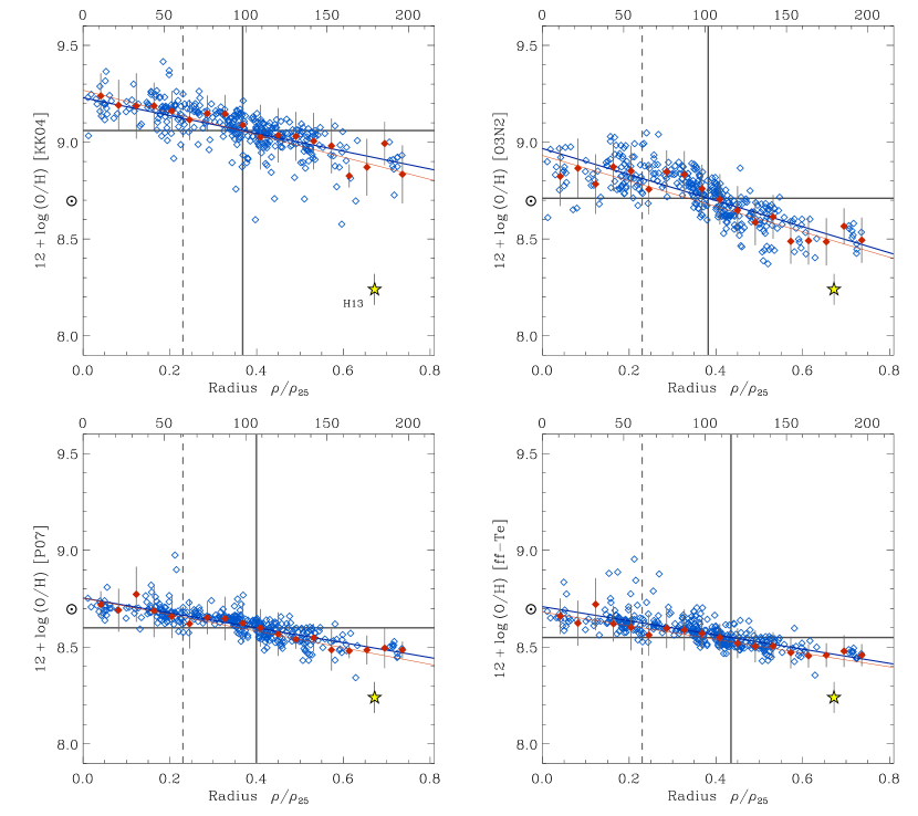
Figure 12: Radial abundance gradients derived for NGC 628 based on the fibre-by-fibre analysis (blue symbols) for different abundance diagnostics. The red diamonds correspond to the azimuthally-averaged radial spectra, for which characteristic error bars are drawn. The blue and red thick lines correspond to the linear least-squares fit to the fibre-by-fibre and radial average data points, respectively. The dashed vertical line marks the minimum radius of a H II region previously reported by the literature. The horizontal grey lines correspond to the abundance derived for a given calibrator using the integrated spectrum as reported in Paper I. The top $X$-axis values correspond to the projected radii in arcsec for the radial average data. The yellow star corresponds to the direct oxygen abundance of the H II region H13 derived by Castellanos et al. (2002).

This relation takes into account the effects of the excitation parameter $P$. Using these temperatures, the electronic density and the emission line intensities, the chemical abundances are derived using the equations of the direct method (Izotov et al., 2006). The abundances derived through this method will be referred as the P07 abundances.

One-dimensional radial abundance gradients for NGC 628 were derived based on the fibre-by-fibre and H II region catalogue samples for the different abundance diagnostics mentioned above. The radial gradients for the fibre-by-fibre sample are shown in Fig. 12. In each plot, the blue symbols correspond to the spectra of the fibre-by-fibre sample, the red diamonds correspond to the azimuthally-averaged radial spectra, as in previous figures. The radial average spectra show 1$\sigma$ error bars derived through a Monte Carlo simulation by propagating Gaussian distributions with a width equal to the errors of the emission line intensities, modulated by recomputing the distribution over 500 times. The errors of the fibre-by-fibre sample are slightly larger (due to the lower signal-to-noise of the individual spectra), but comparable in average with those calculated for the radial spectra (not drawn for the sake of clarity). The blue and red thick lines correspond to the linear least-squares fit to the fibre-by-fibre and radial average data points, respectively. In each panel, the values on the top $X$-axes correspond to the galactocentric distance in arcsec, the horizontal line correspond to the oxygen abundance value obtained from the integrated spectrum of the galaxy for that particular calibrator (see Paper I, ). The vertical solid line corresponds to the radius at which the fibre-by-fibre linear fit (blue line) equals the integrated abundance value. The solar abundance (12 + log(O/H)_⊙ = 8.70, Scott et al. 2009) is shown with the $\odot$ symbol in the $Y$-axes. The vertical dashed line marks the minimum galactocentric radius with reported observations of a H II region in the literature (H292 or FGW628A at 0.23$\rho_{25}$). Therefore, this work presents for the first time observations and chemical abundances of the innermost regions of NGC 628.

The yellow star in all panels of Fig. 12 corresponds to the oxygen abundance of the H II region H13 derived by CDT02, who were able to determine observationally the electronic temperature from optical forbidden auroral to nebular line ratios and to perform a direct oxygen abundance determination. This region represents the unique direct abundance measurement for NGC 628 reported in the literature, and it is included as an anchor abundance reference in order to compare the scales and offsets of the different abundance calibrators (the linear fits do not include this point in the calculation). No other points from the literature were considered when building the fibre-by-fibre abundance gradient, as the “source” of the spectra is conceptually different from those found in the literature (which are based on spectra integrated within apertures centered in classical H II regions); consequently, the baseline of the fibre-by-fibre abundance gradient spans just up to $\sim 0.75\rho_{25}$.

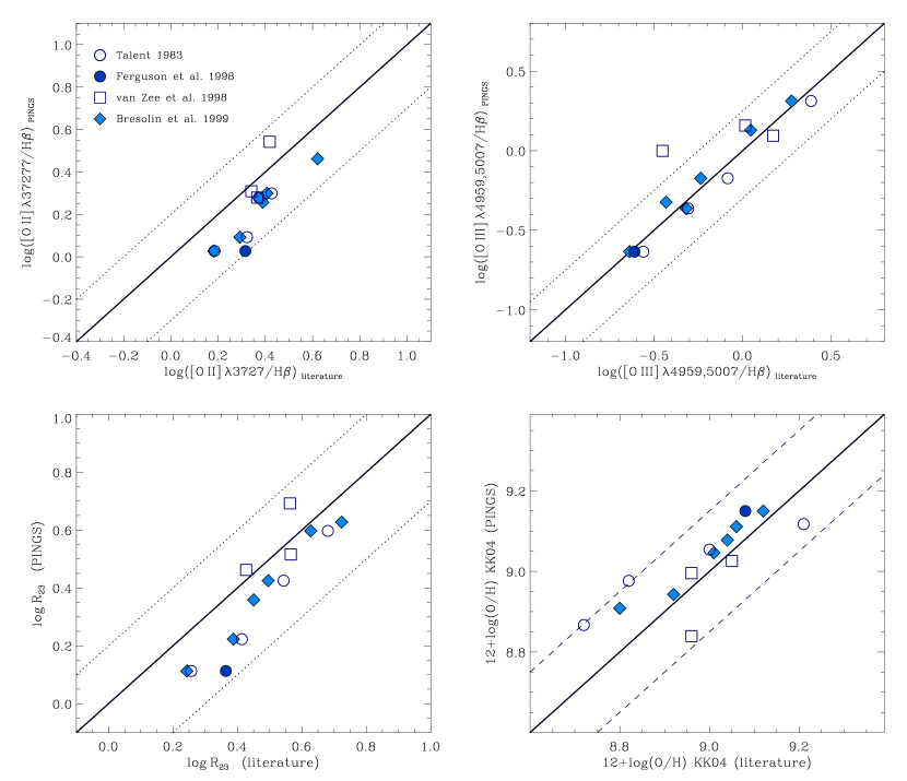
Figure 13: Comparison of the emission line intensities and oxygen abundance derived from this work with the coincident H II regions found in the literature within the FOV of the IFS mosaic of NGC 628. Top-left panel: [O II] $\lambda$3727/H$\beta$; top-right: [O III] $\lambda$$\lambda$4959,5007/H$\beta$; bottom-left: $R_{23}$ index; bottom-right: 12 + log(O/H) derived after the Kobulnicky & Kewley (2004) $R_{23}$-based calibrator. See the text for a full explanation.

The oxygen abundances derived using the $R_{23}$ KK04 method were calculated using the corresponding branch parametrization, based on the values of the [N II]/[O II] ratio as shown in Fig. 6. The $R_{23}$-based KK04 method shows a noticeable higher mean oxygen abundance, a higher level of dispersion for the same galactocentric radius, and a steeper slope than the rest of the other diagnostic methods. The gradient derived from the KK04 method is –0.46 $\pm$ 0.04 dex $\rho^{-1}_{25}$. The maximum oxygen values at $\rho=0$ inferred from this gradient is: 12 + log(O/H) = 9.23. The oxygen abundance derived from the integrated spectrum matches the linear fit for a radius $\rho/\rho_{25}$ very close to 0.4 ($\sim$ 100 arcsec). The scatter of the data points is somewhat larger than the intrinsic errors of the derived abundances, specially for regions located between 0.2 and 0.6 in normalised radius units. On the other hand, the radial average spectra shows a very linear relationship, with a low level of scatter. The gradient derived from the linear fit of this sample corresponds to –0.58 $\pm$ 0.06 dex $\rho^{-1}_{25}$, with corresponding central oxygen abundances of 9.27 in 12 + log(O/H) units.

The $O3N2$ derived gradient (top-right panel in Fig. 12) presents a similar trend to the $R_{23}$ KK04 calibrator, although it does not show a clear log-linear relationship as in the previous case. The pattern is more consistent with a semi-sinusoidal trend, with a steep gradient between 0.25 and 0.55$\rho_{25}$, a flattening of the gradient for the innermost and outermost regions of the galaxy (within the considered radial baseline), and a lower mean oxygen content with respect to KK04. The $O3N2$ abundances for those regions within 0.3$\rho_{25}$ show a large level of scatter, which is due to the combined effect of the high dispersion of the [N II]/H$\alpha$ and [O III]/H$\beta$ ratios observed for those zones (as shown in Fig. 7), but the scatter of the data is somewhat within the calculated error bars. The abundance gradients derived from the $O3N2$ calibrator are –0.67 $\pm$ 0.03 and –0.66 $\pm$ 0.07 for the fibre-by-fibre and radial average samples respectively, with central oxygen abundances of 8.97 and 8.93 in each case. Similarly to the $R_{23}$ method, the oxygen abundance obtained from the integrated spectrum matches the $O3N2$ linear fit at normalised radius $\sim$ 0.4.

The fibre-by-fibre oxygen abundance gradient based on the P07 and ff–$T_{e}$ method are shown in the bottom panels of Fig. 12. Both show very similar trends in terms of the mean abundance scale and steepness of the gradient. The scatter of the data points along all galactocentric radii is of the same level than the corresponding error bars. However, for regions of the galaxy at $\rho\sim 0.2\rho_{25}$, the dispersion increases considerably with a number of outlying data points approaching oxygen values of 12 + log(O/H) $\sim$ 9.0 especially for the ff–$T_{e}$ calibrator. Considering that the signal-to-noise of the [O II] and [O III] emission lines for these inner regions of the galaxy is relatively low, this behaviour suggests that this method is sensitive to the signal-to-noise of the strong oxygen lines used in the determination of the oxygen abundance. The abundance gradient derived from the fibre-by-fibre sample based on the P07 calibrator is –0.38 $\pm$ 0.02 dex $\rho^{-1}_{25}$ with a central abundance of 8.75, the same value as the radial average fit, but with a steeper gradient consistent with –0.43 $\pm$ 0.03 dex $\rho^{-1}_{25}$. In the case of the ff–$T_{e}$ method, the fibre-by-fibre gradient is –0.37 $\pm$ 0.02 dex $\rho^{-1}_{25}$, while the slope obtained from the radial average is –0.35 $\pm$ 0.03 dex $\rho^{-1}_{25}$, with central abundances of 8.71 and 8.68 respectively, i.e. the flatter gradients and lower central oxygen abundances among all the considered calibrators. As in the previous cases, the oxygen abundance determined from the integrated spectrum matches the ff–$T_{e}$ and P07 radial trends for a normalised radius $\sim$ 0.4. Table 3 summarises the results of the abundance gradients analysis of NGC 628 for the fibre-by-fibre sample. The first two columns for each of the metallicity indicators correspond to the fibre-by-fibre and radial average sample respectively. For each sample, the values of the extrapolated central abundance at galactocentric radius $\rho=0$, of the characteristic oxygen abundance at $\rho=0.4\rho_{25}$ (in 12 + log(O/H) units), and the slope of the abundance gradients in dex/$\rho_{25}$ and dex/kpc are presented.

Despite the evident scale offsets and small pattern variations among the different oxygen calibrators, all the metallicity gradients are quite similar in qualitative terms. They show a somewhat flat-distribution of the metallicity for the innermost region ($\rho<0.3\rho_{25}$) and a log-linear correlation between the oxygen abundance and galactocentric distance for the outer radii ($0.3<\rho/\rho_{25}<0.8$), the slopes derived from the fibre-by-fibre and radial average samples are equivalent within the errors, and as a common interesting feature, the integrated abundance for all the indicators coincides with the H II region abundance gradient for a normalised radius $\rho/\rho_{25}\sim 0.4$, i.e. that the integrated abundance correlates with the spatially resolved abundances, independent of the abundance calibration used. This effect was previously indicated by Moustakas & Kennicutt (2006), who observed –to a first order– that the abundance inferred from the integrated spectrum of a galaxy is representative of the gas-phase oxygen abundance at $\rho=0.4\rho_{25}$, i.e. the characteristic abundance of a galaxy, even in the presence of an abundance gradient, emission from the diffuse medium or variations in dust reddening. They reached this conclusion based on the ($R_{23}$ based) McGaugh (1991) calibrator (hereafter M91) and the Pilyugin & Thuan (2005) (empirical-index) calibrator. The latter showed a similar behaviour in their sample, but with a much higher dispersion. Here we confirm this result for the case of NGC 628, extending the number of calibrators also showing this trend.

Furthermore, the comparison between different calibrators helps us to infer some trends that are not noticeable when employing only one type of metallicity estimator. For example, the $O3N2$ and P07 methods somewhat suggest a flattening of the gradient for the innermost of the galaxy (for radii $<0.3\rho_{25}$), and a large dispersion in the log(O/H) values, with differences up to $\pm 0.5$ dex. Obviously, the central ($\rho=0$) and mean oxygen abundances are different considering the well-known offsets between the empirical calibrators, but even taking into account these discrepancies, it is interesting that the H13 H II region with the direct oxygen abundance measurement (12 + log(O/H) = 8.24 at 0.67$\rho_{25}$), lies significantly below the metallicity content inferred by any of the strong-line abundance calibrators at the same galactocentric distance, especially with respect to the KK04 calibrator, with an offset of $\sim$ 0.7 dex. If the oxygen abundance of the H13 H II region is considered reliable, these offsets indicate that the empirical calibrations overestimate the metallicity content of the NGC 628 H II regions by a factor between 2 ($O3N2$, P07, ff–$T_{e}$) and 5 (KK04), in accordance with recent studies comparing the abundances provided by the direct method with those obtained through empirical calibrations for star-forming regions (López-Sánchez & Esteban, 2010; López-Sánchez et al., 2011).

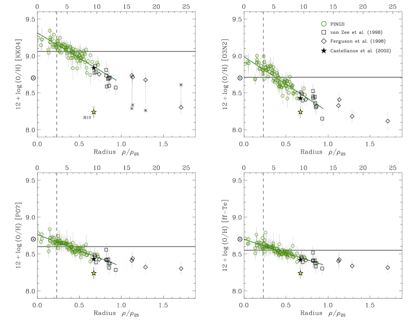
Figure 14: Radial abundance gradients derived for NGC 628 based on the PINGS H II region catalogue (green symbols), and H II regions from the literature (black symbols). For the KK04 estimator, we show two dotted-connected abundance values for those H II regions with an ambiguous choice on the $R_{23}$-branch. The yellow star corresponds to the $T_{e}$-derived abundance of the H II region H13 by Castellanos et al. (2002). Note the flattening of the gradient for radii $\gtrsim\rho_{25}$. See the text and the caption of the similar Fig. 12 for a full explanation.

The large number of spectroscopic points provided by this work has allowed us to build the most detailed metallicity gradient of NGC 628 within the optical radius of the galaxy. However, the radial baseline of the fibre-by-fibre sample is relatively short in order to account for the true behaviour of the abundance gradient of NGC 628. Nevertheless, we can made use of emission-line measurements of H II regions found in the literature (which span up to $1.7\rho_{25}$), in order to cover a larger galactocentric baseline of the galaxy. Oxygen abundances for the 47 reported H II regions found in the literature were calculated using published emission line ratios and by applying the four strong-line calibrators introduced previously. These values were incorporated to the oxygen abundances derived from the H II region catalogue sample observed by PINGS. Seventeen H II regions from the literature are located at $\rho\gtrsim 0.7\rho_{25}$, i.e. the maximum baseline of the PINGS H II region sample, permitting a much better characterisation of the radial abundance gradient.

Table 3: Radial abundance gradients for NGC 628. For each of the metallicity calibrators employed, the results from the fibre-by-fibre sample, radial average and H II region catalogue are presented. The rows correspond to: the central abundance at galactocentric radius $\rho=0$; the characteristic abundance at $\rho=0.4\rho_{25}$; and the slope of the abundance gradients in dex $\rho^{-1}_{25}$ and dex kpc^-1, respectively. Given the flattening of the abundance gradient for the outer parts of the galaxy, the values obtained from the linear fite were derived only for those regions with $\rho<\rho_{25}$, as explained in the text.

	KK04			O3N2
	Fibre-by-fibre	Radial	H II regions	Fibre-by-fibre	Radial	H II regions
12 + log(O/H)ρ=0	9.23 $\pm$ 0.02	9.27 $\pm$ 0.02	9.31 $\pm$ 0.02	8.97 $\pm$ 0.01	8.93 $\pm$ 0.03	8.99 $\pm$ 0.02
12 + log(O/H)${}_{\rho=0.4\rho_{25}}$	9.05 $\pm$ 0.02	9.04 $\pm$ 0.02	9.04 $\pm$ 0.02	8.70 $\pm$ 0.01	8.67 $\pm$ 0.03	8.69 $\pm$ 0.02
log(O/H)${}_{\rm(dex~{}\rho^{-1}_{25})}$	–0.46 $\pm$ 0.04	–0.58 $\pm$ 0.06	–0.68 $\pm$ 0.03	–0.67 $\pm$ 0.03	–0.66 $\pm$ 0.07	–0.75 $\pm$ 0.04
log(O/H)${}_{\rm(dex~{}kpc^{-1})}$	–0.033 $\pm$ 0.003	–0.041 $\pm$ 0.004	–0.048 $\pm$ 0.002	–0.048 $\pm$ 0.002	–0.047 $\pm$ 0.005	–0.053 $\pm$ 0.003

	P07			ff–$T_{e}$
	Fibre-by-fibre	Radial	H II regions	Fibre-by-fibre	Radial	H II regions
12 + log(O/H)ρ=0	8.75 $\pm$ 0.01	8.75 $\pm$ 0.01	8.76 $\pm$ 0.01	8.71 $\pm$ 0.01	8.68 $\pm$ 0.01	8.70 $\pm$ 0.01
12 + log(O/H)${}_{\rho=0.4\rho_{25}}$	8.60 $\pm$ 0.01	8.58 $\pm$ 0.01	8.59 $\pm$ 0.01	8.56 $\pm$ 0.01	8.54 $\pm$ 0.01	8.55 $\pm$ 0.01
log(O/H)${}_{\rm(dex~{}\rho^{-1}_{25})}$	–0.38 $\pm$ 0.02	–0.43 $\pm$ 0.03	–0.43 $\pm$ 0.02	–0.37 $\pm$ 0.02	–0.35 $\pm$ 0.03	–0.37 $\pm$ 0.02
log(O/H)${}_{\rm(dex~{}kpc^{-1})}$	–0.027 $\pm$ 0.001	–0.030 $\pm$ 0.002	–0.031 $\pm$ 0.002	–0.026 $\pm$ 0.001	–0.025 $\pm$ 0.002	–0.026 $\pm$ 0.001

The determination of the oxygen abundance for the H II regions found in the literature allow us to make a direct comparison of the metallicity content for the coincident H II regions within the FoV of PINGS, based on the values of the published (literature) and observed (PINGS) emission line intensities. Fig. 13 shows this comparison, the top-panels correspond to the comparison between [O II] $\lambda$3727/H$\beta$(left), and [O III] $\lambda$$\lambda$4959,5007/H$\beta$(right), while in the bottom we compare the $R_{23}$ index (left), and the 12 + log(O/H) derived after the Kobulnicky & Kewley (2004) $R_{23}$-based calibrator, i.e. the method in which we find the larger disagreement between PINGS and the literature abundance. For the 6 common regions between MRS85 and BKG99, only those by BKG99 are drawn (blue-filled diamonds). N628–56 is also common with FGW98, shown as a blue-filled circle. The regions common to vZ98 are drawn as open squares. In each panel, the solid line represents equality between the values, the dashed lines in the bottom-right (abundance) panel stand for a typical $\pm 0.2$ dex error associated with the determination of an oxygen abundance through the KK04 metallicity calibrator (and generally speaking, to any strong-line method). The dotted lines in the other panels stand for the error that the corresponding emission line ratio (or index) should posses in order to account for the $\pm 0.2$ dex error of the abundance determination, i.e. if we propagate back the uncertainty in the metallicity determination as due to a difference in a particular emission line ratio or index. Note that these errors are not symmetric due to the definition of the KK04 calibrator (based on the $R_{23}$ index), as defined in Eq. 1 to Section 4.

The values of the emission line ratios and the derived oxygen abundance show in general a good agreement between both samples. Note that any difference between the observed (PINGS) and published (literature) data fall within the errors, as defined by the $\pm 0.2$ dex intrinsic uncertainty of the KK04 strong-line calibrator, with the the exception of one H II region from vZ98 in the [O III]/H$\beta$ ratio. Any small deviation between the published and observed values is somewhat expected, considering that: i) the spatial identification of the H II regions is ambiguous; ii) the extraction apertures differ importantly between the previous long-slit and the fibre-based PINGS observations; iii) the emission line intensities found in the literature were obtained directly from the observed spectra, while in the case of this work, we measured the line intensities from the residual spectra which took into account the effects of the underlying stellar population; and iv) the reddening correction was performed with different extinction laws. Considering all these facts, the good agreement between the literature and PINGS values give us confidence regarding the high-quality of the spectra, and in general to the abundance analysis method for the IFS mosaic of NGC 628.

The derived abundance gradients for the PINGS H II region catalogue, plus the H II regions from the literature of NGC 628 are shown in Fig. 14, using the same abundance estimators as in the fibre-by-fibre case. In each panel, the green open-circles correspond to the PINGS H II region sample, while the black symbols correspond to H II regions from the literature. One-sigma error bars are display for each data point. For the sake of clarity, only those regions from the literature with $\rho\gtrsim 0.7\rho_{25}$ are drawn, since those with lower radii fall within the cloud of the PINGS data points, following the same trend marked by the inner H II regions. The $T_{e}$-derived oxygen abundance of the H13 H II region from Castellanos et al. (2002) is shown as a yellow star. The values on the top-horizontal axis correspond to the deprojected galactocentric distance in kpc. The dashed vertical line marks the minimum galactocentric distance of a H II region found in the literature ($\rho\approx 0.2\rho_{25}\approx 3$ kpc). At first glance, there is one noticeable feature in all four panels of Fig. 14, i.e. that the negative slope of the metallicity with increasing galactocentric radius changes to a nearly constant abundance for regions with $\rho\gtrsim\rho_{25}$, implying that there is flattening of the abundance gradient of NGC 628 for the outermost regions of the galaxy, feature that has not been previously reported for this galaxy.

All previous determinations of the abundances gradient for NGC 628 considered only regions within $\rho\lesssim\rho_{25}$, (e.g. Tal83, Zaritsky et al. (1994), vZ98, Moustakas et al. (2010)), with the exception of FGW98, who obtained an abundance gradient extending to $\rho\sim 1.8\rho_{25}$ based on 6 H II regions observed by these authors (two of them within the radii of the PINGS mosaic), and by adding 7 H II regions analysed previously by McCall et al. (1985) (all of them within the range of observed H II regions of this work), for a total of 13 regions. They made use of the $R_{23}$-based M91 calibrator, deriving a steep gradient 12 + log(O/H) = 9.08 $-(0.73\,\pm\,0.12)\rho/\rho_{25}$. The flattening of the oxygen abundance is somewhat apparent in their work (see Fig. 10 and 11 of vZ98). However, the lack of spectroscopic points between the inner and outer regions of NGC 628, and the choice of the $R_{23}$ branch in the calibration for the outer H II regions, made FGW98 infer that the abundance gradient of the galaxy was steep along all galactocentric radii.

The top-left panel of Fig. 14 shows the abundance gradient of NGC 628 derived after the KK04 $R_{23}$-based calibrator. For regions within $\rho_{25}$, the galaxy presents a clear steep negative gradient. However, for regions beyond that radius, the $R_{23}$ calibrator enters into the ill-defined region between the two $R_{23}$ branches. For each of the outer H II regions, the asterisk mark the value of the oxygen abundance derived from the opposite branch as defined by KK04, a dotted line connects the values of both branches. For those regions between $1\rho/\rho_{25}1.5$, FGW98 took the lower-branch O/H value, while according to the prescriptions of KK04 based on the [N II]/[O II] ratio, we determine the upper-branch values. From this example, it is evident that, when the metallicity is derived through a $R_{23}$-based calibrator, the choice of the $R_{23}$ branch plays an important role in defining the nature of the abundance gradient at larger radii, as it could lead to different interpretations, e.g. that the slope of the gradient is constant across all the galaxy, that there is a flattening of the oxygen distribution after a certain radius, or even that there is a break of the metallicity content of $\sim 0.3$ dex with respect to the edge of the optical disk.

In the top-right panel of Fig. 14 we use the $O3N2$ empirical-index calibrator (PP04) to construct the abundance gradient of NGC 628. Apart from the well-known shift in the metallicity scale with respect to KK04, we note in the outer zones a feature that can be either a flattening of the gradient to a constant metallicity, or a change in the slope to a nearly flat gradient. This feature is also present in the other two calibrators employed, P07 and ff$-T_{e}$, shown in the bottom panels of Fig. 14. These three –conceptually different– metallicity estimators suggest that this effect is indeed real, that the oxygen abundance decreases with increasing radius up to a point in which the variation in metallicity is almost negligible, and that there is no discontinuity in the radial abundance distribution, as one choice of the $R_{23}$ branch for the KK04 calibrator might incorrectly suggest.

Recently, (Bresolin et al., 2009) observed a flat oxygen abundance gradient and a drop in abundance beyond the $\rho_{25}$ isophotal radius of M83. The result was confirmed by a wide range of abundance indicators and tests considering the impact of different ionizations at larger radii. Likewise, Goddard et al. (2010) produced an accurate abundance gradient of the XUV spiral galaxy NGC 4625 out to $2.5\rho_{25}$, finding a flattering of the radial gradient in the outer disc and an apparent discontinuity in the abundance close to the optical edge of the disc. A possible interpretation of this feature may be an intrinsic difference in the star formation rate between the inner and outer disc linked to the 2D gas surface density. In this scenario, the formation of massive stars in the outer regions is rare, and therefore there is a lack of enrichment from supernovae in the outer disc compared with the inner regions. The results from this work give support to the existence of these features in nearby spiral galaxies, although the definite existence (and interpretation) of these attributes will require further observations and a larger statistical sample.

In all panels of Fig. 14, the green thick line corresponds to a linear least-squares fit applied to those regions within $\rho/\rho_{25}<1$. Table 3 shows the values derived from the abundance gradient fitting of the fibre-by-fibre, radial average and H II regions samples. Direct comparison among the different samples shows in general a good agreement in terms of the derived slopes and central abundances for each calibrator, with the exception of KK04, for which the central oxygen abundance is higher ($\sim 0.8$ dex) and the slope is much steeper ($\sim 0.2$ dex $\rho_{25}^{-1}$) for the H II region sample. The central oxygen values at $\rho=0$ are in agreement within 0.1 dex with the values obtained previously for the fibre-by-fibre sample. Likewise, the oxygen abundance derived from the integrated spectrum (horizontal gray-line) matches the H II region abundance of each calibrator for a radius $\rho\sim 0.4\rho_{25}$ for all methods. The slope of the gradient varies also considerably among different calibrators, with $O3N2$ showing the steepest value ($-0.75\pm 0.04$ dex $\rho_{25}^{-1}$), compared to the flatter slope of the ff$-Te$ method ($-0.37\pm 0.02$ dex $\rho_{25}^{-1}$), i.e. a difference of $\sim 0.38$ dex. The reason of this behavior might reside in the fact that, the metallicity determination with empirical indices based on the [N II] emission lines (e.g. $N2$, $O3N2$), overestimate the abundance at high N/O ratios and vice versa (Pérez-Montero & Contini, 2009), causing a larger difference in metallicity between the inner and outer H II regions of the galaxy.

Another interesting feature present in all panels of Fig. 14, is the high level of scatter in the oxygen abundance for a given radius within the innermost regions of NGC 628. In all cases, differences of $\sim 0.3$ dex in log(O/H) can be found for a given $\rho$. Furthermore, in all instances, the H II region with the maximum oxygen abundance is not located at $\rho/\rho_{25}\sim 0$, but at a distance of $\rho/\rho_{25}\sim 0.15$ ($\sim$ 2 kpc in physical scale), radius at which the higher dispersion in the oxygen abundance is found. As discussed in Paper I, previous IFS observations of the stellar component in the central core of NGC 628 showed a ring-like structure and an inversion of the metallicity gradient at $\sim$ 2 kpc (Wakker & Adler, 1995; Ganda et al., 2007), somewhat suggesting a dynamical cold inner disc. Based on the results of this work, the metallicity of the gas seems to follow the trend mark by the stellar populations at the centre of the galaxy. This result, together with the confirmed presence of circumnuclear star-forming regions in NGC 628, might indicate a scenario in which the gas is being radially transferred, inhibiting the enhancement of the gas-phase metallicity at the innermost regions of the galaxy, where a moderate drop or flattening of the abundance gradient can also be seen. The combination of the inner and outer structure of the metallicity distribution of NGC 628 suggests a multi-modality of the abundance gradient of the galaxy, consistent with a nearly flat-distribution in the innermost regions of the galaxy ($\rho/\rho_{25}<0.2$), a steep negative gradient for $0.2\lesssim\rho/\rho_{25}<1$, and a shallow or nearly-constant gradient beyond the optical edge of the galaxy.

4.1 The distribution of the N/O ratio

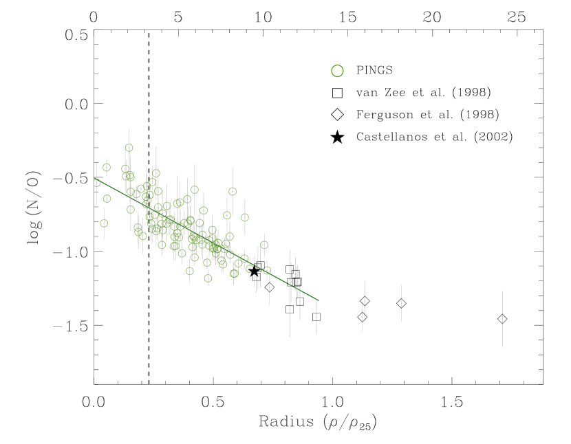
Figure 15: Radial distribution of the N/O ratio for the H II region catalogue of NGC 628, based on the results from the P07 calibrator. Green symbols correspond to the PINGS data, while black symbols stand for the H II regions drawn from the literature. The linear fit, shown as a thick green line, was only performed to those regions with $\rho<\rho_{25}$.

The nitrogen-to-oxygen radial distribution is shown in Fig. 15 with similar symbol-colour coding that the previous figure. The N/O ratio was calculated following the prescription by Hägele et al. (2008):

$$\log({\rm N^{+}/O^{+}}) = \log\frac{\rm[N~{}II]\,\,\,I(6548+6584)}{\rm[O~{}II]\,\,\,I(3727)}+0.281$$

$$-\frac{0.689}{t_{e}}+0.089\log t_{e}$$

assuming N/O = N⁺/O⁺ and $t_{e}\equiv t({\rm[N\,{\footnotesize II}]})=t({\rm[O\,{\footnotesize II}]})$, using the electronic temperature derived from the P07 calibrator.

The dispersion at a given radius is larger compared to the oxygen abundance gradient, the reason might reside in local effects related to the time delays between the release of primary and secondary nitrogen at different spatial regions of the galaxy but with coincident galactocentric radii (Costas & Edmunds, 1993). The distribution of the N/O ratio in the inner ($\rho<\rho_{25}$) part of NGC 628 decreases linearly with galactocentric radius, with a derived slope of the N/O gradient ($-0.88$ dex $\rho_{25}^{-1}$) being two-times steeper than that of the corresponding O/H gradient ($-0.43$ dex $\rho_{25}^{-1}$), as shown in Table 4 for both the fibre-by-fibre and H II region catalogue samples. The steeper N/O ratio is also present when considering the O/H gradient based on the ff–$T_{e}$ abundance estimator, with differences within 0.05 dex $\rho_{25}^{-1}$. These is in agreement with a previous determination of the N/O gradient for NGC 628, obtained by van Zee et al. (1998a) for 25 H II regions within $\rho_{25}$. They derived a gradient $-0.57$ dex $\rho_{25}^{-1}$ for the N/O ratio and $-0.99$ dex $\rho_{25}^{-1}$) for the O/H abundance, using the $R_{23}$-based M91 calibrator. Nevertheless, as in the case of the oxygen abundance gradient, the N/O ratio as a function of radius shows a clear flattening (and a lower level of dispersion) for regions $\rho>\rho_{25}$. This feature was also noted by FGW98, who inferred that the outer H II regions are consistent with a combination of primary and secondary production of nitrogen. Previous observations of the outermost H II regions in spiral galaxies have also found similar patterns and constant N/O ratios to those found in low metallicity H II regions in dwarf galaxies, where the production of nitrogen is mainly due to massive stars (e.g. Garnett, 1990; Thuan et al., 1995).

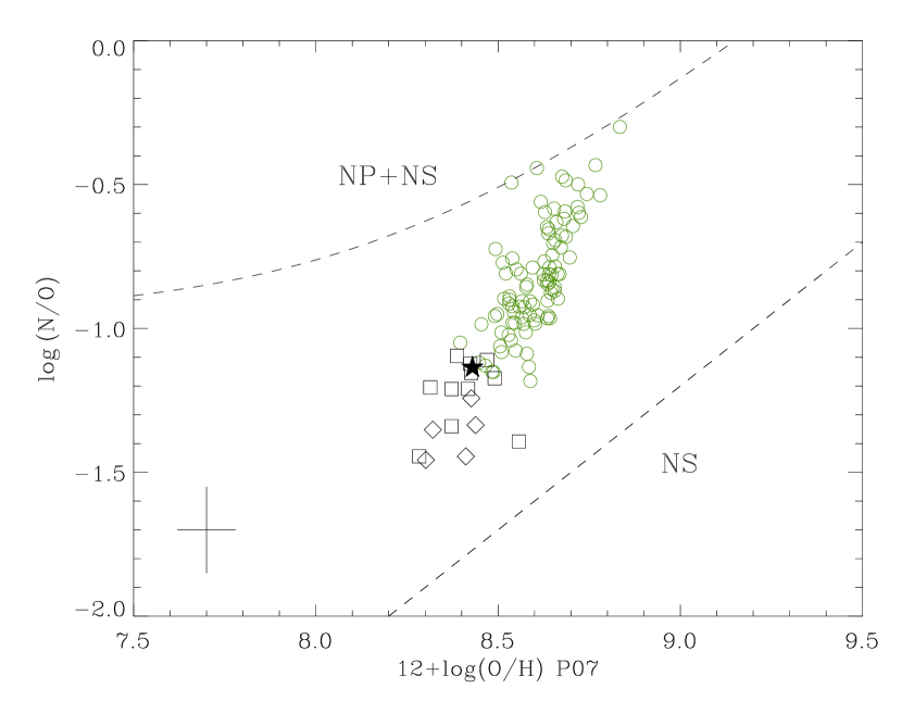
Figure 16: Observed N/O ratio as a function of the oxygen abundance 12 + log(O/H) as calculated using the P07 calibrator. Colour-symbol coding as in Fig. 15. The dashed lines show the relative abundance when N is secondary (NS), or a combination of primary and secondary (NP+NS).

Table 4: Radial gradient of the N/O ratio for NGC 628, based on the results from the P07 calibrator for both the fibre-by-fibre and H II region catalogue samples. The rows correspond to: the central value at galactocentric radius $\rho=0$; the characteristic ratio at $\rho=0.4\rho_{25}$; and the slope of the gradient in dex $\rho^{-1}_{25}$ and dex kpc^-1, respectively. The linear fit was only performed with those regions with $\rho<\rho_{25}$.

	P07
	Fibre-by-fibre	H II regions
log(N/O)ρ=0	-0.59 $\pm$ 0.06	-0.50 $\pm$ 0.03
log(N/O)${}_{\rho=0.4\rho_{25}}$	-0.92 $\pm$ 0.06	-0.86 $\pm$ 0.03
log(N/O)${}_{\rm(dex~{}\rho^{-1}_{25})}$	-0.83 $\pm$ 0.13	-0.88 $\pm$ 0.06
log(N/O)${}_{\rm(dex~{}kpc^{-1})}$	-0.059 $\pm$ 0.010	-0.062 $\pm$ 0.004

Further comparisons between the radial gradients of oxygen and nitrogen can provide us with clues regarding the chemical evolution of the galaxy. If nitrogen is a secondary element, the N/O ratio is expected to vary linearly with O/H with a slope $\geqslant 1$. In that case, the N/O gradient should be somewhat steeper than that shown by O/H (Henry et al., 2000). On the other hand, if the production of primary nitrogen is important, then galaxies tend to have shallower O/H gradients (van Zee et al., 1998a). As shown in Fig. 16, in the case of NGC 628 the N/O ratio increases linearly with oxygen abundance, as expected in the high metallicity regime of NGC 628, indicating that nitrogen is predominantly of secondary nature (Mollá et al., 2006). However, the innermost regions of the galaxy (with larger O/H) present N/O ratios which are larger than those expected by the pure secondary nature of nitrogen, resembling the N/O behaviour of some circumnuclear star-forming regions (CNSFR Díaz et al., 2007). This might be a signature of time delay between the release of oxygen and nitrogen, deviations from closed-box chemical evolution models, or even the presence of dynamical processes such as gas infall or outflow. In fact, as previously indicated by Mollá et al. (2006) using theoretical evolutionary models, the star formation efficiency plays a relevant role in the evolution of the relative abundance N/O, i.e. that differences in the star formation history of a particular galaxy (and/or regions within them), can explain the dispersion of the data of the N/O vs. O/H (and therefore vs. $\rho$) plane. Further improvements in the methods to calculate abundances and in the theory of galaxy chemical evolution are needed to better understand these trends.

4.2 Reliability of the O/H abundance gradient

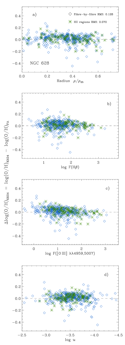
Figure 17: Scatter of the KK04 metallicity as measured by the $\Delta$log(O/H)_KK04 value, calculated with respect to the linear fit of the fibre-by-fibre sample (blue symbols) and the H II region catalogue (green symbols). Panel a): as a function of galactocentric radius; Panel b): as a function of the observed flux in H$\beta$; Panel c): as a function of the observed flux in [O III] $\lambda$$\lambda$4959,5007; Panel d): as a function of the ionization parameter $\log u$.

The linear fits for the inner region ($\rho<\rho_{25}$) of NGC 628 shown in Fig. 14 are based on a relatively large number of H II regions, considering that typical spectroscopic studies are performed with a handful of H II regions from which previous abundance gradients have been derive. As stated by many studies (e.g. Diaz, 1989), most of the H II regions observed in external galaxies fall under the category of Giant Extragalactic H II regions (GEHR). These correspond to very large H II regions with dimensions up to 1 kpc, and with a substantial number of ionizing stars. Being such extended regions, the nebulae would include zones of different physical conditions, gas in different degrees of ionization and different amounts of reddening. Therefore, the observations of these regions would lead to systematic errors of the total derived abundance, if the latter is inferred from calibrators based on photoionization models which fail to provide adequate ionization correction factors, ICF (i.e. the ratios between the total abundances of the various elements and the abundance in a single state of ionization), and/or if they do not consider the 3D geometrical distribution of the ionizing sources. As suggested by EBS07, if compact clusters (small H II regions) and loose associations (GEHRs or H II complexes) are randomly distributed throughout a given galaxy, the systematics errors on the observed metallicities at a given radius due to the effects mentioned above would only cause a larger scatter at a given galactocentric distance, and given a sufficient number statistics they would not affect the overall metallicity distribution. On the other hand, if the location of compact clusters and large associations are somewhat dependent on the galactocentric radius, then the systematic errors may introduce a bias on the measured metallicity gradient if the abundances are obtained from methods that do not take into account the differences on the excitation between small and large H II regions.

One way of assessing this issue is by comparing the results from metallicity indicators based on photoionization models (e.g. KK04), and those based on purely empirical methods. As discussed above, the most evident differences between the abundance estimators consists in the absolute metallicity scale and difference in the steepness of the gradient. However, considering that we benefit from a nearly complete spectroscopic coverage of small and large H II regions over the area of the galaxy where a gradient is present, give us the possibility to explore the systematics between different ways of obtaining the abundance gradients. One possibility is to select different sets of spectra in order to explore variations and systematics of the derived abundance gradients. This has been partially done, by considering the different spectra samples analysed so far. Nevertheless, the H II region catalogue offer us the possibility to discriminate between H II regions of different brightness and sizes, and therefore we can simulate for example, the abundance gradient determination based only on a few bright H II regions of a galaxy, like performed in most “classical” studies, and compare the results with the abundance gradients obtained from the full distribution of H II regions.

In order to perform this exercise, we chose 15 large (characteristic aperture $>$ 8 arcsec) and bright (log(L(H$\alpha$)) $>39$) H II regions from the PINGS catalogue of NGC 628, distributed over a good range of galactocentric distances, and selected from the four quadrants of the galaxy as defined in Fig. 9. The minimum galactocentric distance of these sample is $\rho/\rho_{25}\sim 0.18$, and the maximum is $\rho/\rho_{25}\sim 0.9$. As the derived gradients using these regions may be biased by their somewhat arbitrary selection, a statistical approach was followed in order to derive the abundance gradients from a bright H II region subsample. Eight regions were extracted randomly from the sample of 15 large/bright regions; the abundance gradients were then calculated from this H II region subsample. The process was repeated over 50 times for each abundance calibrator. Then we obtained a gradient, central oxygen and characteristic abundance from the mean values of the 50 realizations. The derived gradients resulted in very similar trends for all the considered calibrators, with variations in the central and characteristic oxygen abundances of the order of $\pm$ 0.05 dex. In terms of the derived slope, we find relatively low differences of the order of $\pm$ 0.1 dex $\rho_{25}^{-1}$, but consistent in average with steeper slopes and higher central oxygen abundances, compared to the abundance gradients obtained from the full catalogue of H II regions. The reason for this variation resides mainly in the spatial sampling of the bright H II regions, as in the innermost part of the galaxy there are practically no H II regions which fall under that category, and therefore, the H II regions at $\rho/\rho_{25}\sim 0.2$, which happen to posses a higher O/H abundance than the inner H II regions, have a higher weight in the linear fitting of the bright subsample, causing a higher central oxygen abundance and the steeper slope. However, in the case of NGC 628 these differences are negligible, considering the intrinsic systematic errors of the strong-line abundance determinations. Therefore, it seems that –to a first-order– the spatial distribution of compact clusters and large association of the galaxy do not affect significantly the measured metallicity gradients.

Another feature that might influence the determination of the metallicity gradient with a large number of spectroscopic points is the scatter in the metallicity for a given radius. By examining Fig. 12 and Fig. 14, we note that different abundance estimators present a different dispersion in the O/H values for a given $\rho$, with the KK04 $R_{23}$-based calibrator presenting (statistically) the higher level of scatter. One relevant question in the 2D IFS study of NGC 628 is whether this dispersion in metallicity is real or is just an artifact, maybe produced by the failure of a given metallicity calibrator in estimating the true abundance, due either to spectra of low S/N or spectra that do not correspond to the physical conditions for which the strong-line calibrator was modelled or calibrated.

Figure 18: Left: Histogram of the number of ionizing Lyman continuum photons Q(H⁰), as derived from the H$\alpha$ luminosity of the individual spectra in the fibre-by-fibre sample (blue) and H II region catalogue (green). The thick vertical line corresponds to the log Q(H⁰) value for an ionizing cluster of 10⁴ M_⊙ which is free of stochastic effects. Right: Histogram of the ionization parameter $\log u$ for both spectroscopic samples.

A possible explanation of the high level of scatter found in the fibre-by-fibre analysis may be statistical variations due to spectra that, despite the quality selection criteria, are of relatively low signal-to-noise compared with the integrated spectra of the H II regions catalogue. In this scenario, the line intensity variations would be just reflecting spurious effects due to the relatively weakness of those emitting regions. Panel a) of Fig. 17 shows the value $\Delta$log(O/H)_KK04 for each spectrum of the fibre-by-fibre sample (blue symbols) and the H II region catalogue sample (green symbols), calculated with respect to the log(O/H) value derived from the corresponding linear fit (at the same $\rho$ than the observed spectrum), i.e. the scatter of the log(O/H)_KK04 value as a function of radius. From this figure we can note that the level of scatter is higher for the fibre-by-fibre sample ($rms=0.128$) than for the H II region catalogue ($rms=0.070$), but that in general terms (with the exception of a few outliers), the dispersion in metallicity does not vary as a function of radius, i.e. there is not a preferential spatial position at which the scatter in the oxygen abundance is larger. The reason of the higher scatter for the fibre-by-fibre sample is most probably due to the smaller spatial sampling of the individual fibres compared to the integrated spectra of the H II regions, where the differences in the line emission has been averaged. Panels b) and c) of Fig. 17 show the $\Delta$log(O/H)_KK04 value as a function of the observed flux in H$\beta$ and [O III] $\lambda$4959 + $\lambda$5007 respectively. If the scatter in the metallicity was due to the low S/N of the observed spectra, then we would expect a “butterfly” pattern (e.g. see Fig. 2), consistent with higher dispersion in $\Delta$log(O/H)_KK04 for lower line strengths (where a lower S/N is expected), and vice versa. However, we do not see that pattern in panels b) and c) of Fig. 17, the level of scatter is relatively similar over more than two orders of magnitude in each case, and where the largest $\Delta$log(O/H)_KK04 values correspond to relatively high line intensities (especially in the [O III] lines).

On the other hand, if the observed dispersion in metallicity was due to the physical conditions of the emitting region (e.g. gas in different degrees of ionization), then we could expect that regions with different levels of excitation are more prone to deviations in the calculated oxygen abundance. Panel d) of Fig. 17 shows the $\Delta$log(O/H)_KK04 value as a function of the ionization parameter $\log u$. Again, we note that the scatter in metallicity does not seem to depend on a certain ionization parameter, and that the level of dispersion is similar for both spectroscopic samples over two orders of magnitude in $\log u$. All the above results suggest that, if the scatter in metallicity does not depend on any particular region of the galaxy, that is not due to the possible low S/N of the observed spectra, and that shows no systematic dependence with the ionization conditions of the gas, then the dispersion in metallicity for a given galactocentric radius is real, and it is reflecting a true spatial physical variation of the oxygen content.

Another question that might be raised regarding the reliability of the metallicity determination is related to the validity of the strong-line abundance calibrators applied to each spectrum of both spectroscopic samples. The empirical methods used to derive the oxygen abundance, such as those based on the $R_{23}$ index, were developed for H II regions which are large enough so that they contain a substantial number of ionizing stars in order to be free of stochastic effects. Given the relatively small spatial sampling of the IFS mosaic of NGC 628 –particularly that of the fibre-by-fibre sample– we may be in a regime in which the observed spectra is originated in regions with a Lyman continuum produced by only a few ionizing stars, fact that could lead to systematic errors in the abundance derived through strong-line methods. One way of assessing this issue is to calculate the flux of ionizing photons as measured by the observed H$\alpha$ luminosity for a given emitting region. The left-panel of Fig. 18 shows the histograms of the number of ionizing Lyman continuum photons Q(H⁰), for both the fibre-by-fibre sample (blue) and H II region catalogue (green), calculated through the relation between Q(H⁰) and H$\alpha$ luminosity, Q(H⁰) = $7.31\times 10^{11}$ L(H$\alpha$), following Gonzalez-Delgado et al. (1995). The fibre-by-fibre sample shows an unimodal distribution with a peak at log Q(H⁰) $\sim$ 49.8 and very few outliers, while the H II region sample is consistent with a slightly broader distribution with a peak at log Q(H⁰) $\sim$ 50.4. The shift of the H II region distribution to higher log Q(H⁰) values can be simply explained by the fact that the spectra of the H II regions catalogue is the integrated value of several fibres within an given aperture, which increases the observed H$\alpha$ luminosity and the corresponding Q(H⁰) value.

We can compare these distributions with theoretical predictions of the H$\alpha$ luminosity emitted by a H II region ionized by ionizing clusters. According to Garcia-Vargas et al. (1995), the minimum mass of a stellar cluster in order to be free of stochastic effects is $\sim 10^{4}$ M_⊙. An ionizing cluster of 10⁴ M_⊙ with an age of 4 Myr and solar metallicity produces (in average) a maximum of log Q(H⁰) $\sim$ 50.4 (Leitherer et al. (e.g. Starburst99 1999); Garcia-Vargas et al. (1995)), which corresponds to a luminosity L(H$\alpha$) = $3.44\times 10^{38}$ erg s^-1. The vertical thick line in the left-panel of Fig. 18 marks this value, which coincides nearly with the peak of the distribution of the H II region catalogue sample, and it is slightly higher than the emission of most of the spectra in the fibre-by-fibre sample. This exercise shows that –to a first order– the determination of the metallicity abundance through the strong-line indicators can be considered reliable for both samples, as the observed H$\alpha$ luminosity corresponds to that expected for relatively large H II regions, in which the flux of ionizing photons is produced by stellar clusters with the necessary mass to overcome problems due to stochastic effects. On the other hand, the right-panel of Fig. 18 shows the histograms of the ionization parameter $\log u$ for both spectroscopic samples. Both histograms show an unimodal distribution with a nearly coincident peak at $\log u$ $\sim-3.5$, i.e. a relatively low level of excitation. Therefore, as there are not strong deviations in the excitation conditions of the emitting gas, we can apply (and compare) with confidence any given strong-line calibrator for both samples, knowing that the derived metallicity does not depend importantly on the ionization conditions of the emitting gas.

As discussed in Ros10 and Paper I, it has been argued that several factor may prevent an accurate determination of the chemical abundance of a H II region, some of them related to the intrinsic geometrical structure of the emitting region, e.g. the existence of electron temperature fluctuations, the presence of chemical inhomogeneities, the geometrical distribution of the ionization sources, the possible depletion of oxygen on dust grains, etc. If true, some or all of these effects may account for the large scatter seen in the determination of metallicities, even if the electron temperature can be estimated directly from the spectra.

If we take as a premise that for a sufficiently large H II region, the emission line measurements are aperture and spatial dependent, i.e. that the light is emitted under different physical conditions, by gas in different degrees of ionization, and modified by different amounts of reddening (and therefore providing different elemental ionic abundances), the scatter seen in the fibre-by-fibre analysis may be due to the intrinsic distribution of the ionizing sources, gas content, dust extinction and ionization structure within a given region, i.e. we would be sampling real point-to-point variations of the physical properties within a H II region. Two factors may give support to this hypothesis; first, the high level of consistency between the results from the fibre-by-fibre sample and the H II region catalogue in the spectroscopic analysis of this (and other) galaxies. Second, the fact that the aperture of the PPAK fibres is relatively large compared with typical widths employed in long-slit spectroscopy ($\sim$ 1–3 arcsec), and therefore, at the assumed distances of NGC 628, each fibre samples regions larger than 100 pc, i.e. a physical size which in principle, would subtend a large-enough volume of ionized gas capable of emitting a detectable, physical spectrum. These factors, combined with the fact that the fibre-by-fibre sample was selected after applying a relatively strict quality selection criteria, and the sanity checks performed in this section, may suggest that, in the scenario of intrinsic physical and geometrical variations in an emitting nebula, the observed dispersion in the derived line ratios and chemical abundances might be due to real variations of these properties within a single H II region.

Therefore, considering that the distribution of compact and large H II regions does not seem to depend on the galactocentric radius, that the observed scatter in metallicity is due to intrinsic spatial variations within the emitting nebulae, that the observed spectra in both samples is originated (in average) by ionizing clusters which are free of stochastic effects (regime in which the strong-line abundance calibrators can be considered reliable), and that there is an unimodal distribution of the ionization conditions between the two samples, we can conclude that given a sufficient number statistics of H II regions in the galaxy, the measured galactic metallicity gradient is not biased by any systematic error introduced by the effects mentioned above, and that the IFS abundance gradient of NGC 628 can be considered reliable.

5 Asymmetries in the nebular properties of NGC 628

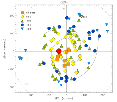
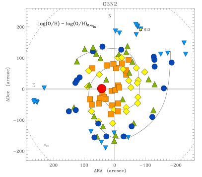
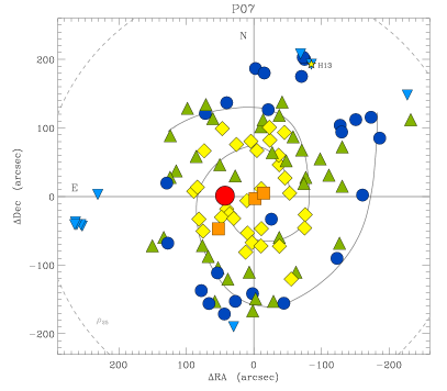
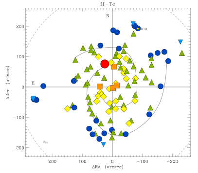
Figure 19: 2D distribution of the oxygen abundances derived from the IFS H II regions catalogue of NGC 628 (plus selected H II regions from the literature), for the KK04 (top-left), $O3N2$ (top-right), P07 (bottom-left) and ff-Te (bottom-right) metallicity calibrators. The shape and colours of the symbols correspond to the difference $\Delta$[12 + log(O/H)] $\equiv\Delta\log(\rm{O/H})$ between the abundance obtained on each H II region with respect to the characteristic abundance $12+\log(\rm{O/H})_{\rho=0.4\rho_{25}}$ of the same calibrator, grouped in bins of $0.0,\pm 0.1,0.2$ dex (e.g. +0.1 dex = $0.05\leq\Delta\log(\rm{O/H})<0.15$). The large symbol in red colour stands for the location of the H II region with the maximum amount of 12 + log(O/H) measured for that calibrator. The position of the H13 region mentioned in the text is shown as a yellow-star. The grey-thick lines define the operational spiral arms of the galaxy. The dotted-circle corresponds to the size of the optical radius $\rho_{25}$. See the text for more explanation.

The 2D spectroscopic view of NGC 628 offer us the opportunity to go beyond a simple radial abundance gradient, we are now in the position to test whether the metal abundance distributions in the disc are axisymmetric (factor which is usually taken for granted in chemical evolution models), to locate chemical enhanced regions, areas in which the physical conditions of the gas differ with respect to morphologically similar or axisymmetric regions, and the possible relations of these properties with dynamical features. NGC 628 is a nearly face-on galaxy ($i=24$^∘) with a well-defined disc, geometric variations of its physical and chemical properties might be sought by partitioning the area of the galaxy in different sectors and/or by comparing the trends and results of the different abundance indicators at difference sectors.

For this analysis, we took as a base the spectroscopic data corresponding to the IFS H II regions catalogue of NGC 628 plus H II regions from the literature with $\rho\gtrsim\rho_{25}$. The positions of the H II regions were deprojected in order to account for any geometric bias imposed by the small inclination of the galaxy. Fig. 19 shows a 2D distribution of the oxygen abundances for the four strong-line abundance calibrators considered in the previous section. The shape-colour coding corresponds to the difference $\Delta$[12 + log(O/H)] $\equiv\Delta\log(\rm{O/H})$ between the abundance measured on each H II region with respect to the characteristic abundance $12+\log(\rm{O/H})_{\rho=0.4\rho_{25}}$ of the same calibrator as listed in Table 3 (which nearly coincides with the metallicity derived from the integrated spectrum of the galaxy), grouped in bins of $0.0\pm 0.1,0.2$ dex (e.g. +0.1 dex = $0.05\leq\Delta\log(\rm{O/H})<0.15$). The large circle in red colour stands for the location of the H II region in which the maximum metallicity was measured for that calibrator. The figure shows the operational spiral arms as defined in Fig. 9 (grey-thick lines), the optical size of the galaxy $\rho_{25}$ (dotted-circle) and as a yellow-star the position of the H13 region described above. This representation of the abundance distribution might be particularly useful in order to examine the 2D metallicity structure as derived by a particular abundance calibrator, to detect chemical enhanced regions, or to compare the metallicity distribution with the morphology of the galaxy and with other metallicity indicators, bearing in mind that this can be performed only in statistical terms, given the well-known uncertainties of the strong-line abundance indicators. Nevertheless, this rendering may still be useful when describing the overall structure of the 2D metallicity distribution for a given calibrator.

Direct comparison between these abundance renderings show that the 2D metallicity structure varies between the different metallicity calibrators. Whereas we find many regions with $\Delta\log$(O/H) = +0.2 dex with the KK04 and $O3N2$ indicators, the P07 and ff–$T_{e}$ calibrations show very few (which explains the flatter slopes of the two latter distributions on Fig. 14). An important point to note is that in all cases the maximum log(O/H) value is not found at the centre of the galaxy, in the case of KK04, $O3N2$ and P07, the location of the maximum abundance it is displaced $\sim 45$ arcsec ($\sim 2$ kpc) to the east with respect to the morphological centre of the galaxy, while for the f-$T_{e}$ calibrator the point of maximum abundance is different, being found some $\sim 60$ arcsec ($\sim 3$ kpc) north of the centre. The distribution of regions with similar $\Delta\log$(O/H) are also different, in the case of the KK04 calibrator the regions of enhanced abundance are located at the central south-east region of the galaxy, while in the case of the $O3N2$ calibrator, the enhanced regions are morphologically linked to the central sections of both spiral arms. In the case of the P07 and ff–$T_{e}$ calibrators, the 2D abundance structures are somewhat similar (with the exception of the maximum log(O/H) H II region). Note that the 2D rendering of the abundance distribution of NGC 628 has shown information that is usually lost in a simple radial abundance gradient, and that might be relevant when constructing a chemical evolution model based on a particular abundance determination.

As a second exercise using the 2D information of NGC 628, we divided the galaxy in four quadrants with respect to an arbitrary axis, considering the abundance analysis of Section 3.2 for each sector separately. Then, we looked for variations or dissimilar trends between the different sectors in diagnostic diagrams, line-ratios as a function of deprojected galactocentric radii, and metal abundance gradients for different calibrators. We performed this exercise for different values of the position angle (PA₀) of the arbitrary axis from which the galaxy quadrants were defined, ranging from PA₀=0 to 90^∘, in 5^∘steps.

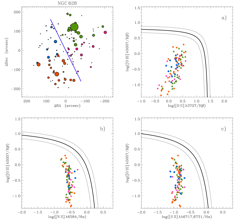
Figure 20: Top-left panel: deprojected spatial distribution of the selected H II regions of NGC 628 grouped according to their geometric position (quadrant) with respect to the blue axis drawn across the galaxy surface (PA₀ = 25^∘). H II regions belonging to the 1st quadrant (i.e. 0^∘$\leq$ PA $<$ 90^∘with respect to the main axis) are coded as blue, regions in the 2nd quadrant (90^∘$\leq$ PA $<$ 180^∘) are drawn in orange, regions of the 3rd quadrant (180^∘$\leq$ PA $<$ 270^∘) in magenta, and those of the 4th quadrant (270^∘$\leq$ PA $<$ 360^∘) in green. The size of the circles defining an individual H II region corresponds to the “aperture” dimension as defined in Section 4. Panels a), b) and c) show diagnostic diagrams for these H II regions coded according to the quadrants as follows: 1st: blue-circles, 2nd: orange-squares, 3rd: magenta-diamonds, 4th: green-triangles.

The top-left panel of Fig. 20 shows the deprojected spatial distribution of the selected H II regions of NGC 628. The size of the circles defining an individual H II region corresponds to the “aperture” dimension as defined in Section 4. The H II regions have been grouped in different colours corresponding to the geometric position (quadrant), with respect to the axis at which the more noticeable variations between the physical properties of the different sectors were found (see below). The PA₀ of this particular axis is 25^∘(drawn across the galaxy surface). H II regions belonging to the first quadrant (i.e. 0^∘$\leq$ PA $<$ 90^∘with respect to the main axis PA₀) are coded as blue, regions in the second quadrant (90^∘$\leq$ PA $<$ 180^∘) are drawn in orange, regions of the third quadrant (180^∘$\leq$ PA $<$ 270^∘) in magenta, and those of the fourth quadrant (270^∘$\leq$ PA $<$ 360^∘) in green.

Panels a), b) and c) of Fig. 20 show similar diagnostic diagrams as those introduced in Section 3.1. The colour of the regions correspond to the different quadrants as explained above, different symbols have been used in order to easily discriminate between the different sets of data (1st quadrant: circles, 2nd quadrant: squares, 3rd quadrant: diamonds, 4th quadrant: triangles). In the case of these diagnostic diagrams, the locus of different sectors do not show a clear trend or do not populate a clearly visible region on any diagram, compared to the rest of the quadrants. Points from all the regions are equally distributed within the cloud of points on each diagnostic diagram. However, some minor features are noticeable in some cases, for example in Panel a) the regions belonging to the 1st quadrant (blue-circles) do not seem to show gradient in the value of [O II] $\lambda$3727/H$\beta$ as the rest of the sectors, i.e. the log([O II]/H$\beta$) ratio for the 1st quadrant shows a restricted range of values ($\sim 0.0$ to 0.5 dex), while for the rest of the sectors, the same ratio ranges for more than an order of magnitude (log([O II]/H$\beta$) $\sim-0.5$ to 0.7 dex). The range of [O III]$\lambda$5007/H$\beta$ values for the 1st quadrant is also shorter, compared to the rest of the sectors, comprising only values between log([O III]/H$\beta$) $\sim-0.9$ to 0.0 dex, while for example, the 2nd and 4th quadrants range from $\sim-1.5$ to 0.3 dex. One possible reason of the restricted range in the [O II] and [O III]/H$\beta$ ratios for the 1st quadrant might be a simple statistical bias, considering the relative low number of H II regions sampled within that sector (16), compared to the regions in the 2nd and 4th quadrants (33 and 30 respectively), and that the range of galactocentric distances of the H II regions within this sector is restricted, excluding regions close to the nucleus of the galaxy (with typically low [O II] and [O III]/H$\beta$ ratios) and far for it (with higher ratios of the same lines).

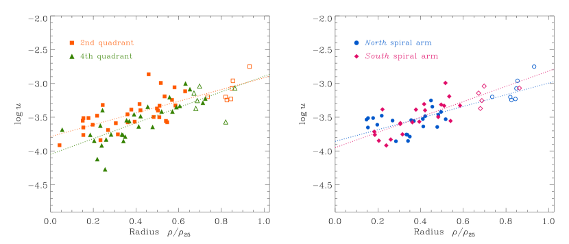
Figure 21: Radial gradients of the ionization parameter $\log u$ for geometrical and morphologically selected H II regions of NGC 628. The left panel shows the $\log u$ vs. $\rho$ relation for the regions of the 2nd and 4th quadrants of the galaxy as defined in Fig. 20. The right-panel shows the same relation for the regions belonging to the North and South spiral arms as defined in the text.

As mentioned above, the [N II] $\lambda$6584/H$\alpha$ and [S II] $\lambda$$\lambda$6717,31/H$\alpha$ ratios shown in Panels b) and c) do not show any clear trend among the different sectors, apart from the difference in the oxygen ranges discussed before. Other typical diagnostic diagrams were explored with similar finding, i.e. the locus of the different sectors are spread among the overall scatter showing no clear trends. Following the course of action of the previous sections, we explored possible variations among the different sectors in the emission line intensities and derived properties as function of galactocentric radius, similarly to Fig. 7 and Fig. 11. The most discernible variation was found in terms of the ionization parameter $\log u$ (which is equivalent to the excitation diagnostic [O III]/[O II]). The left-panel of Fig. 21 shows the values of the ionization parameter as function of galactocentric radius for those H II regions within the 2nd and the 4th quadrant only. The other sectors were not included for the sake of clarity and in order to stress the differences between these two samples. Furthermore, the 2nd and 4th quadrants include most of the largest and brightest H II regions in the galaxy, they are the most populated sectors in terms of the total number of individual H II regions, they contain the whole range of galactocentric distances of both the IFS observations (filled symbols) and the H II regions from the literature which were identified to belong to a certain section (open symbols), sampling geometrically symmetric regions of the galaxy [see Panel a) of Fig. 20].

Visually, the values of the ionization parameter found in the 2nd quadrant seem to be higher than those found in the 4th sector, and with a different level of variation as function or galactocentric radius, i.e. the gradient of the ionization parameter on the 4th quadrant is steeper than one found at the opposite side of the galaxy. The dotted lines in Fig. 21 represent a linear fit to each of the samples, in the case of the 2nd sector, the value of $\log u$ at $\rho_{0}$ is $-3.8\pm 0.06$, with a slope of $0.87\pm 0.12$ dex $\rho_{25}^{-1}$, while for the 4th quadrant, $\log u$ at $\rho_{0}$ is equal to $-4.1\pm 0.08$, with a slope of $1.15\pm 0.16$ dex $\rho_{25}^{-1}$. Although the differences in the central $\log u$ and slope of the gradients for the two samples are not extreme, they do indicate a different behavior of the ionization parameter in these two opposite regions of the galaxy. In fact, a two-sided Kolmogorov-Smirnov test applied to the distributions of the two samples yields a probability of 11% that two arrays of data values are drawn from the same distribution. The two innermost points of the figure at $\rho<0.1\rho_{25}$ do not seem to visually follow this behavior. However, given their proximity between them and to the centre of the galaxy, the segregation of these regions into different “geometrical quadrants” might not be relevant. Nevertheless, the inclusion of these points does not affect the general results of the linear fitting and the trends discussed above.

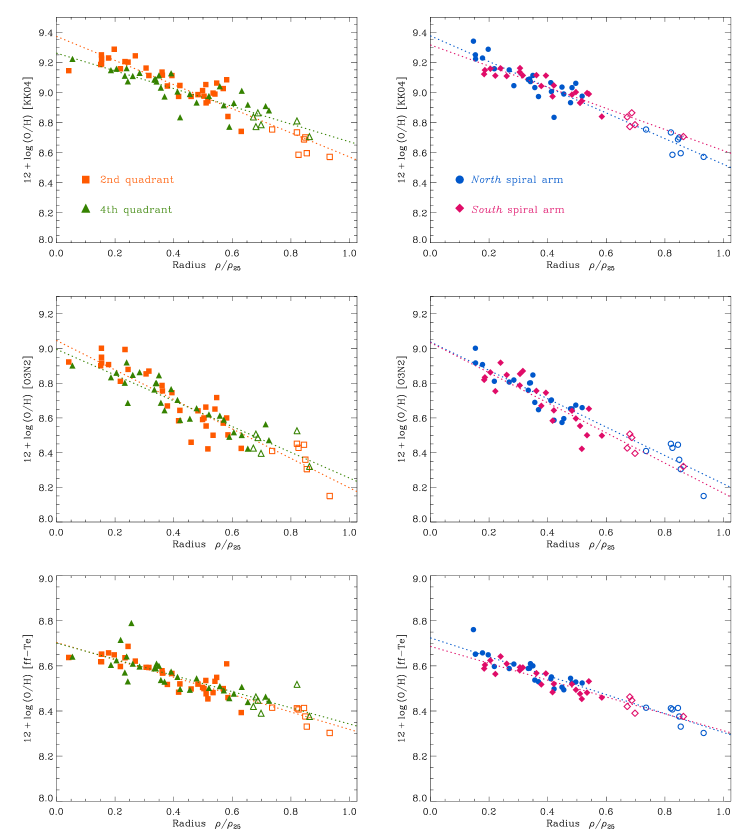
Figure 22: Radial abundance gradients of NGC 628 based on geometrical and morphologically selected H II regions. Top-panels: Oxygen gradient derived after the $R_{23}$-based KK04 calibrator. Middle-panels: Oxygen gradients based on the PP04 calibrator. Bottom panels: Abundance gradients based on the ff–$T_{e}$ method. In all panels, the dotted-lines correspond to linear fits to the data.

The H II regions included in the 2nd and 4th quadrants trace a good portion of the spiral arms of NGC 628, but each of these sectors includes regions from both of the most prominent arms of the galaxy. One logical step in the 2D spectroscopic analysis of this galaxy is to test for variations in the abundance and physical properties between the spiral arms of NGC 628. For this purpose, we selected the largest and brightest H II regions along the two most prominent spiral arms sampled by the FOV of the IFS mosaic of the galaxy, as defined in Fig. 9. For the North arm, we chose the H II regions N628 6-9, 26-31, 35-43, 45, 56, 68 and 69, while for the South arm, we selected regions N628 12-15, 20, 22, 60, 65, 66, 74, 80-85, 87-88, 90-91 and 94. The regions in each spiral arm were selected to sample the closest coincident range in deprojected galactocentric distances, we also excluded regions near the centre of the galaxy in order to avoid confusions in the association to any specific arm. We also considered H II regions from the literature found to belong to a certain spiral arm, although we only included those beyond the FOV of the IFS data (open symbols). The results of the abundance analysis for each spiral arm were compared in a similar way as the analysis for the four quadrants defined above. Diagnostic diagrams, emission line ratios and derived properties were explored, seeking for any variation between the two new samples. Again, the most notorious difference was found in the values of the ionization parameter as a function of radius, as shown in the right-panel of Fig. 21. The regions belonging to the North spiral arm are coded as blue-circles, while regions from the South arm are drawn as reddish-diamonds.

The difference between the two spiral arms clearly resides in the slope of the gradient of $\log u$, for the North arm, the values of $\log u$ increase moderately with galactocentric distance, while for the South arm, the ionization parameter increases with a steeper slope. The dotted-lines represent linear fits to the data, for the North arm the $\log u$ at $\rho=0$ is $-3.86\pm 0.06$ , with a slope of $0.86\pm 0.12$ dex $\rho_{25}^{-1}$. On the other hand, the $\log u$ at $\rho_{0}$ for the South arm is $-3.95\pm 0.08$, with a slope of $1.13\pm 0.17$ dex $\rho_{25}^{-1}$. Coincidently, the linear fits of the two spiral arms intersect at a radius $\rho\sim 0.4\rho_{25}^{-1}$, with $\log u\approx-3.5$, i.e. the $\log u$ value of the integrated spectrum of NGC 628. A two-sided Kolmogorov-Smirnov test reports a probability of 36% for the two samples to be originated from the same distribution.

The positive gradient of the ionization parameter (or the [O III]/[O II] emission-line ratio) shown in Fig. 21 reflects an increase of the nebular excitation with galactocentric distance. These emission-line ratios radial trends are known since the pioneering works by Aller (1942) and Searle (1971) and are subject of different interpretations. In the scenario that the stellar excitation per nebula is more or less uniform across the galaxy (which is unlikely given the large range of physical parameters within extragalactic H II regions, e.g. density, temperature, size and the spectrum of ionizing radiation, etc.), the increase in the excitation with radius has been interpreted as an effect of the shift of the principal cooling mechanism, from infrared fine-structure transitions to optical [O III] emission in regions of lower metallicities found at larger radii, i.e. as a consequence of the metallicity gradient (see Shields, 1990, and references therein). An alternative explanation of the observed gradients in excitation (and in the EW(H$\beta$) emission) is a gradient of the mean stellar temperature of the ionizing source $T_{*}$, with the ionizing radiation becoming harder with increasing radius (Shields, 1974; Shields & Tinsley, 1976; Shields & Searle, 1978). Indeed, the effect of increase $T_{*}$ with decreasing abundance has been confirmed by different authors (e.g. Stasińska, 1980; Campbell et al., 1986; Vilchez & Pagel, 1988). However, some other authors argue that this observed trend is consistent with a single ionizing temperature and a varying nebular geometry (Evans & Dopita, 1985), or that there is metallicity-dependent IMF which translates into a differential star-formation at varying radii (Shields & Tinsley, 1976), etc. More recent synthesis models include evolving clusters which predict a softening of the stellar ionizing spectra with increasing abundance (e.g. Maeder, 1990), or that the variation on the strength of the [O III] emission-line and the ionization parameter (which is not a free-parameter) is due to the changes in the cluster mass and in the cluster age, which determines the number of ionizing photons, the overall ionization spectrum hardness and the ionized region size (Martín-Manjón et al., 2010). Although is beyond the scope of this paper, comparison of these models with the 2D IFS data of H II regions is necessary in order to discriminate the different possible scenarios.

The top-panels of Fig. 22 show the abundance gradient of NGC 628 for the 2nd and 4th sectors as defined in Fig. 20, and the two spiral arms H II regions samples introduced previously for the $R_{23}$-based KK04 calibrator, following the same style prescriptions as before. Linear fits to each data sample are represented by dotted-lines. The effect of the different gradient of the ionization parameter is evident in these two panels. In the first case, the metallicity gradient derived for the 2nd quadrant of NGC 628 shows slightly higher oxygen values than those calculated for the 4th quadrant. The central oxygen value for 2nd sector is 12 + log(O/H) = 9.37 $\pm 0.03$, while for the 4th sector is 9.26 $\pm 0.02$. The slope for the 2nd quadrant is much steeper ($-0.82\pm 0.05$ dex $\rho_{25}^{-1}$) than for the 4th sector ($-0.58\pm 0.06$ dex $\rho_{25}^{-1}$). In the case of the spiral arms, the independent metallicity gradients for each sample are also clearly distinct. The North spiral arm shows a steeper gradient ($-0.85\pm 0.05$ dex $\rho_{25}^{-1}$), consistent with a higher central oxygen abundance (12 + log(O/H)₀ = 9.38 $\pm 0.02$), while the abundance gradient for the South arm shows a flatter slope ($-0.70\pm 0.04$ dex $\rho_{25}^{-1}$), a lower central abundance (12 + log(O/H)₀ = 9.31 $\pm 0.03$), but most importantly, a practically flat oxygen distribution for regions at $\rho<0.3\rho_{25}$.

The middle and bottom-panels of Fig. 22 show the oxygen metallicity gradients of the samples discussed above for the $O3N2$ calibration and the ff–$T_{e}$ method, respectively. In the case of the $O3N2$ calibration, the left, middle-panel shows different slopes for the 2nd and 4th quadrants, with the same behavior than the KK04 calibrator, i.e. a steeper gradient for the 2nd sector; while in the right, middle-panel the H II regions corresponding to the North spiral arm are consistent with a well-defined gradient with a steep slope at all galactocentric distances, with a coincident central abundance a nearly equal slopes. In the case of the ff–$T_{e}$ method, the distribution of data points in both cases are equally scattered at all galactocentric distances in each panel the distributions of the H II regions show a tight similarity, evident also through the linear fits applied to the individual samples. However, the South arm sample show the same behavior as in the case of the KK04 index, i.e. a decreasing gradient for the outer regions, and a flat distribution for the inner regions ($\rho\leq 0.35\rho_{25}$), suggesting a flat oxygen abundance distribution of 12 + log(O/H) $\sim$ 8.6.

In summary, although the variations between the central oxygen abundances and slopes for both, the geometrical (quadrants) and morphological (arms) regions of the galaxy fall within the expected errors of strong-lines empirical calibrators, the radial trends in the ionization parameter and metallicity abundances are somewhat distinct, indicating that to a certain extent, the physical conditions and the star formation history of different-symmetric regions of the galaxy have evolved in a slightly different manner.

6 Summary and conclusions

The IFS analysis of NGC 628 was taken as a case study in order to explore different spectra extraction and analysis methodologies, taking into account the signal-to-noise of the data, the 2D spatial coverage, the physical meaning of the derived results, and the final number of analysed spectra. The proposed methods differ mainly in the way to select a subsample of spectra from the IFS mosaics, from which a spectroscopic analysis can be later performed. The selection criteria of the first method, the fibre-by-fibre sample, proved to select regions with good quality spectra from which different physical properties of the gas were derived, although with a high level of scatter. This method was also able to identify regions of interstellar diffuse emission. The second extraction method consisted in creating a catalogue of “classical” H II regions from a purely geometrical principle, i.e. by co-adding (by visual selection) fibres considered to belong to the same morphological region. Quality and sanity checks were applied in both methods, seeking for only those regions with meaningful spectral features. A combination of these methods was used in order to perform the 2D spectroscopic analysis of NGC 628. The locus of the selected spectra was explored by employing typical diagnostic diagrams of reddening corrected emission line ratios.

General results inferred from the different spectroscopic selection methods are the following:

1. Despite the large number of spectra contained in the original observed mosaic of NGC 628, the final number of fibres containing analysable spectra of enough signal-to-noise for a spectroscopic study of the ionized gas represents only a reduced percentage of the total number of fibres contained in the full IFS mosaic. For this particular case, less than 10% of the total area sampled by the IFU observations is considered of sufficient quality.

2. The “non-physical” [O III] $\lambda$5007/$\lambda$4959 line ratios found in the final samples of the fibre-by-fibre and H II region catalogues are due to errors introduced by the subtraction of the stellar population contribution to the data, the effect is especially important in regions of weak emission in the [O III] lines (e.g. the centres of the galaxies). Therefore, although the [O III] ratio may not be close to the theoretical value, the combination of their derived line ratios are still representative of the physical conditions and metallicity abundance.

3. The comparison between the line-ratio trends derived from the fibre-by-fibre sample and those of the H II region catalogue shows that, the selection criteria applied to the former case resulted in regions that follow, in statistical basis, exactly the same patterns and trends provided by the more “refined” H II region sample, although with a larger level of scatter.

4. In both cases, the selected spectra were consistent with emission produced by ionization due to a thermal continuum, i.e. hot OB stars. The radial variation of the $R_{23}$ metallicity indicator, the ionization parameter and the [N II] $\lambda$6584/H$\alpha$ ratio were also analysed, showing clear trends.

It is important to mention that, during the analysis process described in this paper, special attention was paid in order to avoid an over-automatization that could lead to errors in the derived physical parameters from the resultant spectra. Given the large amount of data, some problems might be expected for individual fibres, pointings or regions, or in the derived quantities from the measured line intensities. However, all the quality checks performed to the data (and the results derived from them) suggest that the methodology implemented in this work is very advantageous for a statistical and comparative study, and when dealing with a large number of spectra.

Once the quality and physical meaning of the spectra samples were verified, we proceeded to perform a chemical abundance analysis of the nebular emission of the galaxy. A suite of strong-line metallicity indicators were employed in order to derive the oxygen abundance radial gradients of NGC 628 for the different sets of spectra. The results were compared among them in a statistical basis. H II regions from the literature were incorporated to the PINGS H II region catalogue in order to increase the baseline for the derivation of the abundance gradients. Likewise, the emission line ratios and metallicity abundance of 9 H II regions from the literature within the FOV of the IFS mosaic of NGC 628 were compared to the observations of this work, with an overall agreement. Furthermore, a “classical” abundance gradient determination was also performed, by selecting large and bright H II regions, the results are consistent (within the errors) with the values derived from the analysis of the full H II region distribution.

The most important results derived from the 2D IFS emission-line analysis of NGC 628 are the following:

1. By comparing the results of the different abundance calibrators, we found that the metallicity distribution of NGC 628 is consistent with a nearly flat-distribution in the innermost regions of the galaxy ($\rho/\rho_{25}<0.2$), a steep negative gradient for $0.2\lesssim\rho/\rho_{25}<1$, and a shallow or nearly-constant distribution beyond the optical edge of the galaxy, i.e. implying a multi-modality of the abundance gradient of NGC 628. The same feature is observed for the N/O vs. $\rho$ distribution. The existence of this feature may be related to the differences in the 2D gas surface density and star formation rate between the inner and outer disc which inhibits the formation of massive stars in the outer regions, causing a lack of chemical evolution in the outer disc compared with the inner regions.

2. The observed dispersion in the metallicity at a given radius for the fibre-by-fibre sample is neither a function of spatial position, nor due to low S/N of the spectra, and shows no systematic dependence with the ionization conditions of the gas, implying that the dispersion is real, and is reflecting a true spatial physical variation of the oxygen content.

3. Considering that the observed H$\alpha$ luminosity corresponds to that expected for relatively large H II regions (in which the flux of ionizing photons is produced by stellar clusters with the necessary mass to overcome problems due to stochastic effects), the determination of the metallicity abundance through the strong-line indicators can be considered reliable for both the fibre-by-fibre and H II region samples, as the derived metallicity does not depend importantly on the ionization conditions of the emitting gas.

4. The values of the oxygen abundance derived from the integrated spectrum for each calibrator equal the abundance derived from the radial gradient at a radius $\rho\sim 0.4\rho_{25}$, confirming for this galaxy previous results obtained for other objects, i.e. that the integrated abundance of a normal disk galaxy correlates with the characteristic gas-phase abundance measured at $\rho\sim 0.4\rho_{25}$.

5. By constructing 2D maps of the oxygen abundance distributions, we found that the 2D metallicity structure of the galaxy varies depending on the metallicity calibrator employed in order to derive the oxygen abundance. Different calibrators find regions of enhanced log(O/H) at spatial positions which are not coincident among them. This implies that the use of different empirical calibrations do not only reflect in a linear scale offset, but may introduce spurious inhomogeneities. This information is usually lost in a simple radial abundance gradient, and that might be relevant when constructing a chemical evolution model based on a particular abundance determination.

6. While trying to find axisymmetric variations of the metallicity content in the galaxy, we found slight variations between the central oxygen abundances and slopes for both, the geometrical (quadrants) and morphological (arms) regions of the galaxy. Although these small variations fall within the expected errors involved in strong-line empirical calibrations, the radial trends in the ionization parameter and metallicity abundances are somewhat distinct, indicating that to a certain extent, the physical conditions and the star formation history of different-symmetric regions of the galaxy have evolved in a different manner.

7. The metallicity of the gas seems to follow the trend marked by previous IFS studies of the stellar populations at the centre of the galaxy (see Paper I). This result, together with the presence of circumnuclear star-forming regions might indicate a scenario in which the gas is being radially transferred, inhibiting the enhancement of the gas-phase metallicity at the innermost regions of the galaxy.

Hitherto, most spectroscopic works have obtained abundance gradients by observing only a few, large and bright H II regions over the surface of the galaxies. However, the body of results presented in this work were obtain (to a good extent) thanks to the fact that we benefit from a nearly complete coverage of small and large H II regions observed over the surface of the galaxy, which gives us the possibility to explore the systematics between different ways of obtaining the abundance gradients. In particular, the results from this paper give support to the existence of flat metallicity distribution in the inner and outer parts of the discs of nearby spiral galaxies, although the definite existence (and interpretation) of these attributes will require further observations and a larger statistical sample. The capability to detect these features represent one of the powers of IFS observations. Likewise, the results also contribute to reaffirm (in a statistical way) the robustness of the strong-line methods applied to individual regions sampled by different fibre apertures, and to the integrated spectra of the whole galaxy.

The study of the nebular properties of NGC 628 presented in this paper has been restricted to include a 2D abundance analysis, focused on the spectra selection method, on the abundance gradients and variations of nebular derived properties across the surface of the galaxy. More detailed studies regarding the 2D distribution of the physical and chemical properties of this galaxy will be addressed in future papers of this series.

Appendix A On the spectra extraction methodology

In this appendix, we give further information regarding the fibre-by-fibre spectra extraction technique that was implemented during the IFS analysis of NGC 628. This method considers that the fibre aperture of the PPAK instrument samples a region which is large-enough in physical scale to be the source of an analysable spectrum. As explained in Section 3.1, the spectra extraction for the fibre-by-fibre method was performed on residual mosaic obtained after discarding all those fibres with low S/N and foreground objects. The sample selection was split in three steps, each with different quality criteria conditions based on different assumptions, explained as follows:

1. An analysable spectrum would need to include several detected lines in order to perform a basic analysis. One obvious line is H$\beta$, as the typical line ratios used in any spectroscopic analysis are normalised to the flux intensity of this line, and as it is required to derive a first-order correction for interstellar extinction based on the H$\alpha$/H$\beta$ ratio. Furthermore, a well-defined region from which we could derived physical meaningful properties would have to include both the [O III] $\lambda$4959 and $\lambda$5007 lines. The $\lambda$4959 line is weaker than the $\lambda$5007 by a theoretical factor of 2.98 (Storey & Zeippen, 2000), therefore the detection of the [O II] $\lambda$4959 line would also assure the detection of the $\lambda$5007 line. It is important to note that the detection of the $\lambda$4959 and $\lambda$5007 lines does not imply necessary their correct measurement, as discussed in Section 3.1. Given the theoretical constrain on the observed ratio of these two lines, the requirement of the detection of [O III] $\lambda$4959 (and consequently of $\lambda$5007) will help to characterise the quality of the subsample spectra and their physical meaning. Therefore, the first criterion applied to the residual mosaic was to select those fibres where both, the H$\beta$ and [O III] $\lambda$4959 line intensities were greater than zero, i.e. meaning that the lines are detected in the automated line intensity calculation. In the case of NGC 628, the total number of fibres for which this criterion was fulfilled is 2659, i.e. 38% of the 6949 fibres contained in the clean mosaic and 20% of the original number of fibres in the observed, unprocessed mosaic.

2. During the data processing of the line intensities and their subsequent manipulation into reddening corrected line flux ratios, there were found problems of non-floating numbers among the thousands of derived figures. A careful inspection showed that the reason of these values was due to an incorrect determination of the logarithmic extinction coefficient c($H\beta$) (calculated from the H$\alpha$/H$\beta$ ratio, accordingly to the prescriptions describe in Paper I), which produced Not-a-Number (NaN) or infinite values in those cases in which the intensity of the H$\beta$ line was very close to zero. Therefore, the second selection criterion considered only those fibres for which the calculated c($H\beta$) value was a finite-floating number, regardless of its value (including negative, non-physical ones). The number of fibres with non-finite c($H\beta$) values in NGC 628 accounts for 97 spectra, reducing the number of selected fibres after this step to 2562.

3. After applying the previous selection criteria, the data subsample consisted in a set of fibres with line intensities greater than zero for H$\beta$ and [O III] $\lambda$4959 and finite values of the derived c(H$\beta$). Based on the experience learned from the emission line maps analysis, an additional signal-to-noise cut had to be applied in order to obtain a subsample of spectra from which meaningful information could be obtained. As in the previous case, the flux threshold was based on the line intensity of the H$\beta$ line. The H$\beta$ flux cut was chosen instead of the probably more common H$\alpha$ because, as experience with the data manipulation proved, in some cases a certain line intensity threshold on H$\alpha$ did not mean the correct detection and measurement of H$\beta$, and a high cut in H$\alpha$ would eliminate many regions of low intensity but with physical meaning. Furthermore, as the main focus is to characterise the chemical abundance of the galaxy, we required the presence on the spectrum of typical strong lines from which we could obtain information on the abundance for a given region. Thus, a further requirement applied at this point to the spectra was the detection of the [O II] $\lambda$3727 line, given that many of the most important abundance calibrators are based on the line strength of this line (e.g. $R_{23}$, see Section 4). Therefore, the last selection criteria applied to the spectra sample obtained in the previous steps was, to select those fibres where the line intensity of the H$\beta$ line was greater than or equal to a given flux limit threshold, and that the line intensity of [O II] $\lambda$3727 was greater than zero, i.e. the emission line was detected. The flux limit applied in H$\beta$ was equal to 8 $\times$ 10^-16 erg s^-1 cm^-2. The final number of spectra after applying the last selection criteria was 376 fibres, which constitutes only $\sim$ 3% of the original spectra in the IFS mosaic of NGC 628.

Even though all the selection criteria discussed above could had been merged into a single pipeline, we decided to separate the different steps for the following reasons: 1) In order to check the number of fibres kept and removed at each step; 2) For an easier manipulation of the data in computational terms; 3) The different data sets could be analysed independently in order to check for systematic errors and trends due to the different quality selection criteria; 4) The subsample obtained after the second selection criteria was very likely to include regions of line emission of different physical properties of classical H II regions, e.g. regions of DIG.

Appendix B Online material

In this appendix, we list the data products that are made publicly available in online version as part of the IFS analysis of NGC 628 presented in this paper. The data can be accessed through the PINGS project webpage: http://www.ast.cam.ac.uk/ioa/research/pings, under the Public datasets section. The data release includes:

1. The H II region catalogue of NGC 628, including the number identification (ID) as shown in Fig. 9; the Right Ascension and Declination of the central reference point of each H II region (in sexagesimal and degree units), for the 2000 equinox; the offsets of each region, in arcsec, with respect to the reference central point of the IFS mosaic, as reported in Table 1 of Ros10, in the standard configuration with north-east positive; a “Method” column corresponding to the extraction method employed during the selection of the H II region (see Appendix A): A stands for an aperture extraction (i.e. a circular aperture of given size in arcsec), and M stands for manual extraction (i.e. fibres selected by hand); an “Aperture” value standing for the real (aperture) or equivalent (manual) extraction aperture diameter in arcsec; a “Size” column corresponding to the physical size of the H II region in parsecs, at the assumed distance to the galaxy, and the total number of fibres from which the spectra of the H II regions were extracted.

2. Reddening-corrected emission line intensities for the H II region catalogue, normalised to H$\beta$ (with 1$\sigma$ errors), including: [O II] $\lambda$3727, H$\gamma$ $\lambda$4340, H$\beta$, [O III] $\lambda$4959, [O III] $\lambda$5007, He I $\lambda$5876, [N II] $\lambda$6548, H$\alpha$, [N II] $\lambda$6584, [S II] $\lambda$6717.

3. Derived properties of the H II region catalogue, including: A_V, the logarithmic extinction coefficient c(H$\beta$) derived from the Balmer decrement, H$\beta$ flux in units 10^-16 erg s^-1 cm^-2, the H$\alpha$ luminosity, the ionization parameter $\log u$, the $R_{23}$ value, and the 12 + log(O/H) values for the four strong-line metallicity calibrators (KK04, $O3N2$, ff–$T_{e}$, P07).

References

- Aller (1942) Aller L. H., 1942, ApJ, 95, 52
- Alloin et al. (1979) Alloin D., Collin-Souffrin S., Joly M., Vigroux L., 1979, A&A, 78, 200
- Baldwin et al. (1981) Baldwin J. A., Phillips M. M., Terlevich R., 1981, PASP, 93, 5
- Balick & Sneden (1976) Balick B., Sneden C., 1976, ApJ, 208, 336
- Belley & Roy (1992) Belley J., Roy J.-R., 1992, ApJS, 78, 61
- Bresolin et al. (1999) Bresolin F., Kennicutt R. C., Garnett D. R., 1999, ApJ, 510, 104
- Bresolin et al. (2009) Bresolin F., Ryan-Weber E., Kennicutt R. C., Goddard Q., 2009, ApJ, 695, 580
- Campbell et al. (1986) Campbell A., Terlevich R., Melnick J., 1986, MNRAS, 223, 811
- Cardelli et al. (1989) Cardelli J. A., Clayton G. C., Mathis J. S., 1989, ApJ, 345, 245
- Castellanos et al. (2002) Castellanos M., Díaz A. I., Terlevich E., 2002, MNRAS, 329, 315
- Costas & Edmunds (1993) Costas M. B. V., Edmunds M. G., 1993, MNRAS, 265, 199
- de Vaucouleurs et al. (1991) de Vaucouleurs G., de Vaucouleurs A., Corwin H. G., Buta R. J., Paturel G., Fouque P., 1991, Third Reference Catalogue of Bright Galaxies (RC3), Volume 1-3, XII, 2069, Springer-Verlag, Berlin Heidelberg New York
- Diaz (1989) Diaz A. I., 1989, in Evolutionary phenomena in galaxies, Cambridge University Press, Cambridge and New York (A90-31743 13-90), 377
- Díaz et al. (2000) Díaz A. I., Castellanos M., Terlevich E., García-Vargas M. L., 2000, MNRAS, 318, 462
- Díaz et al. (2007) Díaz Á. I., Terlevich E., Castellanos M., Hägele G. F., 2007, MNRAS, 382, 251
- Dors & Copetti (2003) Dors O. L., Copetti M. V. F., 2003, A&A, 404, 969
- Ercolano et al. (2007) Ercolano B., Bastian N., Stasińska G., 2007, MNRAS, 379, 945
- Evans & Dopita (1985) Evans I. N., Dopita M. A., 1985, Astrophysical Journal Supplement Series (ISSN 0067-0049), 58, 125
- Ferguson et al. (1998) Ferguson A. M. N., Gallagher J. S., Wyse R. F. G., 1998, AJ, 116, 673
- Ganda et al. (2007) Ganda K., Peletier R. F., McDermid R. M., Falcón-Barroso J., de Zeeuw P. T., Bacon R., Cappellari M., Davies R. L., et al., 2007, MNRAS, 380, 506
- García-Rojas et al. (2006) García-Rojas J., Esteban C., Peimbert M., Costado M. T., Rodríguez M., Peimbert A., Ruiz M. T., 2006, MNRAS, 368, 253
- Garcia-Vargas et al. (1995) Garcia-Vargas M. L., Bressan A., Diaz A. I., 1995, A&AS, 112, 35
- Garnett (1990) Garnett D. R., 1990, ApJ, 363, 142
- Garnett (2002) —, 2002, ApJ, 581, 1019
- Goddard et al. (2010) Goddard Q. E., Bresolin F., Kennicutt R. C., Ryan-Weber E. V., Rosales-Ortega F. F., 2010, MNRAS, 1845
- Gonzalez-Delgado et al. (1995) Gonzalez-Delgado R. M., Perez E., Diaz A. I., Garcia-Vargas M. L., Terlevich E., Vilchez J. M., 1995, ApJ, 439, 604
- Hägele et al. (2008) Hägele G. F., Díaz Á. I., Terlevich E., Terlevich R., Pérez-Montero E., Cardaci M. V., 2008, MNRAS, 383, 209
- Hendry et al. (2005) Hendry M. A., Smartt S. J., Maund J. R., Pastorello A., Zampieri L., Benetti S., Turatto M., Cappellaro E., et al., 2005, MNRAS, 359, 906
- Henry et al. (2000) Henry R. B. C., Edmunds M. G., Köppen J., 2000, ApJ, 541, 660
- Hinshaw et al. (2009) Hinshaw G., Weiland J. L., Hill R. S., Odegard N., Larson D., Bennett C. L., Dunkley J., Gold B., et al., 2009, The Astrophysical Journal Supplement, 180, 225
- Hodge (1976) Hodge P. W., 1976, Astrophys. J., 205, 728
- Izotov et al. (2006) Izotov Y. I., Stasińska G., Meynet G., Guseva N. G., Thuan T. X., 2006, A&A, 448, 955
- Kauffmann et al. (2003) Kauffmann G., Heckman T. M., Tremonti C., Brinchmann J., Charlot S., White S. D. M., Ridgway S. E., Brinkmann J., et al., 2003, MNRAS, 346, 1055
- Kelz et al. (2006) Kelz A., Verheijen M. A. W., Roth M. M., Bauer S. M., Becker T., Paschke J., Popow E., Sánchez S. F., et al., 2006, PASP, 118, 129
- Kennicutt et al. (2003) Kennicutt R. C., Armus L., Bendo G., Calzetti D., Dale D. A., Draine B. T., Engelbracht C. W., Gordon K. D., et al., 2003, PASP, 115, 928
- Kennicutt & Hodge (1980) Kennicutt R. C., Hodge P. W., 1980, ApJ, 241, 573
- Kewley & Dopita (2002) Kewley L. J., Dopita M. A., 2002, ApJS, 142, 35
- Kewley et al. (2001) Kewley L. J., Dopita M. A., Sutherland R. S., Heisler C. A., Trevena J., 2001, ApJ, 556, 121
- Kewley & Ellison (2008) Kewley L. J., Ellison S. L., 2008, ApJ, 681, 1183
- Kobulnicky & Kewley (2004) Kobulnicky H. A., Kewley L. J., 2004, ApJ, 617, 240
- Lamareille et al. (2004) Lamareille F., Mouhcine M., Contini T., Lewis I., Maddox S., 2004, MNRAS, 350, 396
- Leitherer et al. (1999) Leitherer C., Schaerer D., Goldader J. D., Delgado R. M. G., Robert C., Kune D. F., de Mello D. F., Devost D., et al., 1999, ApJS, 123, 3
- López-Sánchez & Esteban (2010) López-Sánchez Á. R., Esteban C., 2010, A&A, 517, 85
- López-Sánchez et al. (2011) López-Sánchez Á. R., Mesa-Delgado A., López-Martín L., Esteban C., 2011, MNRAS, 411, 2076
- Lu et al. (1993) Lu N. Y., Hoffman G. L., Groff T., Roos T., Lamphier C., 1993, ApJS, 88, 383
- Maeder (1990) Maeder A., 1990, Astronomy and Astrophysics Supplement Series (ISSN 0365-0138), 84, 139
- Martin & Roy (1994) Martin P., Roy J.-R., 1994, ApJ, 424, 599
- Martín-Manjón et al. (2010) Martín-Manjón M. L., García-Vargas M. L., Mollá M., Díaz A. I., 2010, MNRAS, 403, 2012
- McCall et al. (1985) McCall M. L., Rybski P. M., Shields G. A., 1985, ApJS, 57, 1
- McGaugh (1991) McGaugh S. S., 1991, ApJ, 380, 140
- Mollá et al. (2006) Mollá M., Vílchez J. M., Gavilán M., Díaz A. I., 2006, MNRAS, 372, 1069
- Morisset et al. (2004) Morisset C., Schaerer D., Bouret J.-C., Martins F., 2004, A&A, 415, 577
- Moustakas & Kennicutt (2006) Moustakas J., Kennicutt R. C., 2006, ApJ, 651, 155
- Moustakas et al. (2010) Moustakas J., Kennicutt R. C., Jr., Tremonti C. A., Dale D. A., Smith J.-D. T., Calzetti D., 2010, arXiv, 1007, 4547
- Osterbrock & Ferland (2006) Osterbrock D. E., Ferland G. J., 2006, Astrophysics of gaseous nebulae and active galactic nuclei, University Science Books, Herndon VA, USA
- Pagel et al. (1979) Pagel B. E. J., Edmunds M. G., Blackwell D. E., Chun M. S., Smith G., 1979, MNRAS, 189, 95
- Peimbert (1967) Peimbert M., 1967, ApJ, 150, 825
- Pérez-Montero & Contini (2009) Pérez-Montero E., Contini T., 2009, MNRAS, 398, 949
- Pettini & Pagel (2004) Pettini M., Pagel B. E. J., 2004, MNRAS, 348, L59
- Pilyugin (2005) Pilyugin L. S., 2005, A&A, 436, L1
- Pilyugin (2007) —, 2007, MNRAS, 375, 685
- Pilyugin & Thuan (2005) Pilyugin L. S., Thuan T. X., 2005, ApJ, 631, 231
- Pilyugin et al. (2006) Pilyugin L. S., Thuan T. X., Vílchez J. M., 2006, MNRAS, 367, 1139
- Rosales-Ortega et al. (2010) Rosales-Ortega F. F., Kennicutt R. C., Sánchez S. F., Díaz A. I., Pasquali A., Johnson B. D., Hao C. N., 2010, MNRAS, 405, 735
- Roth et al. (2005) Roth M. M., Kelz A., Fechner T., Hahn T., Bauer S.-M., Becker T., Böhm P., Christensen L., et al., 2005, PASP, 117, 620
- Sánchez (2004) Sánchez S. F., 2004, AN, 325, 167
- Sánchez (2006) —, 2006, AN, 327, 850
- Sánchez et al. (2006) Sánchez S. F., García-Lorenzo B., Jahnke K., Mediavilla E., González-Serrano J. I., Christensen L., Wisotzki L., 2006, AN, 327, 167
- Sánchez et al. (2011) Sánchez S. F., Rosales-Ortega F. F., Kennicutt R. C., Johnson B. D., Diaz A. I., Pasquali A., Hao C. N., 2011, MNRAS, 410, 313
- Scott et al. (2009) Scott P., Asplund M., Grevesse N., Sauval A. J., 2009, ApJ, 691, L119
- Searle (1971) Searle L., 1971, ApJ, 168, 327
- Shields (1974) Shields G. A., 1974, ApJ, 193, 335
- Shields (1990) —, 1990, IN: Annual review of astronomy and astrophysics. Vol. 28 (A91-28201 10-90). Palo Alto, 28, 525
- Shields & Searle (1978) Shields G. A., Searle L., 1978, ApJ, 222, 821
- Shields & Tinsley (1976) Shields G. A., Tinsley B. M., 1976, ApJ, 203, 66
- Skillman et al. (1989) Skillman E. D., Kennicutt R. C., Hodge P. W., 1989, ApJ, 347, 875
- Stasińska (1980) Stasińska G., 1980, A&A, 84, 320
- Stasińska et al. (2008) Stasińska G., Asari N. V., Fernandes R. C., Gomes J. M., Schlickmann M., Mateus A., Schoenell W., Sodré L., 2008, Monthly Notices of the Royal Astronomical Society: Letters, 391, L29
- Stasińska et al. (2006) Stasińska G., Fernandes R. C., Mateus A., Sodré L., Asari N. V., 2006, MNRAS, 371, 972
- Storey & Zeippen (2000) Storey P. J., Zeippen C. J., 2000, MNRAS, 312, 813
- Talent (1983) Talent D. L., 1983, PASP, 95, 986
- Thuan et al. (1995) Thuan T. X., Izotov Y. I., Lipovetsky V. A., 1995, ApJ, 445, 108
- Tremonti et al. (2004) Tremonti C. A., Heckman T. M., Kauffmann G., Brinchmann J., Charlot S., White S. D. M., Seibert M., Peng E. W., et al., 2004, ApJ, 613, 898
- van Zee et al. (1998a) van Zee L., Salzer J. J., Haynes M. P., 1998a, ApJ, 497, L1
- van Zee et al. (1998b) van Zee L., Salzer J. J., Haynes M. P., O’Donoghue A. A., Balonek T. J., 1998b, AJ, 116, 2805
- Veilleux & Osterbrock (1987) Veilleux S., Osterbrock D. E., 1987, Astrophysical Journal Supplement Series (ISSN 0067-0049), 63, 295
- Verheijen et al. (2004) Verheijen M. A. W., Bershady M. A., Andersen D. R., Swaters R. A., Westfall K., Kelz A., Roth M. M., 2004, AN, 325, 151
- Vila-Costas & Edmunds (1992) Vila-Costas M. B., Edmunds M. G., 1992, MNRAS, 259, 121
- Vilchez & Pagel (1988) Vilchez J. M., Pagel B. E. J., 1988, MNRAS, 231, 257
- Wakker & Adler (1995) Wakker B. P., Adler D. S., 1995, The Astronomical Journal (ISSN 0004-6256), 109, 134
- Zaritsky et al. (1994) Zaritsky D., Kennicutt R. C., Huchra J. P., 1994, ApJ, 420, 87