Spotlighting quantum critical points via quantum correlations at finite temperatures

Abstract

We extend the program initiated in [T. Werlang et al., Phys. Rev. Lett. 105, 095702 (2010)] in several directions. Firstly, we investigate how useful quantum correlations, such as entanglement and quantum discord, are in the detection of critical points of quantum phase transitions when the system is at finite temperatures. For that purpose we study several thermalized spin models in the thermodynamic limit, namely, the XXZ model, the XY model, and the Ising model, all of which with an external magnetic field. We compare the ability of quantum discord, entanglement, and some thermodynamic quantities to spotlight the quantum critical points for several different temperatures. Secondly, for some models we go beyond nearest-neighbors and also study the behavior of entanglement and quantum discord for second nearest-neighbors around the critical point at finite temperature. Finally, we furnish a more quantitative description of how good all these quantities are in spotlighting critical points of quantum phase transitions at finite $T$, bridging the gap between experimental data and those theoretical descriptions solely based on the unattainable absolute zero assumption.

I Introduction

Quantum phase transitions (QPTs) theoretically occur at absolute zero temperature $(T=0)$ due to abrupt changes in the qualitative properties of the ground-state of a many-body system while varying its Hamiltonian Sac99 . The tuning parameter (the quantity being changed in the Hamiltonian) can be, for example, an external magnetic field or a coupling constant. By properly tuning the Hamiltonian one can reach a special point, the critical point (CP), where the ground state of the system undergoes a radical change, which strongly affects the macroscopic properties of the system. In the vicinity of a CP, a tiny change in the tuning parameter will favor one phase over the other. Since at $T=0$ there are no thermal fluctuations, these tiny changes are caused only by quantum fluctuations, whose origin can be traced back to the Heisenberg uncertainty principle. Some well-known examples of QPTs are the paramagnetic-ferromagnetic transition in some metals rowley , the superconductor-insulator transition dolgopolov , and superfluid-Mott insulator transition greiner .

Although reaching the absolute zero is impossible since it would violate the third law of thermodynamics, QPTs can be detected if one reaches temperatures near the absolute zero. More precisely, when the system’s de Broglie wavelength is greater than the correlation length of the thermal fluctuations one achieves a temperature low enough to see a QPT. In this regime thermal fluctuations are unable to excite the system from its ground state and a phase transition solely driven by quantum fluctuations is still possible to be seen.

Many theoretical tools employed in the calculation of these CPs are usually subjected to the $T=0$ restriction. Interesting examples are the behavior of bipartite lidar , multipartite oliveira , and generalized entanglement ortiz for spin chains at $T=0$. Quantum discord, a measure of all quantum correlations present in a system zurek ; Henderson , has also been widely used to characterize the CPs at $T=0$ Dil08 ; Sar09 . The extremal values and the behavior of the derivatives of these quantities can signal the existence of a CP without the knowledge of an order parameter, i.e., without the knowledge of what macroscopic quantity abruptly changes during the QPT.

All experiments involving QPTs are, nevertheless, performed at low temperatures, not at absolute zero, which forbid a direct connection between the measured data and those theoretical results developed for $T=0$. Recently, however, we have studied, in the thermodynamic limit, the XXZ Hamiltonian with no magnetic field and shown that quantum discord (QD) is able to detect CPs at finite $T$ while other thermodynamic quantities and entanglement fail in this task werPRL . For that model we have shown that the thermal quantum discord (TQD), i.e., QD computed for a system described by the canonical ensemble, possessed a characteristic behavior at the CP robust enough to survive an increasing $T$ and, therefore, spotlight a CP of a QPT at finite $T$.

Our goal in this work is to extend the study initiated in werPRL in at least two directions. We want, on one hand, to study different models to see whether or not TQD is still a good CP detector at finite $T$. We want to answer the following question: Does TQD possess a clear distinctive behavior at the CP strong enough to be seen at $T>0$? On the other hand, we want to be more quantitative in determining the ability of TQD, and other quantities such as entanglement, to correctly detect the CP of a QPT at finite $T$. How close to the actual CP are the estimated CPs obtained at finite $T$ via TQD? How do these estimated CPs at $T>0$ approach the correct CP as we decrease $T$? Those are the questions we also want to answer in this paper.

To achieve these goals, we consider here the XXZ model in the presence of an external magnetic field and the XY model in a transverse field. For both models we analyze the behavior of TQD and entanglement for $T\geq 0$ around their CPs. For the XXZ model with an external field we compare the efficiency of TQD with respect to entanglement in the detection of CPs as the temperature increases and also with other thermodynamic quantities. For the XY model we study the behavior of TQD and the entanglement of its first and second nearest-neighbors as a CP detector.

In order to make this work self-contained, we organize its presentation as follows. In Sec. II we review some concepts from information theory necessary to the construction of two measures of quantum correlations: QD and entanglement of formation (EoF). In Sec. III we discuss qualitatively and quantitatively the role of quantum correlations as a tool to detect QPTs at zero and finite temperatures in the XXZ and XY models, both with external magnetic fields. Our final remarks and conclusions are presented in Sec IV.

II Quantum Correlations

II.1 Quantum Discord

In the context of classical information theory nielsen , correlation is a measure of the dependence between two or more random variables or observed data values. The total correlation between two random variables $A$ and $B$ with probability distribution $p_{a}$ and $p_{b}$, respectively, is given by the mutual information (MI) nielsen

$$\mathcal{I}_{1}(A:B)=\mathcal{H}(A)+\mathcal{H}(B)-\mathcal{H}(A,B),$$ (1)

where $\mathcal{H}(X)=-\sum_{k}p_{x}\log_{2}p_{x}$ is the Shannon entropy with $p_{x}$ the probability distribution of the random variable $X$. If $p_{a,b}$ denote the joint probability distribution of the variables $A$ and $B$ then the joint entropy $\mathcal{H}(A,B)$ can be written through the Bayes’ rule $p_{a|b}=p_{a,b}/p_{b}$ bayes as $\mathcal{H}(A,B)=\mathcal{H}(A|B)+\mathcal{H}(B)$, where the conditional entropy $\mathcal{H}(A|B)=-\sum_{a,b}p_{a,b}\log_{2}p_{a|b}$ quantifies how much uncertainty is left on average about $A$ when one knows the values of $B$. Note that the conditional entropy is always non-negative and not necessarily a symmetric quantity, i.e., $\mathcal{H}(A|B)$ may be different from $\mathcal{H}(B|A)$. Using this relation between $\mathcal{H}(A,B)$ and $\mathcal{H}(A|B)$ we can obtain an equivalent version for the MI as given in (1),

$$\mathcal{I}_{2}(A:B)=\mathcal{H}(A)-\mathcal{H}(A|B).$$ (2)

For a quantum bipartite system $AB$ described by the density operator $\rho_{AB}$, a measure of their total correlation is obtained directly from Eq. (1) replacing the Shannon entropy by the von-Neumann entropy, $\mathcal{S}(X)=\mathcal{S}(\rho_{X})=-\mbox{Tr}\left(\rho_{X}\log_{2}\rho_{X}\right)$, i.e., $\mathcal{I}^{q}_{1}(A:B)=\mathcal{S}(A)+\mathcal{S}(B)-\mathcal{S}(A,B)$. However, a quantum analog of the second version of MI, Eq. (2), cannot be obtained so easily because Bayes’ rule are not always valid in the quantum case peres . For example, assuming the validity of this rule, the quantum conditional entropy would be defined as $\mathcal{S}(A|B)=\mathcal{S}(A,B)-\mathcal{S}(B)$. But this definition implies a negative value for $\mathcal{S}(A|B)$ if one computes it for the quantum state $\left|\psi\right\rangle=\left(\left|00\right\rangle+\left|11\right\rangle\right)/\sqrt{2}$, showing that this quantity cannot be interpreted as in the classical case, where it is always positive.

To ensure that the quantum conditional entropy has the same meaning as in the classical case, Henderson and Vedral Henderson defined the conditional entropy as $\mathcal{S}_{q}(A|B)\equiv\min_{\left\{M_{b}\right\}}\sum_{b}p_{b}\mathcal{S}(A|B=b)$ such that the minimization is given over generalized measurements $\left\{M_{b}\right\}$ nielsen , with $\sum_{b}M_{b}=\bm{1}_{B}$, $\bm{1}_{B}$ the identity operator that acts on $B$, $M_{b}\geq 0$ for all $b$, and $\mathcal{S}(A|B=b)=\mathcal{S}(\rho_{A|b})$ where

$$\rho_{A|b}=\frac{1}{p_{b}}(\bm{1}_{A}\otimes M_{b})\rho_{AB}(\bm{1}_{A}\otimes M_{b}),$$

with $p_{b}=\mbox{Tr}\left[(\bm{1}_{A}\otimes M_{b})\rho_{AB}(\bm{1}_{A}\otimes M_{b})\right]$. The expressions $\mathcal{S}_{q}(A|B)$ and $\mathcal{S}(A|B)$ coincide with $\mathcal{H}(B|A)$ for classical systems. Using $\mathcal{S}_{q}(A|B)$ the second quantum version for MI, Eq. (2), can be written as $\mathcal{I}^{q}_{2}(A:B)=\mathcal{S}(A)-\mathcal{S}_{q}(A|B)$. The difference between these two versions of quantum mutual information,

$$D(A|B) \equiv \mathcal{I}^{q}_{1}(A:B)-\mathcal{I}^{q}_{2}(A:B),$$ (3)

$$= \mathcal{S}(B)-\mathcal{S}(A,B)+\mathcal{S}_{q}(A|B),$$

was called quantum discord by Ollivier and Zurek zurek and interpreted as a measure of total quantum correlation. The notation $D(A|B)$ indicates that the measurements were performed on the subsystem $B$. When $\mathcal{S}(A)=\mathcal{S}(B)$ we have $D(A|B)=D(B|A)=D\left(\rho_{AB}\right)$ and therefore the QD is a symmetric quantity. As demonstrated recently ved01 the state $\rho_{AB}$ has $D(A|B)=0$ if, and only if, there exists a von Neumann measurement $\left\{\Pi_{j}^{B}\right\}$ such that $\rho_{AB}=\sum_{j}\left(\bm{1}_{A}\otimes\Pi_{j}^{B}\right)\rho_{AB}\left(\bm{1}_{A}\otimes\Pi_{j}^{B}\right)$ footnote1 . Therefore, a state $\rho_{AB}$ with $D=0$ has necessarily the form $\rho_{AB}=\sum_{j,k}p_{j,k}\left|\psi_{j}\right\rangle\left\langle\psi_{j}\right|\otimes\left|\phi_{k}\right\rangle\left\langle\phi_{k}\right|$ with $\sum_{j,k}p_{j,k}=1$ and $\left\{\left|\psi_{j}\right\rangle\right\}$ and $\left\{\left|\phi_{k}\right\rangle\right\}$ sets of orthogonal states. The states with $D=0$ are completely classically correlated in the sense of cstates . An example of such state is $\rho_{AB}=\left(\left|0\right\rangle\left\langle 0\right|\otimes\left|0\right\rangle\left\langle 0\right|+\left|1\right\rangle\left\langle 1\right|\otimes\left|1\right\rangle\left\langle 1\right|\right)/2$. This result shows that the existence of quantum correlations is due to the principle of superposition that allows describing a system through a set of non-orthogonal states. Here, and analogously to entanglement computed for thermal states arnesen , we use the nomenclature coined in Wer10 , namely, thermal quantum discord (TQD), to refer to QD computed for states described by the canonical ensemble.

The main difficulty in the determination of a closed expression for QD lies in the complicated minimization procedure for calculating the conditional entropy $\mathcal{S}_{q}(A|B)$. For two-qubit systems the minimization over generalized measurements is equivalent to a minimization over projective measurements (von Neumann measurements) minDIS . In this case, the minimization procedure can be done numerically for general two-qubit states numDIS while an analytical expression can be obtained only for a subclass of the so-called X-states (see Appendix). In this paper we employed both strategies, i.e., numerical minimization and, when available, closed expressions for computing QD.

II.2 Entanglement

Next, we introduce an important kind of quantum correlated states, the entangled states. A quantum bipartite state described by $\rho_{AB}$ is said to be entangled if, and only if, it cannot be written as a separable state $\rho_{AB}=\sum_{j}p_{j}\rho_{j}^{A}\otimes\rho_{j}^{B}$, where $p_{j}>0$ and $\sum_{j}p_{j}=1$ Wer89 ; entangle . Although there are states with non-zero quantum discord created only by local operations and classical communication (LOCC), entanglement cannot be generated in this way Wer89 . For pure states all quantum correlated states are entangled. The situation is more complicated in the case of mixed states. For example, the Werner state $\rho_{w}=\alpha\left|\psi^{-}\right\rangle\left\langle\psi^{-}\right|+(1-\alpha)\bm{1}/4$, with $\left|\psi^{-}\right\rangle=\left(\left|01\right\rangle-\left|10\right\rangle\right)/\sqrt{2}$ and $\alpha\in[0,1]$, is separable for $\alpha<1/3$ and non-local (violates a Bell-like inequality) for $\alpha>1/\sqrt{2}$. However, the Werner state have null quantum discord only for $\alpha=0$.

In this paper the measure of entanglement used is the Entanglement of Formation (EoF) Woo98 , which is defined as $EoF(\rho_{AB})=\min\sum_{j}p_{j}\mathcal{S}(\rho_{A(B)})$, where the minimization is over all ensembles of pure states $\left\{p_{j},\left|\psi_{j}\right\rangle\right\}$ such that $\rho_{AB}=\sum_{j}p_{j}\left|\psi_{j}\right\rangle\left\langle\psi_{j}\right|$ and $\mathcal{S}(\rho_{A(B)})$ is the von Neumann entropy of the reduced state of either $A$ or $B$, $\rho_{A(B)}=\mbox{Tr}_{B(A)}\left(\rho_{AB}\right)$. The EoF quantifies, at least for pure states and asymptotically, how many singlets are needed per copy to prepare many copies of $\rho_{AB}$ using only LOCC. It is worth emphasizing that it coincides with the quantum discord when one deals with pure states. An analytic closed expression for EoF is given in the Appendix.

III Results and Discussions

III.1 The XXZ Model

The first model tackled in this paper is the one-dimensional anisotropic spin-$1/2$ Heisenberg chain (XXZ) subjected to an external magnetic field in the $z$-direction. The Hamiltonian of this model can be written as

$$H_{xxz} = J\sum_{j=1}^{L}\left(\sigma_{j}^{x}\sigma_{j+1}^{x}+\sigma_{j}^{y}\sigma_{j+1}^{y}+\Delta\sigma_{j}^{z}\sigma_{j+1}^{z}\right)$$ (4)

$$- \frac{h}{2}\sum_{j=1}^{L}\sigma_{j}^{z},$$

where $\sigma_{j}^{\alpha}$ ($\alpha=x,y,z$) are the usual Pauli matrices acting on the $j$-th site and $\sigma_{L+1}^{\alpha}=\sigma_{1}^{\alpha}$ (periodic boundary conditions). Here $h$ is the external magnetic field, $J$ is the exchange constant ($J=1$) and $\Delta$ is the anisotropy parameter. We are going to consider only the case $\Delta>0$, however the negative values $\Delta<0$ can be obtained by reversing the sign of $J$ followed by a canonical transformation YANG . The critical regime $|\Delta|\leq 1$ can be parametrized by $\Delta=\cos{\gamma}$ and the non-critical regime $|\Delta|>1$ is given by $\Delta=\cosh{\gamma}$. The thermodynamical properties are obtained through the free-energy $f=-\frac{1}{\beta}\lim_{L\rightarrow\infty}\frac{\ln{Z}}{L}$, where $Z=\mbox{Tr}\left\{\exp{\left(-\beta H_{xxz}\right)}\right\}$ is the partition function, with $\beta=1/kT$ and the Boltzmann constant $k$ is set to unity.

The free-energy is calculated by Bethe ansatz techniques and can be written as follow,

$$f=e_{0}-\frac{1}{\beta}\left(V\ast\ln{B\bar{B}}\right)(0),$$ (5)

where the ground state energy $e_{0}$ is given by

$$\frac{e_{0}}{J}=\begin{cases}\cos{\gamma}-2\frac{\sin{\gamma}}{\gamma}\int_{-\infty}^{\infty}\frac{\sinh{(\frac{\pi}{\gamma}-1)\frac{k}{2}}}{2\sinh{\frac{\pi k}{2\gamma}}\cosh{\frac{k}{2}}}dk,&0<\Delta\leq 1,\\ \cosh{\gamma}-2\sinh{\gamma}\sum_{k=-\infty}^{\infty}\frac{e^{-\gamma|k|}}{\cosh{\gamma k}},&\Delta>1,\end{cases}$$ (6)

and

$$V(x)=\begin{cases}\frac{\pi}{\cosh{\pi x}},&0<\Delta\leq 1,\\ \sum_{k=-\infty}^{\infty}\frac{e^{\mathrm{i}2kx}}{2\cosh{\gamma k}},&\Delta>1.\end{cases}$$ (7)

The symbol $\ast$ denotes convolution $f*g(x)=\int_{-a}^{a}f(x-y)g(y)dy$, where $a\rightarrow\infty$ for $0<\Delta\leq 1$ and $a=\pi/2$ for $\Delta>1$.

The auxiliary functions $b(x)$, $\bar{b}(x)$, and its simply related functions $B(x)=b(x)+1$ and $\bar{B}(x)=\bar{b}(x)+1$ are solution to the following set of non-linear integral equations KLUMPER92 ,

$$\ln{b(x)} = d_{+}(x)+\left(\!K\!\ast\!\ln{B}\right)\!(x)-\left(\!K\!\ast\!\ln{\bar{B}}\right)\!(x+\mathrm{i}\gamma),$$ (8)

$$\ln{\bar{b}(x)} = d_{-}(x)+\left(\!K\!\ast\!\ln{\bar{B}}\right)\!(x)-\left(\!K\!\ast\!\ln{B}\right)\!(x-\mathrm{i}\gamma).$$ (9)

The driving term $d_{\pm}(x)$ is given by

$$d_{\pm}(x)=\begin{cases}-2J\beta\frac{\sin{\gamma}}{\gamma}\frac{\pi}{\cosh{(\pi x/\gamma)}}\pm\frac{\beta h}{2}\frac{\pi}{\pi-\gamma},&0<\Delta\leq 1,\\ -2J\beta\sinh{\gamma}\sum_{k=-\infty}^{\infty}\frac{e^{\mathrm{i}2kx}}{\cosh{\gamma k}}\pm\frac{\beta h}{2},&\Delta>1,\end{cases}$$ (10)

and the Kernel function

$$K(x)=\begin{cases}\int_{-\infty}^{\infty}\frac{\sinh{(\pi-2\gamma)\frac{k}{2}}e^{\mathrm{i}kx}}{2\sinh{(\pi-\gamma)\frac{k\gamma}{2}}\cosh{\frac{k}{2}}}dk,&0<\Delta\leq 1,\\ \sum_{k=-\infty}^{\infty}\frac{e^{-\gamma|k|}}{\cosh{\gamma k}}e^{\mathrm{i}2kx},&\Delta>1.\end{cases}$$ (11)

The system density operator $\rho$ is described by the canonical ensemble, i.e., $\rho=\exp{\left(-\beta H_{xxz}\right)}/Z$. The nearest-neighbor two-spin state is obtained by tracing all but the first two spins, $\rho_{1,2}=\mbox{Tr}_{L-2}(\rho)$. The Hamiltonian (4) exhibits both translational invariance and $U(1)$ invariance $\left(\left[H_{xxz},\sum_{j=1}^{L}\sigma_{j}^{z}\right]=0\right)$, therefore the reduced density matrix will be given by

$$\rho_{1,2}=\frac{1}{4}\left(\begin{array}[]{cccc}\rho_{11}&0&0&0\\ 0&\rho_{22}&\rho_{23}&0\\ 0&\rho_{23}&\rho_{22}&0\\ 0&0&0&\rho_{44}\\ \end{array}\right),$$ (16)

where

$$\rho_{11} = 1+2\left\langle\sigma^{z}\right\rangle+\left\langle\sigma_{1}^{z}\sigma_{2}^{z}\right\rangle,$$

$$\rho_{22} = 1-\left\langle\sigma_{1}^{z}\sigma_{2}^{z}\right\rangle,$$

$$\rho_{44} = 1-2\left\langle\sigma^{z}\right\rangle+\left\langle\sigma_{1}^{z}\sigma_{2}^{z}\right\rangle,$$

$$\rho_{23} = 2\left\langle\sigma_{1}^{x}\sigma_{2}^{x}\right\rangle.$$

The magnetization and the two-point correlations above are obtained in terms of the derivatives of the free-energy NLIE

$$\left\langle\sigma^{z}\right\rangle = -2\partial_{h}f,$$ (17)

$$\left\langle\sigma_{j}^{z}\sigma_{j+1}^{z}\right\rangle = \partial_{\Delta}f/J,$$ (18)

$$\left\langle\sigma_{j}^{x}\sigma_{j+1}^{x}\right\rangle = \frac{u-\Delta\partial_{\Delta}f+h\left\langle\sigma^{z}\right\rangle}{2J},$$ (19)

$$\left\langle\sigma_{j}^{z}\sigma_{j+1}^{z}\right\rangle = \left\langle\sigma_{j}^{x}\sigma_{j+1}^{x}\right\rangle=\frac{u+h\left\langle\sigma^{z}\right\rangle}{3J},~{}~{}\Delta=1,$$ (20)

where $u=\partial_{\beta}(\beta f)$ is the internal energy.

Using (16) we can obtain analytical expressions for TQD and EoF between two nearest-neighbor spins through Eqs. (39) and (40), respectively. See Appendix for details.

As discussed in TAKAHASHI , the XXZ model has two CPs in the absence of external field ($h=0$). An infinite-order transition at $\Delta=1$, with the ground state changing from an XY-like phase ($-1<\Delta<1$) to an Ising-like antiferromagnetic phase for $\Delta>1$, and a first-order transition at $\Delta=-1$, from a ferromagnetic phase ($\Delta<-1$) to the critical antiferromagnetic phase ($-1<\Delta<1$). In Dil08 ; Sar09 it was shown that both quantum discord and entanglement are able to detect these CPs associated to QPTs at $T=0$. In order to extend these zero temperature studies of the XXZ model, we take into account the action of the external field $h$. The effect of the external field is to shift the critical points to higher values of $\Delta$ GAUDIN . The critical point associated to the infinite-order transition $\Delta_{inf}$ is determined by the following equation

$$h=4J\sinh(\eta)\sum_{n=-\infty}^{\infty}\frac{(-1)^{n}}{\cosh(n\eta)},$$ (21)

with $\eta=\cosh^{-1}(\Delta_{inf})$, while the critical point associated to the first-order transition $\Delta_{1}$ by the equation

$$h=4J(1+\Delta_{1}).$$ (22)

Table I shows the critical points associated to first- and infinite-order QPTs for different values of the external field $h$.

Table 1: Critical points associated to the first-order QPT ($\Delta_{1}$) and to the infinite-order QPT ($\Delta_{inf}$) for different values of the external field $h$.

	$h=0$	$h=2$	$h=6$	$h=12$
$\Delta_{1}$ (first-order)	-1.00	-0.50	0.50	2.00
$\Delta_{inf}$ (infinite-order)	1.00	2.15	3.30	4.88

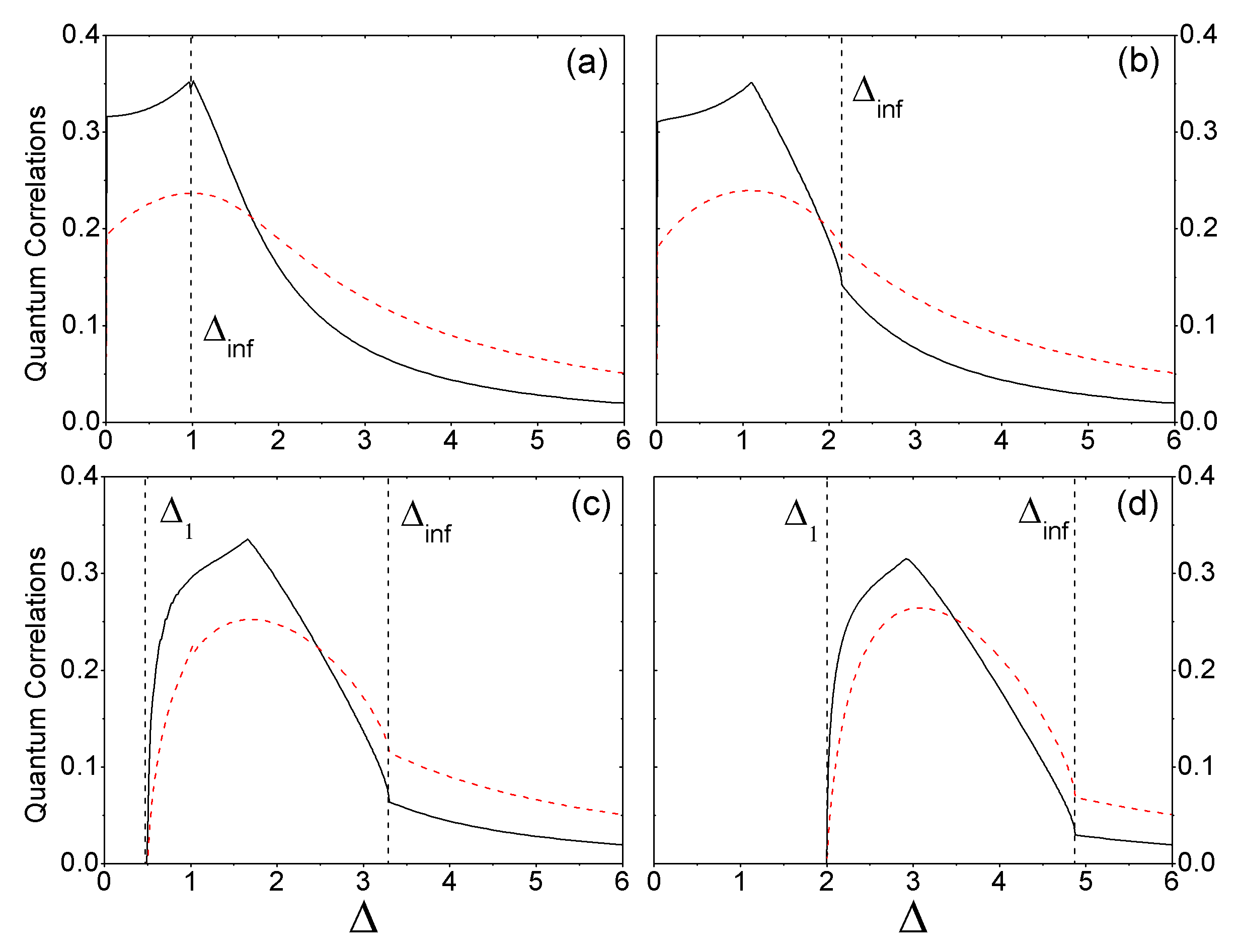
We begin our analysis by studying the behavior of TQD and EoF as a function of the tuning parameter $\Delta$ for $T=0$ and $h\geq 0$. These results are shown in Fig. 1. For $h=0$ Dil08 ; Sar09 the infinite-order transition is characterized by a global maximum of TQD and EoF at the CP $\Delta_{inf}=1$ (see Fig. 1a). But, besides being a maximum, TQD also has a cusp in this CP. This behavior implies that the first derivative of TQD is discontinuous at $\Delta_{inf}=1$ while the second derivative is divergent. For the first-order CP $\Delta_{1}=-1$ , it was shown in Sar09 that for $h=0$ the EoF and the TQD are discontinuous in the CP.

However, for $h>0$ Figs. 1b-d show that the infinite-order transition is characterized through TQD and EoF by a cusp at the CP rather than a global maximum or minimum. For a different spin model it has been recently shown rulli that the extreme points of entanglement does not necessarily indicate an infinite-order transition. Here we show an example where an infinite-order CP is pointed out not by a global maximum/minimum of the value of a quantum correlation (EoF or TQD). Rather, it is a discontinuity in its first derivative that spotlight the infinity-order QPT. Furthermore, the first-order CP $\Delta_{1}$ is well determined by TQD and EoF, as can be seen for $h=6$ (Fig. 1c) and $h=12$ (Fig. 1d). Both quantities are zero for $\Delta<\Delta_{1}$ and nonzero for $\Delta>\Delta_{1}$ while their first derivatives are divergent at $\Delta_{1}$. It is worth mentioning that the cusp-like behavior in Fig. 1 between the two CPs is due to an exchange in the set of projectors that minimizes the quantum conditional entropy werPRL , Eq. (A), and so far could not be associated with any known QPT for this model.

Figure 1: (color online) $QD$ (black solid line) and EoF (red dashed line) as functions of the tuning parameter $\Delta$ and external field $h$ for the XXZ model in the thermodynamic limit at $T=0$. (a) $h=0$, (b) $h=2$, (c) $h=6$, and (d) $h=12$. The dashed black vertical lines denote the CPs $\Delta_{1}$ and $\Delta_{inf}$. Here and in the following graphics all quantities are dimensionless.

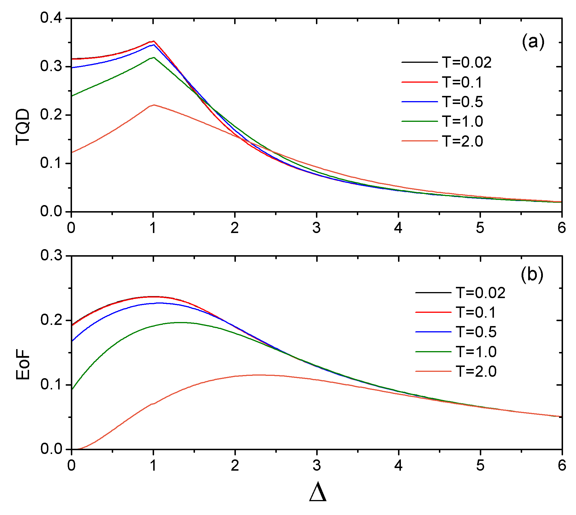
The next step is to examine how the characterization of CPs through TQD and EoF is affected by temperature when $h\geq 0$. To this end, let us start looking at the behavior of TQD and EoF for finite $T$ and $h=0$. In Figs. 2a and 2b we plot, respectively, TQD and EoF as a function of $\Delta$ for some values of $T>0$ and $h=0$. As discussed in our previous work werPRL , and illustrated in Fig. 2, for $h=0$ the first-order derivative of TQD is discontinuous at the CP $\Delta=1$ not only at $T=0$, but also at $T>0$. On the other hand, the EoF is maximum at this CP only when $T=0$ and as $T$ increases the maximum moves to higher $\Delta$ values ($\Delta>1$). The behavior of TQD in this case is related to the minimization process of the quantum conditional entropy (A). We observe that for finite $T$ there is an exchange in the functions that minimize the conditional entropy which in turn leads to a sudden change in TQD sudden , characterized by a discontinuity in its first-order derivative. It is worth noting that for $h=0$ we found a simple closed expression for TQD involving the two-point correlation functions. This closed expression together with the fact that at $\Delta=1$ we have $\left|\left\langle\sigma_{j}^{x}\sigma_{j+1}^{x}\right\rangle\right|$ $=$ $\left|\left\langle\sigma_{j}^{z}\sigma_{j+1}^{z}\right\rangle\right|$ allowed us to explain the sudden change occurring at this QPT for $T\geq 0$ werPRL .

Figure 2: (color online) (a) TQD and (b) EoF as a function of $\Delta$ for $h=0$ and, from top to bottom when $\Delta<1$, $kT=0.02,0.1,0.5,1.0,2.0.$ The sudden change of TQD remains in the CP $\Delta_{inf}=1$ as the temperature increases while the maximum of EoF is shifted to the right.

Moving to the cases where $h>0$ we keep the same set of parameters of Fig. 2 but the value of the external magnetic field. In Figs. 3 and 4 we use $h=6$ and $h=12$, respectively.

Figure 3: (color online) (a) TQD and (b) EoF as a function of $\Delta$ for $h=6$ and, for $\Delta\approx 2$, from top to bottom $kT=0.02,0.1,0.5,1.0,2.0$.

Figure 4: (color online) (a) TQD and (b) EoF as a function of $\Delta$ for $h=12$ and, for $\Delta\approx 3$, from top to bottom $kT=0.02,0.1,0.5,1.0,2.0.$

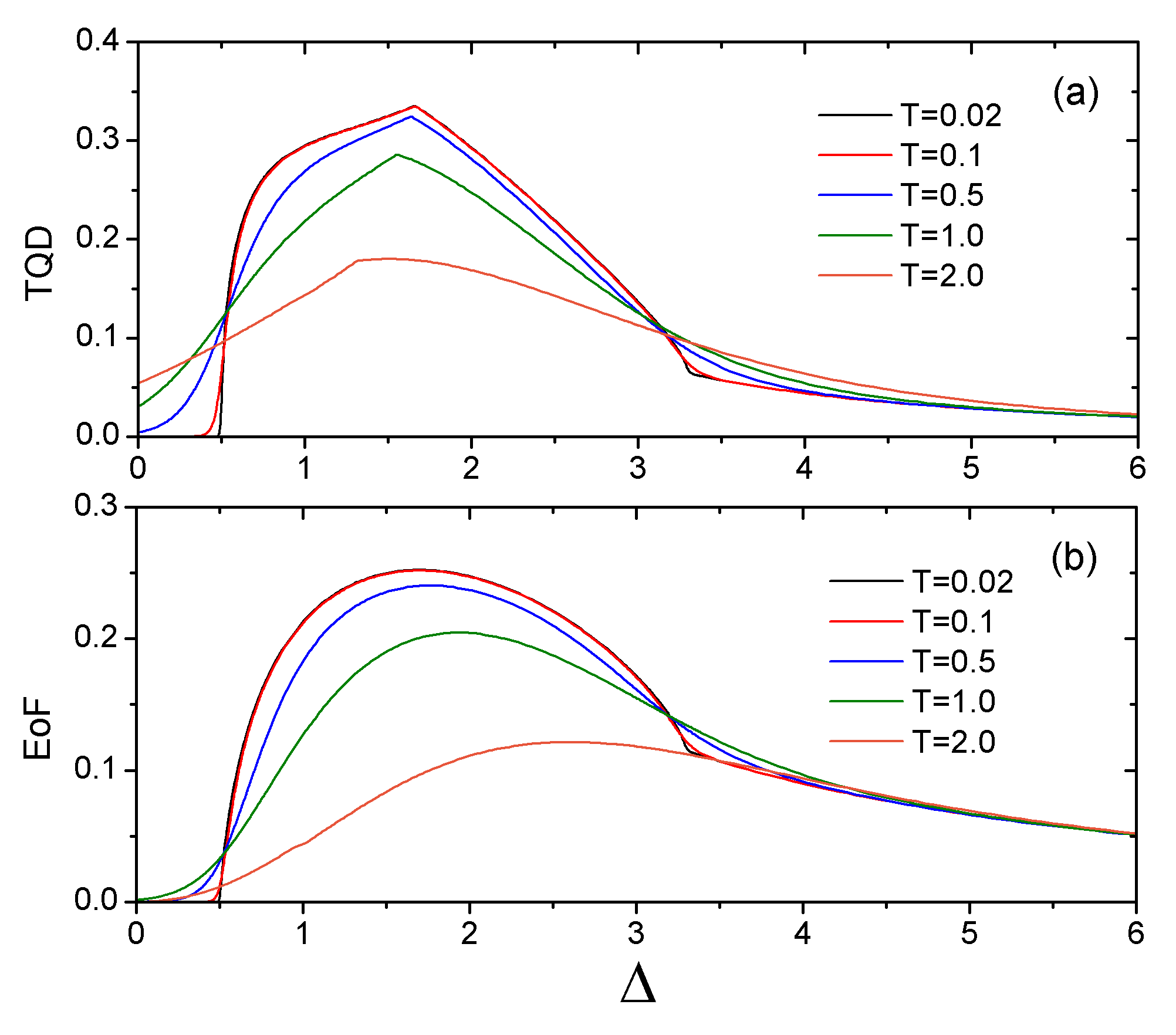
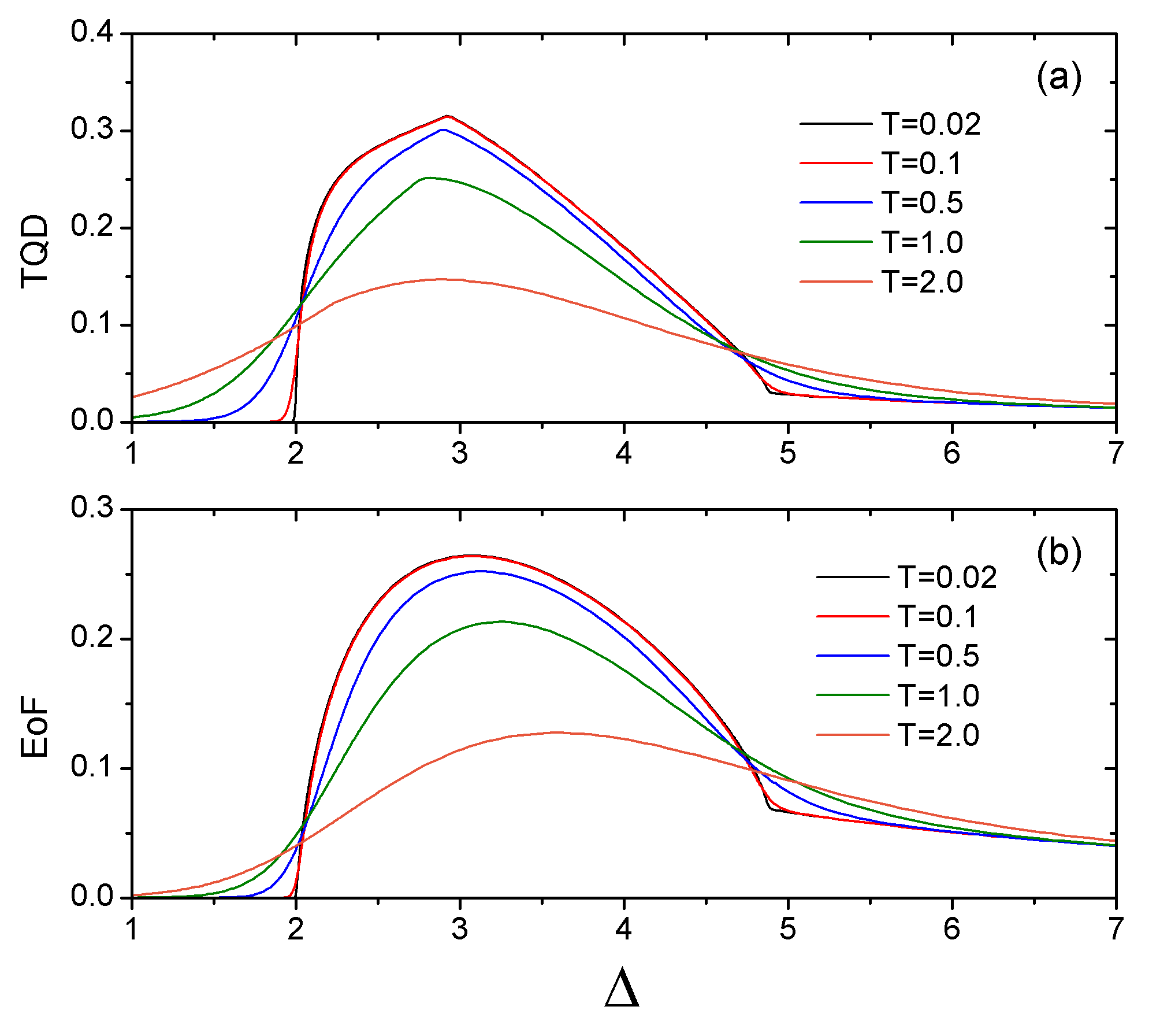
Looking at Figs. 3 and 4 we note that as the temperature increases the cusp-like behavior of TQD is smoothed while both the maximum of TQD and EoF decrease. Also, both curves of TQD and EoF become more smooth and broadened, turning these functions differentiable in the CP. Interestingly, however, if the temperature is not too high the derivatives of these quantities will still keep some features of their behavior at $T=0$. Indeed, as we have shown for $T=0$, the CP $\Delta_{1}$ is characterized by a divergence in the first derivative of both TQD and EoF while the CP $\Delta_{inf}$ by a divergence in the second derivative. As the temperature increases, though, these divergences disappear but the appropriate derivatives of TQD and EoF assume their maximum values around the CPs, a property resembling the behavior at $T=0$. To illustrate this point we plot in Fig. 5 the derivatives of TQD for $h=12$ as a function of $\Delta$ and for $kT=0.02,0.1,0.5$.

Figure 5: First-order derivative of TQD as a function of $\Delta$ for (a) $kT=0.02$, (b) $kT=0.1$, and (c) $kT=0.5$. Second-order derivative of TQD as a function of $\Delta$ for (d) $kT=0.02$, (e) $kT=0.1$ and (f) $kT=0.5$. The maximum of the first and second derivatives of TQD are very close to the CPs $\Delta_{1}=2$ and $\Delta_{inf}=4.88$, respectively. Here we fixed $h=12$. Dashed vertical bars indicate the CPs.

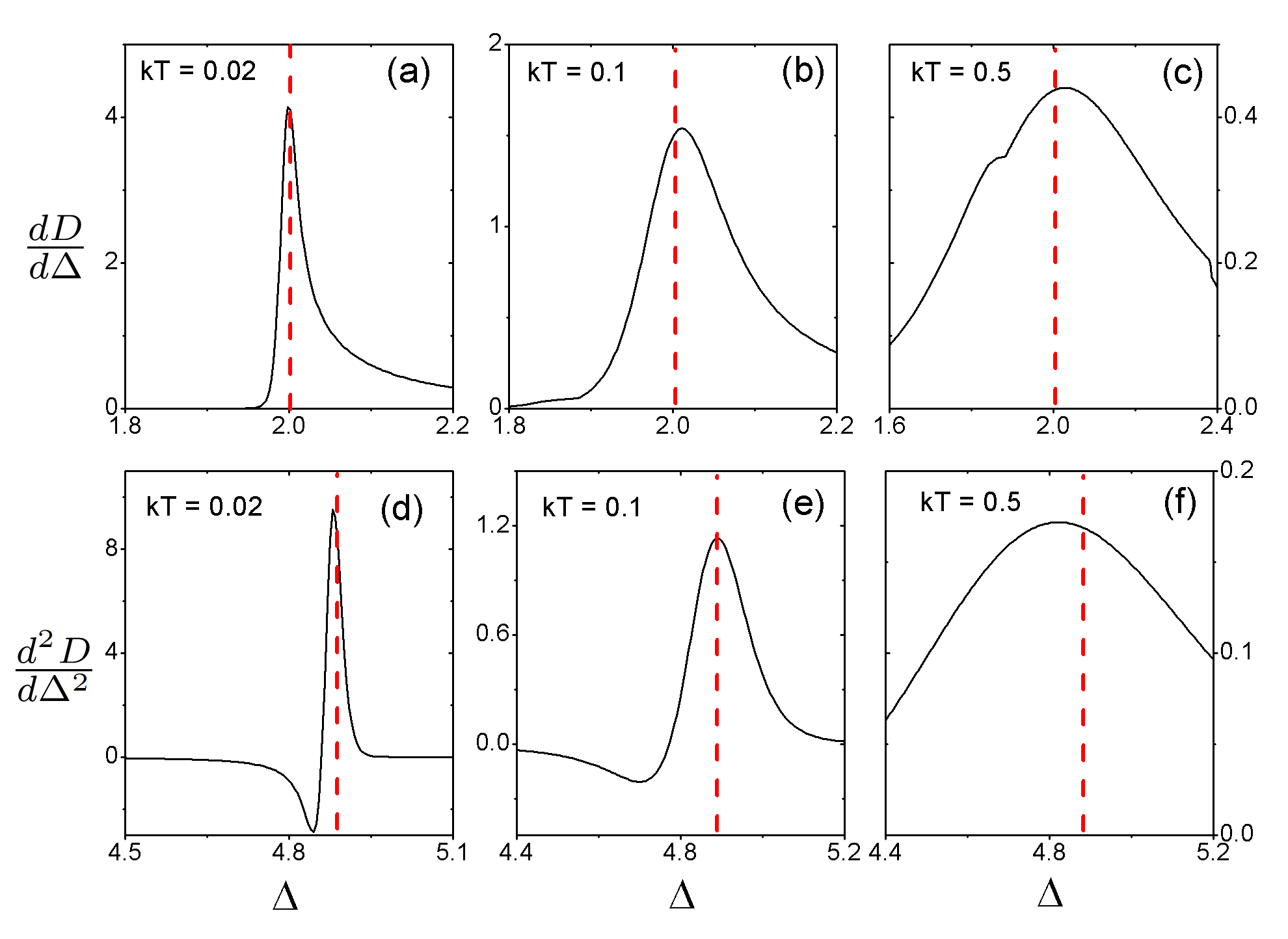
Note that the first-order derivative of TQD has a local maximum near the CP $\Delta_{1}=2$ for $kT=0.02,0.1,0.5$. The infinite-order QPT is also well characterized by a local maximum in the second-order derivative of TQD near the CP $\Delta_{inf}=4.88$ for $kT=0.02,0.1,0.5$. This procedure to determine, or at least estimate with great accuracy, the CPs with finite temperature theoretically computed data has been tested for other values of $h$ and it was proved valid. The same analysis can be applied to EoF but, as we show in the following, TQD gives better results than EoF for all sets of parameters.

In addition, in Fig. 6 we show, for several temperatures, many thermodynamic quantities for the infinite spin chain and also the pairwise correlations as a function of $\Delta$ for $h=12$.

Figure 6: (color online) Thermodynamic quantities for the XXZ model in the thermodynamic limit for $h=12$ and $kT=0.02$ (black line), $kT=0.1$ (red line), $kT=0.5$ (blue line), $kT=1.0$ (green line), and $kT=2.0$ (orange line). Here the CPs are $\Delta_{1}=2$ and $\Delta_{inf}=4.88$. For $\Delta<1$ and for the curves of the magnetization and the two-point correlations $kT$ increases from top to bottom while the opposite happens to the curves of the other quantities.

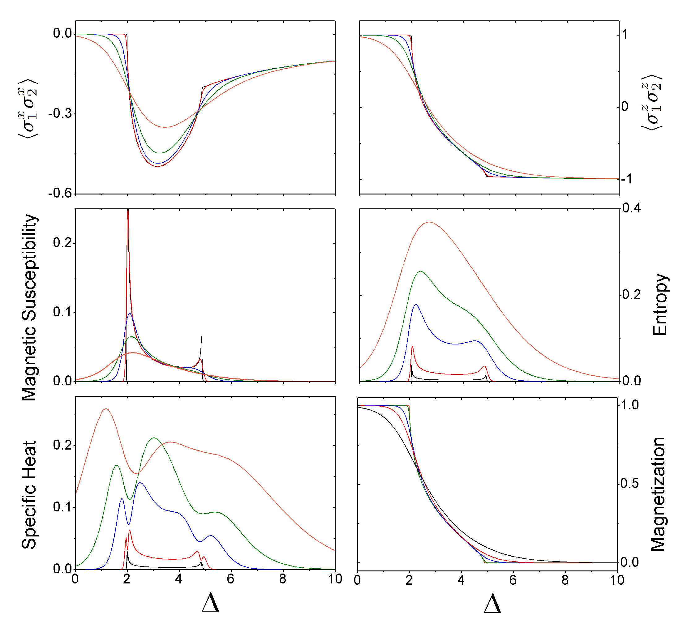
For low temperatures the CPs can be estimated by some thermodynamic quantities such as the magnetic susceptibility, entropy, and specific heat. Although TQD is not the only quantity that can determine or estimate a CP close to $T=0$ (for $h>0$) it is the best CP detector compared with other quantities tested here. This is shown in Fig. 7, where we plotted the CPs determined via TQD, EoF, and the pairwise correlations $\left\langle\sigma^{x}_{1}\sigma^{x}_{2}\right\rangle$ and $\left\langle\sigma^{z}_{1}\sigma^{z}_{2}\right\rangle$ for several temperatures. We chose to work with $h=6$ and $h=12$ but similar results are obtained for other values of the magnetic field.

Figure 7: (color online) CPs determined by TQD (square), EoF (circle), $\left\langle\sigma_{1}^{x}\sigma_{2}^{x}\right\rangle$ (up arrow), and $\left\langle\sigma_{1}^{z}\sigma_{2}^{z}\right\rangle$ (down arrow) as a function of $T$. In (a) and (b) we have $h=6$ with a first (a) and an infinite-order (b) CP; in (c) and (d) we have $h=12$ with a first (c) and an infinite-order (d) CP. Dashed horizontal lines indicate the CPs. To determine the CPs at finite $T$ we used the derivatives of TQD and EoF. As stated in the text, for some temperature ranges, the derivatives of these quantities at finite $T$ retain some information about the divergences or discontinuities that exist only at $T=0$. Note that the estimated CPs given by TQD is always closer to the exact value than the CPs coming from other quantities.

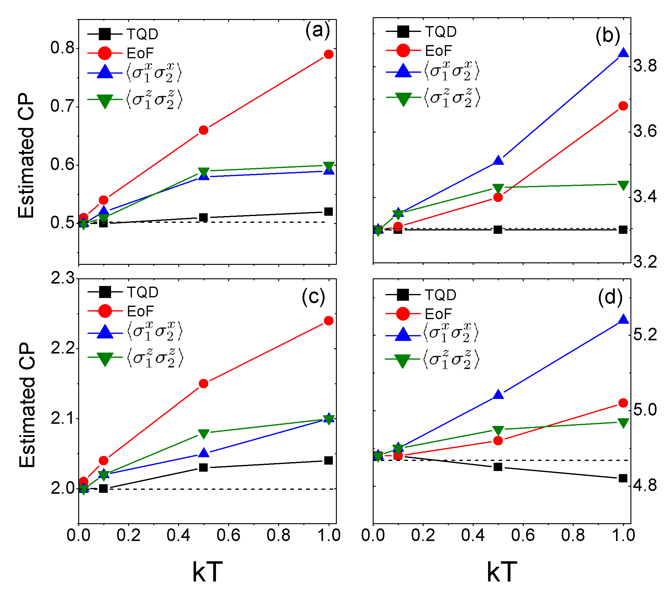
The procedure adopted to estimate the CPs when $T$ is finite comes from the behavior of TQD, EoF, and the two point correlations near or at the CPs. For example, in Figs. 2, 3, and 6 we see that in the vicinity of the CPs these quantities, as a function of $\Delta$, are either maximum or possess discontinuous/divergent first/second derivatives. Therefore, by computing the appropriate derivative and looking for its maximum/minimum we can estimate the value of the CPs even for finite $T$. Obviously, for $T=0$ these extrema are exactly at the CP. As can be seen in Fig. 7, the CPs estimated by TQD are closer to the values given in Table I than those obtained using EoF or the pairwise correlations. Indeed, from zero to $kT\approx 1.0$ the extrema of TQD is closer to the actual CP than those from the other quantities (see Fig. 7).

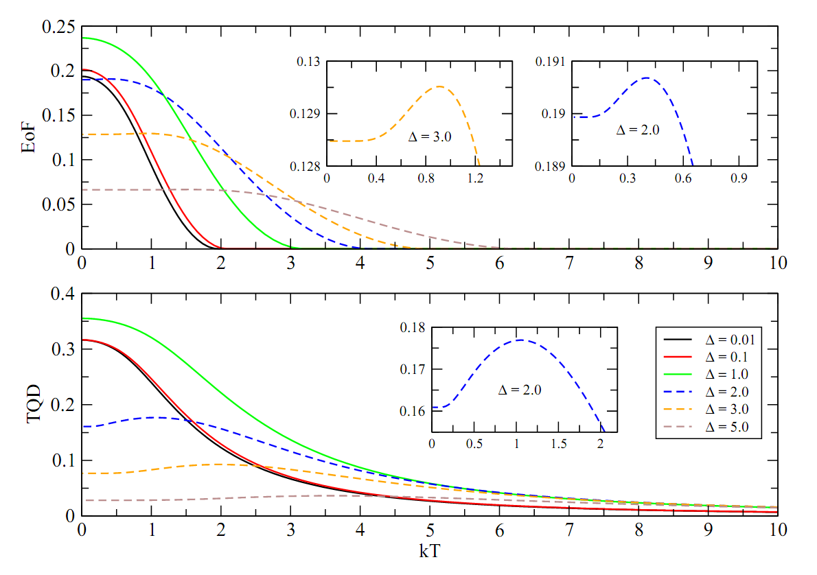
To complement our studies about the XXZ model we present in Fig. 8 the behavior of TQD and EoF as a function of temperature for $h=0$. First, we observe that EoF tends to disappear suddenly as the temperature increases while TQD is always nonzero. This sudden disappearance may be retarded by increasing the value of the anisotropy $\Delta$. The insets in Fig. 8 show a “regrowth” Wer10 of TQD and EoF with temperature. This interesting feature was already seen for the behavior of TQD of a two-spin XXZ model with no field Wer10 although the regrowth does not show up for EoF Rig04 . Therefore, the results here presented show that the regrowth of EoF with temperature, while not observed for two-spin chains without the presence of an external field Rig04 , is possible in the thermodynamic limit.

Figure 8: (color online) TQD (bottom) and EoF (top) as a function of $T$ for different values of the tuning parameter $\Delta$. The insets show the regrowth of TQD and EoF. For $\Delta\leq 1$ (solid curves) we note that as we increase $\Delta$ we also increase TQD and EoF. For $\Delta>1$ (dashed curves) this only happens for EoF at high temperatures.

III.2 The XY Model

In this section we discuss the ability of TQD and EoF to point out CPs of a QPT in the infinite one-dimensional XY model in a transverse field for finite $T$. The Hamiltonian that describes this model is given by

$$H_{xy} = -\frac{\lambda}{2}\sum_{j=1}^{L}\left[(1+\gamma)\sigma^{x}_{j}\sigma^{x}_{j+1}+(1-\gamma)\sigma^{y}_{j}\sigma^{y}_{j+1}\right]$$ (23)

$$-\sum_{j=1}^{L}\sigma^{z}_{j}.$$

The strength of the inverse of the external transverse magnetic field is represented by $\lambda$ while $\gamma$ provides the degree of anisotropy. For $\gamma=\pm 1$ we obtain the transverse Ising model while $\gamma=0$ corresponds to the XX model in a transverse field LSM , which is the $\Delta=0$ XXZ model discussed before with $J<0$. As is well-known the XY model undergoes a second-order QPT (Ising transition isingQPT ) at the CP $\lambda_{c}=1$ Dil08 , that separates a ferromagnetic ordered phase from a quantum paramagnetic phase. For $\lambda>1$ one can observe another second-order QPT at the CP $\gamma_{c}=0$ called anisotropy transition LSM ; anisQPT . Differently from the Ising transition, that is due to the action of the external field, this transition is driven by the anisotropy parameter $\gamma$ and separates a ferromagnet ordered along the $x$ direction and a ferromagnet ordered along the $y$ direction. Although both QPT have the same order they belong to different universality classes LSM ; anisQPT .

The XY Hamiltonian is $Z_{2}$-symmetric and can be exactly diagonalized LSM in the thermodynamic limit $L\rightarrow\infty$. Due to the translational invariance the two-spin density operator $\rho_{i,j}$ for spins $i$ and $j$ depends only on the distance $k=|j-i|$ between them and thus $\rho_{i,j}=\rho_{0,k}$. Therefore, the reduced density operator $\rho_{0,k}$ for the XY model at thermal equilibrium is osborne

$$\rho_{0,k} = \frac{1}{4}\left[I_{0,k}+\left\langle\sigma^{z}\right\rangle\left(\sigma^{z}_{0}+\sigma^{z}_{k}\right)\right]$$ (24)

$$+\frac{1}{4}\sum_{\alpha=x,y,z}\left\langle\sigma^{\alpha}_{0}\sigma^{\alpha}_{k}\right\rangle\sigma^{\alpha}_{0}\sigma^{\alpha}_{k},$$

where $I_{0,k}$ is the identity operator of dimension four. The transverse magnetization $\left\langle\sigma^{z}_{k}\right\rangle$ $=$ $\left\langle\sigma^{z}\right\rangle$ is

$$\left\langle\sigma^{z}\right\rangle=-\int_{0}^{\pi}(1+\lambda\cos{\phi})\tanh{(\beta\omega_{\phi})}\frac{d\phi}{2\pi\omega_{\phi}},$$ (25)

with $\omega_{\phi}=\sqrt{(\gamma\lambda\sin{\phi})^{2}+(1+\lambda\cos{\phi})^{2}}/2$. The two-point correlation functions are given by

$$\left\langle\sigma^{x}_{0}\sigma^{x}_{k}\right\rangle = \left|\begin{array}[]{cccc}G_{-1}&G_{-2}&\cdots&G_{-k}\\ G_{0}&G_{-1}&\cdots&G_{-k+1}\\ \vdots&\vdots&\ddots&\vdots\\ G_{k-2}&G_{k-3}&\cdots&G_{-1}\\ \end{array}\right|,$$ (30)

$$\left\langle\sigma^{y}_{0}\sigma^{y}_{k}\right\rangle = \left|\begin{array}[]{cccc}G_{1}&G_{0}&\cdots&G_{-k+2}\\ G_{2}&G_{1}&\cdots&G_{-k+3}\\ \vdots&\vdots&\ddots&\vdots\\ G_{k}&G_{k-1}&\cdots&G_{1}\\ \end{array}\right|,$$ (35)

$$\left\langle\sigma^{z}_{0}\sigma^{z}_{k}\right\rangle = \left\langle\sigma^{z}\right\rangle^{2}-G_{k}G_{-k},$$ (36)

where

$$G_{k} = \int_{0}^{\pi}\tanh{(\beta\omega_{\phi})}\cos{(k\phi)}(1+\lambda\cos{\phi})\frac{d\phi}{2\pi\omega_{\phi}}$$

$$- \gamma\lambda\int_{0}^{\pi}\tanh{(\beta\omega_{\phi})}\sin{(k\phi)\sin{\phi}}\frac{d\phi}{2\pi\omega_{\phi}}.$$

Using these relations and Eqs. (39) and (40) of the Appendix, EoF and TQD can be computed analytically for this model.

The ability of TQD and EoF to detect a CP for this model at $T=0$ was studied in Sar10 , where TQD and EoF from first to fourth nearest-neighbors was computed. They showed that TQD between far neighbors can still characterize a QPT while EoF is zero. This result shows an advantage of the quantum discord to the entanglement in the detection of CP. See also Ami10 for the behavior of entanglement and TQD for small $T$ in the symmetry breaking process of the XY model. Our goal here is to determine whether the quantum discord for the first and second neighbors has some advantage with respect to entanglement to spotlight a CP at finite $T$. The procedure adopted here is similar to the one employed in the analysis of the XXZ model, i.e., we compute the appropriate derivatives around the CP and look for its extremum values as indicators of QPTs.

In Figs. 9 and 10 we plot, respectively, TQD and EoF for first nearest-neighbors and second nearest-neighbors as a function of $\lambda$ for $kT=0.01,0.1,0.5$ and $\gamma=0,0.5,1.0$.

Figure 9: (color online) (a)-(c) TQD and (d)-(f) EoF as a function of $\lambda$ for $kT=0.01$ (black/solid line), $kT=0.1$ (red/dashed line) and $kT=0.5$ (blue/dotted line) for nearest-neighbors. We use three values of $\gamma$ as shown in the graphs.

Figure 10: (color online) (a)-(c) TQD and (d)-(f) EoF as a function of $\lambda$ for $kT=0.01$ (black/solid line), $kT=0.1$ (red/dashed line) and $kT=0.5$ (blue/dotted line) for second nearest-neighbors. We use three values of $\gamma$ as shown in the graphs.

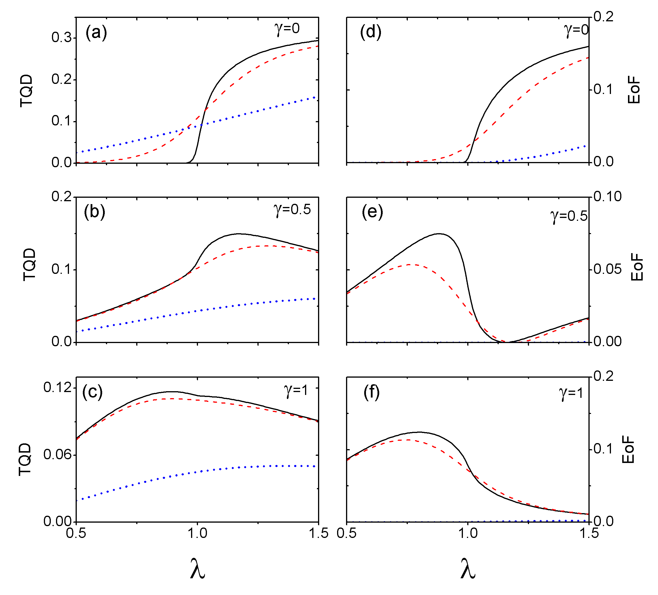
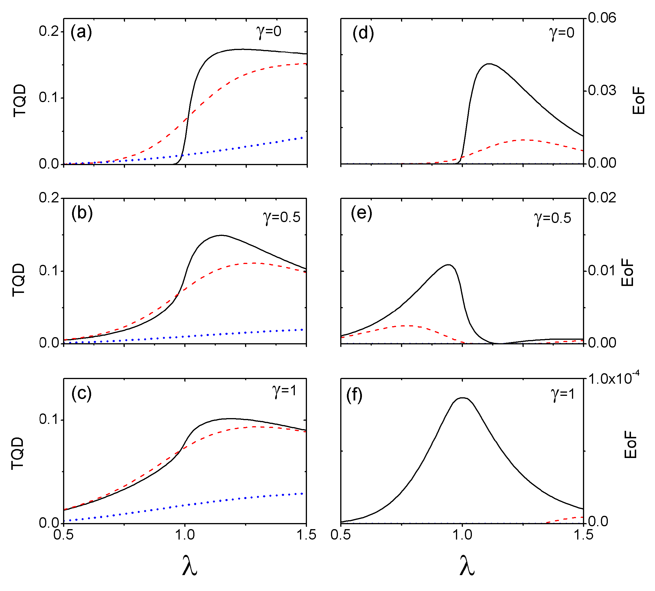
It is important to note that TQD is more resistant to thermal effects than EoF. For example, for $kT=0.5$ EoF for the first-neighbors is zero or close to zero for almost all $\lambda$ while TQD is always non-null. For second-neighbors the situation is more drastic, EoF is always zero for $kT=0.5$. The previous discussion also highlights a qualitative difference between the behavior of quantum correlations as measured by quantum discord or entanglement, especially for $\gamma=0.5$.

Since the Ising transition is a second-order QPT, the critical point at $T=0$ is characterized by a divergence or discontinuity in the first derivative of TQD or EoF Dil08 ; Sar09 ; and if the first derivative is discontinuous then the CP can also be found through the divergence of the second derivative. Similarly to the XXZ model studied in Sec. III.1, the singular behavior of TQD and EoF at the CP is attenuated as the temperature increases. However, one can still extract useful information concerning the CPs until a certain temperature. Beyond this temperature the behavior of the derivatives of TQD or EoF is not able to determine the CPs without ambiguity. With that in mind, we use the same strategy of Sec. III.1 to determine/estimate the CPs with theoretically computed data at finite $T$: if the first derivative of TQD or EoF is divergent at $T=0$ then the CP is pointed out by a local maximum or minimum at $T>0$; if the first derivative is discontinuous at $T=0$ then we look after local maximum or minimum in the second derivative for $T>0$. The results of our analysis are shown in Fig. 11 where the CPs estimated by TQD and EoF for first and second neighbors are plotted as a function of $kT$ for $\gamma=0,0.5$, and $1.0$.

Figure 11: (color online) CPs determined by TQD (black-squares) and EoF (red-circles) as a function of $kT$ for (a)-(c) first nearest-neighbors and for (d)-(f) second nearest-neighbors. Dashed horizontal lines indicate the CPs. The values of $\gamma$ used were $0$, $0.5$ and $1.0$, as shown in the graphs. The derivatives of TQD and EoF were used to estimate the CPs as explained in the text. Note that at panel (b) the curves for TQD and EoF coincide and that at panels (d) and (f) we only have two points for EoF since for greater $T$ it is zero.

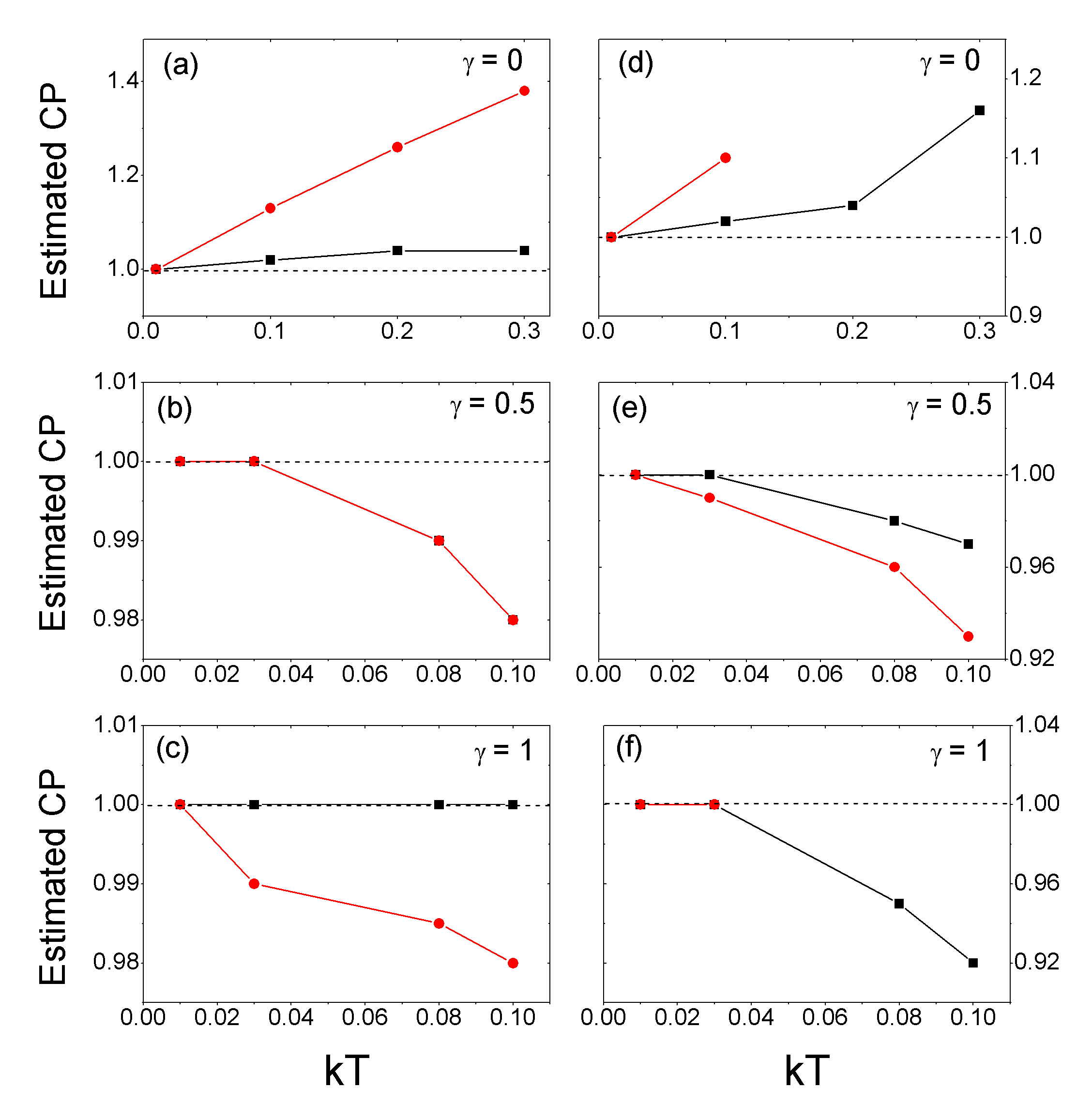
Looking at Fig. 11 we note that the CP of the Ising transition is best estimated by TQD than EoF. While for $\gamma=0.5$ and $\gamma=1$ the first-neighbor TQD is only slightly better than EoF to estimate the CP , for $\gamma=0$ the CP computed by TQD is clearly closer to $\lambda_{c}=1$ than the one estimated from EoF. Moreover, the temperature below which TQD is a good CP detector is higher for $\gamma=0$ than for $\gamma=0.5$ or $\gamma=1$ (see Fig. 11a). When we look at the second-neighbors TQD and EoF, we see that TQD is still better than EoF to estimate the CP. And in particular for $\gamma=1.0$, EoF is only useful for very tiny $T$ while TQD works relatively well for higher values of $T$. It is worth noting that for small $T$ TQD seems to approach the actual CP almost linearly as we decrease $T$. Therefore, a relatively small number of points for a couple of small temperatures allows one to correctly extrapolate to the exact value of the CP at $T=0$. This fact is also observed for the behavior of TQD in the XXZ model. An interesting future investigation, lying beyond the scope of this manuscript, would be to rigorously determine the functional form by which TQD and EoF approach the exact CP for decreasing $T$.

We close this section studying the behavior of TQD and EoF near the critical point $\gamma_{c}=0$, which is associated to the anisotropy transition that occurs only for $\lambda>1$. Hence, for definiteness, in what follows we set $\lambda=1.5$. In Fig. 12 we plot TQD and EoF for the first and second-neighbors as a function of $\gamma$ for five different values of temperature, $kT=0.001,0.1,0.5,1.0$, and $2.0$.

Figure 12: (color online) Top panels TQD and bottom panels EoF as a function of $\gamma$. From top to bottom $kT=0.001,0.1,0.5,1.0$, and $2.0$. Left panels are first nearest-neighbors and right panels second nearest-neighbors. Here we fixed $\lambda=1.5$ and the CP is $\gamma_{c}=0$ (indicated by dashed vertical lines).

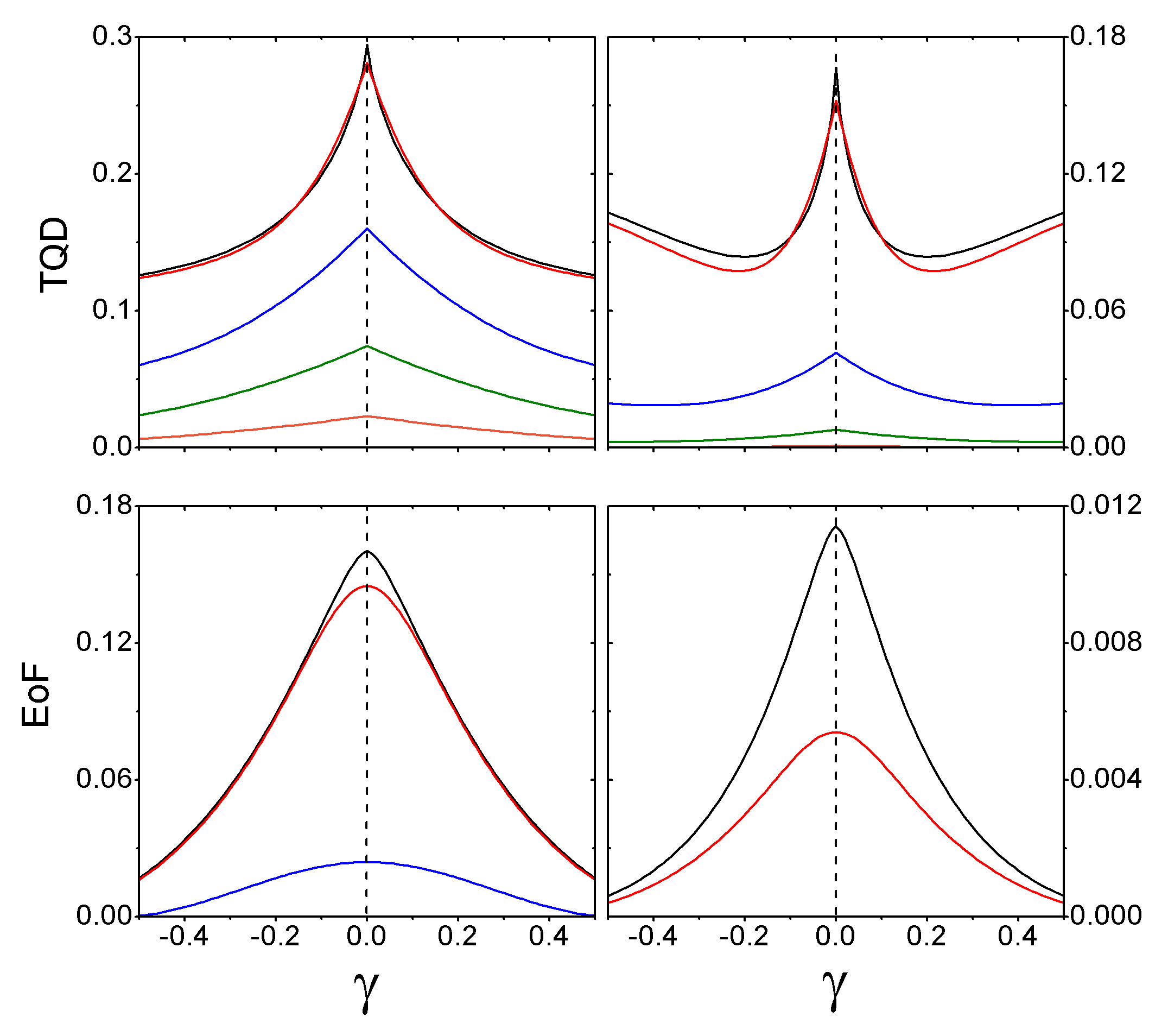
Looking at Fig. 12 we see that TQD and EoF are maximum at the CP $\gamma_{c}=0$ for first- and second-neighbors, keeping this feature as $T$ increases. However, only TQD possesses a cusp-like behavior at the CP. Furthermore, for first-neighbors TQD presents the same pattern (maximum with a cusp-like behavior) up to $kT=2.0$ while EoF vanishes for $kT\geq 1.0$. This situation is more drastic for second-neighbors: while TQD can detect the CP even for values near $kT=1.0$, EoF is nonzero only at low temperatures ($kT\lesssim 0.1$). Finally, as in the XXZ model with no external field, there is an exchange in the set of projectors that minimizes the conditional entropy (A) at the CP. This feature is characterized by a discontinuity in the first-order derivative of TQD and explains the cusp-like behavior of TQD at $\gamma_{c}=0$.

IV Conclusions

In this paper we have studied the ability of quantum correlations to spotlight critical points of quantum phase transitions when the system under investigation is away from the absolute zero, the experimentally unattainable temperature where a quantum phase transition sets in. We have mainly focused our analysis in two distinct types of quantum correlations, namely, the entanglement and the quantum discord between pairs of spins.

We first concentrated our efforts in computing those quantum correlations for an infinite chain described by the XXZ model with an external field in the $z$-direction and in equilibrium with a thermal reservoir at temperature $T$. By tracing out all but two nearest-neighbors we were able to calculate their entanglement and quantum discord for several T. For this model we also evaluated several thermodynamic quantities as well. Among all these quantities, we have shown that quantum discord is the best critical point detector at finite $T$, furnishing rather precise values for the two quantum critical points for this model, a first order and an infinite order phase transition.

We then moved to study other models, such as the infinite chain XY model and the Ising model, both of which with external transverse magnetic fields. This time we computed the entanglement and the quantum discord for first and second nearest-neighbors, assuming the system in equilibrium with a thermal reservoir at temperature $T$. For the second order phase transition usually referred to as the Ising transition, we observed that quantum discord is better suited in estimating the correct value for the quantum critical point. For the other quantum phase transition, the so called anisotropy transition (also second order), quantum discord and entanglement give excellent results for low temperatures. However, as the temperature increases quantum discord outperform entanglement as a quantum critical point estimator.

Summarizing, the previous discussions showed that for all the cases here presented, quantum discord was the best critical point estimator when one deals with finite temperature systems. Note that we never needed to know the order parameter of the phase transitions to use these quantum correlations as critical point detectors. Moreover, we have also showed that using the quantum discord (our best critical point estimator), and with theoretically computed data for several $T$, we can with reasonable accuracy infer the actual value of the critical point at $T=0$ by looking at the behavior of these quantities when $T$ approaches zero. Therefore, we have given strong indications that entanglement and in special quantum discord are useful quantities in estimating quantum critical points when the available data are away from the absolute zero. This fact alone shows that these quantities are an important tool in the study of quantum phase transitions in realistic experimental scenarios, where one is always working at finite $T$ and has perhaps no clue of the order parameter of the phase transition taking place.

*

Appendix A Closed expressions for QD and EoF

In Sec. III, after tracing out all spins but two in an infinite chain, the two-qubit reduced density matrix is of X-form,

$$\rho_{AB}=\left(\begin{array}[]{cccc}\rho_{11}&0&0&\rho_{14}\\ 0&\rho_{22}&\rho_{23}&0\\ 0&\rho_{23}&\rho_{22}&0\\ \rho_{14}&0&0&\rho_{44}\end{array}\right).$$ (37)

It is easy to see that for this density matrix $\mathcal{S}(A)=\mathcal{S}(B)=-\sum_{i=1}^{2}\beta_{i}\log_{2}\beta_{i}$, with $\beta_{1}=\rho_{11}+\rho_{22}$ and $\beta_{2}=\rho_{44}+\rho_{22}$, implying that QD is a symmetric quantity. For the density operator (37) this minimization can be done analytically, as previously demonstrated in discordX , resulting in the following expression,

$$\mathcal{S}_{q}(A|B)\!=\!\min\!\left\{\beta_{1}\mathcal{F}(\theta_{1})+\beta_{2}\mathcal{F}(\theta_{2}),\mathcal{F}(\theta_{3}),\mathcal{F}(\theta_{4})\right\},$$

where $\mathcal{F}(\theta)=-\frac{1-\theta}{2}\log_{2}\frac{1-\theta}{2}-\frac{1+\theta}{2}\log_{2}\frac{1+\theta}{2}$ and

$$\theta_{1} = \frac{1}{\beta_{1}}\left|\rho_{22}-\rho_{11}\right|,$$

$$\theta_{2} = \frac{1}{\beta_{2}}\left|\rho_{22}-\rho_{44}\right|,$$

$$\theta_{3} = \sqrt{4(\rho_{14}-\rho_{23})^{2}+(\rho_{11}-\rho_{44})^{2}},$$

$$\theta_{4} = \sqrt{4(\rho_{14}+\rho_{23})^{2}+(\rho_{11}-\rho_{44})^{2}}.$$

Using (A) in Eq. (3) and calculating the joint entropy $\mathcal{S}(A,B)$ of the density operator (37), the quantum discord is obtained as

$$D\left(\rho_{AB}\right) = -\sum_{i=1}^{2}\beta_{i}\log_{2}\beta_{i}+\sum_{j=1}^{4}\lambda_{j}\log_{2}\lambda_{j}$$ (39)

$$+\mathcal{S}_{q}(A|B),$$

where $\lambda_{j}$ are the eigenvalues of (37),

$$\lambda_{1} = \frac{1}{2}\left[\rho_{11}+\rho_{44}+\sqrt{(\rho_{11}-\rho_{44})^{2}+4\left|\rho_{14}\right|^{2}}\right],$$

$$\lambda_{2} = \frac{1}{2}\left[\rho_{11}+\rho_{44}-\sqrt{(\rho_{11}-\rho_{44})^{2}+4\left|\rho_{14}\right|^{2}}\right],$$

$$\lambda_{3} = \rho_{22}+\left|\rho_{23}\right|,$$

$$\lambda_{4} = \rho_{22}-\left|\rho_{23}\right|.$$

When $\rho_{14}\rho_{23}\neq 0$ Eq. (A) provides the correct value for the quantum conditional entropy. However, for $\rho_{14}\rho_{23}=0$ the correct value of the conditional entropy is not always given by this expression numDIS ; valAE . In the latter case the minimization depends on only one single parameter and should be numerically carried out. For all the cases studied here, however, the numerical calculations agreed with the analytical expression of quantum discord.

Finally, for the density operator (37) the EoF is given by Woo98

$$EoF(\rho_{AB}) = -g\log_{2}g-(1-g)\log_{2}(1-g),$$ (40)

where $g=(1+\sqrt{1-C^{2}})/2$ and $C=2\max\left\{0,\Lambda_{1},\Lambda_{2}\right\}$ is the concurrence with $\Lambda_{1}=|\rho_{14}|-\sqrt{\rho_{22}\rho_{33}}$ and $\Lambda_{2}=|\rho_{23}|-\sqrt{\rho_{11}\rho_{44}}$.

References

- (1) S. Sachdev, Quantum Phase Transitions (Cambridge University Press, Cambridge, 1999).
- (2) S. Rowley, R. Smith, M. Dean, L. Spalek, M. Sutherland, M. Saxena, P. Alireza, C. Ko, C. Liu, E. Pugh, S. Sebastian, and G. Lonzarich, Phys. Status Solidi B 247, 469 (2010).
- (3) V. F. Gantmakher and V. T. Dolgopolov, Physics-Uspekhi 53, 1 (2010).
- (4) M. Greiner, O. Mandel, T. Esslinger, T.W. Hänsch, and I. Bloch, Nature (London) 415, 39 (2002).
- (5) L.-A. Wu, M. S. Sarandy, and D. A. Lidar, Phys. Rev. Lett. 93, 250404 (2004).
- (6) T. R. de Oliveira, G. Rigolin, M. C. de Oliveira, and E. Miranda, Phys. Rev. Lett. 97, 170401 (2006); T. R. de Oliveira, G. Rigolin, and M. C. de Oliveira, Phys. Rev. A 73, 010305(R) (2006); G. Rigolin, T. R. de Oliveira, and M. C. de Oliveira, Phys. Rev. A 74, 022314 (2006); T. R. de Oliveira, G. Rigolin, M. C. de Oliveira, and E. Miranda, Phys. Rev. A 77, 032325 (2008).
- (7) H. Barnum, E. Knill, G. Ortiz, R. Somma, and L. Viola, Phys. Rev. Lett. 92, 107902 (2004); R. Somma, G. Ortiz, H. Barnum, E. Knill, and L. Viola, Phys. Rev. A 70, 042311 (2004).
- (8) H. Ollivier and W. H. Zurek, Phys. Rev. Lett. 88, 017901 (2001);
- (9) L. Henderson and V. Vedral, J. Phys. A 34, 6899 (2001).
- (10) R. Dillenschneider, Phys. Rev. B 78, 224413 (2008).
- (11) M. S. Sarandy, Phys. Rev. A 80, 022108 (2009).
- (12) T. Werlang, C. Trippe, G.A.P. Ribeiro, and G. Rigolin, Phys. Rev. Lett. 105, 095702 (2010).
- (13) M. A. Nielsen and I. L. Chuang, Quantum Computation and Quantum Information (Cambridge University Press, Cambridge, 2000).
- (14) T. M. Cover and J. A. Thomas, Elements of Information Theory (Wiley-Interscience, New York, 2006).
- (15) A. Peres, Quantum Theory: Concepts and Methods (Kluwer Academic Publishers, New York, 2002).
- (16) B. Dakic, V. Vedral, and C. Brukner, Phys. Rev. Lett. 105, 190502 (2010).
- (17) Similarly, we have if and only if there exists a von Neumann measurement such that .
- (18) J. Oppenheim, M. Horodecki, P. Horodecki, and R. Horodecki, Phys. Rev. Lett. 89, 180402 (2002); K. Modi, T. Paterek, W. Son, V. Vedral, and M. Williamson, Phys. Rev. Lett. 104, 080501 (2010).
- (19) M. C. Arnesen, S. Bose, and V. Vedral, Phys. Rev. Lett. 87, 017901 (2001).
- (20) T. Werlang and G. Rigolin, Phys. Rev. A 81, 044101 (2010).
- (21) S. Hamieh, R. Kobes, and H. Zaraket, Phys. Rev. A 70, 052325 (2004).
- (22) D. Girolami and G. Adesso, eprint arXiv:1103.3189v1 [quant-ph].
- (23) R. F. Werner, Phys. Rev. A 40, 4277 (1989).
- (24) A. Peres, Phys. Rev. Lett. 77, 1413 (1996).
- (25) W. K. Wootters, Phys. Rev. Lett. 80, 2245 (1998); T. Yu and J. H. Eberly, Quantum Inf. Comp. 7,459 (2007).
- (26) M. Ali, A. R. P. Rau, and G. Alber, Phys. Rev. A 81, 042105 (2010); ibid. 82, 069902(E) (2010).
- (27) C.N. Yang and C.P. Yang, Phys. Rev. 147, 303 (1966).
- (28) A. Klümper, Ann. Phys. 1, 540 (1992); A. Klümper, Z. Phys. B 91, 507 (1993).
- (29) M. Bortz and F. Göhmann, Eur. Phys. J. B 46, 399 (2005); H.E. Boos, J. Damerau, F. Göhmann, A. Klümper, J. Suzuki, and A. Weiße, J. Stat. Mech. (2008) P08010; C. Trippe, F. Göhmann, and A. Klümper, Eur. Phys. J. B 73, 253 (2010).
- (30) M. Takahashi, Thermodynamics of one-dimensional solvable models (Cambridge University Press, Cambridge, England, 1999).
- (31) J. Cloizeaux and M. Gaudin, J. Math. Phys. 7, 1384 (1966).
- (32) C. C. Rulli and M. S. Sarandy, Phys. Rev. A 81, 032334 (2010).
- (33) J. Maziero, L. C. Céleri, R. M. Serra, and V. Vedral, Phys. Rev. A 80, 044102 (2009).
- (34) G. Rigolin, Int. J. Quantum Inform. 2, 393 (2004).
- (35) E. Lieb, T. Schultz, and D. Mattis, Ann. Phys. 16, 407 (1961); E. Barouch, B.M. McCoy, and M. Dresden, Phys. Rev. A 2, 1075 (1970); E. Barouch and B.M. McCoy, Phys. Rev. A 3, 786 (1971).
- (36) P. Pfeuty, Ann. Phys. (New York) 57, 79 (1970).
- (37) M. Zhong and P. Tong, J. Phys. A: Math. Theor. 43, 505302 (2010).
- (38) T. J. Osborne and M. A. Nielsen, Phys. Rev. A 66, 032110 (2002).
- (39) J. Maziero, H. C. Guzman, L. C. Céleri, M. S. Sarandy, and R. M. Serra, Phys. Rev. A 82, 012106 (2010).
- (40) B. Tomasello, D. Rossini, A. Hamma, and L. Amico, eprint arXiv:1012.4270v1 [quant-ph].
- (41) Q. Chen, C. Zhang, S. Yu, X.X. Yi, and C. H. Oh, eprint arXiv:1102.0181v1 [quant-ph].