Construction of modulated amplitude waves via averaging in collisionally inhomogeneous Bose-Einstein condensates

Abstract

We apply the averaging method to analyze spatio-temportal structures in nonlinear Schrödinger equations and thereby study the dynamics of quasi-one-dimensional collisionally inhomogeneous Bose-Einstein condensates with the scattering length varying periodically in spatial and crossing zero. Infinitely many (positive measure set) modulated amplitude waves (periodic and quasi-periodic), which are instable, can be proved to exist by adjusting the integration constant $c$ on some open interval. Finally, some numerical simulations support our results.

1 Introduction

Since the experimental realization of Bose-Einstein condensates (BECs) in the mid-1990s [1, 2], the study of matter-wave patterns including existence and stability in BECs has drawn a great deal of interest from experimentalists [3, 4] and theorists [5, 6, 7, 8].

In atomic physics, the Feshbach resonance of the scattering length of interatomic interactions is used for control of Bose-Einstein condensates [9, 10]. We consider the main model of this paper for Feshbach resonance given by the perturbed Gross-Pitaevskii (GP) equation of the dimensionless form [11]

$$i\frac{\partial\psi}{\partial t}=-\frac{1}{2}\frac{\partial^{2}\psi}{\partial x^{2}}+\tilde{g}(x)|\psi|^{2}\psi+\tilde{V}(x)\psi,$$ (1.1)

where the nonlinearity coefficient $\tilde{g}(x)$ varies in space. In Eq. (1.1), $\psi$ is the mean-field condensate wave function (with density $|\psi|^{2}$ measured in units of the peak 1D density $n_{0}$), $x$ and $t$ are normalized, respectively, to the healing length $\xi=\hbar/\sqrt{n_{0}|g_{1}|m}$ and $\xi/c$ (where $c=\hbar\sqrt{n_{0}|g_{1}|/m}$ is the Bogoliubov speed of sound), and energy is measured in units of the chemical potential $\delta=g_{1}n_{0}$. In the above expressions, $g_{1}=2\hbar\omega_{\perp}a_{0}$, where $\omega_{\perp}$ denotes the confining frequency in the transverse direction, and $a_{0}$ is a characteristic (constant) value of the scattering length relatively close to the Feshbach resonance. Finally, $\tilde{V}(x)$ is the rescaled external trapping potential, and the $x$-dependent nonlinearity is given by $\tilde{g}(x)=a(x)/a_{0}$, where $a(x)$ is the spatially varying scattering length.

In the past few years, GP equation (1.1) has been widely studied, such as the stability and dynamics of bright, dark solitary waves [12, 13, 14, 15] and modulated amplitude waves (MAWs) [11].

In order to study the dynamics of BECs with scattering length subjected to a spatially periodic variation, Porter and Kevrekidis et al. [11] transform equation (1.1) into a new GP equation with a constant coefficient and an additional effective potential

$$i\frac{\partial\psi}{\partial t} =-\frac{1}{2}\frac{\partial^{2}\psi}{\partial x^{2}}+|\psi|^{2}\psi+\tilde{V}(x)\psi+\tilde{V}_{eff}(x)\psi,$$

$$\tilde{V}_{eff}(x) =\frac{1}{2}\frac{f^{\prime\prime}}{f}-\frac{(f^{\prime})^{2}}{f^{2}}+\frac{f^{\prime}}{f}\frac{\partial}{\partial x}$$

with $f(x)=\sqrt{\tilde{g}(x)}$, then the transformed equation was investigated. For weak underlying inhomogeneity, the effective potential takes a form resembling a superlattice, and the amplitude dynamics of the solutions of the constant-coefficient GP equation obey a nonlinear generalization of the Ince equation. In the small-amplitude limit, they use averaging to construct analytical solutions for modulated amplitude waves (MAWs), whose stability was subsequently examined using both numerical simulations of the original GP equation and fixed-point computations with the MAWs as numerically exact solutions. However, mentioned in their paper, the transformation $\tilde{\psi}=\sqrt{\tilde{g}(x)}\psi$ applies only in the case when $\tilde{g}(x)$ does not cross zero. A natural question is that for general periodic function $\tilde{g}(x)$, whether the similar results upon the dynamics can be obtained. On the other hand, the phases of MAWs considered in [11] are trivial, which are corresponding to standing waves. Thus, another question is that whether the MAWs with nontrivial phases can exist.

With these questions discussed above, in this paper we investigate the existence and stability of MAWs with nontrivial phases in collisionally inhomogeneous BECs modeled by GP equation (1.1) for general small periodic function $\tilde{g}(x)$. The method is based on averaging, and we use the averaging principle to replace a GP equation by the corresponding averaged system. Along this paper, we assume that $g(x)$ and $V(x)$ are analytic and periodic functions with the least positive period $T=\pi/\sqrt{\delta}$.

The rest paper is organized as follows. In Section 2, we introduce modulated amplitude waves involving periodic and quasi-periodic, and an averaging theorem is obtained in Section 3. In Section 4 we investigate the existence and stability of equilibrium points for the averaged system and thereby study the periodic orbits and a numerical simulation is presented as prescribed parameters in Section 5. Finally, we summarize our results in Section 6.

2 Coherent structure

we consider uniformly propagating coherent structures with the ansatz

$$\psi(t,x)=R(x)\exp(i[\Theta(x)-\mu t]),$$ (2.1)

where $R(x)\in\mathbb{R}$ gives the amplitude dynamics of the condensate wave function, $\theta(x)$ determines the phase dynamics, and the “chemical potential” $\mu$, defined as the energy it takes to add one more particle to the system, is proportional to the number of atoms trapped in the condensate. When the (temporally periodic) coherent structure (2.1) is also spatially periodic, it is called a modulated amplitude wave (MAW) [16, 17]. Similarly, a solution of the equation (1.1) with the (temporally periodic) coherent structure (2.1) is called a quasi-periodic modulated amplitude wave (QMAW) if it is also spatially quasi-periodic.

Inserting (2.1) into (1.1), we obtain the following two couple nonlinear ordinary differential equations

$$R^{\prime\prime}+\delta R-\frac{c^{2}}{R^{3}}+\varepsilon g(x)R^{3}+\varepsilon V(x)R=0,$$ (2.2)

$$\Theta^{\prime\prime}+2\Theta^{\prime}R^{\prime}/R=0~{}\Rightarrow~{}\Theta^{\prime}(x)=\frac{c}{R^{2}},\quad\quad$$ (2.3)

where

$$\varepsilon g(x):=-\tilde{g}(x),~{}\varepsilon V(x):=-\tilde{V}(x)$$

and the integration constant $c$, determined by the velocity and number density, plays the role of “angular momentum” [18].

In case of $c=0$, the phase of the condensate wave function (standing wave) is trivial and constant. In the general case, $c\neq 0$, the system (2.2) becomes more complicated and the phase is no longer constant [19]. Even the amplitude $R(x)$, a solution of (2.2), is $T$-periodic, the corresponding condensate wave function $\psi(x,t)$ may be not periodic, but quasi-periodic, with respect to the spatial variable $x$ [20].

3 Averaging theorem

Rewrite equation (2.2) in the planar equivalent form

$$\left\{\begin{array}[]{ll}R^{\prime}=S\\ S^{\prime}=-\delta R+\displaystyle\frac{c^{2}}{R^{3}}-\varepsilon g(x)R^{3}-\varepsilon V(x)R.\end{array}\right.$$ (3.1)

Generally, averaging method involves two steps: transforming to standard form; solving the averaging equation. In order to proceed we need to transform (3.1) to a standard form for the method of averaging.

Lemma 3.1.

Under the transformation $\Psi:\mathbb{T}\times\big{(}\sqrt[4]{\frac{c^{2}}{\delta}},+\infty\big{)}\rightarrow(0,+\infty)\times\mathbb{R}$ defined by

$$\left\{\begin{array}[]{ll}R=\rho\sqrt{\cos^{2}(\sqrt{\delta}x+\theta)+\displaystyle\frac{c^{2}}{\delta\rho^{4}}\sin^{2}(\sqrt{\delta}x+\theta)}\\[20.00003pt] S=\rho\sqrt{\delta}\left(\displaystyle\frac{c^{2}}{\delta\rho^{4}}-1\right)\displaystyle\frac{\cos(\sqrt{\delta}x+\theta)\sin(\sqrt{\delta}x+\theta)}{\sqrt{\cos^{2}(\sqrt{\delta}x+\theta)+\displaystyle\frac{c^{2}}{\delta\rho^{4}}\sin^{2}(\sqrt{\delta}x+\theta)}},\end{array}\right.$$

system (3.1) changes into a new system

$$\left\{\begin{array}[]{llll}\rho^{\prime}=\varepsilon\left\{\displaystyle\frac{g(x)}{\sqrt{\delta}}\rho^{3}\left[\frac{1}{4}(1+\frac{c^{2}}{\delta\rho^{4}})\sin 2(\sqrt{\delta}x+\theta)+\frac{1}{8}(1-\frac{c^{2}}{\delta\rho^{4}})\sin 4(\sqrt{\delta}x+\theta)\right]\right.\\ ~{}~{}~{}~{}~{}~{}~{}~{}~{}~{}~{}~{}~{}~{}~{}~{}~{}~{}~{}~{}~{}~{}~{}~{}~{}~{}~{}~{}~{}~{}~{}~{}~{}~{}~{}~{}~{}+\left.\displaystyle\frac{\rho}{2\sqrt{\delta}}V(x)\sin 2(\sqrt{\delta}x+\theta)\right\}\\[20.00003pt] \theta^{\prime}=\varepsilon\left\{\displaystyle\frac{g(x)(\delta\rho^{4}+c^{2})}{8\delta^{2}\rho^{2}}\big{(}3+\cos 4(\sqrt{\delta}x+\theta)\big{)}+\displaystyle\frac{g(x)(\delta^{2}\rho^{8}+c^{4})}{2\delta^{2}\rho^{2}(\delta\rho^{4}-c^{2})}\cos 2(\sqrt{\delta}x+\theta)\right.\\[10.00002pt] ~{}~{}~{}~{}~{}~{}~{}~{}~{}~{}~{}~{}~{}~{}~{}~{}~{}~{}~{}~{}~{}~{}~{}~{}~{}~{}~{}~{}~{}~{}~{}~{}~{}~{}~{}~{}~{}+\left.\displaystyle\frac{1}{2\delta}V(x)\left(1+\frac{\delta\rho^{4}+c^{2}}{\delta\rho^{4}-c^{2}}\cos 2(\sqrt{\delta}x+\theta)\right)\right\}\end{array}\right.$$ (3.2)

with the new coordinates $(\theta,\rho)$ in the half-plane $\mathbb{T}\times\big{(}\sqrt[4]{\frac{c^{2}}{\delta}},+\infty\big{)}$.

The transformation $\Psi$ arises from the variation of constant by using the solutions of the unperturbed system ($\varepsilon=0$), and $\rho$ plays the role of “energy”. When taking the integration constant $c=0$, the transformation $\Psi$ is the usual change of polar coordinates in the half plane. The proof the Lemma 3.1 follows from the basic computation (maybe lengthy), and it can be found in [20].

Now write the $T$-periodic functions $g(x),V(x)$ as the Fourier series

$$g(x) =g_{0}+\sum_{k=1}^{\infty}(\alpha_{k}\sin 2k\sqrt{\delta}x+\beta_{k}\cos 2k\sqrt{\delta}x),$$ (3.3)

$$V(x) =v_{0}+\sum_{k=1}^{\infty}(a_{k}\sin 2k\sqrt{\delta}x+b_{k}\cos 2k\sqrt{\delta}x).$$ (3.4)

After inserting (3.3) and (3.4) into (3.2) and then multiplying the right side of (3.2) by $1/T$ and integrating from $0$ to $T$, we obtain the averaged system

$$\left\{\begin{array}[]{llll}\rho^{\prime}=\varepsilon\left\{\displaystyle\frac{\delta\bar{\rho}^{4}+c^{2}}{8\delta\sqrt{\delta}\bar{\rho}}A\sin(2\bar{\theta}+\phi_{1})+\displaystyle\frac{\bar{\rho}}{4\sqrt{\delta}}B\sin(2\bar{\theta}+\phi_{2})\right\}:=\varepsilon F_{1}(\bar{\theta},\bar{\rho})\\[20.00003pt] \theta^{\prime}=\varepsilon\left\{\displaystyle\frac{3g_{0}(\delta\bar{\rho}^{4}+c^{2})}{8\delta^{2}\bar{\rho}^{2}}+\displaystyle\frac{(\delta^{2}\bar{\rho}^{8}+c^{4})}{4\delta^{2}\bar{\rho}^{2}(\delta\bar{\rho}^{4}-c^{2})}A\cos(2\bar{\theta}+\phi_{1})\right.\\[10.00002pt] ~{}~{}~{}~{}~{}~{}~{}~{}~{}~{}~{}~{}~{}~{}~{}~{}~{}~{}~{}~{}~{}~{}~{}~{}~{}+\left.\displaystyle\frac{v_{0}}{2\delta}+\displaystyle\frac{1}{4\delta}\frac{\delta\bar{\rho}^{4}+c^{2}}{\delta\bar{\rho}^{4}-c^{2}}B\cos(2\bar{\theta}+\phi_{2})\right\}:=\varepsilon F_{2}(\bar{\theta},\bar{\rho}),\end{array}\right.$$ (3.5)

where

$$A =\sqrt{\alpha_{1}^{2}+\beta_{1}^{2}},~{}~{}~{}B=\sqrt{a_{1}^{2}+b_{1}^{2}},$$

$$\phi_{1} =\arctan\frac{\alpha_{1}}{\beta_{1}},~{}(\phi_{1}=\frac{\pi}{2}\cdot\mathrm{sign}(\phi_{1}),~{}\text{if}~{}\beta_{1}=0),$$

$$\phi_{1} =\arctan\frac{a_{1}}{b_{1}},~{}(\phi_{1}=\frac{\pi}{2}\cdot\mathrm{sign}(a_{1}),~{}\text{if}~{}b_{1}=0).$$

Theorem 3.1.

[ Averaging theorem ] There exists a $c^{r},r\geq 2$, change of variables

$$\rho=\bar{\rho}+\varepsilon w_{1}(\bar{\theta},\bar{\rho},x,\varepsilon),~{}~{}\theta=\bar{\theta}+\varepsilon w_{2}(\bar{\theta},\bar{\rho},x,\varepsilon)$$

with $w_{1},w_{2}$ $T$-periodic functions of $x$, transforming (3.2) into

$$\left\{\begin{array}[]{ll}\bar{\rho}^{\prime}=\varepsilon F_{1}(\bar{\theta},\bar{\rho})+\varepsilon^{2}g_{1}(\bar{\theta},\bar{\rho},x,\varepsilon)\\[5.0pt] \bar{\theta}^{\prime}=\varepsilon F_{2}(\bar{\theta},\bar{\rho})+\varepsilon^{2}g_{2}(\bar{\theta},\bar{\rho},x,\varepsilon)\end{array}\right.$$ (3.6)

with $g_{1},g_{2}$ $T$-periodic functions of $x$. Moreover,

(i) If $(\theta_{\varepsilon}(x),\rho_{\varepsilon}(x))$ and $(\bar{\theta}(x),\bar{\rho}(x))$ are solutions of the original system (3.2) and averaged system (3.5) respectively, with the initial value such that

$$|\,\rho_{\varepsilon}(0)-\bar{\rho}(0)|+|\,\theta_{\varepsilon}(0)-\bar{\theta}(0)|=\mathcal{O}(\varepsilon),$$

then

$$|\,\rho_{\varepsilon}(x)-\rho_{0}(x)|+|\,\theta_{\varepsilon}(x)-\theta_{0}(x)|=\mathcal{O}(\varepsilon),$$

for times $x$ of order $1/\varepsilon$.

(ii) If $P_{0}$ is an equilibrium point of (3.5) such that the corresponding Jacobian matrix has no eigenvalue equal to zero, then (3.2) admits a $T$-periodic solution $(\theta_{\varepsilon}(t),\rho_{\varepsilon}(t))$ such that $|(\rho_{\varepsilon}(t),\theta_{\varepsilon}(t))-P_{0}|=\mathcal{O}(\varepsilon),$ for sufficiently small $\varepsilon$; if $P_{0}$ is a hyperbolic equilibrium point of (3.5), then there exists $\epsilon_{0}>0$ such that, for all $0<\varepsilon<\varepsilon_{0}$, system (3.2) possesses a hyperbolic periodic orbits $\gamma_{\varepsilon}(x)=P_{0}+\mathcal{O}(\varepsilon)$ of the same stability type as $P_{0}$.

(iii) If $(\theta_{\varepsilon}(x),\rho_{\varepsilon}(x))\in W^{s}(\gamma_{\varepsilon}(x))$ is a solution of system (3.2) lying in the stable manifold of the hyperbolic periodic orbit $\gamma_{\varepsilon}(x)=P_{0}+\mathcal{O}(\varepsilon)$, $(\bar{\theta}(x),\bar{\rho}(x))\in W^{s}(P_{0})$ is a solution of system (3.5) lying in the stable manifold of the hyperbolic equilibrium point $P_{0}$ and

$$|(\theta_{\varepsilon}(0)),\rho_{\varepsilon}(0)-(\bar{\theta}(0),\bar{\rho}(0))|=\mathcal{O}(\varepsilon),$$

then

$$|(\theta_{\varepsilon}(x),\rho_{\varepsilon}(x))-(\bar{\theta}(x),\bar{\rho}(x))|=\mathcal{O}(\varepsilon),$$

for $x\in[0,+\infty)$. Similar results apply to solutions lying in the instable manifold on the interval $x\in(-\infty,0]$.

(iv) If $P_{0}$ is an equilibrium point of system (3.5) and there exists a neighborhood $U(r;P_{0})$ of $P_{0}$ (with radius $r$ and center $P_{0}$) such that there is not another equilibrium point in the closure of $U$ and

$$\mathrm{deg}(F,U,P_{0})\neq 0$$

with $F=(F_{1},F_{2})$. Then for $|\varepsilon|>0$ sufficiently small, there exist a $T$-periodic solution $\varphi_{\varepsilon}(x)$ of system (3.2) such that

$$\varphi_{\varepsilon}(\cdot,\varepsilon)\rightarrow P_{0}~{}~{}as~{}\varepsilon\rightarrow 0.$$

Proof.

The proof of (i)-(iii) follows directly from [21] or [22]. The proof of (iv) is based a framework of coincidence degree theory. Without loss of generality, we assume $P_{0}=0$. We define homotpoy operator $\mathcal{H}:C([0,T],\mathbb{R}^{2})\times[0,1]\rightarrow L_{1}([0,T],\mathbb{R}^{2})$ by

$$\mathcal{H}(\bar{\theta},\bar{\rho},\lambda):=\lambda\varepsilon F(\bar{\theta},\bar{\rho})+(1-\lambda)\varepsilon^{2}G(\bar{\theta},\bar{\rho},x,\varepsilon),$$

where $G:=(g_{1},g_{2})$. According to [23, Ch. VI] , $\mathcal{H}$ is $L$-compact on $\Omega\times[0,T]$, where $\Omega$ is a bounded open set of $C([0,T],\mathbb{R}^{2})$ defined by

$$\Omega:=\{(\bar{\theta},\bar{\rho})\in C([0,T],\mathbb{R}^{2}):\|(\bar{\theta},\bar{\rho})\|<r\}.$$

We remark that $(\bar{\theta},\bar{\rho})\in\Omega$ is a $T$-periodic solution of system (3.6) if and only if $(\bar{\theta},\bar{\rho})$ is a solution of $\mathcal{L}(\bar{\theta},\bar{\rho})=\mathcal{H}(\bar{\theta},\bar{\rho},0)$ in $\overline{\Omega}$. Since there is not another equilibrium point in the closure of $U$, we let

$$M_{1}=\min_{(\bar{\theta},\bar{\rho})\in\partial U}|F_{1}(\bar{\theta},\bar{\rho})-F_{2}(\bar{\theta},\bar{\rho})|>0,$$

$$M_{2}(\varepsilon)=\varepsilon\max\{|g_{1}(\bar{\theta},\bar{\rho},x,\varepsilon)-g_{1}(\bar{\theta},\bar{\rho},x,\varepsilon)|:(\bar{\theta},\bar{\rho},x,\varepsilon)\in\overline{U}\times[0,T]\}$$

with $M_{2}(\varepsilon)\rightarrow 0$ as $\varepsilon\rightarrow 0$. We also assume $M_{2}(\varepsilon)>0$, otherwise $P_{0}$ is a solution of system (3.6) and the result is proved.

First, we claim that, for each $\varepsilon\in(-\varepsilon_{0},0)\cup(0,\varepsilon_{0})$ with $\varepsilon_{0}=\max_{\varepsilon\in[-1,1]}\{M_{1}/M_{2}(\varepsilon)\}$, there exists no solution $(\bar{\theta},\bar{\rho})\in\partial\Omega$ for the operator equation

$$\mathcal{L}(\bar{\theta},\bar{\rho})=\mathcal{H}(\bar{\theta},\bar{\rho},\lambda),~{}~{}\lambda\in(0,1].$$ (3.7)

In fact, if $(\bar{\theta},\bar{\rho})\in\partial\Omega$ is a solution of (3.7), then there exists $\xi\in[0,T]$ such that

$$\bar{\theta}^{\prime}(\xi)+\bar{\rho}^{\prime}(\xi)=0,$$

$$\|(\bar{\theta},\bar{\rho})\|=\max_{x\in[0,T]}\sqrt{\bar{\theta}^{2}(x)+\bar{\rho}^{2}(x)}=\sqrt{\bar{\theta}^{2}(\xi)+\bar{\rho}^{2}(\xi)}$$

and

$$\bar{\theta}^{\prime}(\xi)\bar{\rho}^{\prime}(\xi)\leq 0.$$

Thus, it follows that

$$0 =|\bar{\theta}^{\prime}(\xi)+\bar{\rho}^{\prime}(\xi)|$$

$$\geq|\varepsilon|\cdot|F_{1}(\bar{\theta},\bar{\rho})-F_{2}(\bar{\theta},\bar{\rho})|-\varepsilon^{2}|g_{1}(\bar{\theta},\bar{\rho},x,\varepsilon)-g_{2}(\bar{\theta},\bar{\rho},x,\varepsilon)|$$

$$\geq|\varepsilon|M_{1}-\varepsilon M_{2}(\varepsilon)>0,$$

which is a contradiction.

Without loss of generality, we suppose that

$$\mathcal{L}(\bar{\theta},\bar{\rho})\neq\mathcal{H}(\bar{\theta},\bar{\rho},\lambda),~{}~{}(\bar{\theta},\bar{\rho})\in\partial\Omega$$ (3.8)

holds for $\lambda\in[0,1]$. Otherwise, the result is proved for $(\bar{\theta},\bar{\rho})\in\partial\Omega$. Thus, we can apply the homotopy property of the coincidence degree and obtain

$$|D_{\mathcal{L}}(\mathcal{L}-\mathcal{H}(\cdot,0),\Omega)|=|D_{\mathcal{L}}(\mathcal{L}-\mathcal{H}(\cdot,1),\Omega)|$$

$$=|\mathrm{deg}(F,\Omega\cap\mathbb{R}^{2},0)|\neq 0.$$

Hence, by the existence property of the coincidence degree, there is $(\bar{\theta},\bar{\rho})\in\overline{\Omega}$ such that $\mathcal{L}(\bar{\theta},\bar{\rho})=\mathcal{H}(\bar{\theta},\bar{\rho},0).$ Then $(\bar{\theta},\bar{\rho})$ is a $T$-periodic solution of (3.6). Thus, owing to the change of variables in this theorem, there is a $T$-periodic solution $(\theta,\rho)$ for system (3.5). ∎

We remark that the proof of part (iv) of Theorem 3.1 does not need the smoothness condition upon $F$. So, it is convenient to deal with the existence of periodic solutions for nonlinear systems with loss of smoothness by Theorem 3.1.

4 Periodic orbits and stability

To study the dynamics of MAWs or QMAWs for system (1.1), we must investigate the behavior of the periodic orbits for system (3.1) including the existence and stability. According to the method of averaging, the equilibrium point of the averaged system determines the properties of the periodic orbit of the corresponding perturbed system. For example, the equilibrium point with its eigenvalue of linearization nonzero implies that there exists at least one periodic orbit; in addition, if the equilibrium point is hyperbolic, then the periodic orbit has the same type of stability as the equilibrium point, for sufficiently small parameter $\varepsilon$.

In order to find periodic orbits of system (3.2), it is sufficient to find equilibrium points of the averaged system (3.5). In the following, we will discuss the existence and stability of the equilibrium points for the averaged system (3.5). For simplification, we assume that

$$\phi_{2}=\pi+\phi_{1},~{}~{}\phi_{1}=-\pi/2,~{}~{}g_{0}=A/3,~{}~{}v_{0}=-B/2.$$

Recalling system (3.5), together with the assumption, we have the averaged system

$$\left\{\begin{array}[]{llll}\rho^{\prime}=\varepsilon\left\{\displaystyle\frac{A}{8\sqrt{\delta}\bar{\rho}}\Big{(}\bar{\rho}^{4}-2\frac{B}{A}\bar{\rho}^{2}+\frac{c^{2}}{\delta}\Big{)}\sin(2\bar{\theta}+\phi_{1})\right\}\\[20.00003pt] \theta^{\prime}=\varepsilon\left\{\displaystyle\frac{1}{4\delta\bar{\rho}^{2}\cdot(\delta\bar{\rho}^{4}-\frac{c^{2}}{\delta})}\left(\frac{A}{2}(\bar{\rho}^{8}-\frac{c^{4}}{\delta^{2}})-B\bar{\rho}^{2}(\bar{\rho}^{4}-\frac{c^{2}}{\delta})\right.\right.\\ \left.\left.~{}~{}~{}~{}~{}~{}~{}~{}~{}~{}~{}~{}~{}~{}~{}~{}~{}~{}~{}~{}~{}~{}~{}~{}~{}~{}~{}~{}~{}~{}~{}~{}+\Big{[}A\big{(}\bar{\rho}^{8}+\displaystyle\frac{c^{4}}{\delta^{2}}\big{)}-B\bar{\rho}^{2}\big{(}\bar{\rho}^{4}+\displaystyle\frac{c^{2}}{\delta}\big{)}\Big{]}\cos(2\bar{\theta}+\phi_{2})\right)\right\}.\end{array}\right.$$ (4.1)

Notice that there exists a constant $c_{0}>0$ such that for each $c\in(0,c_{0})$, the equation

$$\bar{\rho}^{4}-2\frac{B}{A}\bar{\rho}^{2}+\frac{c^{2}}{\delta}=0$$ (4.2)

has at least two real roots

$$\rho_{1,2}=\pm\sqrt{\frac{B}{A}+\sqrt{\frac{B^{2}}{A^{2}}-\frac{c^{2}}{\delta}}}\in(-\infty,-\sqrt[4]{c^{2}/\delta})\cup(\sqrt[4]{c^{2}/\delta},+\infty).$$

Moreover, equation (4.2) implies that

$$\frac{A}{2}(\bar{\rho}^{8}-\frac{c^{4}}{\delta^{2}})-B\bar{\rho}^{2}(\bar{\rho}^{4}-\frac{c^{2}}{\delta})=0.$$

Thus, we can find four equilibrium points as follows

$$P_{1,2} :\Big{(}\pm\sqrt{\frac{B}{A}+\sqrt{\frac{B^{2}}{A^{2}}-\frac{c^{2}}{\delta}}},~{}k\pi+\frac{\pi}{4}-\frac{\phi_{1}}{2}\Big{)},$$

$$P_{3,4} :\Big{(}\pm\sqrt{\frac{B}{A}+\sqrt{\frac{B^{2}}{A^{2}}-\frac{c^{2}}{\delta}}},~{}k\pi-\frac{\pi}{4}-\frac{\phi_{1}}{2}\Big{)},~{}k\in\mathbb{Z}.$$

The eigenvalues of the equilibrium points $P_{1,2}$ and $P_{3,4}$ are given by

$$\lambda_{1,2}^{(1)}=\frac{\varepsilon A}{2\sqrt{\delta}}\sqrt{\frac{B^{2}}{A^{2}}-\frac{c^{2}}{\delta}}>0,~{}~{}\lambda_{1,2}^{(2)}=-\frac{\varepsilon A(\rho_{1,2}^{4}-\frac{c^{2}}{\delta})}{4\delta\rho_{1,2}^{2}}<0$$

and $\lambda_{3,4}^{(1)}=-\lambda_{1,2}^{(1)},~{}\lambda_{3,4}^{(2)}=-\lambda_{1,2}^{(2)}$, respectively. So, the equilibrium points $P_{1,2}$ and $P_{3,4}$ are hyperbolic, and as a consequence persist as periodic orbits for system (3.2); in addition, these periodic orbits are instable.

If $\bar{\theta}=k\pi-\phi_{1}/2$, to find the equilibrium points, one will solve the following algebraic equation

$$\frac{A}{2}(\bar{\rho}^{8}-\frac{c^{4}}{\delta^{2}})-B\bar{\rho}^{2}(\bar{\rho}^{4}-\frac{c^{2}}{\delta})+A\big{(}\bar{\rho}^{8}+\displaystyle\frac{c^{4}}{\delta^{2}}\big{)}-B\bar{\rho}^{2}\big{(}\bar{\rho}^{4}+\displaystyle\frac{c^{2}}{\delta}\big{)}=0.$$ (4.3)

Equation (4.3) has at least two roots

$$\rho_{3,4}=\pm\sqrt{\frac{4B}{3A}+o(c)}\in(-\infty,-\sqrt[4]{c^{2}/\delta})\cup(\sqrt[4]{c^{2}/\delta},+\infty),$$

for sufficiently small integration constant $c>0$.

Figure 1: The phase portrait associated with the averaged system (4.1). All the equilibrium points persist as periodic orbits for system (3.2).

If $\bar{\theta}=k\pi+\pi/2-\phi_{1}/2$, the algebraic equation

$$f(\rho):=\rho^{8}-\frac{B}{A}\rho^{2}+\frac{3c^{4}}{\delta^{2}}=0$$

needs to be solved. Note that

$$f\Big{(}\pm\sqrt[4]{\frac{c^{2}}{\delta}}\Big{)}=4\frac{c^{4}}{\delta^{2}}-\frac{B}{A}\big{(}\frac{c^{4}}{\delta^{2}}\big{)}^{3/2}<0~{}~{}\text{and}~{}~{}f(\pm\infty)=+\infty,$$ (4.4)

for sufficiently small positive constant $c$. By the mean value theorem, equation (4.4) has two roots $\rho_{5,6}$ such that

$$\rho_{5,6}=\pm\sqrt[6]{\frac{c^{2}B}{\delta A}+o(c^{2})}\in(-\infty,-\sqrt[4]{c^{2}/\delta})\cup(\sqrt[4]{c^{2}/\delta},+\infty),$$

for sufficiently small $c$. As a consequence, four equilibrium points of the averaged system (4.1) are obtained as follows

$$P_{5,6} :\Big{(}\pm\sqrt{\frac{4B}{3A}+o(c)},~{}k\pi-\frac{\phi_{1}}{2}\Big{)},$$

$$P_{7,8} :\Big{(}\pm\sqrt[6]{\frac{c^{2}B}{\delta A}+o(c^{2})},~{}k\pi+\frac{\pi}{2}-\frac{\phi_{1}}{2}\Big{)},~{}k\in\mathbb{Z}.$$

The eigenvalues of the linearization at the equilibrium points $P_{5,6}$ and $P_{7,8}$ are given by

$$\lambda_{5,6}^{(1,2)}=\pm i\varepsilon\sqrt{\frac{4B^{2}(\frac{8B^{2}}{9A}-\frac{c^{2}}{\delta})}{3\delta(\rho_{3,4}^{4}-\frac{c^{2}}{\delta})}}$$

and

$$\lambda_{7,8}^{(1,2)}=\pm\varepsilon\sqrt{\frac{2A^{2}c^{4}}{4\delta^{7/2}\rho_{5,6}^{4}(\rho_{5,6}^{4}-\frac{c^{2}}{\delta})}\Big{(}\frac{2B}{A}\rho_{5,6}^{2}-\rho_{5,6}^{4}-\frac{c^{2}}{\delta}\Big{)}},$$

respectively. The equilibrium points $P_{7,8}$ imply that that two instable periodic orbit of system (3.2) exist; while the equilibrium points $P_{5,6}$ are nonlinear centers, and also persist as periodic orbits for system (3.2). The phase portrait for system (4.1) is given in Figure 1. Since the periodic orbits corresponding to the equilibrium points $P_{5,6}$ are not hyperbolic, one can not conclude their stability. This question is left open for further study.

In summary, for the equilibrium $P_{i}$ ($i=1,\cdots,4,7,8$), there exists $\varepsilon_{0}>0$ such that, for all $0<\varepsilon\leq\varepsilon_{0}$, system (3.2) possesses a unique hyperbolic periodic orbits $\gamma_{\varepsilon}(x)=P_{i}+\mathcal{O}(\varepsilon)$, which is instable.

We also remark that, if $(\theta_{\varepsilon}(x),\rho_{\varepsilon}(x))\in W_{s}(\gamma_{\varepsilon}(x))$ is a solution of system (3.2) lying in the stable manifold of the hyperbolic periodic orbit $\gamma_{\varepsilon}(x)=P_{i}+\mathcal{O}(\varepsilon)$, $(\bar{\theta}(x),\bar{\rho}(x))\in W_{s}(P_{0})$ is a solution of system (4.1) lying in the stable manifold of the hyperbolic equilibrium $P_{i}$ ($i=1,\cdots,4,7,8$) and $|(\theta_{\varepsilon}(0),\rho_{\varepsilon}(0))-(\bar{\theta}(0),\bar{\rho})(0)|=\mathcal{O}(\varepsilon)$, then $|(\theta_{\varepsilon}(x),\rho_{\varepsilon}(x))-(\bar{\theta}(x),\bar{\rho})(x)|=\mathcal{O}(\varepsilon)$, for all $x\in[0,+\infty)$. Similar results apply to solutions lying in the instable manifold on the interval $x\in(-\infty,0]$.

Although we study system (4.1) for sufficiently small $c>0$, $c$ also can be taken on a open interval $(0,\bar{c})$, for some positive constant $\bar{c}$. By continuous dependence of solutions with respect to the parameters, there is a connected set $\mathcal{C}$ of $T$-periodic solutions for system (3.2) and then for system (3.1). Since

$$\psi(t,x) = R(x)\mathrm{exp}{i[\Theta(x)-\mu t]}$$

$$= R(x)\big{(}\cos[\bar{\Theta}(x)+\nu x-\mu t]+i\sin[\bar{\Theta}(x)+\nu x-\mu t]\big{)},$$

where

$$\nu=\frac{1}{T}\int_{x_{0}}^{x_{0}+T}\frac{c}{R^{2}(\xi)}\mathrm{d}\xi$$

and $\bar{\Theta}(x)=\Theta(x)-\nu$ is a $T$-periodic function with zero mean value, whether $\psi(t,x)$ is a MAW or QMAW depends on the choosing of the integration constant $c$. Precisely, If $2\pi/\nu$ and $T$ are rationally related, then $\psi(x,t)$ is a MAW; if $2\pi/\nu$ and $T$ are rationally irrelevant, then $\psi(x,t)$ is not periodic but quasi-periodic, which is corresponding to a QMAW with the frequency $\omega=\langle 2\pi/\nu,T\rangle$.

5 Numerical simulation

To demonstrate the process of averaging to BECs, a specific example of numerical computation is given in the following. We take

$$g(x) =\frac{1}{2}-\frac{3}{2}\sin 2x,$$

$$V(x) =2\sin 2x-1$$

and the parameters $\delta=1,c=0.5,\varepsilon=0.01$. Obviously, $g(x)$ crosses zero. We can find equilibrium points for system (4.1) in the $(\theta,\rho)$-coordinates as follows

$$P_{1,2} :(k\pi,~{}\pm 1.60),~{}~{}~{}~{}~{}~{}~{}~{}~{}~{}P_{3,4}:(k\pi+\frac{\pi}{2},~{}\pm 1.60),~{}~{}$$

$$P_{5,6} :(k\pi+\frac{3\pi}{4},~{}\pm 1.02),~{}~{}P_{7,8}:(k\pi+\frac{\pi}{4},~{}\pm 1.33).$$

$P_{7,8}$ are nonlinear centers with eigenvalues of the linearization $\lambda^{(1,2)}_{7}=\lambda^{(1,2)}_{8}=\pm i\varepsilon$.

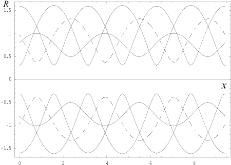
Figure 2: The solutions portrait of system (3.1) with initial value $(R(0),R^{\prime}(0))=\tilde{P}_{i},i=1,2,\cdots,8$. Here, we take $g(x)=\frac{1}{2}-\frac{3}{2}\sin 2x,V(x)=2\sin 2x-1$ and the parameters $\delta=1,c=0.5,\varepsilon=0.01$. These solutions are a good approximation to the periodic orbits for $x$ of order $1/\varepsilon$. The solutions with solid lines are instable.

Using the transformation $\Psi$, these equilibrium points in the $(R,S)$-coordinates with $x=0$ are given by

$$\tilde{P}_{1,2} :(\pm 1.60,0),~{}~{}~{}~{}~{}~{}~{}~{}~{}~{}\tilde{P}_{3,4}:(\pm 0.31,~{}0),~{}~{}$$

$$\tilde{P}_{5,6} :(\pm 0.80,~{}\pm 0.48),~{}~{}\tilde{P}_{7,8}:(\pm 0.98,~{}\mp 0.82).$$

We plot the solutions of system (3.1) starting from $\tilde{P}_{i},i=1,2,\cdots,8$, according to the averaged theorem, which are a good approximation to the periodic orbits, see Figure 2.

6 Conclusion

In conclusion, we have presented first-order averaging theorem in the periodic case for dynamics of MAWs (or QMAWs) in collisionally inhomogeneous BECs. The transformed system is non-Hamiltonian, and we indicate how the averaging theorems can be used to prove the existence and stability of periodic solutions. The questions as mentioned in the introduction have been answered. When the sufficiently small scattering length $a(x)$ varies periodically in spatial variable $x$ and crosses zero, infinitely many (positive measure set) MAWs and QMAWs can be proved to exist by adjusting the integration constant $c$ on some open interval.

A numerical approximation of periodic orbits is given for some prescribed parameters. We remark that, expanding at each equilibrium point and combining with multiple scale perturbed theory, such as work in [24, 6, 25, 26], there may be a better approximation for each continuation periodic orbit. However, we emphasis on the theory frame of averaging to study dynamics of collisionally inhomogeneous BECs.

In the end, it should be remember that the asymptotic approximation are valid for small $\varepsilon$, but how small is usually a difficult problem. However, one advantage of averaging is obvious that it is set up for an easy return to the original variables.

References

• Anderson et al. [1995] M. H. Anderson, J. R. Ensher, M. R. Matthews, C. E. Wieman, E. A. Cornell, Observation of Bose-Einstein condensation in a dilute atomic vapor, science 269 (5221) (1995) 198.
• Davis et al. [1995] K. B. Davis, M. O. Mewes, M. R. Andrews, N. J. Van Druten, D. S. Durfee, D. M. Kurn, W. Ketterle, Bose-Einstein condensation in a gas of sodium atoms, Phys. Rev. Lett. 75 (22) (1995) 3969–3973.
• Strecker et al. [2002] K. E. Strecker, G. B. Partridge, A. G. Truscott, R. G. Hulet, Formation and propagation of matter-wave soliton trains, Nature 417 (6885) (2002) 150–153.
• Strecker et al. [2003] K. E. Strecker, G. B. Partridge, A. G. Truscott, R. G. Hulet, Bright matter wave solitons in Bose–Einstein condensates, New J. Phys. 5 (2003) 73.
• Kevrekidis et al. [2003] P. G. Kevrekidis, G. Theocharis, D. J. Frantzeskakis, B. A. Malomed, Feshbach resonance management for Bose-Einstein condensates, Phys. Rev. Lett. 90 (23) (2003) 230401.
• Porter and Kevrekidis [2005] M. A. Porter, P. G. Kevrekidis, Bose-Einstein Condensates in Superlattices, SIAM J. Appl. Dyn. Syst. 4 (4) (2005) 783–807.
• Kapitula [1998] T. Kapitula, Stability criterion for bright solitary waves of the perturbed cubic-quintic Schrödinger equation, Physica D 116 (1-2) (1998) 95–120.
• Zharnitsky and Pelinovsky [2005] V. Zharnitsky, D. Pelinovsky, Averaging of nonlinearity-managed pulses, Chaos 15 (2005) 037105.
• Cornish et al. [2000] S. L. Cornish, N. R. Claussen, J. L. Roberts, E. A. Cornell, C. E. Wieman, Stable^$\{$85$\}$ Rb Bose-Einstein Condensates with Widely Tunable Interactions, Phys. Rev. Lett. 85 (9) (2000) 1795–1798, ISSN 1079-7114.
• Inouye et al. [1998] S. Inouye, M. R. Andrews, J. Stenger, H. J. Miesner, D. M. Stamper-Kurn, W. Ketterle, Observation of Feshbach resonances in a Bose–Einstein condensate, Nature 392 (6672) (1998) 151–154.
• Porter et al. [2007] M. A. Porter, P. G. Kevrekidis, B. A. Malomed, D. J. Frantzeskakis, Modulated amplitude waves in collisionally inhomogeneous Bose-Einstein condensates, Physica D 229 (2) (2007) 104–115.
• Rapti et al. [2007] Z. Rapti, P. Kevrekidis, V. Konotop, C. Jones, Solitary waves under the competition of linear and nonlinear periodic potentials, Journal of Physics A: Mathematical and Theoretical 40 (2007) 14151.
• Theocharis et al. [2005] G. Theocharis, P. Schmelcher, P. Kevrekidis, D. Frantzeskakis, Matter-wave solitons of collisionally inhomogeneous condensates, Physical Review A 72 (3) (2005) 033614.
• Pelinovsky and Zharnitsky [2003] D. E. Pelinovsky, V. Zharnitsky, Averaging of dispersion-managed solitons: Existence and stability, SIAM J. Appl. Math. 63 (3) (2003) 745–776.
• Pelinovsky et al. [2004] D. Pelinovsky, P. Kevrekidis, D. Frantzeskakis, V. Zharnitsky, Hamiltonian averaging for solitons with nonlinearity management, Phys. Rev. E 70 (4) (2004) 047604.
• Brusch et al. [2000] L. Brusch, M. G. Zimmermann, M. Van Hecke, M. Bär, A. Torcini, Modulated amplitude waves and the transition from phase to defect chaos, Phys. Rev. Lett. 85 (1) (2000) 86–89.
• Brusch et al. [2001] L. Brusch, A. Torcini, M. Van Hecke, M. G. Zimmermann, M. Bär, Modulated amplitude waves and defect formation in the one-dimensional complex Ginzburg-Landau equation, Physica D 160 (3-4) (2001) 127–148.
• Bronski et al. [2001] J. C. Bronski, L. D. Carr, B. Deconinck, J. N. Kutz, Bose-Einstein condensates in standing waves: The cubic nonlinear Schrödinger equation with a periodic potential, Phys. Rev. Lett. 86 (8) (2001) 1402–1405.
• Chong et al. [2004] G. Chong, W. Hai, Q. Xie, Spatial chaos of trapped Bose-Einstein condensate in one-dimensional weak optical lattice potential, Chaos 14 (2004) 217–223.
• Qian and Liu [2011] D. Qian, Q. Liu, Modulated amplitude waves with nonzero phases in Bose-Einstein condensates, arXiv:1103.5277v1 (2011) 1–14.
• Berglund [2001] N. Berglund, Perturbation Theory of Dynamical Systems, Citeseer, 2001.
• Guckenheimer and Holmes [1983] J. Guckenheimer, P. Holmes, Nonlinear Oscillations, Dynamical Dystems and Bifurcations of Vector Fields, Springer-Verlag, 1983.
• Mawhin [1975] J. Mawhin, Topological Degree Method in Nonlinear Boundary Value Problems. CMBS 40,, Amer. Math. Soc., Providence, R.I., 1975.
• Porter and Cvitanovic [2004] M. A. Porter, P. Cvitanovic, A perturbative analysis of modulated amplitude waves in Bose-Einstein condensates, Chaos 14 (2004) 739–755.
• Porter and Cvitanović [2004] M. A. Porter, P. Cvitanović, Modulated amplitude waves in Bose-Einstein condensates, Phys. Rev. E 69 (4) (2004) 047201.
• Porter et al. [2004] M. A. Porter, P. G. Kevrekidis, B. A. Malomed, Resonant and non-resonant modulated amplitude waves for binary Bose-Einstein condensates in optical lattices, Physica D 196 (1-2) (2004) 106–123.