Classes of fast and specific search mechanisms for proteins on DNA

Abstract

Problems of search and recognition appear over different scales in biological systems. In this review we focus on the challenges posed by interactions between proteins, in particular transcription factors, and DNA and possible mechanisms which allow for a fast and selective target location. Initially we argue that DNA-binding proteins can be classified, broadly, into three distinct classes which we illustrate using experimental data. Each class calls for a different search process and we discuss the possible application of different search mechanisms proposed over the years to each class. The main thrust of this review is a new mechanism which is based on barrier discrimination. We introduce the model and analyze in detail its consequences. It is shown that this mechanism applies to all classes of transcription factors and can lead to a fast and specific search. Moreover, it is shown that the mechanism has interesting transient features which allow for stability at the target despite rapid binding and unbinding of the transcription factor from the target.

Contents

1. I Introduction
2. II Protein-DNA energetics
   1. II.1 Target occupation probability in equilibrium
   2. II.2 Experimental data
3. III The search dynamics
   1. III.1 Searching with three-dimensional diffusion
   2. III.2 Searching with one-dimensional diffusion
   3. III.3 Facilitated diffusion
4. IV The speed-stability paradox and possible solutions
   1. IV.1 The speed-stability paradox
   2. IV.2 Possible solutions of the speed-stability paradox for gapped, marginally gapped and non-gapped TFs.
      1. IV.2.1 Gapped TFs
      2. IV.2.2 Two-state models
      3. IV.2.3 Multiple TFs
5. V Search and recognition based on a barrier discrimination – effects of multiple time scales
   1. V.1 Non disordered case
      1. V.1.1 Large barrier regime
   2. V.2 Several searching proteins
   3. V.3 Calculating the average and typical search times
      1. V.3.1 Typical search time
      2. V.3.2 Average search time
   4. V.4 Disordered case
      1. V.4.1 Mean-field analysis
      2. V.4.2 Numerical results and comparison to mean-field analysis
6. VI Effective model and outcomes
   1. VI.1 Transient behavior
   2. VI.2 Steady-state and an existence of an active process
   3. VI.3 The possibility of the genetic temporal ordering
7. VII Summary
8. A An information theoretic approach to the calculation of disorder parameters and binding energies
   1. A.1 The information content and the disorder strength
   2. A.2 The sequence score and the binding energy
9. B A derivation of Eqs. (65) and (66)
10. C Specificity
11. D Details of the simulations
12. E Pole structure analysis and derivation of Eq. (69)
13. F Conditions for a perfect search

I Introduction

Many biochemical processes require both an appropriate speed and a high specificity for proper biological functions to occur – a fast desirable process should not be accompanied by a significant acceleration of undesirable ones. With typical energy scales of a few $k_{B}T$, where $k_{B}$ is the Boltzmann constant and $T$ is the temperature, evolution has devised many efficient mechanisms which overcome the noisy environment and the speed requirements. These range from mechanisms which rely on the consumption of chemical energy, such as kinetic proofreading Hopfield74 , to cooperativity, such as in the specific regulation of the hemoglobin oxygen concentration Hill36 ; Fersht . Unraveling these mechanisms is an important step towards understanding how cells function.

Being based on biopolymers, specificity in biological systems implies that two (or more) well defined subsequences of two given polymers attach to each other, but not to other subsequences of the same polymers or to other polymers. The two polymers can be proteins (for example, in enzymes Fersht ), RNA molecules (for example, in ribosomal action Schimmel98 ; Cech2000 ), a single-stranded and a double stranded DNA (for example, in the homologous recombination Kupiec2008 ) or a transcription factor (TF) and a DNA molecule. The last example highlights the challenges which a biological system faces.

Consider, for example, a prokaryotic cell (throughout the review we focus on these simpler systems). Its typical DNA length is $N\simeq 10^{7}$ basepairs. In a particularly simple case a TF has to bind to a specific subsequence (target) of a length of about $10-20$ basepairs on the DNA. The typical binding energy between a protein and the DNA subsequence is of the order of tens of $k_{B}T$, about one $k_{B}T$ per base-pair. Without using chemical energy (which is true for almost all transcription factors) this gives rise to a classical conflict between entropy and energy which puts a hamper on the stability of the TF at the target. Specifically, the entropy associated with the protein bound to non-target DNA is $k_{B}\ln N\simeq 16k_{B}$ and therefore its contribution to the free energy is of the same order as the binding energy. Unless the TF is designed to have a binding energy at the target that is much lower than to the rest of the sequence the probability of finding it on the target site will be very low. Of course, the copy number of a TF, which in a cell typically ranges from about tens to thousands Guptasarma95 ; RMC98 ; AbundanceDatabase ; AbundanceDatabase2 , can increase the occupation probability of the target site to a desired level (see, for instance, CspA ). This, however, comes at a cost of producing many proteins and possibly activating or repressing unwanted genes and loosing specificity, meaning that the TF is likely to occupy nonspecific sites (below this argument in presented in a quantitative manner).

Following this line of thought early works BWH81 ; HB89 ; HM2004 considered designed targets with a gapped binding energy which is much lower than the rest of the DNA sequence. A sufficiently large energy gap at the target can then yield an arbitrarily large occupation probability of the target site even for one TF. When this is assumed the interesting question becomes that of the speed of the search. To address this question various mechanisms, collectively called facilitated diffusion, were suggested. These combine one dimensional diffusion along the DNA with three-dimensional diffusion or intersegmental transfers. The combination of the various search modes has been observed experimentally BB76 ; winter2 ; WBH81 ; JWSP96 ; JP98 ; BGZY99 ; S99 ; SSMH2000 ; W2005 ; GWH2005 ; WAC2006 ; ELX2007 ; Bonnet2008rp ; Fok2008 ; Loverdo:2009a ; Fok2009 ; hopUL42 and shown theoretically to be capable of decreasing the search time significantly AD68 ; BB76 ; BWH81 ; LKWCJ93 ; GMH2002 ; B2002 ; HM2004 ; SM2004 ; CBVM2004 ; BZ2004 ; K2005 ; Z2005 ; LAM2005 ; HGS2006 ; HS2007 ; Oshanin2007a ; Eliazar2007 ; kolo2008 ; Lomholt2009 ; Florescu2009 ; Florescu2009a ; Givaty2009 ; Vuzman2010a ; Vuzman2010b ; Vuzman2010c ; Rosa2010 ; benichou2011 ; Kolomeisky2011 . More recently the influence of facilitated diffusion on the noise level in gene regulation was analyzed in Bialek2009 ; Tamari2011 .

However, as realized early Hippe86 the assumption of a designed target is far from obvious. In an alphabet of four letters a target sequence of length $12$, quite common in TFs, will occur with essentially probability one in a random sequence of length $\simeq 10^{7}$. Therefore, for target sequences shorter than $12$ bases, identical and almost identical sequences will occur on the DNA. These competing sites can easily ruin the stability of the target site. Furthermore, as discussed in detail below, these almost identical sequences act as traps JAWMP94 that hinder the search process and lead to an antagonism between the stability of the TF at the target site and the speed of the target location. This problem, raised in WBH81 , is commonly referred to as the speed-stability paradox.

Recently, motivated by new experiments there has been renewed interest in this rather old problem. To date there are now several reviews (some very recent) which cover different aspects of the problem HB89 ; HM2004 ; pccp2008 ; Mirny2009 ; kolo2010 ; rmp2011 . We believe that this review complements these and presents the problem using a somewhat new angle. To this end we give an overview of the current status of the speed-stability paradox and its implications on regulation dynamics. We present the problem using both theoretical considerations and experimental data. As we argue it is preposterous to group all TFs in a single class Wunderlich2009 . Different search mechanisms are likely to apply to different proteins grouping them into different classes. We show that three broad classes can be defined, which we term gapped, marginally gapped and non-gapped transcription factors. The applicability of previously suggested search mechanisms to each of the groups is analyzed in some detail. Using this we turn to discuss in detail a recently proposed barrier controlled search mechanism My3 which can in principle resolve the speed-stability paradox for all classes of proteins. The possibility of such a mechanism suggests that experiments should also probe activation barriers and not, as commonly done, binding energies (see discussion below). Moreover, this mechanism allows for a rich transient behavior and for transcription factors which are efficient despite binding and unbinding rapidly from the target.

The structure of the review is as follows: In Section II we discuss in detail the energetics associated with protein-DNA interaction. We argue for the classification of transcription factors into the three classes defined above. The classification is illustrated using experimental data. In Section III we review the kinetics of simple search mechanisms which have been discussed in the literature. In Section IV we introduce the speed-stability paradox and its possible resolution for each class of TFs. In Section V we introduce and analyze in detail the barrier controlled search mechanism. In Section VI an effective model for the barrier controlled search mechanism is introduced and used to study transient behaviors. We summarize the results in Sec. VII.

II Protein-DNA energetics

Due to the sequences heterogeneity of the non-target DNA the binding energy of a protein to a DNA is location dependent. The structure of this disordered, non-specific, energy landscape is crucial for understanding the stability of a TF at its target site and which search strategies can or cannot be efficient. To this end, in this Section we consider the energy landscape both from a theoretical point of view and by looking at experimental data. Throughout what follows we use units where $k_{B}T=1$.

Equilibrium measurements SF98 reveal that to a good approximation the binding energy, $U\left({\bf s}\right)$, of a transcription factor which binds to a sequence of $l_{p}$ bases ${\bf s}=\left(s_{1},s_{2},...,s_{l_{p}}\right)$ on the DNA is given by GMH2002

$$U\left({\bf s}\right)=\underset{i=1}{\overset{l_{p}}{\sum}}\mathcal{E}\left(s_{i},i\right)\;.$$ (1)

Here $s_{i}=A,T,C,G$ is the nucleotide type on the $i$th binding location of the protein and $l_{p}$ is the number of binding sites on the protein (see Fig. 1). The binding energies $\mathcal{E}\left(s,i\right)$ are usually estimated experimentally by measuring the probability, $\Pr\left(s,i\right)$, that a nucleotide $s$ is bound to a location $i$ on the protein in equilibrium in vitro experiments. Namely, one uses

$$\Pr\left(s,i\right)=\frac{e^{-\mathcal{E}\left(s,i\right)}}{Z_{i}}\;\;\;\;{\rm where}\;\;\;\;\;Z_{i}=\underset{s^{\prime}=\left\{A,T,C,G\right\}}{\sum}e^{-\mathcal{E}\left(s^{\prime},i\right)}.$$ (2)

The matrix $\Pr\left(s,i\right)$ has $4\times l_{p}$ elements and is called the weight matrix (also known as Position-Specific Scoring Matrix (PSSM) or "profile"). It is important to note that these probabilities are measured only for sequences which are close in structure to the target site. The reason for this lies in the existence of other conformations of the protein-DNA complex which we will allude to later Quake2007 . In Fig. 2 we illustrate a sample binding energy probability distribution for several E. coli proteins.

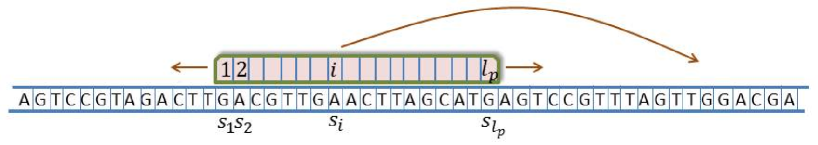
Figure 1: In this cartoon the interaction between the transcription factor of length $l_{p}$ and the DNA sequence s is illustrated.

The structure of the binding energy implies that it can be described by three parameters instead of the $4^{l_{p}}$ entries. Specifically, the energy is a sum of contributions (see Eq. (1)) which can be assumed independent, if the DNA sequence is uncorrelated, and can therefore be modeled to a good approximation by a Gaussian random variable. (The assumption that the DNA sequence is uncorrelated is believed to be true for coding DNA and in particular for prokaryotic DNA.) The validity of this approximation is illustrated for several proteins in Fig. 3. As can be seen it holds for energies above the target energy, $U_{\mathcal{T}}$, which is defined as the lowest possible binding energy of the TF to any sequence. Explicitly, the probability density of finding a given binding energy $U$ for non-target sequences is well approximated by

$$P(U)\simeq\left\{\begin{array}[]{cc}{\cal N}^{-1}e^{-\frac{U^{2}}{2\sigma_{U}^{2}}}&U>U_{\mathcal{T}}\\ 0&U<U_{\mathcal{T}}\end{array}\right.,$$ (3)

where ${\cal N}$ is a normalization factor and the variance

$$\sigma_{U}^{2}=\underset{i=1}{\overset{l_{p}}{\sum}}\left\{\underset{s_{i}=\left\{A,T,G,C\right\}}{\frac{1}{4}\sum}\mathcal{E}^{2}\left(s_{i},i\right)-\left[\underset{s_{i}=\left\{A,T,G,C\right\}}{\frac{1}{4}\sum}\mathcal{E}\left(s_{i},i\right)\right]^{2}\right\}\;.$$ (4)

The target energy is given by:

$$U_{\mathcal{T}}=\underset{i=1}{\overset{l_{p}}{\sum}}\min\left[\mathcal{E}\left(A,i\right),\mathcal{E}\left(T,i\right),\mathcal{E}\left(C,i\right),\mathcal{E}\left(G,i\right)\right].$$ (5)

The statistical properties of the binding energy are now encoded by $\sigma_{U}$ and $U_{\mathcal{T}}$ and the mean binding energy which we set to be zero. Note, that the Gaussian form is unchanged even if one allows for corrections to the weight matrix which depend, say, on near-neighbor configurations, as suggested in Stormo86 ; Zhang93 ; Ponomarenko99 ; Bulyk2002 . The assumption that the DNA sequence is uncorrelated also implies that the binding energies $U_{i}$ and $U_{j}$ at different sites $i$ and $j$ are independent. Strictly speaking this holds only for $|i-j|>l_{p}$. In what follows we neglect these, unimportant, short range correlations.

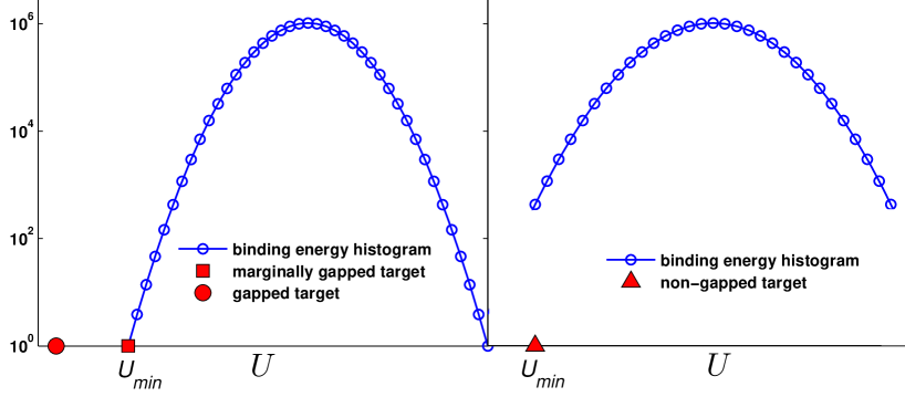
Figure 2: In this schematic plot three different types of a target are shown for a given binding energy histogram (blue curve).

Another quantity which is important for understanding the binding is the minimal energy, $U_{min}\geq U_{\cal T}$, which occurs randomly on a typical DNA sequence among the non-target sites. This site competes most strongly with the target site. In a sequence of $N\gg 1$ uncorrelated base pairs, it is narrowly distributed (with a variance scaling as $1/\ln N$) and well approximated by HF2006

$$\int_{-\infty}^{U_{min}}P(U)\simeq\frac{1}{N}$$ (6)

or

$$U_{min}\simeq\max\left(-\sigma_{U}\sqrt{2}\operatorname{erfc}^{-1}\left(\frac{2}{N}\right),U_{\mathcal{T}}\right)\simeq\max\left(-\sigma_{U}\sqrt{2\ln N},U_{\mathcal{T}}\right).$$ (7)

For a given DNA length, $N$, $U_{min}$, $U_{\cal T}$ and $\sigma_{U}$ characterize the binding properties of a TF. This naturally leads to three classes of transcription factors (see Fig. 2 for a schematic illustration).

Gapped transcription factors.

In this case there is a significant gap between the lowest non-target energy, $U_{min}$, and the target energy, $U_{{\cal T}}$. Namely,

$$U_{min}\simeq-\sigma_{U}\sqrt{2\ln N}$$ (8)

and

$$U_{\mathcal{T}}<-\sigma_{U}\sqrt{2\ln N}.$$ (9)

Marginally gapped transcription factors.

Here there is no energetic gap between the target and the rest of the DNA but the number of sites with an energy close to $U_{{\cal T}}$ is small (of the order of one). This happens when

$$U_{min}\simeq U_{\mathcal{T}}\simeq-\sigma_{U}\sqrt{2\ln N}.$$ (10)

Non-gapped transcription factors.

In this case there is no energetic gap between the target and the rest of the DNA and the number of sites with an energy close to the target one is large. This happens when

$$U_{min}\simeq U_{\mathcal{T}}>-\sigma_{U}\sqrt{2\ln N}.$$ (11)

Note that within the additive binding energy model, Eq. (1), the possible existence of a gapped TF is directly related to its length. In that case

$$U_{{\cal\mathcal{T}}}=l_{p}E_{c}$$ (12)

where $E_{c}<0$ is the average lowest binding energy per base and

$$\sigma_{U}^{2}=\frac{l_{p}E_{c}^{2}}{3}.$$ (13)

Here we assumed that each base appears with equal probability along the DNA. Then Eq. (9) implies that to produce an energetic gap between $U_{\mathcal{T}}$ and $U_{min}$ a TF has to be long enough. Namely, one finds

$$l_{p}>\frac{2}{3}\ln N\;.$$ (14)

This has a particularly simple interpretation. It is equivalent to demanding that on a DNA sequence, of length $N$, sites which are identical to the target site do not appear randomly so that $1/4^{l_{p}}<1/N$. For a typical bacterial DNA length, $N=10^{7}$, this gives $l_{p}>11$. The argument can be refined using information theoretic arguments (see Appendix A and for a similar line of reasoning Wunderlich2009 ) to give a stronger bound of $l_{p}>22$.

As we discuss below, the structure of the energy landscape, gap existence and the properties of the target have important consequences on the equilibrium probability of finding the protein on the target and the search time. Interestingly, as we show below, experimental data suggests that there are transcription factors which belong to each of the above categories.

II.1 Target occupation probability in equilibrium

Next, we turn to consider the probability of a TF to be at the target, $P^{\mathcal{T}}$, in equilibrium. For TFs which appear in small numbers (as believed to be the case in many examples Guptasarma95 ) this quantity has to be of the order of one for proper control over gene expression. Otherwise, assuming equilibration (we discuss other scenarios later), the TF has to be present in a large copy number. Naively $P^{\mathcal{T}}$ will be of the order of one as long as the TF is gapped. As we now show this is not guaranteed and we outline the conditions for this to occur. We ignore the free-energy contribution from configurations where the protein is off the DNA. These can only hamper the stability at the target.

In equilibrium to ensure $P^{\mathcal{T}}$ close to one the partition function has to be dominated by the target energy. Namely, for stability we require

$$Z=\sum_{i=1}^{N}e^{-U_{i}}\simeq e^{-U_{\mathcal{T}}}.$$ (15)

The typical partition function can be approximated, using Eq. (3), by

$$Z\simeq e^{-U_{{\cal\mathcal{T}}}}+N\frac{\underset{U_{min}}{\overset{\infty}{\int}}e^{-\frac{U^{2}}{2\sigma_{U}^{2}}}e^{-U}dU}{\underset{U_{min}}{\overset{\infty}{\int}}e^{-\frac{U^{2}}{2\sigma_{U}^{2}}}dU}.$$ (16)

Note, that as standard in disordered systems, this can be different from the average partition function which is obtained by setting the lower bound of the integrations on the right hand side to $-\infty$. This gives in the large $N$ limit

$$Z \simeq\left\{\begin{array}[]{cc}e^{-U_{{\cal\mathcal{T}}}}+e^{\sigma_{U}\sqrt{2\ln N}}&\ {\rm for}\ \sigma_{U}\gg\sqrt{2\ln N}\\ e^{-U_{{\cal\mathcal{T}}}}+Ne^{\frac{\sigma_{U}^{2}}{2}}&\ {\rm for}\ \sigma_{U}\ll\sqrt{2\ln N}\end{array}\right..$$ (19)

We therefore identify two regimes: large disorder strength $\sigma_{U}\gg\sqrt{2\ln N}$ and small disorder strength $\sigma_{U}\ll\sqrt{2\ln N}$. Note, that the physics is very close to that of the Random Energy Model (REM) Derrida1980 .

For large disorder strength $\sigma_{U}\gg\sqrt{2\ln N}$, which corresponds to the frozen phase of the REM, gapped TFs or marginally gapped TFs are stable on the target. Together with the definitions (9)-(10), this condition reads

$$U_{{\cal\mathcal{T}}}\leq-\sigma_{U}\sqrt{2\ln N}\;.$$ (20)

To satisfy the stability requirement in the small disorder case, which corresponds to a system above the freezing point of the REM, it is required that

$$U_{{\cal\mathcal{T}}}\leq-\ln N-\sigma_{U}^{2}/2\;,$$ (21)

so that only gapped TFs can be stable on the target. Using the additive binding model, so that $U_{{\cal\mathcal{T}}}=l_{p}E_{c}$ and $\sigma_{U}^{2}=\frac{l_{p}E_{c}^{2}}{3}$ implies that the small disorder regime corresponds to $l_{p}\ll\frac{6\ln N}{E_{c}^{2}}$ and the stability condition translates in this case to the constraint

$$l_{p}\geq\frac{\ln N}{-E_{c}(1+E_{c}/6)}.$$ (22)

This is possible only for $-E_{c}<6$. As expected the bound on $l_{p}$ grows when $E_{c}$ approaches zero.

Note that for both large and small disorder strengths, the larger $N$, the more stringent the condition on $U_{{\cal\mathcal{T}}}$. With $E_{c}$ of the order of $-1$ the above conditions give $l_{p}\geq 16$ for small disorder and $l_{p}\geq 32$ for large disorder. We comment, that in principle a simple way to satisfy the conditions (20) or (21), is for example to introduce large enough cooperative interactions between different TF’s binding domains. In this case the binding energy is not additive so that Eq. (1) is not valid. These can single out the target and generate an arbitrarily large gap between the target and the rest of DNA sites.

In summary, TFs with non-gapped targets cannot be stabilized on their targets. Marginally gapped TFs can be stabilized on their targets if the disorder strength is large enough. Below, we show that this requirement gives rise to a conflict with the speed of the target location. A gapped TF is stable on its target when the disorder strength is large, or in the small disorder regime if it is large enough (or if cooperative effects are present). Without any cooperative interaction between different TF’s parts, such a gap may be achieved in both small and large disorder regimes for reasonable TF’s length (for a biochemically reasonable energy scale of about $1$). Below we show that combining these requirements with another set of constraints related to the speed of the search gives much more stringent conditions on the length of the protein.

II.2 Experimental data

In recent years much experimental data has been accumulated. Specifically the weight matrix has been measured for many TFs. We now use data from RegulonDB regulonDB which contains 89 weight matrices to try and single out the different classes of proteins discussed theoretically above. As we proceed to show, the three classes can be identified in the data. Three examples are shown in Fig. 3. These correspond to a gapped (Fig. 3(a)), marginally gapped (Fig. 3(b)) and non-gapped (Fig. 3(c)) proteins.

To analyze the stability of all the proteins in the database we look at several quantities. (i) Their minimal possible binding energy $U_{{\cal\mathcal{T}}}=U({\bf s}^{*})$, where ${\bf s}^{*}$ is defined to be the target of the protein. (ii) The minimal binding energy on a typical disordered sequence of length $N$, $U_{min}=U({\bf s}^{\dagger})$, where ${\bf s}^{\dagger}$ is the strongest binder on the sequence. (iii) The standard deviation $\sigma_{U}$ for the different proteins and finally (iv) the occupation probability at the target, $P^{\mathcal{T}}$. Some of the results presented below are demonstrated in Appendix A using the language of information theory (for a related discussion see Wunderlich2009 ).

It is useful to present that data by plotting $U_{min}$ and $U_{{\cal\mathcal{T}}}$ as a function of $\sigma_{U}$ (see Fig. 4). Each protein on the graph is represented by two points with the same abscissa. The graph shows several interesting features.

(i) First, as expected, a significant part (about three fourth) of the TFs are gapped with a gap size ranging from a few $k_{B}T$ to about $20k_{B}T$. A histogram of the gap size is shown in Fig. 3(d). As stated above such gapped proteins are stable only when the gap is large enough, see Eqs. (21) and (20). For an E. coli DNA length this requires $U_{\cal T}<-15$ in the small disorder regime ($\sigma_{U}\ll\sqrt{2\ln N}\simeq 5.5$) and $U_{\cal T}<-30$ in the large disorder regime ($\sigma_{U}\gg 5.5$). Note that indeed for $\sigma\geq 5.5$ a large fraction of the values of $U_{\cal T}$ are below $-30$ and therefore correspond to stable TFs. The stability criterions for both small (Eq. (21)) and large (Eq. (20)) disorder strengths are shown in Fig. 5 and indicate that most proteins with a large gap are stable. Note also that the theoretical prediction for $U_{min}$ (shown in Fig. 4) fits reasonably well with the experimental results.

(ii) Second, for about one fourth of the TFs $U_{\cal T}\simeq U_{min}$. This indicates that they are either non-gapped or marginally gapped. Recall that for such proteins a minimal criterion for being stable at the target is that the disorder is large ($\sigma_{U}\geq\sqrt{2\ln N}\simeq 5.5$). This does not seem to be satisfied for most of the marginally gapped proteins. Therefore, Fig. 4 hints that most of the non gapped and marginally gapped TFs are actually unstable on the target. This is more clearly illustrated in Fig. 6 which shows that indeed about one quarter of the proteins have a very small probability (less than $10^{-1}$ with about half of them with a probability less than $10^{-2}$) for being on the target. This indicates that non gapped and marginally gapped TFs seem to break the stability requirement. We return to these proteins later and suggest that either non-equilibrium effects or large copy numbers could stabilize them on the target.

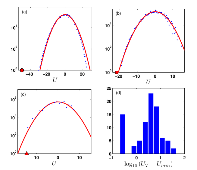
Figure 3: Here a histogram of the binding energy is presented for three different TFs. (a) BaeR, $l_{p}=29$, $\sigma=6.86$, $U_{{\cal\mathcal{T}}}=-50.16$, $E_{min}=-33.5$, $P^{\mathcal{T}}=1$. (b) DcuR, $l_{p}=15$, $\sigma=4.93$, $U_{{\cal\mathcal{T}}}=-21.76$, $E_{min}=-21.75$, $P^{\mathcal{T}}=0.074$. (c) AscG, $l_{p}=7$, $\sigma=4.2$, $U_{{\cal\mathcal{T}}}=-14.55$, $E_{min}=-14.55$, $P^{\mathcal{T}}=0.0006$. The red lines are Gaussian approximations to the distributions using the measured variance calculated from Eq. (4). (d) A histogram of the estimated gap values. The data is based on 89 weight matrices of E. coli DNA-binding proteins and was taken from the RegulonDB database regulonDB .

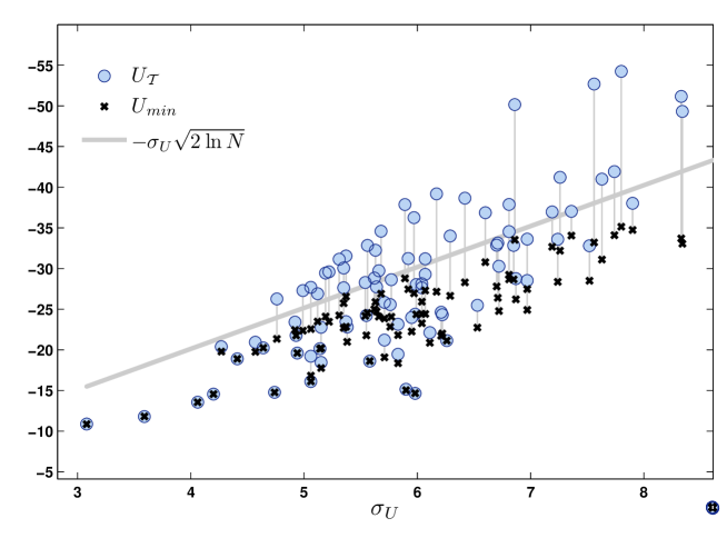
Figure 4: On this figure a comparison between (gray, thick, solid line) the analytic upper limit for a minimal non-designed binding energy Eq. (7), (black crosses) the estimated minimal non-designed binding energy, $U_{min}$ and (blue circles) the estimated binding energy of a perfectly designed full consensus sequence, $U_{{\cal\mathcal{T}}}$. Each $\sigma_{U}$ corresponds to a different protein. The data is based on $89$ weight matrices of E. coli DNA-binding proteins and was taken from the RegulonDB database regulonDB .

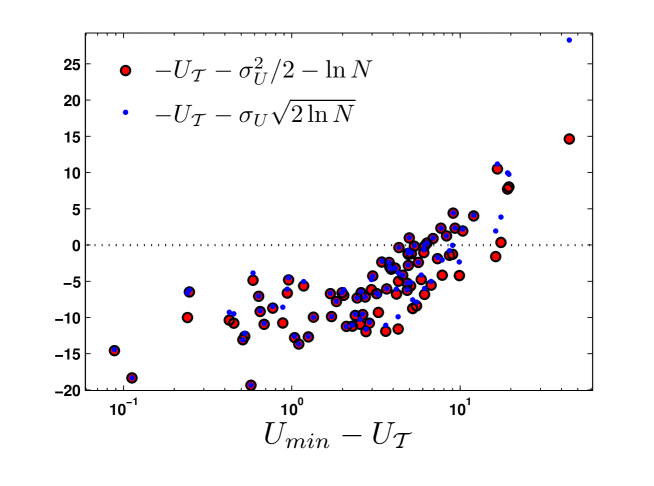
Figure 5: The stability criterions in the small (Eq. (21), large red dots) and large (Eq. (20), small blue dots) disorder regimes. The data is based on $89$ weight matrices of E. coli DNA-binding proteins and was taken from the RegulonDB database regulonDB .

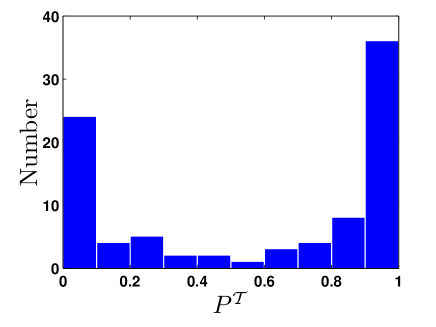
Figure 6: Here a histogram of the occupation probability of a target, $P^{\mathcal{T}}$, is presented. The bulk term was not taken into account such that the presented data slightly overestimate $P^{\mathcal{T}}$. The data is based on $89$ weight matrices of E. coli DNA-binding proteins and was taken from the RegulonDB database regulonDB .

It is interesting to present the same data, but instead of as a function of $\sigma_{U}$, as a function of $l_{p}$. This is shown in Figs. 7 and 8. As is clearly seen there is a close relation between the existence of a gap and $l_{p}$ being large enough. In fact, in agreement with our simple arguments, a gap begins to form at $l_{p}\simeq 13$. The data for $P^{\cal T}$ as a function of $l_{p}$ is even more striking. Essentially all proteins with a binding site of size $l_{p}\simeq 13$ or smaller are unstable on the target while those with $l_{p}\simeq 16$ or larger are mostly stable at the target. The close correspondence between $l_{p}$ and the gap is a direct result of a similar binding energy per base for all TFs.

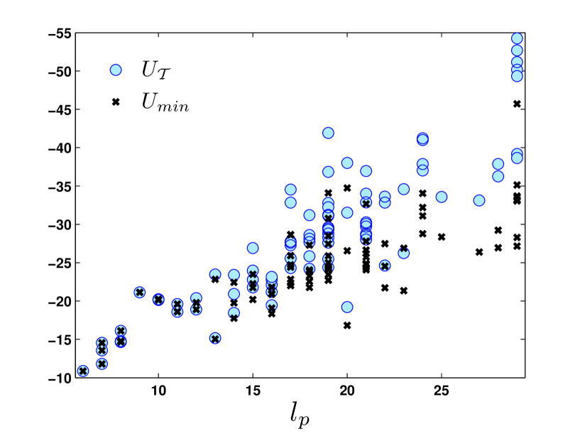
Figure 7: A comparison between (black crosses) the estimated minimal non-designed binding energy, $U_{min}$ and (blue circles) the estimated binding energy of a perfectly designed full consensus sequence, $U_{{\cal\mathcal{T}}}$ as a function of the protein’s length. The data is based on $89$ weight matrices of E. coli DNA-binding proteins and was taken from the RegulonDB database regulonDB .

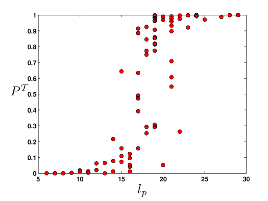
Figure 8: The occupation probability of a target, $P^{\mathcal{T}}$, is presented as a function of a protein’s length, $l_{p}$. The bulk term was not taken into account such that the presented data slightly overestimate $P^{\mathcal{T}}$. The data is based on $89$ weight matrices of E. coli DNA-binding proteins and was taken from the RegulonDB database regulonDB .

The above discussion focused on the stability characteristics. We identified several distinct classes of TFs based on their stability properties. An important question for transcription factors is their speed of operation. The discussion above suggests that different TFs could have different search strategies. Before attempting to map these out in what follows we first review the different possible reactive pathways which have been suggested in the literature.

III The search dynamics

Before discussing the reactive pathways it is useful to have a simple picture of DNA packing in prokaryotic cells. In typical systems the DNA has a total length of $L\sim 10^{6}nm$, a persistence length $L_{0}\sim 50nm$, a cross section radius $\rho\sim 1nm$, and is contained in a volume of $\Lambda^{3}\sim 10^{9}nm^{3}$. The typical distance between segments of DNA of length $L_{0}$ is therefore much smaller than $L_{0}$: $\frac{\Lambda^{3}}{L/L_{0}}\ll L_{0}^{3}$. Under these conditions, using $\Lambda\gg L_{0}$, it is easy to check that the radius of gyration of free DNA, which is of the order of $L_{0}\sqrt{\frac{L}{L_{0}}}$ is much larger than the cell size $\Lambda$ - the DNA is densely packed even though its fractional volume in the container $L\rho^{2}/\Lambda^{3}$, is small (about one percent). By way of comparison, typical protein sizes are in the range $R\mathbf{\sim}1-10nm$, much smaller than the DNA’s persistence length.

To quantify the search process one needs to estimate the time it takes the protein, from its initial production, to activate (or repress) its target site. Early works considered a perfectly reactive target. In this case the search efficiency can be quantified by studying the statistical properties of the first-passage time to the target R2001 ; nature2007 ; natchem2010 . In this section we focus on the mean first-passage time. Later, we will discuss the potential importance of other time scales in the problem.

For a cell to properly function the search process has to, typically, be of the order of seconds. In principle, when the target is perfectly reactive this can be achieved by a search which is driven by pure three dimensional diffusion. However, driven by experimental results, mostly on the Lac repressor RSB70 ; RBC70 , which seem to give search times that are faster than three-dimensional diffusion, various search strategies were suggested. We now give simple arguments that quantify these different search strategies. For a similar discussion see SM2004 ; HGS2006 .

III.1 Searching with three-dimensional diffusion

Naively, one might expect the protein to search for its target (or, equivalently, its specific binding site on the DNA) using only three-dimensional diffusion. Neglecting interactions of the protein with the environment and the DNA (apart from the target site), one then finds, using results first obtained by Smoluchowski S17 or by dimensional analysis, that the search time, $t^{search}$, defined as the mean first-passage time at the target, is given by:

$$t^{search}\sim\frac{\Lambda^{3}}{D_{3}r}.$$ (23)

Here $D_{3}$ is the three-dimensional diffusion constant of the protein, $r$ is the target size, and $\Lambda^{3}$ is the volume that needs to be searched. Assuming a target size of the order of a base-pair $r\approx 0.34nm$, a typical nucleus (or bacterium) size as above and using the measured three-dimensional diffusion coefficient for a GFP protein in vivo, $D_{3}\sim 10^{7}{nm}^{2}/s$ ESWSL99 , one finds $t^{search}$ of the order of hundreds of seconds. We comment that $r$ can be increased significantly by changing the electrostatic interactions between the protein and its target, for example, by changing the salt concentration.

These long time scales can be easily reduced if several proteins are searching for the target. Namely, if $n_{p}$ proteins are searching for the same target the average search time is given by $t_{n_{p}}^{search}\simeq t^{search}/n_{p}$. This suggests that about $10$ proteins could find a target in reasonable time for cells to function properly. As we discuss below this simple relation between the search time of one protein and $n_{p}$ proteins can fail in some cases.

III.2 Searching with one-dimensional diffusion

In real systems, due to the interactions of proteins with non-specific DNA sequences and the environment LR72 , the picture is more complex. Indeed, in vitro experiments have suggested that mechanisms other than three-dimensional diffusion are used by many proteins to locate their targets. The simplest extension of the pure three-dimensional diffusive search is using three dimensional diffusion to reach the DNA and then scan it using one-dimensional diffusion along its contour. This follows closely ideas of Delbruck and Adam AD68 , introduced in a different context. If the DNA is very long the search time is clearly controlled by the one-dimensional diffusion along the DNA which is given by

$$t^{search}\sim\frac{L^{2}}{D_{1}}\sim O\left(hours\right)\;.$$ (24)

Here $L\sim 10^{6}nm$ is the genome length and $D_{1}$ is the one-dimensional diffusion coefficient that was measured indirectly BB76 and directly WAC2006 ; ELX2007 to be much smaller than the three-dimensional diffusion coefficient $D_{3}\sim 10^{7}nm^{2}/s$ ESWSL99 . Effects of disorder can be incorporated into an effective value of $D_{1}$ SM2004 (see discussion below). The above result renders this search strategy useless for long DNA. However, if the sequence scanned is short then it is easy to see that the search time is given by

$$t^{search}\sim\frac{L^{2}}{D_{1}}+\frac{\Lambda^{3}}{D_{3}L}\;.$$ (25)

Using the numbers cited above it is easy to check that search times of the order of a $100$ sec (so that about 10 proteins can find the target within seconds) can be obtain as long as $L$, the length of the sequence scanned is smaller than $10^{4}$ nm, about $30$ kilobases long. The results are mildly modified if the sequence has a globular shape.

III.3 Facilitated diffusion

Motivated by experiments RSB70 ; RBC70 an extension of the Delbruck and Adam model was suggested in BWH81 . The model combines one-dimensional diffusion (sliding) along the DNA which is interrupted by periods of three dimensional diffusion (typically called jumping or hopping in this context). This combined strategy, called facilitated diffusion, has been studied and debated extensively both in the context of in vivo BWH81 ; SM2004 ; HGS2006 ; HS2007 ; ELX2007 and in vitro systems BB76 ; BWH81 ; Terry85 ; HM2004 ; BZ2004 ; Z2005 ; LAM2005 ; HGS2006 ; Blainey2006 . There is now a large body of evidence that such a mechanism plays an important role for several TFs. It is illustrated in Fig. 9 and is believed to speed the search process.

Each of the individual search mechanisms described above, when applied alone, has shortcomings and advantages over the other. When using only three-dimensional diffusion, the number of distinct three dimensional positions probed grows linearly in time but the protein spends much time probing sites where there is no DNA present. In contrast, during a one-dimensional diffusion the protein is constantly bound to the DNA but suffers from a slow increase in the number of distinct positions probed as a function of time ($\sim t^{1/2}$, where $t$ denotes time) H95Volume1 . It is known that by intertwining one and three dimensional search strategies and tuning the properties of both one can in fact decrease the search time significantly BWH81 .

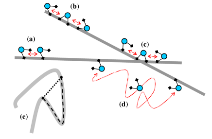
Figure 9: Schematic plots illustrating the different mechanisms that can participate in the facilitated diffusion process. Here dashed arrows represent different protein moves, the solid curve represents the DNA and a small circle with two legs indicates a protein with two binding domains. The figure shows (a) sliding, (b) a correlated intersegmental transfer, (c) an uncorrelated intersegmental transfer, (d) jumping. (e) The dashed (dotted) line represents a one-dimensional (three-dimensional) distance.

The discussion below follows Refs. HM2004 and SM2004 closely. We imagine a single protein searching for a single target located on the DNA. The search is composed of a series of intervals of one-dimensional diffusion along the DNA (sliding) and three-dimensional diffusion in the solution (jumping). The mean time of each is denoted by $\tau_{1}$ and $\tau_{3}$ respectively. Following a jump, the protein is assumed to associate on a new randomly chosen location along the DNA. Note that one might be worried if the structure of the packed DNA molecule invalidates this approach. Numerics on typical frozen DNA conformations indicate that as long as average search times are considered the structure can be ignored SK2009 . Nonetheless much more complicated structures may arise in nature (for example, in eukaryotic cells crumpleddna ; HGS2006 ; Bancaud2009 ; Lieberman-Aiden:2009fk ) and these are ignored in the discussion below.

Under the above assumptions, during each sliding event the protein covers a typical length $l$, where $l\sim\sqrt{D_{1}\tau_{1}}$ (often called the antenna size) H95Volume1 . To complete the search process

$$N_{r}\sim\frac{L}{l}$$ (26)

rounds of sliding and jumping are needed on average. While this can be intuitively understood since the correlations between the locations of the protein before and after the jump are neglected the exact nature of the relation is in fact somewhat more subtle. As shown in CBVM2004 the average length scanned before the target is reached is half the total length. Nonetheless for the average search time the expression is exact in the large $L$ limit. The total time needed to find a specific site is then:

$$t^{search}=N_{r}\tau_{r},$$ (27)

where $\tau_{r}=\tau_{1}+\tau_{3}$ is the typical time of a round. Using Eqs. (26) and (27) one obtains

$$t^{search}\sim\frac{L}{l}(\tau_{1}+\tau_{3})\sim\frac{L}{\sqrt{2D_{1}}}\left(\sqrt{\tau_{1}}+\frac{\tau_{3}}{\sqrt{\tau_{1}}}\right).$$ (28)

Furthermore, from dimensional analysis it is easy to argue that

$$\tau_{3}\sim\frac{\Lambda^{3}}{D_{3}L}.$$ (29)

As shown in nature2007 this result holds up to a logarithmic correction which diverges as the DNAs cross section, $\rho$, vanishes. The analysis leads to three distinct regimes (i) For $\tau_{1}\ll\tau_{3}$ there is no dependence on $L$ and the search time is given to a good approximation by Eq. (23). (ii) For $\frac{L^{2}}{D_{1}}\gg\tau_{1}\gg\tau_{3}$ the dependence on the DNA length is linear. This is the regime typically considered relevant for experiments. (iii) For $\frac{L^{2}}{D_{1}}\ll\tau_{1}$ one finds $t^{search}\propto L^{2}$.

It is natural to ask which $\tau_{1}$ optimizes $t^{search}$ when $\tau_{3}$ is held fixed. Using Eq. (28) it is easy to verify that

$$\tau_{1}^{opt}=\tau_{3}\;.$$ (30)

It can be shown that this result is exact in the large $L$ limit CBVM2004 . Alternatively, one can consider an optimal antenna size $l_{opt}=\sqrt{2D_{1}\tau_{3}}$. When this condition is met, the total search time scales as

$$t_{opt}^{search}=\sqrt{\frac{\tau_{3}}{D_{1}}}L\sim\sqrt{\frac{\Lambda^{3}L}{D_{1}D_{3}}}.$$ (31)

Note that the $\sqrt{L}$ dependence is obtained by optimizing, say $\tau_{1}$, as $L$ is varied. This model, at the optimal $\tau_{1}$ and assuming known values for $D_{1}$, $L$ and $\tau_{3}$, predicts reasonable search times in vivo and is commonly believed to give a possible explanation for the efficiency of the target location process in experiments.

The combined strategy, while better than the pure three-dimensional or one-dimensional search strategies, comes at a cost of being sensitive to changes in the properties of either the three-dimensional or the one-dimensional diffusive processes. Given the many constraints on the protein to function, it is restrictive to demand an optimization of the search process. Specifically, within the model an optimal search process requires fine tuning of the antenna size, $l$, as a function of the parameters $D_{1}$ and $\tau_{3}$. These parameters depend on various cell and environmental conditions such as the size of the cell, the DNA length, the ionic strength etc. The dependence can be quite significant: for example, the parameter $\tau_{3}/\tau_{1}$ has been argued to have an exponential dependence on the square root of the ionic strength LR75 . Deviations of this parameter from the optimum value might be crucial to the search time since $\frac{t^{search}}{t_{opt}^{search}}=\frac{1}{2}\left(\sqrt{\frac{\tau_{3}}{\tau_{1}}}+\sqrt{\frac{\tau_{1}}{\tau_{3}}}\right)$. Indeed, a strong dependence of the search time on the ionic strength was found in in vitro experiments RBC70 .

Interestingly, in vivo, when the DNA is densely packed, no effect of the ionic strength on the efficiency of the Lac repressor was revealed RCMKAFR87 . Other experiments also suggest that $\tau_{1}$ is not optimized. In particular, equilibrium measurements K-HRBOCNVH77 , as well as recent single molecule experiments WAC2006 ; ELX2007 , find a value of $\tau_{1}$ for the Lac repressor that is much larger than the predicted optimum $\tau_{3}$ in vivo. The lack of sensitivity to the ionic strength in vivo and the rapid search times found for the Lac repressor, even with very large values of $\tau_{1}$, suggest that other processes, apart from jumping and sliding, are involved in the search process. These seem to be more important in vivo than in vitro. One such mechanism which was suggested to speed the search time is intersegmental transfers (IT) HRGW75 ; BC75 . During an IT the protein moves from one site to another by transiently binding both at the same time. This mechanism is expected to be important for systems with a high DNA density Broek2008kl . In principle the new site can be either close along the one-dimensional DNA sequence (or chemical distance) or distant (see Fig. 9). An analysis shows that the average search time remains similar to the combined one-dimensional and three-dimensional diffusion described above but with $\tau_{3}$ which obtains a different dependence on the DNA length. This has been discussed in detail in SK2009 .

Finally, we comment that in principle all search strategies can be made arbitrarily fast by increasing the number of searchers. This allows, in principle, any of the above discussed mechanisms, one-dimensional diffusion, three-dimensional diffusion, facilitated diffusion with or without intersegmental transfers, to be at work for different proteins Halford2009 . This statement, however, becomes more problematic when the stability requirements discussed above are included. As stated above, it is clear that the TFs also interact with non-target sites so that pure three dimensional searches are unlikely. This implies that facilitated diffusion is hard to avoid. To this end, in what follows we analyze in detail the problems which arise when facilitated diffusion is combined with the stability requirements.

IV The speed-stability paradox and possible solutions

It has been recognized early that there is a tight connection and antagonism between the stability of the TF at the target and the search speed. The conflict is commonly termed the speed-stability paradox WBH81 ; SM2004 . As we have seen, the experimental data shows that the proteins can be classified into several classes. These classes call for different mechanisms. We begin by introducing the speed-stability paradox and then discuss possible solutions for each class of proteins.

IV.1 The speed-stability paradox

Recall that a fast search of one protein (we later return to the case of $n_{p}$ proteins and discuss it in detail) requires a fast one-dimensional diffusion on the DNA. Then note that the binding energies between the transcription factor and the DNA on each site $i$, $U_{i}$, is an independent random variable with a Gaussian distribution with a variance $\sigma_{U}^{2}$. This disorder in the binding energies of the protein to different sites implies that this diffusion takes place on a disordered potential. On long times this leads to an effective diffusion constant whose value is given by SM2004

$$D_{1}=D_{1}\left(\sigma_{U}=0\right)\sqrt{1+\frac{\sigma_{U}^{2}}{2}}e^{-\frac{7}{4}\sigma_{U}^{2}}.$$ (32)

The important thing to note is the exponential dependence of the diffusion coefficient on $\sigma_{U}^{2}$. It can be understood up to prefactors by recalling that the diffusion is an activated process so that $D_{1}\propto\int dUe^{-U}Pr(U)$ . This implies that even for $\sigma_{U}=5.5$ (the boarder line between the small and the large disorder regimes for an E. coli genome) the one-dimensional diffusion constant becomes $19$ orders of magnitude smaller than the diffusion constant on a flat energy landscape. This in turn leads to a very slow search process. Essentially, speed requirements prohibit the large disorder regime discussed above. For the search to be fast $\sigma_{U}$ has to be kept small, of the order of $0.5$, to ensure a diffusion coefficient of the same order as that on a flat energy landscape.

On the other hand, this requirement conflicts with the stability requirements for proteins which demand (see section II.1) either a large value of $\sigma_{U}$ (for marginally gapped and gapped TFs), or a large TF length $l_{p}$ (for gapped TFs in the small disorder regime), to create a significant gap between the energy at the target and the rest of the DNA. From the analysis above, a priori only gapped TFs might satisfy both speed and stability requirements. Below we analyze in detail the speed and stability requirements for gapped and marginally gapped TFs and discuss possible solutions of the paradox.

More puzzling are non-gapped proteins which are unstable at the target. A new possible mechanism which ensures both speed and stability for those is discussed in later sections.

IV.2 Possible solutions of the speed-stability paradox for gapped, marginally gapped and non-gapped TFs.

IV.2.1 Gapped TFs

In principle both speed and stability requirements can be easily satisfied using, for example, cooperative interactions on the target sequence and small $\sigma_{U}$ for the rest of the sequence. In this case, when the TF is clearly gapped, the binding energy at the target can be made arbitrarily low without affecting the value $\sigma_{U}$.

However, as stated above the experimental data seem to suggest no significant cooperative effect such that $U_{{\cal T}}=l_{p}E_{c}$ where as above $l_{p}$ is the length of the target and $E_{c}$ is the average (over different binding sites of the protein) minimal binding energy. Since $E_{c}$ depends on $\sigma_{U}$ it is not clear how both requirements on speed and stability can be satisfied. As argued above the speed requirement demands (see Eq. 32)

$$e^{-\frac{7}{4}\sigma_{U}^{2}}\sim 1\;,$$ (33)

which prohibits $\sigma_{U}$ to be in the large disorder regime. Following the discussion above this rules out the stability of marginally gapped and non gapped targets. As before we assume that the probability of a mismatch is $3/4$ and using our convention that $\langle U\rangle=0$ we have $\sigma_{U}^{2}=\frac{l_{p}E_{c}^{2}}{3}$. The stability requirement in the small disorder regime is, using Eq. (19),

$$e^{-l_{p}E_{c}}\simeq Ne^{\frac{\sigma_{U}^{2}}{2}}=Ne^{\frac{l_{p}E_{c}^{2}}{6}}.$$ (34)

Thus, to ensure stability we need $E_{c}<3\left(\sqrt{1-\frac{2\ln N}{3l_{p}}}-1\right)$. Note that a solution for $E_{c}$ exist only when $l_{p}\geq\frac{2}{3}\ln N$ – as expected the target length has to be large enough to ensure stability. This can be re-expressed in terms of the variance to read

$$\sigma_{U}^{2}\gtrsim 3l_{p}\left(\sqrt{1-\frac{2\ln N}{3l_{p}}}-1\right)^{2}.$$ (35)

For $N\sim 10^{7}$ one may check that both the stability criterion and the speed requirement, Eq. (33), can only be met for $l_{p}>70$. This argument suggests that both speed and stability requirements demand a very large target size. The database studied above does not contain proteins of that size .

IV.2.2 Two-state models

The previous solution relies on having a gapped TF. Another possible resolution of the speed-stability paradox, which applies also to marginally gapped TFs, lies in introducing another conformation of the DNA-TF complex. This conformation, usually attributed to non-specific binding, modifies the properties of the energy landscape experienced by the protein during its one dimensional diffusion. Specifically, it was suggested WBH81 ; GMH2002 ; SM2004 that another conformation may introduce an effective cutoff on the TF-DNA binding energy distribution which will lower its variance and hence lead to a quick one-dimensional diffusion thus resolving the speed-stability paradox.

The two-state model assumes that the protein (or protein-DNA complex) switches rapidly between its two conformations so that the two can be assumed to be equilibrated. We assume that in the first non-specific conformation the protein has a constant binding energy, $U_{ns}$, on all sites and that in the second, specific conformation the binding energy, $U_{i}$, is, as before, an independent random variable with a Gaussian distribution (3) with a variance $\sigma_{U}^{2}$. The total free energy on site $i$ is then given by GMH2002

$$G_{i}=-\ln\left(e^{-U_{ns}}+e^{-U_{i}}\right)\simeq\min\left(U_{ns},U_{i}\right)\;.$$ (36)

Therefore the probability distribution of the total free energy has a cutoff as discussed above and is given by

$$\Pr(G_{i})\simeq\left\{\begin{array}[]{cc}\frac{1}{\sqrt{2\pi\sigma_{U}^{2}}}e^{-\frac{G_{i}^{2}}{2\sigma_{U}^{2}}}&G_{i}<U_{ns}\\ 0&G_{i}\geq U_{ns}\end{array}\right.+\delta\left(G_{i}-U_{ns}\right)\int_{U_{ns}}^{\infty}\frac{e^{-\frac{G^{2}}{2\sigma_{U}^{2}}}}{\sqrt{2\pi\sigma_{U}^{2}}}dG.$$ (37)

Clearly by tuning the value of $U_{ns}$ the resulting free energy landscape can be made flat on most of the DNA allowing for a fast one-dimensional diffusion. This happens roughly when the protein is mostly in the non-specific conformation, which yields a first constraint:

$$e^{-U_{ns}}>\left\langle e^{-U_{i}}\right\rangle=e^{\frac{\sigma_{U}^{2}}{2}}.$$ (38)

This procedure can not be carried out in an arbitrary manner as very low values of $U_{ns}$ might destroy the stability of the target. To avoid this the non-specific energy $U_{ns}$ also has to obey a second constraint

$$Ne^{-U_{ns}}<e^{-U_{\mathcal{T}}},$$ (39)

where $U_{\mathcal{T}}$, as before, is the target binding energy.

For marginally-gapped TFs these conditions are very restrictive and demand fine tuning:

$$\sigma_{U}\simeq\sqrt{2\ln N}\;.$$ (40)

Clearly, most marginally gapped TFs do not satisfy this constraint (see Fig. 4).

For gapped-TFs the constraint is not as severe. It is easy to see that here we need

$$-U_{\cal T}>\sigma_{U}^{2}/2+\ln N\;.$$ (41)

Within the additive binding energy model this implies that $l_{p}\geq c\ln N$ where $c$ is a constant which depend on $E_{c}$. It is interesting to check this criterion, which is actually the same as demanding stability of a one state TF in the small disorder regime (see Eq. 21) using the protein weight matrices. The results are shown in Fig. 5. Note that more than half the proteins do not satisfy the criterion. For these the two state model presented above does not seem to apply.

This gives a clear condition on when this mechanism alone is sufficient to resolve the speed stability paradox. Recently, such a cutoff was measured in a eukaryotic transcription factor Quake2007 . However, the nonspecific binding energy was estimated to be only $5k_{B}T$ larger than the target energy. The fraction of the time that the protein would spend on the target having such a small energy gap is of the order of $e^{5}/N$. In a eukaryotic cell, where one typically has $N\sim 10^{10}$, such a gap looks inexplicably low.

Finally, we comment that all the above considerations ignore the free-energy associated with the protein being off the DNA. At the optimal antenna size (see Sec. III.3) this has the same contribution as the non-specifically bound state. As mentioned above, it can only reduce the stability on the target.

IV.2.3 Multiple TFs

In this subsection we assume a single state TF model and comment on the applicability of the results to two-state models at the end. An easy resolution to the slow search speed is increasing the copy number of each TF. When $n_{p}$ TFs are searching for the target the mean search time is reduced by a factor of $n_{p}$ (for cases where this does not apply see Sec. V). For facilitated diffusion the disorder increases the mean search time by a factor of about $e^{\sigma_{U}^{2}/2}$. Therefore, $n_{p}\simeq e^{\sigma_{U}^{2}/2}$ TFs can compensate for the effects of the disorder.

Multiple TFs may also fulfill the stability requirements since the occupation probability of the target increases with $n_{p}$. Ignoring interaction between TFs copies the occupation probability of the target, namely the probability to find at least one TF at the target, is given by

$$P^{{\cal\mathcal{T}}}\left(n_{p}\right)=1-\left[1-P^{{\cal\mathcal{T}}}\left(n_{p}=1\right)\right]^{n_{p}}.$$ (42)

Namely, by taking $n_{p}$ to be larger than $1/P^{{\cal\mathcal{T}}}\left(n_{p}=1\right)$ the occupation probability of the target becomes of order of one, so that one satisfies the stability requirement.

However, there is a worry that by increasing the number of TF copies the specificity will be reduced. Namely, the TFs will activate or repress other genes by tightly binding to unwanted sequences on the DNA. Consider the case when in addition to the target there are $N_{d}$ “dangerous” sites. A site is defined as dangerous if a significant occupation probability of this site affects the transcription of a non-target gene. It seems reasonable to take $N_{d}$ to be of the same order of magnitude as the total length (in base-pairs) of all DNA promoters. We assume that the binding energy distribution of the dangerous part of the DNA is the same as the rest of the DNA.

The lowest energy among $N_{d}$ dangerous sites on a typical sequence is given by $-\sigma_{U}\sqrt{2\ln N_{d}}$ so that the occupation probability of the most occupied dangerous site, for a one TF case, is given by

$$P_{d}\left(n_{p}=1\right)\simeq\frac{e^{\sigma_{U}\sqrt{2\ln N_{d}}}}{\overset{N}{\underset{i=1}{\sum}}e^{-U_{i}}}$$ (43)

while in the case of $n_{p}$ proteins the occupation probability of the most occupied dangerous site is

$$P_{d}\left(n_{p}\right)=1-\left[1-P_{d}\left(n_{p}=1\right)\right]^{n_{p}}.$$ (44)

Thus to ensure that the dangerous part is not significantly occupied $n_{p}$ has to be much smaller than $1/P_{d}(n_{p}=1)$.

In sum, three conditions limit the possible value of the TF copy number.

Rapid search (speed):

$$n_{p}\gg e^{\sigma_{U}^{2}}.$$ (45)

Significant occupation probability of the target (stability):

$$n_{p}\gg\frac{1}{P^{{\cal\mathcal{T}}}\left(n_{p}=1\right)}.$$ (46)

Small occupation probability of a dangerous site (specificity):

$$n_{p}\ll\frac{1}{P_{d}\left(n_{p}=1\right)}.$$ (47)

Of course, these ignore the obvious but hard to quantify, cost involved in the production of the TFs.

In Appendix C we analyze these conditions in detail. We find that a large copy number can resolve the speed and stability issues without affecting specificity only in the small disorder regime. Finally, we comment that similar considerations hold also for the two state model discussed above. In that case the specificity condition becomes more stringent for large $N_{d}$ while for small $N_{d}$ they are less stringent. Moreover, one can check that adding $n_{p}$ TFs only eases the criterion given in Eq. 41 by a $\ln n_{p}$ term (where we assume that the criterion on the speed in the two state model is unchanged). This can help the search process only for very large $n_{p}$ values.

V Search and recognition based on a barrier discrimination – effects of multiple time scales

In the previous sections we saw that many proteins have a low occupation probability at the target. Moreover, demanding that the protein reaches the target quickly posed many more constraints on, for example, the length of the protein recognition site and the number of proteins searching for the target. For about ten percent of the proteins the problem seems particularly severe. Their occupation probability is so low that they demand thousands of TFs for a high occupation probability. In what follows we suggest a new mechanism which, in principle, may apply to any of the classes above. In particular in the next section we show how it applies even to TFs with a very low occupation probability through what we call transient stability.

The model assumes that the protein-DNA complex can assume two conformations. Namely, when the protein is bound to the DNA, it can switch between two conformations separated by a free energy barrier. A closely related model was introduced in previous works in order to solve the speed-stability paradox (see Section IV.2.2 and Refs. GMH2002 ; SM2004 ; HGB2008 ). In these works the barrier between the two states of the protein was assumed to be low enough so that the two conformations were equilibrated with each other. Moreover, the barrier was assumed to be a constant for all DNA sites. A two state structure was demonstrated experimentally in transcription factors Ferreiro2003 ; KBBLGBK2004 ; PW2007 ; TSBXA2007 and type II restriction endonucleases (for a review see Ref. Pingoud2001 ). Furthermore, there are simple theoretical arguments for their existence DPJBV2009 .

In contrast to the two state model discussed above and in previous studies, here an important role is played by a difference in the association rates to different DNA sites. As we show, and intuitively clear, this may supply an additional discriminating factor. Some evidence for the possible importance of association rates is found in the purine repressor. There it was shown that, when activated, it changes its association rate to the target by two orders of magnitude while the dissociation rate changes only by one order of magnitude Xu1998 . Note, that the association rate may be very large with a small binding energy and vice-versa. Differences between association rates to different DNA sites were also observed in Refs. Shultzaberger2007 and Ferreiro2003 . Interestingly in the latter work association rates which correspond to very high energetic barriers of tens of $k_{B}T$ were observed, albeit for eukaryotic cells.

Assuming two conformations, we call one the search state. In this conformation the protein is loosely bound to the DNA and can slide along it. In the second, recognition state, it is trapped in a deep energetic well (see Fig. 10). Note that equilibrium measurements of binding energies to the DNA are controlled by the recognition state. To make the discussion clear, below we analyze search processes where the recognition is only based on barrier discrimination. This implies that equilibrium properties of the target site are identical to those of non-target sites.

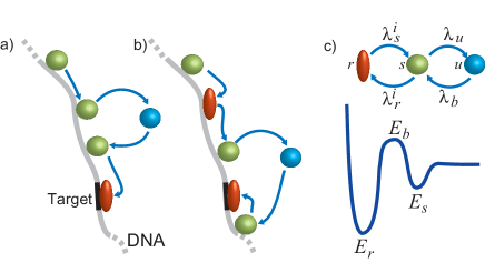
Figure 10: An illustration of the two-state model described in Sec. V. (a) A time sequence of a protein sliding in the $s$ mode (green circle), diffusing off the DNA (blue circle) and entering the target site in the $r$ mode (red oval). (b) A protein finding the target after entering the $r$ state. (c) An illustration of the rates and the energy landscape which governs them at each location, $i=1,...,N$, along the DNA. Here $\lambda_{r}^{i}\propto e^{-(E_{b}^{i}-E_{s}^{i})/k_{B}T}$, $\lambda_{s}^{i}\propto e^{-(E_{b}^{i}-E_{r}^{i})/k_{B}T}$ and $\lambda_{u}\propto e^{-E_{s}^{i}/k_{B}T}$, while $\lambda_{b}$ depends on details of the three-dimensional diffusion process.

Based on a quantitative analysis of this model, we argue that due to the occurrence of several time scales in the search process the widely used definition of the reaction rate of a single protein as the inverse of the average search time $t^{ave}$ HANGGI1990 , is generally irrelevant as a measure of the efficiency of target location on DNA. When $n_{p}$ proteins are searching for the target, the relevant quantity is the probability $\mathcal{R}_{n_{p}}(t)$ for a reaction to occur before time $t$. We show below that $\mathcal{R}_{n_{p}}(t)$ can reach values close to one on a time scale $t_{n_{p}}^{typ}$ which can be orders of magnitude smaller than the average search time, $t_{n_{p}}^{ave}$. Both the typical and the average search times can be orders of magnitude smaller than the naive approach based on a one time scale assumption which gives $t^{ave}/n_{p}$.

Our analysis has several important merits. First, it reports a fast search time despite a very strong binding of the protein in the recognition state to any site on the DNA. This renders the question of stability in the recognition state irrelevant. We suggest that within this model the measured binding energies of proteins to the DNA are irrelevant to the kinetics of the search process; the relevant quantities are transition rates (specified below). Second, we show that with a proper choice of parameters one may solve the speed-stability paradox without designing the target. We make two comments. (i) While there is no equilibrium stability within this model it will be shown that the protein is present on the target site for an extended period of time. (ii) Within this model the kinetics are independent of the equilibrium properties. Therefore, it is straightforward to add equilibrium stability within it.

The model consists of $n_{p}$ proteins which can each be in three states : (i) an unbound state, $u$, in which it performs three-dimensional diffusion (jumping), (ii) a search state, $s$, where it is weakly bound to the DNA, performing one-dimensional diffusion (sliding) and (iii) a recognition state, $r$, where it is tightly bound to the DNA. We assume, for simplicity, that in the recognition state the protein is trapped in a deep energy well (as justified by the experimentally measured strong binding energies) and is unable to move SM2004 . The transition rates, $\lambda_{s}^{i}$, $\lambda_{r}^{i}$, $\lambda_{b}$ and $\lambda_{u}$, between the different states are defined in Fig. 10. To model sliding, in the $s$ state the protein can move with transition rate $\lambda_{0}/2$ to neighboring sites on the DNA. Note that the transition rates $\lambda_{r}^{i}$ and $\lambda_{s}^{i}$ are expected in general to depend on the location $i=1\ldots N$ along the DNA. In principle $\lambda_{0}$ and $\lambda_{u}$ also have a dependence on $i$. As justified later this will have a weaker effect on our results and we omit it for clarity. Finally, after a jump we assume that the protein relocates to a random position on the DNA due to its packed conformation SK2009 .

The presentation of the model gives many details of the derivations of the results. However, we have made an effort to end each subsection with a highlight of the main results. Furthermore, some subsection focus only on results.

V.1 Non disordered case

To gain an understanding of the difference between the two time scales $t_{n_{p}}^{typ}$, $t_{n_{p}}^{ave}$  and the naive estimation $t^{ave}/n_{p}$ we first consider a single searcher, $n_{p}=1$, in a simplified model where the transition rates $\lambda_{r}^{i}=\lambda_{r}$ and $\lambda_{s}^{i}=\lambda_{s}$ are independent of $i$ except at the target site $\mathcal{T}$ (see Fig. 11$(a)$). The target site in this section is designed such that the transition rates on the target are different from the transition rates on the rest of DNA. At the target site the transition rate from the $s$ state to the $r$ state is denoted by $\lambda_{r}^{\mathcal{T}}$ and the transition rate from the $r$ state to the $s$ state is denoted by $\lambda_{s}^{\mathcal{T}}$ ($\lambda_{s}^{\mathcal{T}}$  is irrelevant for the calculation of the first-passage time properties). As stated above, in our considerations we analyze a process of search and recognition based only on a barrier discrimination and $P^{\cal T}=1/N$. Therefore, the relation

$$\frac{\lambda_{r}}{\lambda_{s}}=\frac{\lambda_{r}^{\mathcal{T}}}{\lambda_{s}^{\mathcal{T}}}$$ (48)

holds.

To analyze the model we first consider the probability

$$\mathcal{R}(t)=\int_{0}^{t}P(t^{\prime})dt^{\prime}$$ (49)

that the protein finds its target before time $t$, where $P(t)$ is the distribution of the first-passage time (FPT) R2001 to the target (we drop the subscript when $n_{p}=1$).

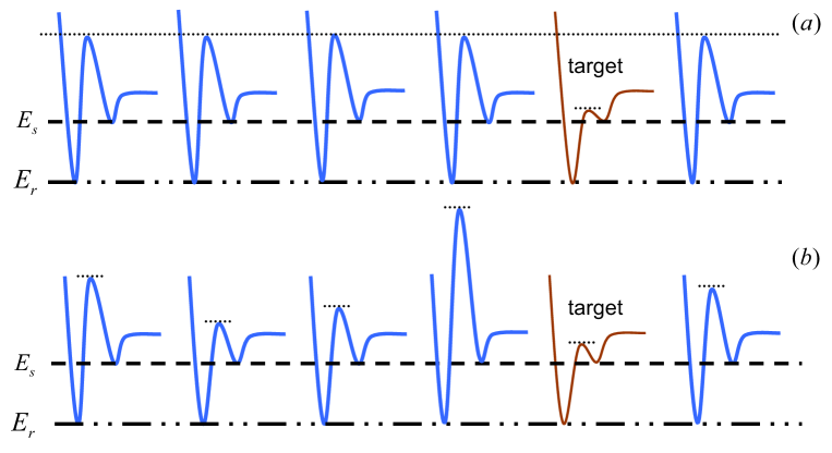
Figure 11: An illustration of the free energy landscape used in non-disordered and disordered models. (a) Each free energy profile represents a site on the DNA. All sites have the same profile except for the target that is designed to have smaller barrier. (b) Each free energy profile represents a site on the DNA. The energies of the $s$ and $r$ modes are fixed for all sites including the target. The barrier height is drawn from a Gaussian distribution while the target is defined as the site with the smallest barrier.

The Laplace transform,

$${\tilde{P}}(s)=\int_{0}^{\infty}e^{-st}P(t)dt,$$ (50)

of $P(t)$ can be obtained exactly. For simplicity we take a centered target site (labeled $0$). Consider, first, the joint probability density for a protein to find the target (in its $r$ state) at time $t=t_{s}+t_{r}$ starting from a location $x_{0}$ at $t=0$ before unbinding from the DNA. Here $t_{s}$ is the total time spent in the $s$ state and $t_{r}$ is the total time spent in the $r$ state. The probability that exactly $n$ transitions occurred from the $s$ state to the $r$ state is given by $\mathrm{\mathcal{P}}\left(n,\lambda_{r},t_{s}\right)$ where

$$\mathrm{\mathcal{P}}(n,\mu,t)=(\mu t)^{n}e^{-\mu t}/n!$$ (51)

is a Poisson distribution. The probability to spent a time $t_{r}$ in the $r$ state given that $n$ transitions occurred from the $s$ state to the $r$ state is $\lambda_{s}\mathrm{\mathcal{P}}\left(n-1,\lambda_{s},t_{r}\right)$ (with the convention $\mathrm{\mathcal{P}}(-1,\mu,t)\equiv\delta(t)/\mu$). The probability to stay on the DNA up to time $t=t_{s}+t_{r}$ starting at $t=0$ is given by $e^{-\lambda_{u}t_{s}}$. Finally, the probability to cross the barrier at the target at each visit of its $s$ state is given by

$$p_{1}=\frac{\lambda_{r}^{\mathcal{T}}}{1+\lambda_{u}/\lambda_{0}+\lambda_{r}^{\mathcal{T}}/\lambda_{0}}.$$ (52)

Therefore, the joint probability density for a protein to find the target at time $t=t_{s}+t_{r}$ starting from a location $x_{0}$ at $t=0$ before unbinding from the DNA is

$$P_{n}(t_{s},t_{r}|x_{0})=\lambda_{s}\mathrm{\mathcal{P}}\left(n-1,\lambda_{s},t_{r}\right)\mathrm{\mathcal{P}}\left(n,\lambda_{r},t_{s}\right)j_{p_{1}}\left(t_{s}|x_{0}\right)e^{-\lambda_{u}t_{s}},$$ (53)

where $j_{p_{1}}\left(t|x_{0}\right)$ is the FPT density at the target $x=0$ for a usual random walk starting from $x_{0}$ given that the probability to cross the barrier at the target at each visit in its $s$ state is $p_{1}$. The FPT density before unbinding starting from $x_{0}$ then reads:

$$J\left(t|x_{0}\right)=\sum_{n=0}^{\infty}\int_{0}^{\infty}\!\!\int_{0}^{\infty}\!\!dt_{s}dt_{r}\delta\left(t_{s}+t_{r}-t\right)P_{n}\left(t_{s},t_{r}|x_{0}\right).$$ (54)

After a Laplace transform and using

$${\tilde{\mathrm{\mathcal{P}}}}\left(n,\mu,s\right)=\frac{\mu^{n}}{\left(s+\mu\right)^{n+1}},$$ (55)

we find

$${\tilde{J}}\left(s|x_{0}\right)={\tilde{j}}_{p_{1}}\left(u\left(s\right)|x_{0}\right)$$ (56)

with

$$u(s)=\frac{s\left(s+\lambda_{r}+\lambda_{s}+\lambda_{u}\right)+\lambda_{s}\lambda_{u}}{s+\lambda_{s}}.$$ (57)

Following CBVM2004 ; pccp2008 we write the probability to find the target, $P\left(t\right)$ as

$$P\left(t\right)=\left\langle\sum_{m=0}^{\infty}\int_{0}^{\infty}dt_{m}{J}\left(t_{m}|x_{m}\right)\delta\left(t-\sum_{l=1}^{m-1}\left(t_{l}+\tau_{l}\right)-t_{m}\right)\underset{k=1}{\overset{m-1}{{\displaystyle\prod}}}dt_{k}d\tau_{k}\overline{{J}}\left(t_{k}|x_{k}\right)\lambda_{b}e^{-\lambda_{b}\tau_{k}}\right\rangle_{\left\{x_{k}\right\}}$$ (58)

where $\left\langle{}\right\rangle_{\left\{x_{k}\right\}}$ denotes an average over the DNA binding sites and $\overline{{J}}\left(t|x_{0}\right)$ is the probability to unbind before finding the $r$ state of the target starting from site $x_{0}$. This is given by

$$\overline{{J}}\left(t|x_{0}\right)=\lambda_{u}e^{-\lambda_{u}t}\left(1-\int_{0}^{t}dt^{\prime}J\left(t^{\prime}|x_{0}\right)e^{\lambda_{u}t^{\prime}}\right).$$ (59)

We assume that each DNA binding event occurs at a random position on the DNA. Thus

$$P\left(t\right)=\sum_{m=0}^{\infty}\int_{0}^{\infty}dt_{m}{J}\left(t_{m}\right)\delta\left(t-\sum_{l=1}^{m-1}\left(t_{l}+\tau_{l}\right)-t_{m}\right)\underset{k=1}{\overset{m-1}{{\displaystyle\prod}}}dt_{k}d\tau_{k}\overline{{J}}\left(t_{k}\right)\lambda_{b}e^{-\lambda_{b}\tau_{k}}$$ (60)

where ${J}\left(t\right)\equiv\left\langle{J}(t|x_{0})\right\rangle_{x_{0}}$ and $\overline{{J}}\left(t\right)\equiv\left\langle\overline{{J}}(t|x_{0})\right\rangle_{x_{0}}$. We then obtain the Laplace transformed FPT distribution as

$$\tilde{P}(s)={\tilde{J}}\left(s\right)\left[1-\frac{\lambda_{b}\lambda_{u}}{s+\lambda_{b}}\frac{1-{\tilde{J}}\left(s\right)}{u(s)}\right]^{-1}.$$ (61)

Using Eq. (56) and defining $\tilde{j}_{p_{1}}\left(s\right)\equiv\left\langle{\tilde{j}}_{p_{1}}\left(s|x_{0}\right)\right\rangle_{x_{0}}$ one obtains

$$\tilde{P}(s)=\tilde{j}_{p_{1}}\left(u\left(s\right)\right)\left[1-\frac{\lambda_{b}\lambda_{u}}{s+\lambda_{b}}\frac{1-\tilde{j}_{p_{1}}\left(u\left(s\right)\right)}{u\left(s\right)}\right]^{-1}.$$ (62)

Finally, $\tilde{j}_{p_{1}}\left(s\right)$ may be calculated using that

$$j_{p_{1}}\left(t\right) =\left\langle j_{p_{1}}\left(t|x_{0}\right)\right\rangle_{x_{0}}=\left\langle j\left(t|x_{0}\right)\right\rangle_{x_{0}}p_{1}+\left(1-p_{1}\right)\left\langle j\left(t|x_{0}\right)\right\rangle_{x_{0}}\ast j_{0}\left(t\right)p_{1}+$$ (63)

$$+\left(1-p_{1}\right)^{2}\left\langle j\left(t|x_{0}\right)\right\rangle_{x_{0}}\ast j_{0}\left(t\right)\ast j_{0}\left(t\right)p_{1}+...$$

where $j\left(t|x_{0}\right)$ is the FPT density at the target $x=0$ for a usual random walk starting from $x_{0}$ and ${j}_{0}\left(t\right)$ is the generating function of the first return time to site $0$ of a simple random walk. The $\ast$ symbol denotes a convolution. The Laplace transform of (63) gives

$$\tilde{j}_{p_{1}}\left(s\right)=\frac{p_{1}{\tilde{j}}\left(s\right)}{1-\left(1-p_{1}\right){\tilde{j}}_{0}\left(s\right)},$$ (64)

where

$$\tilde{j}(s)\equiv\left\langle\tilde{j}\left(s|x_{0}\right)\right\rangle_{x_{0}}\simeq\frac{1}{N}\sqrt{\frac{1+e^{-s/\lambda_{0}}}{1-e^{-s/\lambda_{0}}}}$$ (65)

and

$${\tilde{j}}_{0}\left(s\right)\simeq 1-\sqrt{1-e^{-2s/\lambda_{0}}}$$ (66)

for large $N$ montroll (see Appendix B for details).

Applying the Laplace transform to Eq. (49) and using Eq. (62) one obtains

$$\widetilde{\mathcal{R}}\left(s\right)=\frac{\tilde{P}(s)}{s}=\frac{\tilde{j}_{p_{1}}\left(u\left(s\right)\right)}{s}\left[1-\frac{\lambda_{b}\lambda_{u}}{s+\lambda_{b}}\frac{1-\tilde{j}_{p_{1}}\left(u\left(s\right)\right)}{u\left(s\right)}\right]^{-1}.$$ (67)

V.1.1 Large barrier regime

By analyzing the pole structure of Eq. (62) (see Appendix E) one can show that in the large barrier regime

$$\lambda_{s}\ll\lambda_{r}\ll\lambda_{u},\lambda_{b},\lambda_{0}$$ (68)

(with $\lambda_{u},\lambda_{b},\lambda_{0}$ of comparable order) the reaction probability simplifies to

$$\mathcal{R}\left(t\right)\simeq 1-qe^{-t/\tau_{1}}-\left(1-q\right)e^{-t/\tau_{2}}$$ (69)

with

$$q =\frac{1}{1+\frac{\lambda_{r}}{\lambda_{u}\kappa/N}},$$ (70)

$$\kappa =\frac{\sqrt{\coth\left(\frac{\lambda_{u}}{2\lambda_{0}}\right)}}{1+\frac{1-p_{1}}{p_{1}}\sqrt{1-e^{-2\lambda_{u}/\lambda_{0}}}},$$ (71)

$$\tau_{1} =\frac{1+\frac{\lambda_{u}}{\lambda_{b}}}{1+\frac{\lambda_{r}}{\lambda_{u}\kappa/N}}\frac{1}{\kappa\lambda_{u}/N}$$ (72)

and

$$\tau_{2}=\frac{1}{\lambda_{s}}\left(1+\frac{\lambda_{r}}{\lambda_{u}\kappa/N}\right).$$ (73)

Eq. (69) is a central result of this Section. We show below that a similar two exponents structure appears also in the disordered case. The short time scale $\tau_{1}$ characterizes searches where the protein never enters the $r$ state and is therefore independent of the binding energy $E_{r}$ (and hence of $\lambda_{s}$). The time scale $\tau_{2}$ characterizes searches where the protein enters the $r$ state, and is therefore much larger than $\tau_{1}$ in the case of strong binding ($\lambda_{s}$ small). In turn, $q$ is the probability of an event where the target is found without falling into a trap.

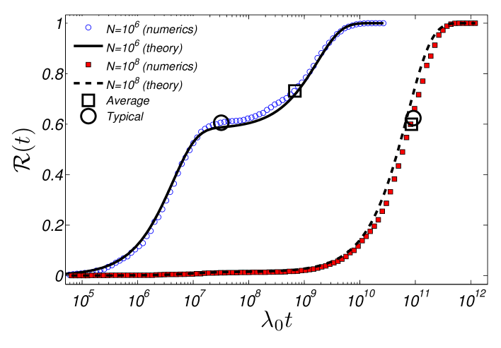
Figure 12: A plot of $\mathcal{R}(t)$ for $N=10^{6}$ (empty circles) and $N=10^{8}$ (filled squares) for non disordered case. Lines correspond to Eq. 69, with $\tau_{1}$, $\tau_{2}$ and $q$ derived analytically. Here $p_{1}=1$, $\lambda_{u}=10^{-2}\lambda_{0}$, $\lambda_{b}=0.1\lambda_{0}$, $\lambda_{r}=10^{-7}\lambda_{0}$ and $\lambda_{s}=10^{-9}\lambda_{0}$, in agreement with Wunderlich2009 . These correspond to energies, measured relative to the energy of the unbound state, of $E_{s}=-4.6k_{B}T$, $E_{b}=11.5k_{B}T$ and $E_{r}=-9.2k_{B}T$. The value of $p_{1}$ was taken to be one. Experiments suggest $\lambda_{0}\simeq 10^{6}\sec^{-1}$ for the Lac repressor WAC2006 .

Expression (69) enables an explicit determination of $t^{ave}=q\tau_{1}+(1-q)\tau_{2}$ and the typical search time $t^{typ}$. For convenience we define $t^{typ}$ through

$$\mathcal{R}\left(t^{typ}\right)={1-}\frac{1}{e},$$ (74)

i.e. the time after which the target is found with probability $1-1/e\simeq 0.63$ . The solution for Eq. (74) in the regime when the two time scales, $\tau_{1}$ and $\tau_{2}$ are well separated, $\tau_{1}\ll\tau_{2}$, is given by

$$t_{typ}=\left\{\begin{array}[]{cc}\tau_{1}\ln\frac{q}{\frac{1}{e}+q-1}&q>1-\frac{1}{e}\\ \tau_{2}\ln\frac{1-q}{\frac{1}{e}-q}&q<1-\frac{1}{e}\end{array}\right.$$ (75)

We stress that experimentally, the relevant time, where almost all search processes end, is $t^{typ}$ and not $t^{ave}$. In the regime $\lambda_{r}\gg\lambda_{u}\kappa/N$, one has $t^{typ}\simeq t^{ave}\simeq\tau_{2}$. A difference between $t^{typ}$ and $t^{ave}$ emerges as $\lambda_{r}$ is decreased and in the limit $\lambda_{r}\ll\lambda_{u}\kappa/N$ we find that $t^{typ}\simeq\tau_{1}/(2q-1)$ (with $q\simeq 1$) is independent of $\lambda_{s}$. This shows that for DNA lengths $N\leq\lambda_{u}\kappa/\lambda_{r}$, the typical search time is significantly smaller than the average even in the presence of deep traps ($\lambda_{s}$ small). This is a direct result of the competition between the two time scales.

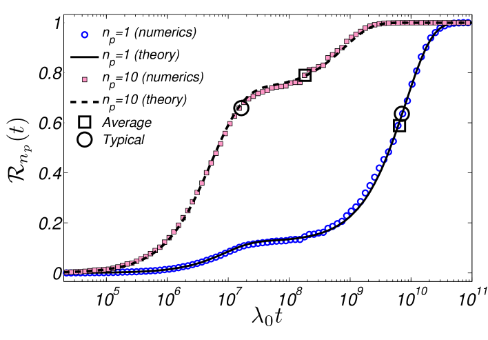
Figure 13: A plot of $\mathcal{R}_{n_{p}}(t)$ for $n_{p}=1$ (empty circles) and $n_{p}=10$ (filled squares) for non disordered case. Here $N=10^{6}$, $p_{1}=1$, $\lambda_{u}=10^{-4}\lambda_{0}$, $\lambda_{b}=0.1\lambda_{0}$, $\lambda_{r}=10^{-7}\lambda_{0}$ and $\lambda_{s}=10^{-9}\lambda_{0}$ (see Wunderlich2009 ). These correspond to energies, measured relative to the unbound state, of $E_{s}=-9.2k_{B}T$, $E_{b}=6.9k_{B}T$ and $E_{r}=-13.8k_{B}T$. The value of $p_{1}$ was taken to be one. Lines correspond to Eq. (69) with calculated values of $\tau_{1}$, $\tau_{2}$ and $q$. Note that here $\lambda_{u}$ is different from Fig. 12.

The results, compared with numerics which were performed using a standard continuous time Gillespie algorithm G1976 (see Appendix D for details), are shown in Fig. 12. We use realistic ranges of parameters (from available experimental data summarized in Wunderlich2009 ) which are specified in the caption. Since to the best of our knowledge there are no direct measurements of the barrier height for different DNA sequences, we assume this quantity to be of the same order of magnitude as the experimentally measured binding energies GMH2002 . It is found that $\mathcal{R}(t)$ reaches a plateau close to one on a typical time scale $t^{typ}$ which, for $N=10^{6}$, is smaller than the average search time $t^{ave}$ by two orders of magnitude. In next sections we show that results of this simple model may be applied to more realistic models.

V.2 Several searching proteins

The interesting regime $t^{typ}\ll t^{ave}$ requires a rather large barrier between the $s$ and $r$ state in the case of long DNA molecules (namely, $\lambda_{r}\leq\lambda_{u}\kappa/N$). One might argue that in general this condition may not be met by all proteins. Despite of this we now argue that this constraint can be, to a large extent, relaxed when $n_{p}$ proteins are searching for the target simultaneously. In this case even when for a single protein $t^{ave}\simeq t^{typ}$ the typical search time $t_{n_{p}}^{typ}$ of $n_{p}$ proteins can be significantly shorter than $t^{ave}/n_{p}$ even for relatively small values $n_{p}\approx 10-15$. Here, again, $t^{ave}$ is the average search time of a single protein and $t_{n_{p}}^{typ}$ is defined as in Eq. 74 where for $n_{p}$ proteins the first-passage distribution $P_{n_{p}}(t)$ is deduced from the cumulative distribution

$$\mathcal{R}_{n_{p}}(t)=1-\left(1-\mathcal{R}(t)\right)^{n_{p}}\;.$$ (76)

In Fig. 13 we show the results for $\mathcal{R}_{n_{p}}(t)$ for $n_{p}=10$. Note that as claimed above $t_{n_{p}}^{typ}\ll t^{ave}/n_{p}$, whereas $t^{typ}$ is close to $t^{ave}$ for one protein. This can be understood as follows. Using Eqs. (69) and (76), it is obvious that when $\tau_{2}\gg\tau_{1}$, the decay of $\mathcal{R}_{n_{p}}(t)$ is dominated by $\tau_{1}$ as long as $(1-q)^{n_{p}}\ll 1$. In essence since only one protein needs to find the target, the probability of a catastrophic event where the search time is of the order of $\tau_{2}$ is

$$p_{cat}=(1-q)^{n_{p}}$$ (77)

which decays exponentially fast with $n_{p}$. For large enough values of $n_{p}$ the short time scale $\tau_{1}$ controls the behavior of $\mathcal{R}_{n_{p}}(t)$, even if it is insignificant for the one protein search time. This implies that searches involving several proteins strongly suppress the long time-scales induced by the traps which control $t^{ave}$. In Section V.3 the average and typical search times are calculated for a given values of $\tau_{1}$, $\tau_{2}$, $q$ and $n_{p}$.

V.3 Calculating the average and typical search times

We showed above that the cumulative FPT distribution is given by

$$\mathcal{R}_{n_{p}}(t)=1-\left[qe^{-t/\tau_{1}}+\left(1-q\right)e^{-t/\tau_{2}}\right]^{n_{p}}$$ (78)

for the non-disordered model. In this section we calculate the typical and average search times for given values of $q$, $\tau_{1}$ and $\tau_{2}$. In the next section we discuss the disordered model in detail. As shown the disorder leaves the mathematical structure of the non-disordered case intact but with effective values of $q$, $\tau_{1}$ and $\tau_{2}$. Therefore all the results presented below and obtained for the non-disordered case can be easily extended to the disordered one.

V.3.1 Typical search time

When $\tau_{1}\ll\tau_{2}$, the typical search time $t_{n_{p}}^{typ}$, defined through

$$\mathcal{R}_{n_{p}}(t_{n_{p}}^{typ})={1-}\frac{1}{e}$$ (79)

can be obtained by assuming $t_{n_{p}}^{typ}\gg\tau_{1}$ or $t_{n_{p}}^{typ}\ll\tau_{2}$ and checking these assumptions self-consistently. Using this method we obtain for $n_{p}>1$

$$t_{n_{p}}^{typ}=\left\{\begin{array}[]{cc}\tau_{2}\left[\frac{1}{n_{p}}+\ln\left(1-q\right)\right]&{\rm for}\;\;\;n_{p}<\frac{1}{\ln\left(\frac{1}{1-q}\right)}\\ \tau_{1}\ln\frac{q}{e^{-1/n_{p}}+q-1}\simeq\frac{\tau_{1}}{qn_{p}}&{\rm for}\;\;\;n_{p}>\frac{1}{\ln\left(\frac{1}{1-q}\right)}\end{array}\right..$$ (80)

Therefore, for large enough $n_{p}$ it is widely independent of the binding energy in the $r$ mode.

V.3.2 Average search time

The average search time in the case of $n_{p}$ proteins is given by

$$t_{n_{p}}^{ave} =\int_{0}^{\infty}\left(1-\mathcal{R}(t)\right)^{n_{p}}dt=$$

$$=\overset{n_{p}}{\underset{n=0}{\sum}}\frac{n_{p}!}{\left(n_{p}-n\right)!n!}\frac{q^{n}\left(1-q\right)^{n_{p}-n}}{\frac{n}{\tau_{1}}+\frac{n_{p}-n}{\tau_{2}}}\;.$$ (81)

This sum may be estimated using a saddle point approximation. The saddle point is at $n^{\ast}=n_{p}q$ as expected (in the limit of a large $\frac{\tau_{2}}{\tau_{1}}$ ratio and using the Stirling approximation). Note that the saddle point approximation breaks when $n^{\ast}<1$. In this case the dominant term is $n^{\ast}=0$. When this is not the case we find

$$t_{n_{p}}^{ave}=\frac{\tau_{2}}{n_{p}}\left(1-q\right)^{n_{p}}+\frac{\tau_{1}}{n_{p}q}\frac{1}{1+\frac{\tau_{1}}{\tau_{2}}\frac{1-q}{q}}\;.$$ (82)

In the limit of $\tau_{1}\ll\tau_{2}$ the average time is given by

$$t_{n_{p}}^{ave}\simeq\left\{\begin{array}[]{cc}\frac{\tau_{2}}{n_{p}}\left(1-q\right)^{n_{p}}&{\rm for}\;\;\;n_{p}<\frac{\ln\frac{\tau_{2}}{\tau_{1}}}{\ln\left(\frac{1}{1-q}\right)}\\ \frac{\tau_{1}}{n_{p}q}&{\rm for}\;\;\;n_{p}>\frac{\ln\frac{\tau_{2}}{\tau_{1}}}{\ln\left(\frac{1}{1-q}\right)}\end{array}\right.$$ (83)

In Fig. 14 the average and typical search times are shown and compared to the approximations given by Eqs. (80) and (83). The data shown correspond to a choice of parameters where for $n_{p}=1$ the typical and average search times are roughly the same. Note that there is a large range of $n_{p}$ values for which $t_{n_{p}}^{typ}\ll t_{n_{p}}^{ave}$ and that they coincide again at very large values of $n_{p}$. The range of values of $n_{p}$ for which the typical and the mean search times differ scales as $\ln(\tau_{2}/\tau_{1})$. Remarkably, for small values of $n_{p}$ the average search time decreases faster than exponentially with the protein copy number.

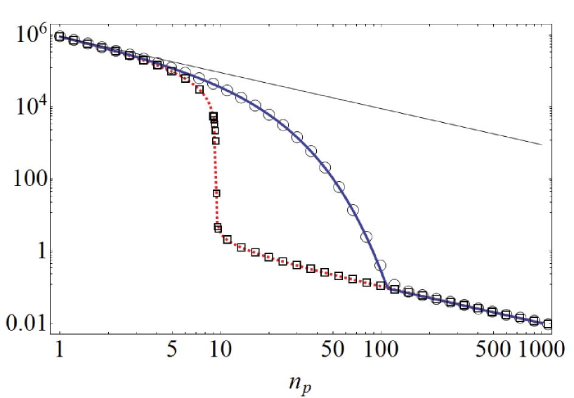
Figure 14: In this plot the average and the typical search times and their approximations are shown as a function of the number of proteins, $n_{p}$. Circles represent the average search time. Squares represent the typical search time, $t_{n_{p}}^{typ}$ (79). The blue, solid and thick line represents the approximation for the average time (83), the dashed red line represents the approximation for the typical search time (80) and the thin black line represents the naive estimate $\frac{t^{ave}}{n_{p}}$. Parameters chosen for this plot are $\tau_{1}=1$, $\tau_{2}=10^{6}$ and $q=0.1$.

V.4 Disordered case

In this section we study a disordered version of the model. Since the barrier plays a key role in the search we focus on effects of disorder in its height. To account for this we consider the case where the barrier height, $E_{b}^{i}$, is drawn from a Gaussian distribution:

$$p(E_{b}^{i})=\frac{e^{-\frac{(E_{b}^{i}-E_{0})^{2}}{2\sigma^{2}}}}{\sqrt{2\pi\sigma^{2}}}$$ (84)

such that the transition rate from the $s$ state to the $r$ state at site $i$ is given by

$$\lambda_{r}^{i}=\lambda_{0}\min\left(1,e^{-E_{b}^{i}}\right).$$ (85)

Introducing an energy difference between the $r$ state and the $s$ state (taken to be equal for all sites), $E_{r}$, the transition rate from the $r$ state to the $s$ state at site $i$ is given by

$$\lambda_{s}^{i}=\lambda_{0}e^{E_{r}}\min\left(1,e^{-E_{b}^{i}}\right)=\lambda_{r}^{i}e^{E_{r}}.$$ (86)

Similar to the affinity properties of the target site that is typically very close to the highest affinity among the non-target sites (see discussion above), we propose an intrinsic definition of the target as the site with the lowest barrier with no specifically designed properties (see Fig. 11(b)). Indeed, our previous assumption in Section V.1 that $\lambda_{r}^{\mathcal{T}}$ is large at the target site and $\lambda_{r}^{i}$ small everywhere else is a rather strong demand and corresponds to a designed target. Although we show below that the barrier discrimination mechanism may supply an efficient search even for the non-designed target, any special design of the target may significantly increase the search effectiveness. In the next subsection we analyze the disordered model using a mean-field approach and check the results using a numerical simulation in Section V.4.2.

V.4.1 Mean-field analysis

Within the mean-field approach we replace the different quantities by their disorder average and account for the barrier at the target site. We first compute the disorder averaged probability of crossing the barrier at the target at each visit. The probability density of the barrier height on the target site, $E_{b}^{\mathcal{T}}$, (the probability density of the minimal energy among $N$ normally distributed identical and independent random variables with a mean $E_{0}$ and variance $\sigma^{2}$) is HF2006

$$\Pr\left(E_{b}^{\mathcal{T}}\right)=\frac{d}{dE_{b}^{\mathcal{T}}}\left[\int_{-\infty}^{E_{b}^{\mathcal{T}}}\frac{e^{-\frac{\left(E-E_{0}\right)^{2}}{2\sigma^{2}}}}{\sqrt{2\pi}\sigma}dE\right]^{N}=-\frac{d}{dE_{b}^{\mathcal{T}}}\left[\frac{1}{2}\operatorname{erfc}\left(\frac{E_{b}^{\mathcal{T}}-E_{0}}{\sqrt{2}\sigma}\right)\right]^{N}.$$ (87)

For a given value of $E_{b}^{\mathcal{T}}$ the probability to pass over a barrier to the $r$ state is $\frac{e^{-E_{b}^{\mathcal{T}}}}{1+\lambda_{u}/\lambda_{0}+e^{-E_{b}^{\mathcal{T}}}}$. Thus the disorder averaged probability of crossing the barrier at the target at each visit is given by

$$\overline{p}_{1}=-\int_{-\infty}^{\infty}dE_{b}^{\mathcal{T}}\frac{e^{-E_{b}^{\mathcal{T}}}}{1+\lambda_{u}/\lambda_{0}+e^{-E_{b}^{\mathcal{T}}}}\frac{d}{dE_{b}^{\mathcal{T}}}\left[\frac{1}{2}\operatorname{erfc}\left(\frac{E_{b}^{\mathcal{T}}-E_{0}}{\sqrt{2}\sigma}\right)\right]^{N}.$$ (88)

Here we set the time scale of the activation process across the barrier to be $\lambda_{0}$. We finally assume that the expression for $u(s)$ of the non-disordered model (69) holds with $\lambda_{r}^{i}$ replaced by its average over the barrier energy. Using Eq. (85) this is given by

$${\bar{\lambda}}_{r}=\lambda_{0}\left[\int_{-\infty}^{0}\frac{e^{-\frac{\left(E_{b}-E_{0}\right)^{2}}{2\sigma^{2}}}}{\sqrt{2\pi}\sigma}dE_{b}+\int_{0}^{\infty}e^{-E_{b}}\frac{e^{-\frac{\left(E_{b}-E_{0}\right)^{2}}{2\sigma^{2}}}}{\sqrt{2\pi}\sigma}dE_{b}\right].$$ (89)

Also using Eq. (86), within the mean-field approximation $\lambda_{s}^{i}$ is replaced by

$$\overline{\lambda}_{s}={\bar{\lambda}}_{r}e^{E_{r}}$$ (90)

and $p_{1}$ replaced by $\overline{p}_{1}$. In the next Section we check these results numerically.

V.4.2 Numerical results and comparison to mean-field analysis

We now check the mean-field results using numerics. First, we show that the two scales scenario described above still holds. Indeed, Fig. 15 shows that $\mathcal{R}(t)$ is well fitted by Eq. (69) for realistic values of parameters. Note that in Figs. 15 and 16 we have chosen the worst scenario $E_{r}=-\infty$ so that $\lambda_{s}=0$ and the average search time and the value of $\tau_{2}$ are both infinite. This implies that for $n_{p}$ large enough the only relevant time scale is $\tau_{1}$ and the typical search time again takes the form $t_{n_{p}}^{typ}\simeq\frac{\tau_{1}}{qn_{p}}$ (the detailed calculation of the typical and average times is presented above in Section V.3). This enables a fast search even in the presence of very deep (even infinite) traps.

The regime of a fast search with $t_{n_{p}}^{typ}$ independent of the trap depth $E_{r}$ also requires, as above, a small catastrophe probability, $p_{cat}=\left(1-q\right)^{n_{p}}$ (see Eq. 77). We now show that this condition holds in a wide range of disorder parameters, $E_{0}$ and $\sigma$. To illustrate this, the dependencies (holding all other variables constant) of $p_{cat}$ and $t_{n_{p}}^{typ}$ on $\sigma$, obtained from numerics and the mean-field treatment, are shown in Fig. 16 for realistic values of parameters. Notably, the dependence of the catastrophe probability on the disorder strength is not monotonic so that the value of $p_{cat}$ can be minimized as a function of $\sigma$. This reflects the fact that for small values of $\sigma$ the DNA sequence has to be scanned many times before the target enters in the $r$ mode. Increasing $\sigma$ lowers the barrier at the target and therefore reduces the number of scans needed, which diminishes $p_{cat}$. For larger $\sigma$ the chance of falling into a trap increases due to lower secondary minima of the barrier, which leads to an increase of $p_{cat}$. As expected, $p_{cat}$ is dramatically decreased when $n_{p}$ is increased, even by a few units, and can remain small for a wide range of values of $\sigma$. For larger $\sigma$, $p_{cat}$ increases and $t_{n_{p}}^{typ}$ rises quickly as it starts to depend on $\tau_{2}$.

Summarizing and using the results of Section V.1, the mean-field approach predicts that in the high barrier regime $\overline{\lambda}_{s}\ll\overline{\lambda}_{r}\ll\lambda_{u},\lambda_{b},\lambda_{0}$ (with $\lambda_{u},\lambda_{b},\lambda_{0}$ of comparable order) the reaction probability simplifies to

$$\mathcal{R}(t)\simeq 1-qe^{-t/\tau_{1}}-(1-q)e^{-t/\tau_{2}}$$ (91)

with

$$q =\left(1+\frac{\overline{\lambda}_{r}}{\overline{\lambda}_{u}\kappa/N}\right)^{-1},$$ (92)

$$\kappa =\frac{\sqrt{\coth\left(\frac{\overline{\lambda}_{u}}{2\overline{\lambda}_{0}}\right)}}{1+\frac{1-\overline{p}_{1}}{\overline{p}_{1}}\sqrt{1-e^{-2\overline{\lambda}_{u}/\overline{\lambda}_{0}}}},$$ (93)

$$\tau_{1} =\frac{\overline{\lambda}_{b}+\overline{\lambda}_{u}}{\overline{\lambda}_{b}\left(\overline{\lambda}_{r}+\frac{\kappa\overline{\lambda}_{u}}{N}\right)}$$ (94)

and

$$\tau_{2}=\frac{\overline{\lambda}_{r}+\kappa\overline{\lambda}_{u}/N}{\overline{\lambda}_{s}\kappa\overline{\lambda}_{u}/N}.$$ (95)

In the case of a few proteins, searchers that fall into traps tend to occupy sites with low barriers and, therefore, increase the probability of other TFs to reach the target. Thus, Eq. (76), in which the searchers are assumed to be independent, provides a lower bound on the probability to reach the target. Here and below we assume that the number of proteins, $n_{p}$, is small enough (compared with $N$) such that this effect does not play a role and Eq. (76) is applicable.

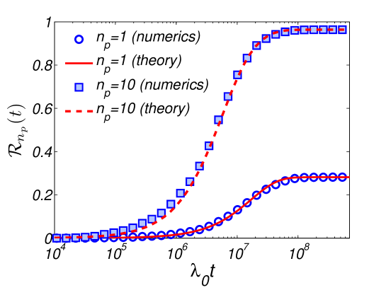
Figure 15: Plot of $\mathcal{R}_{n_{p}}(t)$ for $n_{p}=1$ (empty circles) and $n_{p}=10$ (filled squares) for the disordered model. The lines were obtained by fitting the form $1-(qe^{-t/\tau_{1}}+(1-q))^{{n}_{p}}$ to the numerical simulations with $q=0.2817$, $\lambda_{0}\tau_{1}=1.7\cdot 10^{7}$ and $\tau_{2}=\infty$. These are close to the mean field prediction $q=0.2827$, $\lambda_{0}\tau_{1}=1.1\cdot 10^{7}$. Here $\lambda_{u}=10^{-2}\lambda_{0}$ ($E_{s}=-4.6k_{B}T$), $\lambda_{b}=0.1\lambda_{0}$, $E_{0}=25.4k_{B}T$, $E_{r}=-\infty$ and $\sigma=5.3k_{B}T$. Note that here the average height of the barrier at the target site is $6.25k_{B}T$.

Most important, as advertised above, these results show that it is possible to obtain relatively small values of $t_{n_{p}}^{typ}$ and $p_{cat}$ with realistic values of the parameters (see Fig. 16). Reasonable search times (in the range of seconds) are obtained for a rather large range of $\sigma$ as long as $n_{p}$ is of the order of ten or more proteins suggesting another possible resolution of the speed and stability requirements. We stress that this mechanism can apply to any of the classes of TFs discussed above. This is a direct consequence of the decoupling of the stability and speed requirements. We note that by moderate changes in $E_{0}$ similar results can be obtained for much longer DNA sequences. In Appendix F we show that by increasing the disorder strength and the average barrier height such that

$$\frac{E_{0}}{\sigma}=\sqrt{2}\operatorname{erfc}^{-1}\left(\frac{2}{N}\right)\;,$$ (96)

a “perfect” searcher is obtained. By “perfect” it is implied that its search time is the same as a search on a flat (single state) model and that the target is reached with probability one.

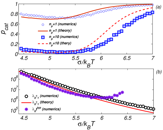
Figure 16: Results for the disordered model. Here $N=10^{6}$, $\lambda_{u}=10^{-2}\lambda_{0}$ ($E_{s}=-4.6k_{B}T$), $\lambda_{b}=0.1\lambda_{0}$, $E_{r}=-\infty$ and $E_{0}=25.4k_{B}T$. (a) $p_{cat}$ as a function of $\sigma$ for $n_{p}=1$ and $n_{p}=10$. (b) $t^{typ}$ for $n_{p}=10$ and $\tau_{1}$ are plotted as a function of $\sigma$. Using $\lambda_{0}=10^{6}\sec^{-1}$ WAC2006 for $n_{p}=10$ at the minimal $p_{cat}$ we find $t^{typ}\simeq 10sec$. Note that by moderate changes in $E_{0}$ similar results can be obtained for longer DNA sequences. The parameters for this plot are $\tau_{1}=1$, $\tau_{2}=10^{6}$, $q=0.1$.

VI Effective model and outcomes

As we showed in the previous section, by only using a barrier discrimination between different DNA sites a transcription factor may, in principle, serve as an efficient searcher and its complex with the target can be arbitrarily stable. Experiments show that different DNA sites are discriminated by their binding energy. Therefore, if a barrier mechanism is at work it is likely to be combined with an energetic discrimination between different sites.

Nonetheless, it is interesting to consider a scenario where there is only barrier discrimination. This could apply for TFs which have a very small target occupation probability $P^{\cal T}$. As we now show a barrier mechanism may lead to a high transient occupation probability of the target even with no energetic discrimination. When active processes are included the occupation probability can be made large even in the long-time limit. Furthermore, and in a more speculative manner, we show how the barrier mechanism can lead to a dynamical ordering of gene activation.

To show these we construct an effective model which uses the simple resulting mathematical structure of the previous section. Specifically, we use the cumulative probability

$$\mathcal{R}\left(t\right)=1-qe^{-\frac{t}{\tau_{1}}}-\left(1-q\right)e^{-\frac{t}{\tau_{2}}}.$$ (97)

In our discussion we concentrate on the target occupation probability. This fact and the simplicity of expression (97) allow one to describe our system using a three states model. Within this approach we only consider the $r$ state on the target ($\mathcal{T}$), the $r$ state off the target ($\mathcal{D}$) and one state for all other configurations (including $s$ states and the unbound state) ($\mathcal{U}$). The transition rates between the states are defined as follows: $\lambda^{\mathcal{D}}$ is the transition rate from $\mathcal{U}$ to $\mathcal{D}$, $\lambda_{-1}^{\mathcal{D}}$ is the transition rate from $\mathcal{D}$ to $\mathcal{U}$, $\lambda^{\mathcal{T}}$ is the transition rate from $\mathcal{U}$ to $\mathcal{T}$ and $\lambda_{-1}^{\mathcal{T}}$ is the transition rate from $\mathcal{T}$ to $\mathcal{U}$. The model is illustrated schematically in Fig. 17. As shown below, this simplification allows us to analyze the behavior of the system beyond its FPT properties.

Figure 17: Schematic representation of the three-states effective system. Here $\mathcal{T}$ denotes the $r$ state on the target, $\mathcal{D}$ denotes the $r$ state off the target and $\mathcal{U}$ denotes all other states (including the $s$ state and the unbound state).

To proceed we, first, show that the effective model yields the same cumulative FPT distribution $\mathcal{R}\left(t\right)$ as the original system. Specifically, it is straightforward to show that

$$\mathcal{R}(t)=1-\frac{\lambda^{+}-\lambda^{\mathcal{D}}}{\lambda^{+}-\lambda^{-}}e^{-t\lambda^{+}}-\frac{\lambda^{\mathcal{D}}-\lambda^{-}}{\lambda^{+}-\lambda^{-}}e^{-t\lambda^{-}},$$ (98)

where

$$\lambda^{\pm}=\frac{\lambda_{-1}^{\mathcal{D}}+\lambda^{\mathcal{D}}+\lambda^{\mathcal{T}}\pm\sqrt{(\lambda_{-1}^{\mathcal{D}}+\lambda^{\mathcal{D}}+\lambda^{\mathcal{T}})^{2}-4\lambda^{\mathcal{T}}\lambda_{-1}^{\mathcal{D}}}}{2}.$$ (99)

Comparing Eq. (69) with Eq. (98) one obtains relations between transition rates of the effective model and the full model:

$$\frac{\lambda^{+}-\lambda^{\mathcal{D}}}{\lambda^{+}-\lambda^{-}} =q$$

$$\lambda^{+} =\frac{1}{\tau_{1}}$$

$$\lambda^{-} =\frac{1}{\tau_{2}}.$$ (100)

The solution for the transition rates in the effective model are then

$$\lambda_{-1}^{\mathcal{D}} =\frac{\tau_{1}-q\tau_{1}+q\tau_{2}-\sqrt{\left(q\tau_{1}-\tau_{1}-q\tau_{2}\right)^{2}-4\tau_{1}\tau_{2}}}{2\tau_{1}\tau_{2}}\simeq\frac{1-q}{2\tau_{2}}$$

$$\lambda^{\mathcal{D}} =\frac{q\tau_{1}+\tau_{2}-q\tau_{2}}{\tau_{1}\tau_{2}}\simeq\frac{1-q}{\tau_{1}}$$

$$\lambda^{\mathcal{T}} =\frac{q\tau_{2}+\tau_{1}-q\tau_{1}+\sqrt{\left(q\tau_{1}-\tau_{1}-q\tau_{2}\right)^{2}-4\tau_{1}\tau_{2}}}{2\tau_{1}\tau_{2}}\simeq\frac{q}{\tau_{1}},$$ (101)

where we assumed a high barrier regime, $\tau_{2}\gg\tau_{1}$. Note that the transition rate from the target, $\lambda_{-1}^{\mathcal{T}}$, has no influence on the FPT properties. However, it determines properties of the target occupation probability in equilibrium. The time scale separation in the high barrier regime, $\tau_{1}\ll\tau_{2}$, implies

$$\lambda_{-1}^{\mathcal{D}}\ll\lambda^{\mathcal{D}}.$$ (102)

As stated above we consider a case where the binding energies of all sites (including the target) are the same so that in equilibrium the occupation probability of the target site is equal to the occupation probability of all other sites on the DNA. In this case, in equilibrium the occupation probability of the $\mathcal{D}$ state is $N$ times larger than the occupation probability of the $\mathcal{T}$ state. This implies within the simplified model that

$$\frac{\lambda^{\mathcal{D}}}{\lambda_{-1}^{\mathcal{D}}}=N\frac{\lambda^{\mathcal{T}}}{\lambda_{-1}^{\mathcal{T}}},$$ (103)

so that

$$\lambda_{-1}^{\mathcal{T}}=N\frac{\lambda_{-1}^{\mathcal{D}}\lambda^{\mathcal{T}}}{\lambda^{\mathcal{D}}}\simeq N\frac{q}{2\tau_{2}}.$$ (104)

Thus, we showed that a simple three-states effective model has the same dynamical and equilibrium properties as the original system. Below we use the effective model to analyze the search dynamics beyond FPT properties. For example, we consider equilibration dynamics, the possible existence of an active processes and temporal ordering in the activation/repression of multiple targets.

VI.1 Transient behavior

Following the above the occupation probability of the target site, $P^{\mathcal{T}}\left(t\right)$, evolves as

$$\frac{\partial P^{\mathcal{T}}}{\partial t} =\lambda^{\mathcal{T}}\left(1-P^{\mathcal{T}}-P^{\mathcal{D}}\right)-\lambda_{-1}^{\mathcal{T}}P^{\mathcal{T}}$$

$$\frac{\partial P^{\mathcal{D}}}{\partial t} =\lambda^{\mathcal{D}}\left(1-P^{\mathcal{T}}-P^{\mathcal{D}}\right)-\lambda_{-1}^{\mathcal{D}}P^{\mathcal{D}}$$

$$P^{\mathcal{U}} =1-P^{\mathcal{D}}-P^{\mathcal{T}}$$ (105)

where $P^{\mathcal{D}}\left(t\right)$ is the occupation probability of the $\mathcal{D}$ state, $P^{\mathcal{U}}\left(t\right)$ is the occupation probability of the $\mathcal{U}$ state and the initial conditions are $P^{\mathcal{U}}\left(t=0\right)=1$ so that $P^{\mathcal{T}}\left(t=0\right)=P^{\mathcal{D}}\left(t=0\right)=0$. These equations may be solved exactly. However, here we analyze the equations by noting that there are three time regimes. For $t\ll\frac{1}{\lambda^{\mathcal{T}}}$ the occupation probability of the target is close to its initial value, i.e. $P^{\mathcal{T}}\simeq 0$. For $\frac{1}{\lambda^{\mathcal{D}}}\gg t\gg\frac{1}{\lambda^{\mathcal{T}}}$ the protein equilibrated with the target but not with the rest DNA so that $P^{\mathcal{T}}\simeq\frac{1}{1+\frac{\lambda_{-1}^{\mathcal{T}}}{\lambda^{\mathcal{T}}}}$. Of course, this regime exist only when $\lambda^{\mathcal{T}}\gg\lambda^{\mathcal{D}}$. For $t\gg\frac{1}{\lambda^{\mathcal{D}}}$ the system reaches thermal equilibrium and the target occupation probability is given by $P^{\mathcal{T}}\simeq\frac{1}{1+\frac{\lambda^{\mathcal{T}}}{\lambda_{-1}^{\mathcal{T}}}\frac{\lambda_{-1}^{\mathcal{D}}}{\lambda^{\mathcal{D}}}}$. In Fig. 18 the occupation probability of the target site, $P^{\mathcal{T}}\left(t\right)$, is shown. Since there is no binding energy discrimination between DNA sites the occupation probability of the target in the long time limit is very small, $P^{\mathcal{T}}=\frac{1}{N}$. Note, however, that there is a transient regime where the occupation probability is large. In fact, in this regime the TF binds and unbinds many times from the target site before the system reaches thermal equilibrium.

The above discussion may be generalized to the case of a few proteins, $n_{p}>1$. In this case a mean-field generalization of (105) is

$$\frac{\partial n^{\mathcal{T}}}{\partial t} =\lambda^{\mathcal{T}}\left(n_{p}-n^{\mathcal{T}}-n^{\mathcal{D}}\right)\left(1-n^{\mathcal{T}}\right)-\lambda_{-1}^{\mathcal{T}}n^{\mathcal{T}}$$

$$\frac{\partial n^{\mathcal{D}}}{\partial t} =\lambda^{\mathcal{D}}\left(n_{p}-n^{\mathcal{T}}-P^{\mathcal{D}}\right)-\lambda_{-1}^{\mathcal{D}}n^{\mathcal{D}}$$

$$n^{\mathcal{U}} =n_{p}-n^{\mathcal{D}}-n^{\mathcal{T}}$$ (106)

with the initial conditions $n^{\mathcal{U}}\left(t=0\right)=n_{p}$ and $n_{\mathcal{T}}\left(t=0\right)=n^{\mathcal{D}}\left(t=0\right)=0$. Here $n^{\mathcal{T}},n^{\mathcal{D}}$ and $n^{\mathcal{U}}$ represent the mean-occupation number at the target in the ${\mathcal{T}}$, ${\mathcal{D}}$ and ${\mathcal{U}}$ respectively. The numerical solution of this nonlinear equation is shown in Fig. 18. The qualitative behavior is similar to the $n_{p}=1$ case: there are three time regimes. Using the same arguments as the $n_{p}=1$ case we find that, for $t\ll\frac{1}{\lambda^{\mathcal{T}}n_{p}}$ we have $n^{\mathcal{T}}\simeq 0$. For $\frac{1}{\lambda^{\mathcal{D}}}\gg t\gg\frac{1}{\lambda^{\mathcal{T}}n_{p}}$ we have $n^{\mathcal{T}}\simeq\frac{1}{1+\frac{1}{n_{p}}\frac{\lambda_{-1}^{\mathcal{T}}}{\lambda^{\mathcal{T}}}}$ and for $t\gg\frac{1}{\lambda^{\mathcal{D}}}$ the mean-occupation number is given by $n^{\mathcal{T}}\simeq\frac{1}{1+\frac{1}{n_{p}}\frac{\lambda^{\mathcal{T}}}{\lambda_{-1}^{\mathcal{T}}}\frac{\lambda_{-1}^{\mathcal{D}}}{\lambda^{\mathcal{D}}}}$. The intermediate regime, corresponding to a transient high occupation of the target, exist when $\lambda^{\mathcal{T}}n_{p}\gg\lambda^{\mathcal{D}}$. Its easy to check that for a large enough number of proteins, $n_{p}\gg\frac{\lambda^{\mathcal{D}}}{\lambda^{\mathcal{T}}}$, this regime exists even when $\lambda^{\mathcal{T}}<\lambda^{\mathcal{D}}$.

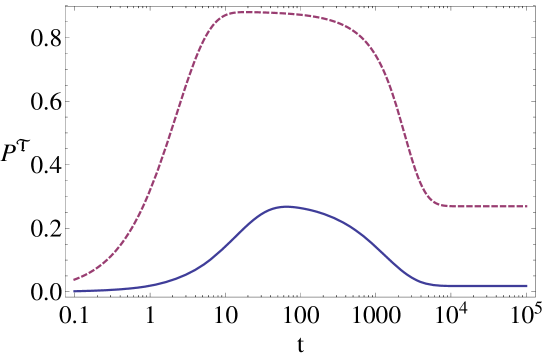
Figure 18: The occupation probability of the target site in the simplified model, $P^{\mathcal{T}}$, is show as a function of time. The parameters are $\lambda^{\mathcal{T}}=0.02$, $\lambda_{-1}^{\mathcal{T}}=0.05$, $\lambda^{\mathcal{D}}=10^{-3}$ and $\lambda_{-1}^{\mathcal{D}}=5\cdot 10^{-5}$. The blue solid (red dashed) line represents the $n_{p}=1$ ($n_{p}=20$) case.

Using this analysis we have shown that when the target site differs from the rest by a low barrier between the transcription factor’s $r$ and $s$ states its occupation has a transient nature. After a change in the environment, that activates the transcription factors, the occupation probability of the target increases exponentially with a fast time constant and after this decreases exponentially with a slow time constant to its final value. When the only discrimination between sites is the barrier height the final occupation probability of the target is very small, so that in the long time limit the system is in the same state as it was before the activation of the protein. By introducing a free energy binding energy discrimination between sites, the final occupation probability of the target may be significant such that the long time limit of the system may be different from the initial "pre-activated" state.

In general, when subjected to a change in the environmental condition, a cell typically responds by increasing the activity level of certain genes and decreasing the activity level of others. In many cases, the expression level of a certain gene changes temporarily, exhibiting a sharp increase or decrease, and later changing again, reaching a new steady-state (which often is similar the original state). This, two-step transient behavior, is widely observed in different transcriptional responses, from yeast Gasch2000 ; Braun2004 to human Ramoni2002 and may be explained by a negative feedback of an activated protein AlonBook . In this Section we showed how this kind of behavior naturally arises in a regulation system (composed of only one transcription factor) based on a barrier discrimination between distinct DNA sites.

VI.2 Steady-state and an existence of an active process

In equilibrium the occupation probability on a DNA site depends only on its binding energy. In cases where the only difference between the target and non-target sites is the barrier height between the $s$ and $r$ states, after the equilibration the probability to find the protein on the target site is very small. As we now show, by introducing an active process that returns the searcher to the initial state, $u$, with a transition rate, $\Omega$ (see Fig. 19) from any state, one may obtain a high occupation probability of the target site even at steady-state. This active process may be loosely thought of as cell division or degradation and production of the protein.

Figure 19: Schematic representation of the three-states effective system in presence of an active process $\Omega$.

In this case, for $n_{p}=1$ the equation for the occupation probabilities are given by

$$\frac{\partial P^{\mathcal{T}}}{\partial t} =\lambda^{\mathcal{T}}\left(1-P^{\mathcal{T}}-P^{\mathcal{D}}\right)-\left(\lambda_{-1}^{\mathcal{T}}+\Omega\right)P^{\mathcal{T}}$$

$$\frac{\partial P^{\mathcal{D}}}{\partial t} =\lambda^{\mathcal{D}}\left(1-P^{\mathcal{T}}-P^{\mathcal{D}}\right)-\left(\lambda_{-1}^{\mathcal{D}}+\Omega\right)P^{\mathcal{D}}.$$ (107)

In the steady-state ($\partial P^{\mathcal{T}}/\partial t=0$) the target site occupation probability is, therefore,

$$P^{\mathcal{T}}=\lambda^{\mathcal{T}}\frac{1+\frac{\lambda_{-1}^{\mathcal{D}}}{\Omega}}{\Omega+\frac{\lambda_{-1}^{\mathcal{T}}\lambda^{\mathcal{D}}+\lambda_{-1}^{\mathcal{D}}\left(\lambda^{\mathcal{T}}+\lambda_{-1}^{\mathcal{T}}\right)}{\Omega}+\left(\lambda^{\mathcal{D}}+\lambda_{-1}^{\mathcal{D}}+\lambda^{\mathcal{T}}+\lambda_{-1}^{\mathcal{T}}\right)}.$$ (108)

If in absence of an active process ($\Omega=0$) the steady-state occupation of the unbound state is small, the "on" rates, $\lambda^{\mathcal{D}}$ and $\lambda^{\mathcal{T}}$ are much larger than the "off" rates, $\lambda_{-1}^{\mathcal{D}}$ and $\lambda_{-1}^{\mathcal{T}}$. In this case one obtains three regimes depending on the value of $\Omega$

$$P^{\mathcal{T}}\simeq\left\{\begin{array}[]{cc}\frac{\lambda^{\mathcal{T}}}{\frac{\lambda_{-1}^{\mathcal{T}}\lambda^{\mathcal{D}}}{\lambda_{-1}^{\mathcal{D}}}+\lambda^{\mathcal{T}}+\lambda_{-1}^{\mathcal{T}}}&\Omega\ll\lambda_{-1}^{\mathcal{D}},\lambda_{-1}^{\mathcal{T}}\\ \frac{1}{1+\frac{\lambda^{\mathcal{D}}}{\lambda^{\mathcal{T}}}}&\lambda^{\mathcal{D}},\lambda^{\mathcal{T}}\gg\Omega\gg\lambda_{-1}^{\mathcal{D}},\lambda_{-1}^{\mathcal{T}}\\ \frac{\lambda^{\mathcal{T}}}{\Omega}&\Omega\gg\lambda^{\mathcal{D}},\lambda^{\mathcal{T}}\end{array}\right..$$ (109)

Note that in the second regime the occupation of the target site can by significant.

Similar to above, the approach can be generalized to several proteins (we use the same notation as in the previous subsection). When a few proteins act together the mean-field equations for the occupation probabilities are given by

$$\frac{\partial n^{\mathcal{T}}}{\partial t} =\lambda^{\mathcal{T}}\left(n_{p}-n^{\mathcal{T}}-n^{\mathcal{D}}\right)\left(1-n^{\mathcal{T}}\right)-\left(\lambda_{-1}^{\mathcal{T}}+\Omega\right)n^{\mathcal{T}}$$

$$\frac{\partial n^{\mathcal{D}}}{\partial t} =\lambda^{\mathcal{D}}\left(n_{p}-n^{\mathcal{T}}-n^{\mathcal{D}}\right)-\left(\lambda_{-1}^{\mathcal{D}}+\Omega\right)n^{\mathcal{D}}.$$ (110)

Here $n^{\mathcal{T}}$and $n^{\mathcal{D}}$ are the mean occupations numbers in the $\mathcal{T}$ and $\mathcal{D}$ state respectively. Assuming, as before, that without an active process the protein in equilibrium spends most of its time bound to the DNA we obtain in steady-state

$$n^{\mathcal{T}}\simeq\left\{\begin{array}[]{cc}\frac{\lambda^{\mathcal{T}}n_{p}}{\frac{\lambda_{-1}^{\mathcal{T}}\lambda^{\mathcal{D}}}{\lambda_{-1}^{\mathcal{D}}}+\lambda^{\mathcal{T}}n_{p}+\lambda_{-1}^{\mathcal{T}}}&\Omega\ll\lambda_{-1}^{\mathcal{D}},\lambda_{-1}^{\mathcal{T}}\\ \frac{1}{1+\frac{\lambda^{\mathcal{D}}}{\lambda^{\mathcal{T}}n_{p}}}&n_{p}\lambda^{\mathcal{D}},n_{p}\lambda^{\mathcal{T}}\gg\Omega\gg\lambda_{-1}^{\mathcal{D}},\lambda_{-1}^{\mathcal{T}}\\ \frac{\lambda^{\mathcal{T}}}{\Omega}n_{p}&\Omega\gg n_{p}\lambda^{\mathcal{D}},n_{p}\lambda^{\mathcal{T}}\end{array}\right..$$ (111)

The optimal $\Omega$ (that maximizes the steady-state occupation of the target, $n^{\mathcal{T}}$) is independent of $n_{p}$ and given by

$$\Omega_{opt}=\sqrt{\lambda_{-1}^{\mathcal{T}}\lambda^{\mathcal{D}}-\lambda_{-1}^{\mathcal{D}}\lambda^{\mathcal{D}}}-\lambda_{-1}^{\mathcal{D}}.$$ (112)

In Fig. 20 the steady-state probability of the target site as a function of the rate of the active process, $\Omega$, is shown.

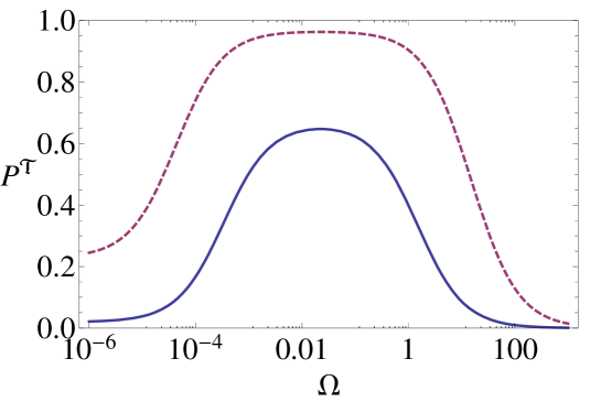
Figure 20: In this figure the occupation probability of the target site in the steady state is shown as a function of $\Omega$. The parameters are $\lambda^{\mathcal{T}}=1$, $\lambda_{-1}^{\mathcal{T}}=10^{-3}$, $\lambda^{\mathcal{D}}=0.5$ and $\lambda_{-1}^{\mathcal{D}}=10^{-5}$. The solid blue (dashed red) line represents the $n_{p}=1$ ($n_{p}=15$) case.

Summarizing, non-equilibrium effects of the barrier discrimination between DNA sites may lead to a high target occupation probability even at steady-state.

VI.3 The possibility of the genetic temporal ordering

It is often the case that each TF activates more than one gene A2007 . For example, in E. coli there are $68$ transcription factors which individually regulate more than $13$ operons RMC98 ; SMMA2002 . In some cases the activation of different genes, regulated by the same TF, are temporally ordered KMPSRLSA2001 ; RRSA2002 ; ZMRBSTSA2004 . In these systems it seems that the temporal ordering is not caused by the transcriptional network (for example, by a genetic cascade). It was suggested AlonBook ; GMH2002 that different genes have different activation thresholds. In this case a temporally increased concentration of the transcription factor activates them one-by-one. Different thresholds arise from non-linear effects, such as cooperativity between the transcription factors. Recently KWLGM2007 ; WM2008 ; BLV2008 it was proposed that genetic temporal ordering may be influenced by different distances between the production location of the TF and its target (this mechanism seems plausible only for prokaryotic cells).

Here we show that a search mechanism based on barrier discrimination can also lead to temporal ordering. This does not rely on cooperativity and appears even for a TF with a constant concentration. To show this we generalize the effective three states model to four states by adding an additional target site (see Fig. 21). Now the states of the model are the $r$ state of the first target ($\mathcal{T}_{1}$), the $r$ state of the second target ($\mathcal{T}_{2}$), the $r$ state out of both targets ($\mathcal{D}$) and the $\mathcal{U}$ states (including the $s$ states and the unbound state).

Figure 21: Schematic representation of the four-states effective system for temporal ordering. Here $\mathcal{T}_{1}$ denotes the $r$ state of the first target, $\mathcal{T}_{2}$ denotes the $r$ state of the second target, $\mathcal{D}$ denotes the $r$ state out of both targets and $\mathcal{U}$ denotes the remaining states (including the $s$ state and the unbound state).

For $n_{p}=1$ the evolution equations for the occupation probability of the first target, $P^{\mathcal{T}_{1}}$, the second target, $P^{\mathcal{T}_{2}}$, and the rest of the DNA, $P^{\mathcal{D}}$ are given by

$$\frac{\partial P^{\mathcal{T}_{1}}}{\partial t} =\lambda^{\mathcal{T}_{1}}\left(1-P^{\mathcal{T}_{1}}-P^{\mathcal{T}_{2}}-P^{\mathcal{D}}\right)-\lambda_{-1}^{\mathcal{T}_{1}}P^{\mathcal{T}_{1}}$$

$$\frac{\partial P^{\mathcal{T}_{2}}}{\partial t} =\lambda^{\mathcal{T}_{2}}\left(1-P^{\mathcal{T}_{1}}-P^{\mathcal{T}_{2}}-P^{\mathcal{D}}\right)-\lambda_{-1}^{\mathcal{T}_{2}}P^{\mathcal{T}_{2}}$$

$$\frac{\partial P^{\mathcal{D}}}{\partial t} =\lambda^{\mathcal{D}}\left(1-P^{\mathcal{T}_{1}}-P^{\mathcal{T}_{2}}-P^{\mathcal{D}}\right)-\lambda_{-1}^{\mathcal{D}}P^{\mathcal{D}}$$ (113)

while the occupation probability of the $\mathcal{U}$ state is determined by

$$P^{\mathcal{U}}=1-P^{\mathcal{T}_{1}}-P^{\mathcal{T}_{2}}-P^{\mathcal{D}}.$$ (114)

In the case of a few proteins the mean-field equations for the evolution of the occupation probability are

$$\frac{\partial n^{\mathcal{T}_{1}}}{\partial t} =\lambda^{\mathcal{T}_{1}}\left(n_{p}-n^{\mathcal{T}_{1}}-n^{\mathcal{T}_{2}}-n^{\mathcal{D}}\right)\left(1-n^{\mathcal{T}_{1}}\right)-\lambda_{-1}^{\mathcal{T}_{1}}n^{\mathcal{T}_{1}}$$

$$\frac{\partial n^{\mathcal{T}_{2}}}{\partial t} =\lambda^{\mathcal{T}_{2}}\left(n_{p}-n^{\mathcal{T}_{1}}-n^{\mathcal{T}_{2}}-n^{\mathcal{D}}\right)\left(1-n^{\mathcal{T}_{2}}\right)-\lambda_{-1}^{\mathcal{T}_{2}}n^{\mathcal{T}_{2}}$$

$$\frac{\partial n^{\mathcal{D}}}{\partial t} =\lambda^{\mathcal{D}}\left(n_{p}-n^{\mathcal{T}_{1}}-n^{\mathcal{T}_{2}}-n^{\mathcal{D}}\right)-\lambda_{-1}^{\mathcal{D}}n^{\mathcal{D}}$$ (115)

with

$$n^{\mathcal{U}}=n_{p}-n^{\mathcal{T}_{1}}-n^{\mathcal{T}_{2}}-n^{\mathcal{D}}.$$ (116)

Here $n^{\mathcal{U}},n^{\mathcal{T}_{1}},n^{\mathcal{T}_{2}}$ and $n^{\mathcal{D}}$ are the mean occupation numbers in the $\mathcal{U},\mathcal{T}_{1},\mathcal{T}_{2}$ and $\mathcal{D}$ states respectively. These equations may be solved analytically for the $n_{p}=1$ case and for the $n_{p}\gg 1$ case. In Fig. 22 one may see that by the tuning transition rates it is possible to obtain a temporal ordering of gene activation or/and repression for a single protein and few ($n_{p}=10$) proteins. Genes $\mathcal{T}_{1}$ and $\mathcal{T}_{2}$ are activated or repressed at different times depending on their association rates. The subsequent deactivation or/and repression of genes $\mathcal{T}_{1}$ and $\mathcal{T}_{2}$ take place if $\frac{\lambda^{\mathcal{T}_{1,2}}}{\lambda_{-1}^{\mathcal{T}_{1,2}}}\frac{\lambda_{-1}^{\mathcal{D}}}{\lambda^{\mathcal{D}}}\ll 1$ and occurs also at different times depending on their dissociation rates. This results, in principle, can be generalized to any number of genes.

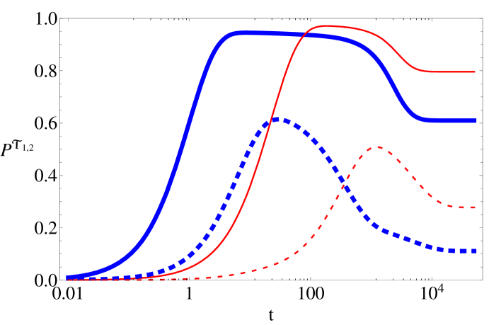
Figure 22: On this graph the occupation probabilities of two target sites, $P^{\mathcal{T}_{1}}$ (blue, thick lines) and $P^{\mathcal{T}_{2}}$ (red, thin lines), are shown as a function of time. The parameters are $\lambda^{\mathcal{T}_{1}}=0.05$, $\lambda_{-1}^{\mathcal{T}_{1}}=0.005$, $\lambda^{\mathcal{T}_{2}}=5\cdot 10^{-3}$, $\lambda_{-1}^{\mathcal{T}_{2}}=10^{-3}$, $\lambda^{\mathcal{D}}=10^{-3}$ and $\lambda_{-1}^{\mathcal{D}}=10^{-4}$. The solid (dashed) lines represent the $n_{p}=10$ ($n_{p}=1$) case.

VII Summary

Search and recognition problems appear in many contexts in biological systems. Organisms activate/repress many processes by specifically designed proteins. This may be an enzyme that catalyzes some chemical reaction by binding to specific molecules, a transcription factor that changes the transcriptional activity by binding to some specific locations on the DNA, etc. In fact, the flow of information, from a genotype to a phenotype and vice versa is regulated and implemented by searchers for specific DNA/RNA sequences. Needless to say, every particular biological searcher "invented" its own search strategy. However, there is hope that it is possible to divide all search strategies to a few classes similarly to the division of the transcription factors’ binding domains to a few DNA binding motifs Luscombe2000 . Different aspects of a transcription factor may dictate its strategy: the number of copies in the cell, its structure and function, its interactions with other proteins, the number of its targets and many more. The beginning of this review suggested a possible classification of TFs. It is certainly of great interest to extend it and test it on large databases. A particular simple classification arose when the length of the binding site of the protein to the DNA was considered.

The bulk part of the review deals with a possible scenario where TFs locate their target using barrier discrimination. This is different from other mechanisms which assume a local equilibration of the TF with its environment before the target is located. A more detailed discussion of those can be found in many other reviews HB89 ; HM2004 ; pccp2008 ; Mirny2009 ; kolo2010 ; rmp2011 . When assuming equilibration, each site on the DNA can be characterized by a single parameter - the binding energy at the site. According to the equilibrium assumption, this is the only parameter that may discriminate between different sites. On the contrary in the barrier model the search kinetics can become widely independent of the binding energy, and controlled by the barrier height. This gives a particularly simple resolution to the speed-stability paradox described in detail in this review. Moreover, it suggests that TFs can be weakly bound to the target site for extended period. We termed this transient activation. The end of the review dealt with more speculative processes that may occur in a barrier mechanism. These include time ordering in the activation of genes.

Under the conditions described above the search process in the barrier model is not characterized by a single time scale but by two. One short and one long. This leads to a distinction between typical search times, which are relevant to experiments, and average search times. The latter are dominated by rare events.

A clear indication that the barrier mechanism is at work in-vivo would lie in measurements of the full FPT distribution of a TF at a target gene, and the observation of more than one time scale. Even if the FPT distribution shows only a single time scale, the model predicts that the appearance of a new short time scale as $n_{p}$, number of searchers, is increased. Therefore, the appearance of the new time scale would be a clear indiction for the presence of the mechanism. In this case the typical search time will generally not scale as $1/n_{p}$. Such experimental data are not yet available but in principle accessible, and will hopefully provide in the near future a better understanding of the kinetics of gene activation.

Acknowledgments: We are grateful for many stimulating and critical discussions with E. Braun, A. Finkelstein, K. Keren and D. Levine.

Appendix A An information theoretic approach to the calculation of disorder parameters and binding energies

In Sections II we characterized the ability of a protein to recognize its target by the free energy gap between the target and the rest of the DNA sites and the equilibrium target occupation probability. As an alternative approach one often uses the information content of a protein, denoted by $IC$ SSGE86 ; HS99 . While our personal preference is to the presentation used in the main text the two can be used interchangeably. In this appendix we provide a brief overview of the relations between the information theory quantities (the information content and the sequence score) and the physical (the disorder strength and the binding energy of a sequence) quantities.

A.1 The information content and the disorder strength

Before turning to the information content of a protein of length $l_{p}$ we first discuss the information content associated with a single binding site $i$. Assuming that the frequency of each nucleotide in the genome is close to $1/4$ EcoliGenome , this quantity, denoted by $IC_{i}$, is given by its maximal amount of information minus its Shannon entropy. Note that we consider the $IC$ of the “specific” protein conformation. The non-specific one, presumably, does not contain any information. With this in mind we have

$$IC_{i}=-\log_{2}(1/4)+\underset{s=\left\{A,T,C,G\right\}}{\sum}\Pr\left(s,i\right)\log_{2}\Pr\left(s,i\right)$$ (117)

where $\Pr\left(s,i\right)$ is defined in Eq. (2). This quantity is maximal when only one nucleotide type can bind to site $i$. In this case $\Pr\left(s,i\right)=\delta_{s,s^{\prime}}$ so that $IC_{i}=2bits$. If two types of nucleotides can bind with equal probability ($\Pr\left(s,i\right)=\frac{1}{2}\delta_{s,s^{\prime}}+\frac{1}{2}\delta_{s,s^{\prime\prime}}$) the information content is reduced to one bit. In a case when each of the four types of nucleotides can bind with an equal probability of $\frac{1}{4}$ the information content is zero.

With these definitions the total information content of the protein is given by a sum of information contents of all protein binding sites:

$$IC=\underset{i=1}{\overset{l_{p}}{\sum}}IC_{i}.$$ (118)

To identify the target this has to be larger than $\log_{2}N$. Using Eqs. (1),(2) and (118) we obtain

$$IC =2l_{p}+\underset{\textbf{s}}{\sum}\frac{e^{-U\left(\textbf{s}\right)}}{\underset{\textbf{s}}{\sum}e^{-U\left(\textbf{s}\right)}}\log_{2}\frac{e^{-U\left(\textbf{s}\right)}}{\underset{\textbf{s}}{\sum}e^{-U\left(\textbf{s}\right)}}=$$

$$=2l_{p}-\underset{\textbf{s}}{\sum}\frac{\frac{U\left(\textbf{s}\right)}{\ln 2}e^{-U\left(\textbf{s}\right)}}{\underset{\textbf{s}}{\sum}e^{-U\left(\textbf{s}\right)}}-\log_{2}\underset{\textbf{s}}{\sum}e^{-U\left(\textbf{s}\right)}=$$

$$=2l_{p}-\left(1-\frac{\partial}{\partial\beta}\right)\left(\log_{2}\underset{\textbf{s}}{\sum}e^{-\beta U\left(\textbf{s}\right)}\right)_{\beta=1}.$$ (119)

Since, as we mentioned above, $U\left(\textbf{s}\right)$ behaves to a good approximation as a Gaussian random variable the information content is given by

$$IC=2l_{p}-\left(1-\frac{\partial}{\partial\beta}\right)\left\langle\log_{2}\underset{i=1}{\overset{4^{l_{p}}}{\sum}}e^{-\beta U_{i}}\right\rangle_{\beta=1}$$ (120)

where $\left\{U_{i}\right\}$ is a set of Gaussian random variables with a probability density

$$\Pr(U_{i})=\frac{e^{-\frac{U_{i}^{2}}{2\sigma_{U}^{2}}}}{\sqrt{2\pi\sigma_{U}^{2}}}$$ (121)

and the angular brackets denote an average over realizations of disorder. The expression $\left\langle\log_{2}\underset{i=1}{\overset{4^{l_{p}}}{\sum}}e^{-\beta U_{i}}\right\rangle$ is similar to the free energy of the Random Energy Model and in the limit of a long protein ($l_{p}\gg 1$) may be solved using ideas developed in D1981 . This gives

$$\left\langle\log_{2}\underset{i=1}{\overset{4^{l_{p}}}{\sum}}e^{-\beta U_{i}}\right\rangle=2l_{p}+\left\langle\log_{2}\frac{\underset{U_{\min}}{\overset{\infty}{\int}}e^{-\frac{U^{2}}{2\sigma_{U}^{2}}}e^{-\beta U}dU}{\underset{U_{\min}}{\overset{\infty}{\int}}e^{-\frac{U^{2}}{2\sigma_{U}^{2}}}dU}\right\rangle$$ (122)

where $U_{\min}$ is the minimal observed energy which is well approximated by

$$\underset{-\infty}{\overset{U_{\min}}{\int}}\frac{e^{-\frac{U^{2}}{2\sigma_{U}^{2}}}}{\sqrt{2\pi\sigma_{U}^{2}}}dU=\frac{1}{4^{l_{p}}}$$ (123)

or

$$U_{\min}=-\sigma_{U}\sqrt{2}\operatorname{erfc}^{-1}\left(\frac{2}{4^{l_{p}}}\right)\simeq-2\sigma_{U}\sqrt{l_{p}\ln 2}.$$ (124)

In the limit of a long protein one obtains

$$\left\langle\log_{2}\underset{i=1}{\overset{4^{l_{p}}}{\sum}}e^{-\beta U_{i}}\right\rangle=\left\{\begin{array}[]{cc}0&\sigma_{U}\geq 2\sqrt{l_{p}\ln 2}\\ 2l_{p}+\frac{\beta^{2}\sigma_{U}^{2}}{2\ln 2}&\sigma_{U}<2\sqrt{l_{p}\ln 2}\end{array}\right..$$ (125)

Using Eq. (120) the information content is finally given by

$$IC=\left\{\begin{array}[]{cc}2l_{p}&\sigma_{U}\geq 2\sqrt{l_{p}\ln 2}\\ \frac{\sigma_{U}^{2}}{2\ln 2}&\sigma_{U}<2\sqrt{l_{p}\ln 2}\end{array}\right..$$ (126)

Schneider et al. SSGE86 suggested, and showed for a few transcription factors, that the information content is just sufficient for the target to be distinguished from the rest of the genome. Specifically, with $N$ potential binders, where $N$ is twice the genome length ($N\simeq 10^{7}bp$ for E. coli), the amount of the information needed to distinguish a single binder is $\log_{2}N$. Therefore, we would expect

$$IC\gtrsim\log_{2}N$$ (127)

If this is not fulfilled one expects a wrong sequence to be incorrectly recognized. Comparing Eqs. (126) and (127) this translated to a condition on the length of the protein

$$l_{p}\gtrsim\frac{\log_{2}N}{2}$$ (128)

and

$$\sigma_{U}\gtrsim\sqrt{2\ln N}.$$ (129)

This is identical to results of the simple arguments presented in Sec. II. This condition is based on the assumption that the maximal information content per TF’s length is two bits. However, we find that the average information content per TF’s length is actually close to one bit. This fact increases the minimal protein’s length from $11$ to $22$ basepairs. Similar conclusion may be obtained from Fig. 8.

One can see that the condition for a broad line information content (128) and (129) are identical to the conditions for a marginally gapped target with a significant occupation probability (see Sec. II). In the limit of $N\rightarrow\infty$ both conditions represent the freezing point of the Random Energy Model D1981 . In Fig. 23 a histogram of the information content of several DNA-binding proteins is presented. Note that many proteins have significantly less information about the target than predicted by Eq. (127). This conclusion is independent of any assumption on the binding energy distribution. More detailed study which includes eukaryotic TFs and other databases was done in Ref. Wunderlich2009 . In this work authors found that for an eukaryotic TFs the problem of the not sufficient information content is much more severe.

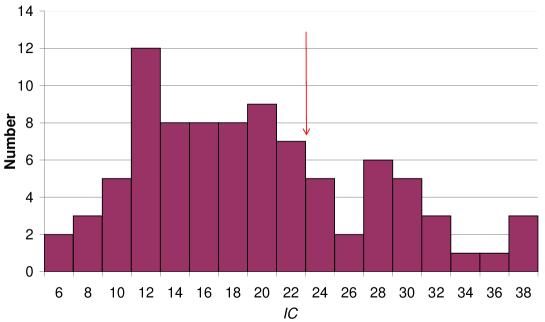
Figure 23: A histogram of the information content, $IC$. The data is based on the $89$ weight matrices of E. coli DNA-binding proteins from RegulonDB database regulonDB . The prediction of Eq. (127) is $23bits$ and is represented on the figure by the red arrow.

A.2 The sequence score and the binding energy

We showed above that the information content of many proteins is not sufficient for efficient target location. In Sec. II we present the same results, in particular, by comparing the binding energy of the target to the rest of the DNA. To this end we had to obtain the binding energy of a given sequence. In an information theory context this may be evaluated using a sequence score Staden1984 . The score of a sequence $\textbf{s}=\left(s_{1},s_{2},...,s_{l_{p}}\right)$ is defined as

$$Sc\left(\textbf{s}\right)=\underset{i=1}{\overset{l_{p}}{\sum}}\ln\left[4\Pr\left(s_{i},i\right)\right]=l_{p}\ln 4+\ln\left[\Pr\left(\textbf{s},i\right)\right]$$ (130)

where $\Pr\left(s_{i},i\right)$ is defined in Eq. (2) and

$$\Pr\left(\textbf{s},i\right)=\underset{i=1}{\overset{l_{p}}{{\displaystyle\prod}}}\Pr\left(s_{i},i\right).$$ (131)

The probability that a sequence s is bound is proportional to the Boltzmann factor $e^{-U\left(\textbf{s}\right)}$. Therefore, the binding energy, $U\left(\textbf{s}\right)$, is equal to the score of sequence s. Note that this convention differs from the one used in the text by a constant. The constant may be calculated by recalling that we defined the binding energy so that its average is zero. Therefore,

$$U\left(\textbf{s}\right) =-Sc\left(\textbf{s}\right)+l_{p}\ln 4+\frac{1}{4}\ln\left[\underset{i=1}{\overset{l_{p}}{{\displaystyle\prod}}}\underset{s_{i}^{\prime}=\left\{A,T,C,G\right\}}{{\displaystyle\prod}}\Pr\left(s_{i}^{\prime},i\right)\right]=$$

$$=-\underset{i=1}{\overset{l_{p}}{\sum}}\ln\frac{\Pr\left(s_{i},i\right)}{\sqrt[4]{\underset{s_{i}^{\prime}=\left\{A,T,C,G\right\}}{{\displaystyle\prod}}\Pr\left(s_{i}^{\prime},i\right)}}=\underset{i=1}{\overset{l_{p}}{\sum}}u_{i}\left(s_{i}\right).$$ (132)

where

$$u_{i}\left(s_{i}\right)=-\ln\frac{\Pr\left(s_{i},i\right)}{\sqrt[4]{\underset{s_{i}^{\prime}=\left\{A,T,C,G\right\}}{{\displaystyle\prod}}\Pr\left(s_{i}^{\prime},i\right)}}$$ (133)

is the contribution of site $i$ on the protein to the total binding energy of a sequence s. Eqs. (132,133) are used in Section II.2 to calculate (for each transcription factor) the binding energy of a given sequence.

Appendix B A derivation of Eqs. (65) and (66)

In this appendix we analyze the FPT properties of a simple random walk and derive Eqs. (65) and (66). A similar calculation can be found in Ref. montroll and is presented here for completeness. The Laplace transformed FPT probability density of the discrete space and continuum time random walk,

$$\widetilde{j}\left(x|x_{0};s\right)=\int_{0}^{\infty}e^{-st}j\left(x|x_{0};t\right)dt,$$ (134)

may be expressed in terms of the $z$-transformed FPT probability density of the discrete time random walk,

$$\widetilde{j}_{d}\left(x|x_{0};z\right)=\underset{t=1}{\overset{\infty}{\sum}}z^{t}j_{d}\left(x|x_{0};t\right),$$ (135)

by H95Volume1

$$\widetilde{j}\left(x|x_{0};s\right)=\widetilde{j}_{d}\left(x|x_{0};\frac{1}{1+s/\lambda_{0}}\right).$$ (136)

In discrete space and discrete time the occupation probability at origin starting from the site $x\geq 0$ at $t=0$ is given by

$$\widetilde{P}\left(x|x_{0};z\right)=\frac{\left(\frac{1-\sqrt{1-z^{2}}}{z}\right)^{\left|x-x_{0}\right|}}{\sqrt{1-z^{2}}}.$$ (137)

Using relation MW1965 that connects the FPT to the origin with the occupation probabilities

$$\widetilde{j}_{d}\left(x|x_{0};z\right)=\frac{\widetilde{P}\left(x|x_{0};z\right)-\delta_{x,x_{0}}}{\widetilde{P}\left(x|x;z\right)},$$ (138)

the $z$-transformed probability density of the first return time to site $0$ of a discrete time random walk is given by

$$\widetilde{j}_{d}\left(0|0;z\right)=1-\frac{1}{\widetilde{P}\left(0|0;z\right)}=1-\sqrt{1-z^{2}}$$ (139)

With Eq. (136) we obtain the Laplace transform of the first return time of a continuous time random walk (we denote this quantity in the text by ${\tilde{j}}_{0}\left(s\right)$)

$$\widetilde{j}\left(x|x_{0};s\right)=1-\sqrt{1-\left(\frac{1}{1+s/\lambda_{0}}\right)^{2}}\simeq 1-\sqrt{1-e^{-2s/\lambda_{0}}}.$$ (140)

The $z$-transformed probability density of the first-passage time to site $0$ from site $x$ of a discrete time random walk is given by

$$\widetilde{j}_{d}\left(0|x_{0};z\right)=\frac{\widetilde{P}\left(0|x_{0};z\right)}{\widetilde{P}\left(0|0;z\right)}=\left(\frac{1-\sqrt{1-z^{2}}}{z}\right)^{\left|x_{0}\right|}.$$ (141)

Its average over all possible starting sites in the large $N$ limit gives

$$\left\langle\widetilde{j}_{d}\left(0|x_{0};z\right)\right\rangle_{x_{0}}=\frac{1}{N}\underset{x_{0}=-N/2}{\overset{N/2}{\sum}}\left(\frac{1-\sqrt{1-z^{2}}}{z}\right)^{\left|x_{0}\right|}\simeq\frac{2}{N}\underset{x_{0}=1}{\overset{N/2}{\sum}}\left(\frac{1-\sqrt{1-z^{2}}}{z}\right)^{x_{0}}\simeq\frac{2}{N}\frac{1}{1-\frac{1-\sqrt{1-z^{2}}}{z}}\;.$$ (142)

Using Eq. (136) we obtain the Laplace transformed first passage time to site $0$ averaged over the initial sites of a discrete time random walk (we denote this quantity in the text by $\tilde{j}(s)\equiv\left\langle\tilde{j}\left(s|x_{0}\right)\right\rangle_{x_{0}}$)

$$\left\langle\widetilde{j}\left(0|x_{0};s\right)\right\rangle_{x_{0}}=\frac{2}{N}\frac{1}{1-\frac{1-\sqrt{1-\left(\frac{1}{1+s/\lambda_{0}}\right)^{2}}}{1+s/\lambda_{0}}}\simeq\frac{1}{N}\sqrt{\frac{1+e^{-s/\lambda_{0}}}{1-e^{-s/\lambda_{0}}}}.$$ (143)

Appendix C Specificity

The conditions discussed in Sec. IV B and Sec. IV C imply that

$$P_{d}\left(n_{p}=1\right)\ll e^{-\sigma_{U}^{2}}.$$ (144)

and

$$P^{{\cal\mathcal{T}}}\left(n_{p}=1\right)\gg P_{d}\left(n_{p}=1\right)$$ (145)

have to hold.

It is useful to separate the discussion into two cases.

Small disorder $\sigma_{U}\ll\sqrt{2\ln N}$

:

In this case

$$P^{{\cal\mathcal{T}}}\left(n_{p}=1\right)\simeq\frac{1}{1+Ne^{\sigma_{U}^{2}/2+U_{\mathcal{T}}}}$$ (146)

$$P_{d}\left(n_{p}=1\right)\simeq\frac{e^{\sigma_{U}\sqrt{2\ln N_{d}}}}{Ne^{\sigma_{U}^{2}/2}}\;,$$ (147)

so that the conditions (145) take the form

$$\sqrt{2\ln N}\gg\sigma_{U}\sqrt{1+\frac{2\sqrt{2\ln N_{d}}}{\sigma_{U}}}$$ (148)

$$U_{\mathcal{T}}\ll-\sigma_{U}\sqrt{2\ln N_{d}}.$$ (149)

Condition (148) can be satisfied for $2\sqrt{2\ln N_{d}}\ll\sigma_{U}\ll\sqrt{2\ln N}$ or for $\sigma_{U}\ll\min\left(\sqrt{2\ln N},2\sqrt{2\ln N_{d}},\frac{\ln N}{4\ln N_{d}}\right)$. The second condition (149) is satisfied automatically in the case of a non-designed TF (so that $U_{\mathcal{T}}=-\sigma_{U}\sqrt{2\ln N}$), in the case of designed TF with an additive binding energy (so that $U_{\mathcal{T}}=l_{p}E_{c}=-\sigma_{U}\sqrt{3l_{p}}$ where, as stated above, $l_{p}>\frac{2}{3}\ln N$) and, obviously, in the case of a gapped TF with cooperative binding energy (so that the value of $U_{\mathcal{T}}$ is not bound). Thus, in the small disorder regime the speed-stability paradox can be resolved by increasing the copy number of a TF without destroying the specificity. For a small number of dangerous sites, $N_{d}\ll N^{1/4}$, one may do so with a relatively large disorder while in the opposite case the upper bound on the disorder strength decreases. The number TF copies is given by

$$n_{p}\sim\max\left(e^{\sigma_{U}^{2}},Ne^{\sigma_{U}^{2}/2+U_{\mathcal{T}}}\right).$$ (150)

Large disorder $\sigma_{U}\gg\sqrt{2\ln N}$:

In this case

$$P^{{\cal\mathcal{T}}}\left(n_{p}=1\right)\simeq 1$$ (151)

$$P_{d}\left(n_{p}=1\right)=\frac{e^{\sigma_{U}\sqrt{2\ln N_{d}}}}{e^{\sigma_{U}\sqrt{2\ln N}}}.$$ (152)

so that the conditions (145) take the form

$$\frac{e^{\sigma_{U}\sqrt{2\ln N_{d}}}}{e^{\sigma_{U}\sqrt{2\ln N}}}\ll e^{-\sigma_{U}^{2}}$$ (153)

or

$$\sqrt{2\ln N}-\sqrt{2\ln N_{d}}\gg\sigma_{U}.$$ (154)

This condition cannot be satisfied simultaneously with the regime assumption $\sqrt{2\ln N}\ll\sigma_{U}$. Thus, in the large disorder regime the speed-stability paradox cannot be resolved by increasing the copy number of a TF without destroying the specificity.

Appendix D Details of the simulations

The model is simulated using a standard continuous time Gillespie algorithm G1976 . The protein on a given site, $i$, in the $s$ mode can perform four possible moves: it can move in one of the possible directions along the DNA with probability $\frac{\lambda_{0}/2}{\lambda_{0}+\lambda_{r}^{i}+\lambda_{u}}$, go to the $r$ mode with probability $\frac{\lambda_{r}^{i}}{\lambda_{0}+\lambda_{r}^{i}+\lambda_{u}}$ or dissociate from the DNA and reassociate on a randomly chosen site with probability $\frac{\lambda_{u}}{\lambda_{0}+\lambda_{r}^{i}+\lambda_{u}}$. In the first two cases time is advanced by an amount drawn from a Poisson distribution with an average of $\frac{1}{\lambda_{0}+\lambda_{r}^{i}+\lambda_{u}}$. When the protein dissociates, the time is advanced by first, drawing a time from a Poissonian distribution with an average time of $\frac{1}{\lambda_{0}+\lambda_{r}^{i}+\lambda_{u}}$, and adding to it a time, drawn from a Poissonian distribution with an average $\frac{1}{\lambda_{b}}$. This corresponds to the time needed for a relocation to a new site. The $r$ mode can transform only into the $s$ mode. The time for this step is drawn from a Poisson distribution with an average time $\frac{1}{\lambda_{s}}$.

Appendix E Pole structure analysis and derivation of Eq. (69)

In this appendix we show that Eq. (69) holds when there is a sufficient time scale separation in the problem. Following standard practice we perform the inverse Laplace transform by studying the poles of $\widetilde{\mathcal{R}}\left(s\right)$. In our case $\widetilde{\mathcal{R}}\left(s\right)$ has no poles in the region $\operatorname{Re}\left\{s\right\}>0$ of the complex plane so that

$$\mathcal{R}\left(t\right)=\frac{1}{2\pi i}\int_{-i\infty}^{i\infty}e^{st}\widetilde{\mathcal{R}}\left(s\right)ds=\underset{s_{i}\in poles}{\sum}e^{s_{i}t}\operatorname*{Res}\left[\widetilde{\mathcal{R}}\left(s\right),s_{i}\right].$$ (155)

As we showed above (see Eq. (67))

$$\widetilde{\mathcal{R}}(s)=\frac{\tilde{j}_{p_{1}}\left(u\left(s\right)\right)}{s}\left\{1-\frac{\lambda_{b}\lambda_{u}}{s+\lambda_{b}}\frac{1-\tilde{j}_{p_{1}}\left(u\left(s\right)\right)}{u\left(s\right)}\right\}^{-1},$$ (156)

where

$$u(s)=\frac{s\left(s+\lambda_{r}+\lambda_{s}+\lambda_{u}\right)+\lambda_{s}\lambda_{u}}{s+\lambda_{s}}.$$ (157)

and

$$\tilde{j}_{p_{1}}\left(s\right)=\frac{p_{1}{\tilde{j}}(s)}{1-(1-p_{1}){\tilde{j}}_{0}(s)},$$ (158)

where

$$\tilde{j}(s)\equiv\left\langle\tilde{j}(s|x)\right\rangle_{x}\simeq\frac{1}{N}\sqrt{\frac{1+e^{-s/\lambda_{0}}}{1-e^{-s/\lambda_{0}}}}$$ (159)

and

$${\tilde{j}}_{0}(s)=1-\sqrt{1-e^{-2s/\lambda_{0}}}$$ (160)

for large $N$ montroll . Finally, $p_{1}$ is probability of crossing the barrier at the target at each visit of its $s$ state,

$$p_{1}=\frac{\lambda_{r}^{\mathcal{T}}}{1+\lambda_{u}/\lambda_{0}+\lambda_{r}^{\mathcal{T}}/\lambda_{0}}.$$ (161)

The trivial pole of $\widetilde{\mathcal{R}}(s)$ is easily found (from Eq. (156)) to be

$$s_{0}=0$$ (162)

and its residue is

$$\mathrm{Res}_{0}=1.$$ (163)

Note that a pole in $\widetilde{j}_{p_{1}}\left(u\left(s\right)\right)$ would not lead to a pole in $\widetilde{\mathcal{R}}\left(s\right)$ due to the occurrence of $\widetilde{j}_{p_{1}}\left(u\left(s\right)\right)$ in the numerator and denominator. Thus, the equation for other poles is given by

$$\left(s+\lambda_{b}\right)u\left(s\right)=\lambda_{b}\lambda_{u}\left[1-\widetilde{j}_{p_{1}}\left(u\left(s\right)\right)\right].$$ (164)

Next we assume that $\lambda_{s}\ll\lambda_{r},\lambda_{u},\lambda_{b},\lambda_{0}$ with $\lambda_{u},\lambda_{b},\lambda_{0}$ of comparable order. The order of $\lambda_{r}$ will be discussed below in more details. We focus on the interesting regime $s/\lambda_{0}\ll 1$ in which the target is not found immediately. The analysis is carried out by considering the pole equation at different regimes. Using

$$\frac{u\left(s\right)}{\lambda_{0}}=\frac{1}{\lambda_{0}}\frac{s\left(s+\lambda_{r}+\lambda_{s}+\lambda_{u}\right)+\lambda_{s}\lambda_{u}}{s+\lambda_{s}}=\frac{s+\lambda_{r}+\lambda_{u}}{\lambda_{0}}-\frac{\lambda_{s}\lambda_{r}}{\lambda_{0}\left[\lambda_{s}-\left(-s\right)\right]}$$ (165)

and that $\left(-s\right)\ll\lambda_{0}$ and $\lambda_{r}\ll\lambda_{0}$ one may see that for

$$\left|\lambda_{s}-\left(-s\right)\right|\gg\frac{\lambda_{r}\lambda_{s}}{\lambda_{0}}$$ (166)

$\widetilde{j}\left(u\left(s\right)\right)\$is well approximated by $\frac{1}{N}\sqrt{\frac{1+e^{-\lambda_{u}/\lambda_{0}}}{1-e^{-\lambda_{u}/\lambda_{0}}}}$ and $\widetilde{j}_{0}\left(u\left(s\right)\right)\$is well approximated by $1-\sqrt{1-e^{-2\lambda_{u}/\lambda_{0}}}$. Below, for each solution we check the condition (166) to be self consistent.

Regime I: Here we consider $-s\gg\lambda_{s}$ so that to leading order $u\left(s\right)=s+\lambda_{r}+\lambda_{u}$ and

$$\widetilde{j}_{p_{1}}\left(u\left(s\right)\right) = \frac{p_{1}{\tilde{j}}(u\left(s\right))}{1-(1-p_{1}){\tilde{j}}_{0}(s)}\simeq$$

$$\simeq \frac{1}{N}\sqrt{\frac{1+e^{-\lambda_{u}/\lambda_{0}}}{1-e^{-\lambda_{u}/\lambda_{0}}}}\frac{1}{1+\frac{1-p_{1}}{p_{1}}\sqrt{1-e^{-2\lambda_{u}/\lambda_{0}}}}=\frac{1}{N}\frac{\sqrt{\coth\left(\frac{\lambda_{u}}{2\lambda_{0}}\right)}}{1+\frac{1-p_{1}}{p_{1}}\sqrt{1-e^{-2\lambda_{u}/\lambda_{0}}}}\equiv\frac{\kappa}{N}$$

in this regime (this is verified self-consistently below). Eq. (164) then reduces to

$$(s+\lambda_{b})\left(s+\lambda_{r}+\lambda_{u}\right)=\lambda_{b}\lambda_{u}\left(1-\frac{\kappa}{N}\right).$$ (167)

This equation has one pole of the order of $\lambda_{u},\lambda_{b}$, which corresponds to trajectories finding the target within the first sliding event. This pole can be discarded in the large $N$ limit since its residue scales as $1/N$. Its second pole reads, to leading order in $\lambda_{r}/\lambda_{u}$ and $1/N$:

$$\tau_{1}^{-1}\equiv-s_{1}\simeq\frac{\lambda_{b}\left(\lambda_{r}+\frac{\kappa\lambda_{u}}{N}\right)}{\lambda_{b}+\lambda_{u}}.$$ (168)

To ensure that $-s\gg\lambda_{s}$, as was assumed one should satisfy

$$\lambda_{s}\ll\frac{\lambda_{b}\left(\lambda_{r}+\frac{\kappa\lambda_{u}}{N}\right)}{\lambda_{b}+\lambda_{u}}.$$ (169)

The corresponding residue of $\widetilde{\mathcal{R}}\left(s\right)$ then reads:

$$\mathrm{Res}_{1}\simeq-q=-\frac{1}{1+\frac{\lambda_{r}}{\lambda_{u}\kappa/N}}.$$ (170)

This second pole corresponds to trajectories which find the target before crossing of the barrier. In the limit $\lambda_{r}\ll\frac{\kappa\lambda_{u}}{N}$, such events occur with a high probability $q\simeq 1$ and are characterized by a time scale $\tau_{1}\simeq\frac{N}{\kappa}\left(\frac{1}{\lambda_{b}}+\frac{1}{\lambda_{u}}\right)$. In the limit $\lambda_{r}\gg\frac{\kappa\lambda_{u}}{N}$ this second pole corresponds to processes which find the target before the typical time which characterizes a fall into the trap $\lambda_{r}{}^{-1}$ and without scanning the whole length. Such events are unlikely as shown by $q\ll 1$. To check the self-consistency we calculate the condition (166) for $s=s_{1}$.

$$\frac{\lambda_{b}\left(\lambda_{r}+\frac{\kappa\lambda_{u}}{N}\right)}{\lambda_{s}\left(\lambda_{b}+\lambda_{u}\right)}-1\gg\frac{\lambda_{r}}{\lambda_{0}}$$ (171)

but

$$\frac{\lambda_{b}\left(\lambda_{r}+\frac{\kappa\lambda_{u}}{N}\right)}{\lambda_{s}\left(\lambda_{b}+\lambda_{u}\right)}-1>\frac{\lambda_{r}}{\lambda_{s}}$$ (172)

so one may see that condition (166) for the first pole holds easily.

Regime II: Here we consider $-s\ll\lambda_{b}$. To proceed we take

$$\frac{p_{1}{\tilde{j}}(u\left(s\right))}{1-(1-p_{1}){\tilde{j}}_{0}(s)}\simeq\frac{1}{N}\sqrt{\frac{1+e^{-\lambda_{u}/\lambda_{0}}}{1-e^{-\lambda_{u}/\lambda_{0}}}}\frac{1}{1+\frac{1-p_{1}}{p_{1}}\sqrt{1-e^{-2\lambda_{u}/\lambda_{0}}}}=\frac{1}{N}\frac{\sqrt{\coth\left(\frac{\lambda_{u}}{2\lambda_{0}}\right)}}{1+\frac{1-p_{1}}{p_{1}}\sqrt{1-e^{-2\lambda_{u}/\lambda_{0}}}}\equiv\frac{\kappa}{N}$$ (173)

as before (this is verified self-consistently below). The equation becomes

$$s+\lambda_{s}+\lambda_{r}+\lambda_{u}=\lambda_{u}\left(s+\lambda_{s}\right)\left(1-\frac{\kappa}{N}\right).$$ (174)

The interesting pole is given by

$$\tau_{2}^{-1}\equiv-s_{2}\simeq\frac{\lambda_{s}\frac{\kappa\lambda_{u}}{N}}{\lambda_{r}+\frac{\kappa\lambda_{u}}{N}},$$ (175)

and the corresponding residue of $\widetilde{\mathcal{R}}\left(s\right)$ reads

$$\mathrm{Res}_{2}\simeq-\left(1-q\right)=-\left(1-\frac{1}{1+\frac{\lambda_{r}}{\lambda_{u}\kappa/N}}\right).$$ (176)

Similar to the case discussed above when $\lambda_{r}\gg\lambda_{u}\kappa/N$ the search involves a high chance of many entrances and exists from the $s$ state, as shown by $1-q\simeq 1$. In the opposite limit trajectories entering the $s$ state are very unlikely ($q\simeq 1$) and the search time is dominated by the trapping time $1/\lambda_{s}$. To check the self-consistency we calculate the condition (166) for $s=s_{2}$:

$$1-\frac{\frac{\kappa\lambda_{u}}{N}}{\lambda_{r}+\frac{\kappa\lambda_{u}}{N}}=1-\frac{1}{\frac{N\lambda_{r}}{\kappa\lambda_{u}}+1}\gg\frac{\lambda_{r}}{\lambda_{0}}$$ (177)

but

$$\frac{\kappa\lambda_{u}}{N}\ll\lambda_{0}\;.$$ (178)

This condition is also easily met. Applying the poles (162),(168), and (175) with the corresponding residues (163),(170), and (176) to Eq. (155) one obtains Eq. (69):

$$\mathcal{R}(t)\simeq 1-qe^{-t/\tau_{1}}-(1-q)e^{-t/\tau_{2}},$$ (179)

where

$$\kappa =\frac{\sqrt{\coth\left(\frac{\lambda_{u}}{2\lambda_{0}}\right)}}{1+\frac{1-p_{1}}{p_{1}}\sqrt{1-e^{-2\lambda_{u}/\lambda_{0}}}}$$

$$q =\frac{1}{1+\frac{\lambda_{r}}{\lambda_{u}\kappa/N}}$$

$$\tau_{1} =\frac{\lambda_{b}+\lambda_{u}}{\lambda_{b}\left(\lambda_{r}+\frac{\kappa\lambda_{u}}{N}\right)}$$

$$\tau_{2} =\frac{\lambda_{r}+\frac{\kappa\lambda_{u}}{N}}{\lambda_{s}\frac{\kappa\lambda_{u}}{N}}.$$ (180)

Appendix F Conditions for a perfect search

In this appendix we show that using the search and recognition strategy based on a disorder in a barrier height one may in principle achieve a "perfect" search without any design of the target and using only one searcher by optimizing the values of $E_{0}$ and $\sigma$. We define a "perfect" search as one where one searcher goes to the $r$ state of the target site with probability one ($q=1$) within a typical search time $t^{typ}\simeq\frac{N}{\sqrt{\lambda_{0}/\lambda_{u}}}\left(\frac{1}{\lambda_{u}}+\frac{1}{\lambda_{b}}\right)$. The last demand may be satisfied by ensuring that the barrier height on the target site, $E_{b}^{\mathcal{T}}$, is not positive with probability one. In this case the number of scans of the DNA that the searcher performs before a transition to the $r$ state is of order one. Below we show that this perfectly fast search can be achieved with a perfect recognition of the target, $q=1$. Namely we show that the occupation probability of the target in the infinite time limit may arbitrarily close to one. To this end we calculate below the occupation probability of each site on the DNA, $P_{i}$, and in particular, the occupation probability of the target site, $P^{\mathcal{T}}$. We take here $\lambda_{s}^{i}=0$ ($E_{r}=-\infty$) to ensure the stability of the protein-DNA complex after the target is located. We assume now (and check this assumptions self consistently) that $q=1$. This implies that the protein scans the whole DNA in the $s$ state (and, therefore, equilibrates in the $s$ states, but not in the $r$ state, on all DNA sites) before it passes over the barrier on the target. Thus, the transition rate to the $r$ state of site $i$ is given by $\frac{\lambda_{b}}{\lambda_{b}+\lambda_{u}}\lambda_{r}^{i}$. The time evolution of the occupation probability of the $r$ state at site $i$ is then given by

$$\frac{dP_{i}}{dt}=\frac{\lambda_{b}}{\lambda_{b}+\lambda_{u}}\lambda_{r}^{i}\left(1-\overset{N}{\underset{j=1}{\sum}}P_{j}\right).$$ (181)

At steady-state the occupation probability of the $r$ state at site $i$ is

$$P_{i}=\frac{\lambda_{r}^{i}/\lambda_{0}}{\overset{N}{\underset{j=1}{\sum}}\lambda_{r}^{i}/\lambda_{0}}.$$ (182)

The transition rate $\lambda_{r}^{i}$ is given by Eq. (85). As stated above, the barrier height, $E_{b}^{i}$, is drawn from a Gaussian distribution:

$$\Pr(E_{b}^{i})=\frac{e^{-\frac{\left(E_{b}^{i}-E_{0}\right)^{2}}{2\sigma^{2}}}}{\sqrt{2\pi\sigma^{2}}}.$$ (183)

The occupation probability of the site with the lowest barrier (a non-designed target) for a given realization of disorder is then given by

$$P^{\mathcal{T}}=\frac{e^{-E_{b}^{\mathcal{T}}}}{\overset{N}{\underset{i=1}{\sum}}e^{-E_{b}^{i}}}=\frac{1}{\overset{N}{\underset{i=1}{\sum}}e^{-E_{b}^{i}+E_{b}^{\mathcal{T}}}}=\frac{1}{1+\underset{i\neq\mathcal{T}}{\sum}e^{-E_{b}^{i}+E_{b}^{\mathcal{T}}}}$$ (184)

where $E_{b}^{\mathcal{T}}=\min\left\{E_{b}^{i}\right\}$ is the barrier height on the target site and the sum over $i\neq\mathcal{T}$ does not include the target site. Note that in the "thermodynamic" limit $N\rightarrow\infty$ and $\sigma\rightarrow\infty$ holding

$$\frac{\sigma}{\sqrt{2}\operatorname{erfc}^{-1}\left(\frac{2}{N}\right)}=const\equiv J,$$ (185)

where $\operatorname{erfc}^{-1}$ is the inverse complementary error function AS , this model is similar to the Random Energy Model and may be solved using the same approach D1981 .

The barrier height on the target site may be well estimated using

$$\int_{-\infty}^{E_{b}^{\mathcal{T}}}\frac{e^{-\frac{\left(E-E_{0}\right)^{2}}{2\sigma^{2}}}}{\sqrt{2\pi\sigma^{2}}}dE=\frac{1}{N}.$$ (186)

This gives

$$E_{b}^{\mathcal{T}}\simeq E_{0}-\sigma\sqrt{2}\operatorname{erfc}^{-1}\left(\frac{2}{N}\right),$$ (187)

As was mentioned above, we assume that for almost each realization of the disorder $E_{b}^{i}>0$ for every $i$. To make the search as fast as possible one should decrease the barrier of the target site. These two restrictions lead to the choice

$$E_{0}=\sigma\sqrt{2}\operatorname{erfc}^{-1}\left(\frac{2}{N}\right).$$ (188)

In this case $E_{b}^{\mathcal{T}}=0$ so that the probability distribution of the non-target sites may be well approximated in the large $N$ limit by

$$\Pr(E_{b}^{i\neq\mathcal{T}})=\left\{\begin{array}[]{cc}{\cal N}^{-1}e^{-\frac{\left(E_{b}^{i\neq\mathcal{T}}-E_{0}\right)^{2}}{2\sigma^{2}}}&E_{b}^{i\neq\mathcal{T}}>0\\ 0&E_{b}^{i\neq\mathcal{T}}<0\end{array}\right.,$$ (189)

where ${\cal N}$ is a normalization constant which can be easily obtained. Since for almost all realizations of the disorder the minimal barrier height is close to zero, Eq. (85) simplifies to

$$\frac{\lambda_{r}^{i}}{\lambda_{0}}=e^{-E_{b}^{i}}.$$ (190)

At steady-state the average occupation probability of the site with lowest barrier, $q$, is given by $\left\langle P^{\mathcal{T}}\right\rangle$. Using Eqs. (184), (190) with Jensen’s inequality,

$$\left\langle P^{\mathcal{T}}\right\rangle\geq\frac{1}{\left\langle\frac{1}{P^{\mathcal{T}}}\right\rangle},$$ (191)

one gets

$$q=\left\langle P^{\mathcal{T}}\right\rangle\gtrsim\frac{1}{\left\langle\frac{1}{P^{\mathcal{T}}}\right\rangle}\simeq\frac{1}{1+N\frac{\int_{0}^{\infty}e^{-\frac{\left(E-E_{0}\right)^{2}}{2\sigma^{2}}}e^{-E}dE}{\int_{0}^{\infty}e^{-\frac{\left(E-E_{0}\right)^{2}}{2\sigma^{2}}}dE}}=\left[1+N\frac{e^{-E_{0}+\frac{\sigma^{2}}{2}}\operatorname{erfc}\left(\frac{-E_{0}+\sigma^{2}}{\sqrt{2}\sigma}\right)}{1+\operatorname{erf}\left(\frac{E_{0}}{\sqrt{2}\sigma}\right)}\right]^{-1}.$$ (192)

Using Eqs. (185), (188) and taking the leading order in $\frac{1}{N}$ we obtain

$$q \gtrsim\left[1+\sqrt{2\pi\ln\left(\frac{N^{2}}{2\pi}\right)}\frac{\exp\left[\left(J-1\right)\left[\operatorname{erfc}^{-1}\left(\frac{2}{N}\right)\right]^{2}\right]\operatorname{erfc}\left[\left(J-1\right)\operatorname{erfc}^{-1}\left(\frac{2}{N}\right)\right]}{2}\right]^{-1}\simeq$$

$$\simeq\left\{\begin{array}[]{cc}\left[1+\frac{2}{J-1}\left(1-\frac{\ln\ln\frac{N^{2}}{2\pi}}{\ln\frac{N^{2}}{2\pi}}\right)^{-\frac{1}{2}}\right]^{-1}&J>1\\ \left[1+2\sqrt{2\pi\ln\frac{N^{2}}{2\pi}}e^{\left(J-1\right)^{2}\left[\operatorname{erfc}^{-1}\left(\frac{2}{N}\right)\right]^{2}}\right]^{-1}&J\leq 1.\end{array}\right.$$ (195)

In the limit $N\rightarrow\infty$ one gets a behavior similar to the usual second order phase transition of the Random Energy Model:

$$q=\left\{\begin{array}[]{cc}\frac{J-1}{J+1}&J\geq 1\\ 0&J<1\end{array}\right.$$ (196)

Therefore, for large enough $J$ the searcher finds its target with a probability close to one so that all our assumptions in this Section based on $q=1$ are self consistent. Also, since the typical barrier between the $s$ and $r$ states on the target is zero, the searcher finds its target within the facilitated diffusion limit. Note that, although the search and the recognition are perfect, the average time is infinite since there is a finite, $1-q$, probability to be trapped on a non-target site.

Summarizing, to ensure a perfect search one should set

$$\sigma=J\sqrt{2}\operatorname{erfc}^{-1}\left(\frac{2}{N}\right)$$ (197)

with some constant $J\gg 1$ and

$$E_{0}=\sigma\sqrt{2}\operatorname{erfc}^{-1}\left(\frac{2}{N}\right).$$ (198)

In this case the probability to find the target is

$$q=\frac{J-1}{J+1}\simeq 1-\frac{2}{J}$$ (199)

and the typical search time is comparable to the facilitated diffusion limit. Therefore, $J$ should be as large as possible. For the case of $n_{p}$ searchers (assuming that they are independent) the condition on $J$ becomes

$$p_{cat}=\left(1-q\right)^{n_{p}}=\left(\frac{2}{J+1}\right)^{n_{p}}\ll 1.$$ (200)

In fact, a perfect search may be impossible from practical reasons. For example, for $N=10^{6}$ our results suggest that to ensure $q=0.5$ one should take $E_{0}\simeq 67.7$ and $\sigma\simeq 14.3$. Such large energies may be difficult to achieve. Nevertheless, as we showed in Section V.4 the proposed mechanism of a barrier discrimination is very efficient even when parameters are far from perfect search conditions and the mean and the variance of the barrier energy are comparable to the mean and the variance of the experimentally found binding energy distribution.

References

- [1] J. J. Hopfield. Kinetic Proofreading: A New Mechanism for Reducing Errors in Biosynthetic Processes Requiring High Specificity. Proc. Nat. Acad. Sci. USA, 71(10):4135, 1974.
- [2] A. V. Hill. The combinations of haemoglobin with oxygen and with carbon monoxide. I. Biochem. J., 7(5):471, 1913.
- [3] A. Fersht. Enzyme structure and mechanism. W.H. Freeman, New York, San Francisco, 1985.
- [4] P. Schimmel and R. Alexander. All You Need Is RNA. Science, 281(5377):658, 1998.
- [5] T. R. Cech. The Ribosome Is a Ribozyme. Science, 289(5481):878, 2000.
- [6] A. Barzel and M. Kupiec. Finding a match: how do homologous sequences get together for recombination? Nature, 9:27, 2008.
- [7] C. Loverdo, O. Benichou, M. Moreau, and R. Voituriez. Enhanced reaction kinetics in biological cells. Nature Phys., 4:134, 2007.
- [8] P. Guptasarma. Does replication-induced transcription regulate synthesis of the myriad low copy number proteins of Escherichia coli? BioEssays, 17(11):987, 1995.
- [9] K. Robison, A. M. McGuire, and G. M. Church. A comprehensive library of DNA -binding site matrices for 55 proteins applied to the complete Escherichia coli k-12 genome. J. Mol. Biol., 284(2):241, 1998.
- [10] Y. Ishihama, T. Schmidt, J. Rappsilber, M. Mann, F. U. Hartl, M. Kerner, and D. Frishman. Protein abundance profiling of the Escherichia coli cytosol. BMC Genomics, 9(1):102, 2008.
- [11] Y. Taniguchi, P. J. Choi, G.-W. Li, H. Chen, M. Babu, J Hearn, A. Emili, and X. S. Xie. Quantifying E. coli Proteome and Transcriptome with Single-Molecule Sensitivity in Single Cells. Science, 329(5991):533, 2010.
- [12] K. Yamanaka and M. Inouye. Induction of CspA, an E. coli major cold-shock protein, upon nutritional upshift at 37°C. Genes to Cells, 6(4):279, 2001.
- [13] O. G. Berg, R. B. Winter, and P. H. von Hippel. Diffusion-driven mechanisms of protein translocation on nucleic acids. 1. models and theory. Biochem., 20(24):6929, 1981.
- [14] P. H. von Hippel and O. G. Berg. Facilitated target location in biological systems. J. Biol. Chem., 264(2):675, 1989.
- [15] S. E. Halford and J. F. Marko. How do site-specific DNA-binding proteins find their targets? Nucl. Acid. Res., 32(10):3040, 2004.
- [16] O. G. Berg and C. Blomberg. Association kinetics with coupled diffusional flows: Special application to the lac repressor-operator system. Biophys. Chem., 4:367, 1976.
- [17] R. B. Winter and P. H. Von Hippel. Diffusion-driven mechanisms of protein translocation on nucleid acids. 2. the Escherichia coli repressor-operator interaction : equilibrium measurements. Biochem., 20:6948, 1981.
- [18] R. B. Winter, O. G. Berg, and P. H. von Hippel. Diffusion-driven mechanisms of protein translocation on nucleic acids. 3. the Escherichia coli Lac repressor-operator interaction: Kinetic measurements and conclusions. Biochem., 20:6961, 1981.
- [19] A. Jeltsch, C. Wenz, F. Stahl, and A. Pingoud. Linear diffusion of the restriction endonuclease EcoRV on DNA is essential for the in vivo function of the enzyme. EMBO, 15(18):5104, 1996.
- [20] A. Jeltsch and A. Pingoud. Kinetic characterization of linear diffusion of the restriction endonuclease EcoRV on DNA . Biochem., 37(8):2160, 1998.
- [21] C. Bustamante, M. Guthold, X. Zhu, and G. Yang. Facilitated target location on DNA by individual Escherichia coli RNA polymerase molecules observed with the scanning force microscope operating in liquid. ASBMB, 274(24):16665, 1999.
- [22] N. Shimamoto. One-dimensional diffusion of proteins along DNA. J. Biol. Chem, 274(22):15293, 1999.
- [23] N.l P. Stanford, M. D. Szczelkun, J. F. Marko, and S. E. Halford. One- and three-dimensional pathways for proteins to reach specific DNA sites. EMBO, 19(23):6546, 2000.
- [24] J. Widom. Target site localization by site-specific, DNA -binding proteins. Proc. Natl. Acad. Sci. USA, 102(47):16909, 2005.
- [25] D. M. Gowers, G. G. Wilson, and S. E. Halford. Measurement of the contributions of 1d and 3d pathways to the translocation of a protein along DNA. Proc. Natl. Acad. Sci. USA, 102(44):15883, 2005.
- [26] Y. M. Wang, Robert H. Austin, and Edvard C. Cox. Single molecule measurement of repressor protein 1d diffusion on DNA. Phys. Rev. Lett., 97:048302, 2006.
- [27] J. Elf, G.-W. Li, and P. X. Xie. Probing transcription factor dynamics at the simple single-molecule level in a living cell. Science, 316:1191, 2007.
- [28] I. Bonnet, A. Biebricher, P.-L. Porte, C. Loverdo, O. Benichou, R. Voituriez, C. Escude, W. Wende, A. Pingoud, and P. Desbiolles. Sliding and jumping of single EcoRV restriction enzymes on non-cognate DNA. Nucl. Acid. Res., 36(12):4118, 2008.
- [29] P.-W. Fok, C.-L. Guo, and T. Chou. Charge-transport-mediated recruitment of DNA repair enzymes. J. Chem. Phys., 129(23):235101, 2008.
- [30] C. Loverdo, O. Benichou, R. Voituriez, A. Biebricher, I. Bonnet, and P. Desbiolles. Quantifying hopping and jumping in facilitated diffusion of DNA-binding proteins. Phys. Rev. Lett., 102(18):188101, 05 2009.
- [31] P.-W. Fok and T. Chou. Accelerated Search Kinetics Mediated by Redox Reactions of DNA Repair Enzymes. Biophys. J., 96:3949, 2009.
- [32] G Komazin-Meredith, R Mirchev, D E Golan, A M van Oijen, and D M Coen. Hopping of a processivity factor on DNA revealed by single-molecule assays of diffusion. Proc. Natl. Acad. Sci. USA, 105:10721, 2008.
- [33] G. Adam and M. Delbruck. Reduction of dimensionality in biological diffusion processes. In A. Rich and N. Davidson, editors, Structural Chemistry and Molecular Biology, pages 198–215, San Francisco, CA, 1968. Freeman.
- [34] D. R. Lesser, M. R. Kurpiewski, T. Waters, B. A. Connolly, and L. Jen-Jacobson. Facilitated distortion of the DNA site enhances EcoRI endonuclease-DNA recognition. Proc. Natl. Acad. Sci. USA, 90(16):7429, 1993.
- [35] U. Gerland, J. D. Moroz, and T. Hwa. Physical constraints and functional characteristics of transcription factor- DNA interaction. Proc. Natl. Acad. Sci. USA, 99(19):12015, 2002.
- [36] R. F. Bruinsma. Physics of protein-DNA interaction. Physica A, 313:211, 2002.
- [37] M. Slutsky and L. A. Mirny. Kinetics of protein-DNA interaction: Facilitated target location in sequence-dependent potential. Biophys. J., 87:4021, 2004.
- [38] M. Coppey, O. Benichou, R. Voituriez, and M. Moreau. Kinetics of target site localization of a protein on DNA: A stochastic approach. Biophys. J., 87:1640, 2004.
- [39] B. P. Belotserkovskii and D.A. Zarling. Analysis of a one-dimensional random walk with irreversible losses at each step: applications for protein movement on DNA. J. Theor. Biol., 226:195, 2004.
- [40] M. Kampmann. Facilitated diffusion in chromatin lattices: mechanistic diversity and regulatory potential. Mol. Microbiol., 57:889, 2005.
- [41] H. X. Zhou. A model for the mediation of processivity of DNA -targeting proteins by nonspecific binding: Dependence on DNA length and presence of obstacles. Biophysical Journal, 88:1608, 2005.
- [42] M. A. Lomholt, T. Ambjrnsson, and R. Metzler. Optimal target search on a fast-folding polymer chain with volume exchange. Phys. Rev. Lett., 95:260603, 2005.
- [43] T. Hu, A. Y. Grosberg, and B. I. Shklovskii. How proteins search for their specific sites on DNA: The role of DNA conformation. Biophys. J., 90:2731, 2006.
- [44] T. Hu and B. I. Shklovskii. How proteins search for their specific sites on DNA: The role of intersegment transfer. Phys. Rev. E, 76:051909, 2007.
- [45] G. Oshanin, H. S. Wio, K. Lindenberg, and S. F. Burlatsk. Intermittent random walks for an optimal search strategy: one-dimensional case. J. Phys., 19(6):065142, 2007.
- [46] I. Eliazar, T. Koren, and J. Klafter. Searching circular DNA strands. J. of Phys.: Cond. Matt., 19(6):065140, 2007.
- [47] A.G. Cherstvy, A.B.Kolomeisky, and A.A. Kornyshev. Protein-dna interactions: Reaching and recognizing the targets. J. Phys. Chem. B, 112:4741, 2008.
- [48] M. A. Lomholt, B. van den Broek, S. M. J. Kalisch, G. L. Wuiteand, and R. Metzler. Facilitated diffusion with DNA coiling. Proc. Natl. Acad. Sci. USA, 106:8204, 2009.
- [49] A.-M. Florescu and M. Joyeux. Description of nonspecific DNA-protein interaction and facilitated diffusion with a dynamical model. J. Chem. Phys., 130(1):015103, 2009.
- [50] A.-M. Florescu and M. Joyeux. Dynamical model of DNA-protein interaction: Effect of protein charge distribution and mechanical properties. J. Chem. Phys., 131(10):105102, 2009.
- [51] O. Givaty and Y. Levy. Protein sliding along DNA: Dynamics and structural characterization. J. Mol. Biol., 385:1087, 2009.
- [52] D. Vuzman and Y. Levy. DNA search efficiency is modulated by charge composition and distribution in the intrinsically disordered tail. Proc. Natl. Acad. Sci. USA, 107:21004, 2010.
- [53] D. Vuzman, M. Polonsky, and Y. Levy. Facilitated DNA search by multi-domain transcription factors: A cross-talk via a flexible linker. Biophys. J., 99:1202, 2010.
- [54] D. Vuzman, A. Azia, and Y. Levy. Searching DNA via a "monkey bar" mechanism: the significance of disordered tails. J. Mol. Biol., 396:674, 2010.
- [55] M. A. Díaz de La Rosa, E. F. Koslover, P. J. Mulligan, and A. J. Spakowitz. Dynamic Strategies for Target-Site Search by DNA-Binding Proteins. Biophys. J., 98:2943, 2010.
- [56] O. Benichou, C. Chevalier, B. Meyer, and R. Voituriez. Facilitated diffusion of proteins on chromatin. Phys. Rev. Lett., 106:038102, 2011.
- [57] A. B. Kolomeisky. Physics of protein-DNA interactions: Mechanisms of facilitated target search. Phys. Chem. Chem. Phys., 13:2088, 2011.
- [58] G. Tkačik and W. Bialek. Diffusion, dimensionality, and noise in transcriptional regulation. Phys. Rev. E, 79(5):051901, 2009.
- [59] Z. Tamari, N. Barkai, and I. Fouxon. Physical aspects of precision in genetic regulation. J. Biol. Phys., 37:213, 2011.
- [60] P. H. von Hippel and O. G. Berg. On the specificity of DNA-protein interactions. Proc. Nat. Acad. Sci. USA, 83(6):1608, 1986.
- [61] A. Jeltsch, J. Alves, H. Wolfes, G. Maass, and A. Pingoud. Pausing of the restriction endonuclease EcoRI during linear diffusion on DNA. Biochem., 33(34):10215, 1994.
- [62] O. Benichou, C. Loverdo, M. Moreau, and R. Voituriez. Optimizing intermittent reaction paths. Phys. Chem. Chem. Phys., 10:7059, 2008.
- [63] L. Mirny, M. Slutsky, Z. Wunderlich, A. Tafvizi, J. Leith, and A. Kosmrlj. How a protein searches for its site on DNA: the mechanism of facilitated diffusion. J. Phys. A, 42(43):434013, 2009.
- [64] R.K. Das and A.B.Kolomeisky. Facilitated search of proteins on DNA: Correlations are important. Phys. Chem.-Chem. Phys., 12:2999, 2010.
- [65] O. Benichou, C. Loverdo, M. Moreau, and R. Voituriez. Intermittent search strategies. Rev. Mod. Phys, 83:81, 2011.
- [66] Z. Wunderlich and L. A. Mirny. Different gene regulation strategies revealed by analysis of binding motifs. Trends in Genetics, 25:434, 2009.
- [67] O. Bénichou, Y. Kafri, M. Sheinman, and R. Voituriez. Searching fast for a target on DNA without falling to traps. Phys. Rev. Lett., 103:138102, 2009.
- [68] G.D. Stormo and D.S. Field. Specificity, free energy and information content in proteinDNA interactions. Trends Biochem. Sci., 23(178), 1998.
- [69] S.J. Maerkl and S.R. Quake. A systems approach to measuring the binding energy landscapes of transcription factors. Science, 315:233, 2007.
- [70] H. Herzel, E.N. Trifonov, O. Weiss, and I. Grosse. Interpreting correlations in biosequences. Physica A, 249:449, 1998.
- [71] C.-K. Peng, S. V. Buldyrev, A. L. Goldberger, S. Havlin, F. Sciortino, M.Simons, and H. E. Stanley. Long-range correlations in DNA sequences. Nature, 356:168, 1992.
- [72] G. D. Stormo, T. D. Schneider, and L. Gold. Quantitative analysis of the relationship between nucleotide sequence and functional activity. Nucl. Acid. Res., 14(16):6661, 1986.
- [73] M.O. Zhang and T.G. Marr. A weight array method for splicing signal analysis. Computer applications in the biosciences : CABIOS, 9(5):499, 1993.
- [74] M P Ponomarenko, J V Ponomarenko, A S Frolov, O A Podkolodnaya, D G Vorobyev, N A Kolchanov, and G C Overton. Oligonucleotide frequency matrices addressed to recognizing functional DNA sites. Bioinformatics, 15(7):631, 1999.
- [75] M. L. Bulyk, P. L. F. Johnson, and G. M. Church. Nucleotides of transcription factor binding sites exert interdependent effects on the binding affinities of transcription factors. Nucl. Acid. Res., 30(5):1255, 2002.
- [76] L. de Haan and A. Ferreira. Extreme Value Theory: An Introduction. Springer, 2006.
- [77] B. Derrida. Random-energy model: Limit of a family of disordered models. Phys. Rev. Lett., 45(2):79, 1980.
- [78] S. Gama-Castro, V. J. Jacinto, M. Peralta-Gil, A. Santos-Zavaleta, M. I. Penaloza-Spindola, B. Contreras-Moreira, J. Segura-Salazar, L. Muniz-Rascado, I. Martinez-Flores, H. Salgado, C. Bonavides-Martinez, C. Abreu-Goodger, C. Rodriguez-Penagos, J. Miranda-Rios, E. Morett, E. Merino, A. M.Huerta, and J. Collado-Vides. Regulondb (version 6.0): gene regulation model of Escherichia coli K-12 beyond transcription, active (experimental) annotated promoters and textpresso navigation. Nucl. Acid. Res., 36:D120, 2008.
- [79] S. Redner. A guide to first-passage process. Cambridge university press, Cambridge, UK, 2001.
- [80] S. Condamin, O. Benichou, V. Tejedor, R. Voituriez, and J. Klafter. First-passage times in complex scale-invariant media. Nature, 450:77, 2007.
- [81] O. Bénichou, C. Chevalier, J. Klafter, B. Meyer, and R. Voituriez. Geometry-controlled kinetics. Nature Chem., 2(6):472, 2010.
- [82] A. D. Riggs, H. Suzuki, and S. Bourgeois. Lac repressor-operator interaction I. equilibrium studies. J. Mol. Biol., 48(1):67, 1970.
- [83] A. D. Riggs, S. Bourgeois, and M. Cohn. The Lac repressor-operator interaction. 3. kinetic studies. J Mol Biol., 53(3):401, 1970.
- [84] M. von Smoluchowski. Mathematical theory of the kinetics of the coagulation of colloidal solutions. Z. Phys. Chem., 92:129, 1917.
- [85] M. B. Elowitz, M. G. Surette, P. E. Wolf, J. B. Stock, and S. Leibler. Protein mobility in the cytoplasm of Escherichia coli. J. Bacteriol., 181(1):197, 1999.
- [86] S. Y. Lin and A. D. Riggs. Lac repressor binding to non-operator DNA: detailed studies and a comparison of eequilibrium and rate competition methods. J. Mol. Biol., 72(3):671, 1972.
- [87] B. J. Terry, W. E. Jack, and P. Modrich. Facilitated diffusion during catalysis by EcoRI endonuclease. Nonspecific interactions in EcoRI catalysis. J. Biol. Chem., 260(24):13130, 1985.
- [88] Paul C. Blainey, Antoine M. van Oijen, Anirban Banerjee, Gregory L. Verdine, and X. Sunney Xie. A base-excision DNA-repair protein finds intrahelical lesion bases by fast sliding in contact with DNA. Proc. Nat. Acad. Sci. USA, 103(15):5752, 2006.
- [89] B. D. Hughes. Random walks and random enviroments, volume 1: Random walks. Clarendon press, Oxford, UK, 1995.
- [90] M. Sheinman and Y. Kafri. The effects of intersegmental transfers on target location by proteins. Phys. Biol., 6(1):016003, 2009.
- [91] A. Grosberg, Y. Rabin, S. Havlin, and A. Neer. Crumpled globule model of the three-dimensional structure of DNA. Europhys. Lett., 23(5):373, 1993.
- [92] A. Bancaud, S. Huet, N. Daigle, J. Mozziconacci, J. Beaudouin, and J. Ellenberg. Molecular crowding affects diffusion and binding of nuclear proteins in heterochromatin and reveals the fractal organization of chromatin. EMBO, 28(24):3785, 2009.
- [93] E. Lieberman-Aiden, N. L. van Berkum, L. Williams, M. Imakaev, T. Ragoczy, A. Telling, I. Amit, B. R. Lajoie, P. J. Sabo, M. O. Dorschner, R. Sandstrom, B. Bernstein, M. A. Bender, M. Groudine, A. Gnirke, J. Stamatoyannopoulos, L. A. Mirny, E. S. Lander, and J. Dekker. Comprehensive mapping of long-range interactions reveals folding principles of the human genome. Science, 326(5950):289, 2009.
- [94] S. Y. Lin and A. D. Riggs. The general affinity of Lac repressor for E. coli DNA: implication for gene regulation in procaryotes and eucaryotes. Cell, 4:107, 1975.
- [95] B. Richey, D. S. Cayley, M. C. Mossing, C. Kolka, C. F. Anderson, T. C. Farrar, and M. T. Record. Variability of the intracellular ionic environment of Escherichia coli. differences between in vitro and in vivo effects of ion concentrations on protein-DNA interactions and gene expression. J. Biol. Chem, 262:7157, 1987.
- [96] Y. Kao-Huang, A. Revzin, A. P. Butler, P. O’Conner, D. W. Noble, and P. H. Von Hippel. Nonspecific DNA binding of genome-regulating proteins as a biological control mechanism: Measurement of DNA-bound Escherichia coli Lac repressor in vivo. Proc. Natl. Acad. Sci. USA, 74:4228, 1977.
- [97] P. H. von Hippel, A. Revzin, C. A. Gross, and A. C. Wang. In H. Sund and G. Blauer, editors, Protein-Ligand Interactions, page 279, Berlin, 1975. Walter de Gruyter.
- [98] J. L. Bresloff and D. M. Crothers. DNA-ethidium reaction kinetics: demonstration of direct ligand transfer between DNA binding sites. J. Mol. Biol., 172:263, 1975.
- [99] B. van den Broek, M. A. Lomholt, S.-M. J. Kalisch, R. Metzler, and G. J. L. Wuite. How DNA coiling enhances target localization by proteins. Proc. Natl. Acad. Sci. USA, 105(41):15738, 2008.
- [100] S. E. Halford. An end to 40 years of mistakes in DNA-protein association kinetics? Biochemical Society Transactions, 37:343–348, 2009.
- [101] L. Hu, A. Y. Grosberg, and R. Bruinsma. Are DNA transcription factor proteins maxwellian demons? Bioph. J., 95(3):1151, 2008.
- [102] D. U. Ferreiro and G. de Prat-Gay. A protein-DNA binding mechanism proceeds through multi-state or two-state parallel pathways. J. Mol. Biol., 331:89, 2003.
- [103] C. G. Kalodimos, N. Biris, A. M. J. J. Bonvin, M. M. Levandoski, M. Guennuegues, R. Boelens, and R. Kaptein. Structure and flexibility adaptation in nonspecific and specific protein-DNA complexes. Science, 305(5682):386, 2004.
- [104] A. Pingoud and W. Wende. A sliding restriction enzyme pauses. Structure, 15(4):391, 2007.
- [105] S. A. Townson, J. C. Samuelson, Y. Bao, S.-Y Xu, and A. K. Aggarwal. Bstyi bound to noncognate DNA reveals a "hemispecific" complex: Implications for DNA scanning. Structure, 15(4):449, 2007.
- [106] A. Pingoud and A.t Jeltsch. Structure and function of type II restriction endonucleases. Nucl. Acid. Res., 29(18):3705, 2001.
- [107] V. Dahirel, F. Paillusson, M. Jardat, M. Barbi, and J.-M. Victor. Nonspecific DNA -protein interaction: Why proteins can diffuse along DNA. Phys. Rev. Lett., 102(22):228101, 2009.
- [108] H. Xu, M. Moraitis, R. J. Reedstrom, and K.S. Matthews. Kinetic and thermodynamic studies of purine repressor binding to corepressor and operator DNA. J. Biol. Chem., 273:8958, 1998.
- [109] R. K. Shultzaberger, L. R. Roberts, I. G. Lyakhov, I. A. Sidorov, A. G. Stephen, R. J. Fisher, and T. D. Schneider. Correlation between binding rate constants and individual information of E. coli Fis binding sites. Nucl. Acid. Res., 35(16):5275, 2007.
- [110] P. Hanggi, P. Talkner, and M. Borkovec. Reaction-rate theory: fifty years after kramers. Rev. Mod. Phys., 62(2):251, 1990.
- [111] D.E. Koshland. Application of a theory of enzyme specificity to protein synthesis. Proc. Natl. Acad. Sci. USA, 44:98, 1958.
- [112] E.W. Montroll. Random walks on lattices containing traps. J. Math. Phys, 26:6, 1969.
- [113] D.T. Gillespie. A general method for numerically simulating the stochastic time evolution of coupled chemical reactions. J. Comp. Phys., 22:403, 1976.
- [114] A. P. Gasch, P. T. Spellman, C. M. Kao, O. Carmel-Harel, M. B. Eisen, G. Storz, D. Botstein, and P. O. Brown. Genomic expression programs in the response of yeast cells to environmental changesh. Mol. Biol. Cell, 11:4241, 2000.
- [115] E. Braun and N. Brenner. Transient responses and adaptation to steady state in a eukaryotic gene regulation system. Phys. Biol., 1:67, 2004.
- [116] M. F. Ramoni, P. Sebastiani, and I. S. Kohane. Cluster analysis of gene expression dynamics. Proc. Natl. Acad. Sci. USA, 99(14):9121, 2002.
- [117] U. Alon. An introduction to systems biology: design principles of biological circuits, volume 10 of Mathematical and Computational Biology Series. Chapman and Hall/CRC, Boca Raton, 2007.
- [118] U. Alon. Network motifs: theory and experimental approaches. Nature Reviews Genetics, 8:450, 2007.
- [119] S.S. Shen-Orr, R. Milo, S. Mangan, and U. Alon. Network motifs in the transcriptional regulation network of Escherichia coli. Nature Genetics, 31(1):64, 2002.
- [120] S. Kalir, J. McClure, K. Pabbaraju, C. Southward, M. Ronen, S. Leibler, M. G. Surette, and U. Alon. Ordering genes in a flagella pathway by analysis of expression kinetics from living bacteria. Science, 292(5524):2080, 2001.
- [121] M. Ronen, R. Rosenberg, B. I. Shraiman, and U. Alon. Assigning numbers to the arrows: parameterizing a gene regulation network by using accurate expression kinetics. Proc. Nat. Acad. Sci. USA, 99(16):10555, 2002.
- [122] A. Zaslaver, A. E. Mayo, R. Rosenberg, P. Bashkin, H. Sberro, M. Tsalyuk, M. G. Surette, and U. Alon. Just-in-time transcription program in metabolic pathways. Nature Genetics, 36:486, 2004.
- [123] G. Kolesov, Z. Wunderlich, O. N. Laikova, M. S. Gelfand, and L. A. Mirny. How gene order is influenced by the biophysics of transcription regulation. Proc. Natl. Acad. Sci. USA, 104(35):13948, 2007.
- [124] Z. Wunderlich and L. A. Mirny. Spatial effects on the speed and reliability of protein DNA search. Nucl. Acid. Res., 36(11):3570, 2008.
- [125] O. Benichou, C. Loverdo, and R. Voituriez. How gene colocalization can be optimized by tuning the diffusion constant of transcription factors. Europhys. Lett., 84:38003, 2008.
- [126] N.M. Luscombe, S.E. Austin, H.M. Berman, and J.M. Thornton. An overview of the structures of protein-DNA complexes. Gen. Biol., 1:reviews001, 2000.
- [127] T. D. Schneider, G. D. Stormo, L. Gold, and A. Ehrenfeucht. Information content of binding sites on nucleotide sequences. J. Mol. Biol., 188(3):415, 1986.
- [128] G.Z. Hertz and G.D. Stormo. Identifying DNA and protein patterns with statistically significant alignments of multiple sequences. Bioinformatics, 15(7):563, 1999.
- [129] F.R. Blattner, G. III Plunkett, C.A. Bloch, N.T. Perna, V. Burland, M. Riley, J. Collado-Vides, J.D. Glasner, C.K. Rode, G.F. Mayhew, J. Gregor, N.W. Davis, H.A. Kirkpatrick, M.A. Goeden, B. Rose, D.J. Mau, and Y Shao. The complete genome sequence of Escherichia coli K-12. Science, 277:1453, 1997.
- [130] B. Derrida. Random-energy model: An exactly solvable model of disordered systems. Phys. Rev. B, 24:2613, 1981.
- [131] R. Staden. Computer methods to locate signals in nucleic acid sequences. Nucl. Acid. Res., 12:505, 1984.
- [132] E. W. Montroll and G. H. Weiss. Random walks on lattices. II. J. Math. Phys., 6:167, 1965.
- [133] M. Abramowitz and I.A. Stegun. Handbook of mathematical functions with formulas, graphs, and mathematical tables. Dover Publications, Incorporated, 1970.