Applications of Tauberian Theorem for High-SNR Analysis of Performance over Fading Channels

Abstract

This paper derives high-SNR asymptotic average error rates over fading channels by relating them to the outage probability, under mild assumptions. The analysis is based on the Tauberian theorem for Laplace-Stieltjes transforms which is grounded on the notion of regular variation, and applies to a wider range of channel distributions than existing approaches. The theory of regular variation is argued to be the proper mathematical framework for finding sufficient and necessary conditions for outage events to dominate high-SNR error rate performance. It is proved that the diversity order being $d$ and the cumulative distribution function (CDF) of the channel power gain having variation exponent $d$ at $0$ imply each other, provided that the instantaneous error rate is upper-bounded by an exponential function of the instantaneous SNR. High-SNR asymptotic average error rates are derived for specific instantaneous error rates. Compared to existing approaches in the literature, the asymptotic expressions are related to the channel distribution in a much simpler manner herein, and related with outage more intuitively. The high-SNR asymptotic error rate is also characterized under diversity combining schemes with the channel power gain of each branch having a regularly varying CDF. Numerical results are shown to corroborate our theoretical analysis.

I Introduction

The concept of diversity plays a critical role in communications over fading channels by quantifying the decrease of the average error rate as a function of the average SNR [1]. In [2], the authors show analytically that if the channel power gain has a probability density function (PDF) which behaves asymptotically like a multiple of its $(d-1)$-th power near $0$, the diversity order is $d$. The approach employed in [2] is also utilized in [3] to analyze the SNR shift in more complicated systems with the same diversity order, and in [4] to derive the optimal diversity and multiplexing trade-off for generalized fading channels. A similar definition for diversity order is also established in [5], and used to determine the diversity order associated with some lattice-based MIMO detection schemes [6, 7] with equal numbers of transmit and receive antennas.

Regular variation is a concept in real analysis which describes functions exhibiting power law behavior asymptotically near zero, or infinity, and is applied to several different areas including probability theory [8, 9]. The Tauberian theorem for Laplace-Stieltjes transforms [9, p.37] asserts that if a function with the non-negative support is regularly varying at the origin (infinity), then then its Laplace-Stieltjes transform must be regularly varying at infinity (origin). The applications of this in communications and networking are primarily seen in asymptotic queueing analysis [10, 11]. In addition, fading channel distributions with properties related to regular variation have been studied with emphasis on scaling properties of ergodic channel capacity, under several communication scenarios involving channels with heavy tail behavior in [12], where capacity scaling of systems rather than diversity analysis is considered.

To the best of our knowledge, diversity-related performance analysis over fading channels has never been addressed using the Tauberian theorem together with the theory of regular variation. In this paper, we perform analysis of diversity, and more generally the high-SNR asymptotic error rate for a wide range of channel distributions and modulation types under mild assumptions on the instantaneous error rate and channel distribution functions. We prove that the diversity order is $d$ if and only if the CDF of the channel power gain has variation exponent $d$ at the origin, provided that the instantaneous error rate is upper bounded by an exponential function of the instantaneous SNR. Furthermore, we derive more explicit closed-form expressions of the asymptotic error rates for the special cases of practical instantaneous error rates that capture systems including, but not limited to, $M$-PSK and square $M$-QAM. We also establish a unified approach to characterize asymptotic error rate performance for diversity combining schemes, with the channel power gain of each diversity branch having a regularly varying CDF. The results in this paper establish a mathematical framework for determining the conditions under which the outage event dominates the error rate performance. Compared to existing approaches, our asymptotic average error rate characterization applies to a more general set of channel distributions, is related to the channel CDF in a simple manner, is intuitively linked with outage, and draws from the well-established mathematical theory of regular variation. Compared to the conference version [13], this paper contains complete proofs, and more general assumptions on the instantaneous error rate. Furthermore, expanded numerical results not included in [13] illustrate improved accuracy compared to [2].

In Section II, the mathematical preliminaries regarding regular variation and Tauberian theorem are presented. In Section III we establish the channel and system model through the assumptions on the instantaneous error rate function and the channel distribution. Section IV establishes a definition of diversity order based on regular variation, which, under general conditions, is proved to be equivalent to the most general definition used in the literature. In Section V we go beyond diversity analysis and establish the asymptotic equivalence between the average error rate and outage. The asymptotic average error rate expressions for diversity combining schemes are derived in Section VI, and Section VII concludes the paper.

II Mathematical Preliminaries

Before the mathematical preliminaries, we have a few remarks about notations. Asymptotic equality $H_{1}(x)\sim H_{2}(x)$ as $x\rightarrow a$ means that $\lim_{x\rightarrow a}H_{1}(x)/H_{2}(x)=1$, and $H_{1}(x)=o(H_{2}(x))$ as $x\rightarrow a$ means that $\lim_{x\rightarrow a}H_{1}(x)/H_{2}(x)=0$. ${\rm E}[\cdot]$ denotes the expectation over the channel distribution, $\log(\cdot)$ denotes natural logarithm, and $:=$ denote equivalence by definition. Finally, $\gamma(a,b):=\int_{0}^{b}t^{a-1}e^{-t}dt$, $\Gamma(a):=\gamma(a,\infty)$, $Q(x)=(2\pi)^{-1/2}\int_{x}^{\infty}\exp(-u^{2}/2)du$, and $K_{\nu}(\cdot)$ denotes modified Bessel function of the second kind of order $\nu$.

We next provide a brief sketch of the mathematical concepts (slow/regular/rapid variation) and theorems (a representation theorem and the Tauberian theorem), as well as related propositions, which are drawn from standard mathematical references such as [8, 9].

Definition 1

A real valued function $H(x)$: $\mathbb{R}^{+}\rightarrow\mathbb{R}^{+}$ is called a Karamata function (at $\infty$ or $0$), if $\lim_{x\rightarrow\infty}H(tx)/H(x)$ or $\lim_{x\rightarrow 0}H(tx)/H(x)$ exists for $t>0$. Specifically, the limit must be in the form of $t^{m}$, where $m\in[-\infty,\infty]$ is called the variation exponent of $H(x)$.

Throughout the paper we interpret $t^{-\infty}=0$ and $t^{\infty}=\infty$ for $t>1$, and vice versa when $t<1$. Specifically, $H(x)$ is termed slowly/regularly/rapidly varying if $m=0$, $0<|m|<\infty$, and $|m|=\infty$, respectively. By definition, $G(x)=H(x^{-1})$ is slowly/regularly/rapidly varying at $0$ if and only if $H(x)$ is slowly/regularly/rapidly varying at $\infty$. For example, with $0<m<\infty$, $x^{m}$ is regularly varying with exponent $m$ at both $0$ and $\infty$; $x^{m}e^{-x}$ is regularly varying with exponent $m$ at $0$ and rapidly varying with exponent $-\infty$ at $\infty$; $\log(1+x^{m})$ is regularly varying with exponent $m$ at $0$ and slowly varying at $\infty$.

For $H(x)$ being slowly varying at $\infty$, there is a representation theorem [9, Theorem 1.3.1, p.12] with the proof available therein. More generally, this theorem can be extended to handle the cases of regular/rapid variation, as described briefly in [9, p.21] and summarized in [14]. We express it in our notations as the following, which will be useful in establishing the relations among the different definitions of diversity order in Section IV.

Theorem 1

$H(x)$ has variation exponent $m$ at $\infty$, i.e. $\lim_{x\rightarrow\infty}H(tx)/H(x)=t^{m}$ for $m\in[-\infty,\infty]$, if and only if $H(x)=c(x)\exp\left\{\int_{a}^{x}(\epsilon(u)/u)du\right\}$ for some $a>0$, $c(x)\rightarrow c\in(0,\infty)$, and $\epsilon(x)\rightarrow m$, as $x\rightarrow\infty$.

It is well-known that the MGF of the channel random variable is central in average performance over fading channels [15]. Instead of the MGF, the Laplace-Stieltjes transform can also be considered, and the theory behind this transform can be brought to bear. The primary tool used in this paper is the Tauberian theorem for Laplace-Stieltjes transforms, which relates the asymptotic properties of a function and of its Laplace-Stieltjes transform, with both properties characterized by slow/regular/rapid variation. This function will often (but not always) be the CDF of the channel power gain in the sequel. We summarize [8, Theorem 1, p.443] and [8, Theorem 2, p.445] into the following, with the proofs available therein.

Theorem 2

If a function $H(x)\geq 0$ defined on $x\geq 0$ has a Laplace-Stieltjes transform $\mathcal{L}(s)=\int_{0}^{\infty}e^{-sx}dH(x)$ for $s\geq 0$, then for $|m|\in[0,\infty]$, $H(x)$ having variation exponent $m$ at $\infty$ (or $0$) and $\mathcal{L}(s)$ having variation exponent $-m$ at $0$ (or $\infty$) imply each other. In addition, for $|m|<\infty$ and $l(x)$ being slowly varying at $0$ (or $\infty$), the relations $H(x)\sim x^{m}l(x)$ as $x\rightarrow 0$ (or $x\rightarrow\infty$) and $\mathcal{L}(s)\sim\Gamma(m+1)s^{-m}l(s^{-1})$ as $s\rightarrow\infty$ (or $s\rightarrow 0$) imply each other.

We also have the following proposition which follows from [9, p.27], and will be used to establish the equivalence of the CDF- and PDF-based assumptions on the channel.

Proposition 1

If $H(x)$ is differentiable with $h(x)=dH(x)/dx$, and $h(x)=mx^{m-1}l(x)$ for some function $l(x)$ slowly varying at $0$, then $H(x)\sim x^{m}l(x)$ as $x\rightarrow 0$.

The next proposition will be useful to link the average error rate and outage.

Proposition 2

If $H(x)$ is slowly varying at $\infty$ (or $0$), and bounded between two constants $h_{1}$ and $h_{2}$ (where $0\leq h_{1}<h_{2}<\infty$) for sufficiently large (small) $x$, then it converges to a constant in $[h_{1},h_{2}]$ as $x\rightarrow\infty$ (or $x\rightarrow 0$).

Proof:

See Appendix A. ∎

III Channel and System Model

We consider average performance for systems over fading channels where the channel can be captured by an instantaneous SNR random variable. These include SISO systems, SIMO systems with diversity combining, and MISO systems with beamforming. To facilitate subsequent derivations, we factor the received instantaneous SNR into channel-independent and channel-dependent components by expressing it as a product $\rho z$, where the average SNR (per symbol) $\rho$ is deterministic, and $z$ is the channel power gain random variable having CDF $F(z)$, resulting from both the channel and the system setup (e.g. beamforming or diversity combining). The instantaneous error rate ${\rm P_{e}}(\rho z)$, as a function of $\rho z$, is determined by the modulation type together with the noise distribution and represents bit, or symbol error rate.

In this paper, we focus on analyzing the average error rate

$${\rm\overline{P}_{e}}(\rho):={\rm E}[{\rm P_{e}}(\rho z)]=\int_{0}^{\infty}{\rm P_{e}}(\rho z)dF(z)$$ (1)

for large $\rho$. We make one of the following assumptions on the instantaneous error rate in our subsequent derivations

• AS1a ${\rm P_{e}}(\rho z)\leq\beta e^{-\alpha\rho z}$ $\forall$ $\rho$, where $\alpha,\beta\in(0,\infty)$ are constants. In other words, ${\rm P_{e}}(\rho z)$ is upper-bounded by an exponential function of $\rho z$;

• AS1b ${\rm P_{e}}(\rho z)=\beta e^{-\alpha\rho z}$, where $\alpha,\beta\in(0,\infty)$ are constants;

• AS1c ${\rm P_{e}}(\rho z)=\int_{0}^{\theta_{\rm t}}g_{2}(\theta)\exp(-\rho z/g_{1}(\theta))d\theta$, where $\theta_{\rm t}\in(0,\pi)$, and the corresponding $g_{1}(\theta)$ and $g_{2}(\theta)$ are both finite non-negative. In other words, ${\rm P_{e}}(\rho z)$ is a positive mixture of decreasing exponential functions of $\rho z$.

It can be easily shown that AS1b $\Rightarrow$ AS1c $\Rightarrow$ AS1a. We will have results of differing generality corresponding to these assumptions. AS1a holds for all modulation types with the additive noise being Gaussian. AS1b is a special case of AS1a typically applying to non-coherent modulations, e.g. ${\rm P_{e}}(\rho z)=(1/2)e^{-\rho z}$ is the BER for DPSK. AS1c applies to many practical settings with appropriate choices of $\theta_{\rm t}$, $g_{1}(\theta)$ and $g_{2}(\theta)$. Specifically, the SER of $M$-PSK [15, (8.22)] fits AS1c with $\theta_{\rm t}=(1-M^{-1})\pi$, $g_{1}(\theta)=\sin^{2}\theta/\sin^{2}(M^{-1}\pi)$ and $g_{2}(\theta)=\pi^{-1}$; by making use of $Q^{\alpha}(x)=\pi^{-1}\int_{0}^{\pi/2\alpha}\exp(-x^{2}/(2\sin^{2}\theta))d\theta$ for $\alpha=1,2$ [15, (4.2) and (4.9)], it is possible to express the BER ${\rm P_{e}}(\rho z)=Q(\sqrt{2\rho z})$ for BPSK and the SER ${\rm P_{e}}(\rho z)=4(1-M^{-1/2})Q(\sqrt{3\rho z/(M-1)})-4(1-M^{-1/2})^{2}Q^{2}(\sqrt{3\rho z/(M-1)})$ [15, (8.10)] for square $M$-QAM in the form of AS1c. For an arbitrary two-dimensional signal constellation with polygon-shaped decision regions over AWGN, ${\rm P_{e}}(\rho z)$ can be treated as linear combination of the error rates associated with individual constellation points given by [15, (5.71)], which is also in the form of AS1c.

We make one of the following assumptions on the channel in terms of the CDF $F(z)$, which is assumed not to depend on the average SNR $\rho$:

• AS2a $\lim_{z\rightarrow 0}F(\tau z)/F(z)=\tau^{d}$, where $\tau,d>0$. In other words, $F(z)$ is a Karamata function of $z$ at $0$ with variation exponent $d\in(0,\infty]$;

• AS2b Same as AS2a with $d\in(0,\infty)$, in which case one can write $F(z)=z^{d}l(z)$ with $l(z)$ slowly varying at $0$;

• AS2c The PDF $f(z):=dF(z)/dz$ exists and $f(z)=dz^{d-1}l_{1}(z)$, where $d\in(0,\infty)$ and $l_{1}(z)$ is slowly varying at $0$.

Based on Proposition 1, AS2b is implied by AS2c. Therefore the assumptions, as listed, get stronger, i.e., AS2c $\Rightarrow$ AS2b $\Rightarrow$ AS2a. The difference between AS2a and AS2b is the allowance of $d=\infty$, which is equivalent to the rapid variation of $F(z)$ at the origin. This holds, for example, for log-normal shadowing. When $d=\infty$ is ruled out, we have AS2b, which will be seen to offer sharper results than offered by AS2a. When the PDF of the channel power gain exists and is in a simpler form than the CDF, AS2c can be employed. This assumption is similar to (but more general than) that of [2], which is also based on the PDF.

As mentioned, it can be verified that log-normal shadowing for which $\log z$ is Gaussian has a CDF $F(z)$ satisfying AS2a with $d=\infty$. Also, it is easy to see that Rayleigh, Nakagami-$K$ (Ricean) and Nakagami-$q$ (Hoyt) fading channels satisfy all three assumptions with $d=1$. Furthermore, Nakagami-$m$ fading with $f(z)=(\Gamma(m))^{-1}m^{m}z^{m-1}\exp(-mz)$ and $F(z)=\gamma(m,mz)$ can be verified to satisfy all three assumptions with $d=m$; Weibull fading defined by $f(z)=kz^{k-1}\exp(-z^{k})$ or by $F(z)=1-\exp(-z^{k})$ has $d=k$. Consider also generalized-$K$ fading which models composite multi-path fading and shadowing [16]. For such fading with $f(z)=2(km)^{(k+m)/2}z^{(k+m-2)/2}K_{k-m}[2(kmz)^{1/2}]/(\Gamma(m)\Gamma(k))$ [16, eqn. (2)], $m,k>0$, based on $K_{0}(x)\sim-\log(x/2)-\gamma_{\rm em}$ ($\gamma_{\rm em}\approx 0.5772$ is the Euler-Mascheroni constant) and $K_{\nu}(x)\sim\Gamma(|\nu|)(2x^{-1})^{|\nu|}/2$ for $\nu\neq 0$ near $x=0$, it can be verified that AS2c holds with $d=\min(m,k)$.

IV Three Definitions of Diversity Order and Their Relations

Consider the following definitions of diversity order:

$${\rm\overline{P}_{e}}(\rho)=(G\rho)^{-d}+o(\rho^{-d})$$ (2a)

$$\lim_{\rho\rightarrow\infty}\frac{{\rm\overline{P}_{e}}(\tau\rho)}{{\rm\overline{P}_{e}}(\rho)}=\tau^{-d}$$ (2b)

$$\lim_{\rho\rightarrow\infty}\frac{\log{\rm\overline{P}_{e}}(\rho)}{\log\rho}=-d$$ (2c)

where $G,\tau\in(0,\infty)$ are constants. As mentioned in Section I, (2a) and (2c) are adopted in existing literature (e.g. in [2] and [5] respectively), while (2b) is our preferred novel definition indicating that ${\rm\overline{P}_{e}}(\cdot)$ is regularly varying at $\infty$ with exponent $-d$ when $d<\infty$, and rapidly varying with exponent $-\infty$ when $d=\infty$. Note that the definition (2a) requires $d\in(0,\infty)$, whereas (2b) and (2c) allows for $d=\infty$ as well. We interpret the rapid variation ($d=\infty$) in (2b) or (2c) as an average error rate which decays faster than $\rho^{-m}$, as $\rho\rightarrow\infty$ for any $m\in(0,\infty)$. In other words, $d=\infty$ can be interpreted as the ${\rm\overline{P}_{e}}(\rho)$ versus $\rho$ plot on a log scale does not become a straight line, but “curves down” as the average SNR increases.

There has been some previous work on relating the channel PDF near the origin to asymptotic error rates. The seminal work in [2] shows that if $f(z)\sim az^{m}$ as $z\rightarrow 0$, then (2a) holds with diversity order $d=m+1$ and array gain $G=\alpha((2^{d-1}a\Gamma(d+1/2))/(\beta\sqrt{\pi}d))^{-1/d}$. A relation between average error rate and outage probability is also established by quantifying how the respective diversity orders and array gains are related. The approach in [2] assumes (i) the existence of the PDF and its Maclaurin expansion near the origin, and is not naturally linked with outage; (ii) the instantaneous error rate is in the form of a Q function (a special case of assumption AS1c); (iii) the average error rate is of the form in (2a) with $d<\infty$.

As an example, it can be verified that $f(z)\sim 2m^{2m}z^{m-1}(-\log(m\sqrt{z})-\gamma_{\rm em})/\Gamma^{2}(m)$ and $\lim_{z\rightarrow 0}l(z)=\infty$ for generalized-$K$ fading with $m=k$, and $f(z)$ does not admit a Maclaurin expansion, thus the approach in [2] is not applicable to this kind of channel. We believe that the effective mathematical framework for studying high-SNR asymptotic error rates is the Tauberian theorem, with a distinct advantage of characterizing when outage events dominate error rate performance by linking the CDF $F(\cdot)$ with ${\rm\overline{P}_{e}}(\rho)$ at high average SNR. Our approach for high-SNR analysis enables less restrictive assumptions on both the instantaneous error rate and the channel distribution compared to [2], as we will highlight in the sequel.

The following result establishes that, under general conditions, diversity order defined through (2c), is equivalent to our definition (2b) when the limit in (2b) exists.

Proposition 3

If ${\rm\overline{P}_{e}}(\rho)$ is a Karamata function, (2b) is equivalent to (2c) for $0<d\leq\infty$. Moreover, definition (2a) is a special case of (2b) and (2c) (for $0<d<\infty$).

Proof:

See Appendix B. ∎

Since all average error rate expressions in existing literature are Karamata functions, the novel definition in (2b) is equivalent to the general one in (2c), and subsumes (2a).

V Asymptotic Analysis based on the Tauberian Theorem

In this section, we prove the asymptotic equivalence between the high-SNR average error rate and the channel distribution at deep fading (i.e. outage with small threshold), through the Tauberian theorem. In Section V-A, we first establish a necessary and sufficient condition for ${\rm\overline{P}_{e}}(\rho)=\int_{0}^{\infty}{\rm P_{e}}(\rho z)dF(z)$ to exhibit diversity order of $d$ for ${\rm P_{e}}(\rho z)$ satisfying AS1a. Furthermore, the relation between the asymptotic expressions of ${\rm\overline{P}_{e}}(\rho)$ and $F(z)$ is also characterized through regular variation for finite $d$. In Section V-B, we derive the high-SNR asymptotic average error rates for the instantaneous error rate satisfying AS1b or AS1c, together with $F(z)$ satisfying AS2b or AS2c. These results reveal a convenient and effective way to characterize asymptotic error rate performance. Although the relation between error rate and outage is addressed in several ways like in [2] and [17], we present brand new way to relate average error rate to outage probability by expressing the asymptotic average error rate in terms of a scaled version of outage probability.

V-A Exponentially Bounded Instantaneous Error Rate

For the general case with ${\rm P_{e}}(\rho z)$ satisfying AS1a, we have the following theorem which links the notion of regular/rapid variation with diversity order, and allows for $d=\infty$.

Theorem 3

For ${\rm P_{e}}(\rho z)$ satisfying AS1a, ${\rm\overline{P}_{e}}(\rho)$ exhibits a diversity order of $d\in(0,\infty]$ if the CDF $F(z)$ of the channel power gain satisfies AS2a. The converse holds if $F(z)$ is a Karamata function (at $0$).

Proof:

See Appendix C. ∎

Theorem 3 fundamentally characterizes, with sufficient and necessary conditions, the diversity order in terms of the CDF (outage) for small arguments. This is unlike [2] which only provides sufficient conditions on the channel distribution to achieve a certain diversity order. We now have the following theorem which, unlike Theorem 3, rules out $d=\infty$ and assumes $d<\infty$, but in return provides stronger results about how the asymptotic expressions of ${\rm\overline{P}_{e}}(\rho)$ and $F(z)$ are related, thereby characterizing when the outage event dominates the error rate performance.

Theorem 4

For ${\rm P_{e}}(\rho z)$ satisfying AS1a, if the CDF of the channel power gain satisfies either AS2b or AS2c, ${\rm\overline{P}_{e}}(\rho)\sim c_{1}\rho^{-d}l(\rho^{-1})=c_{1}F(\rho^{-1})$ as $\rho\rightarrow\infty$ where $c_{1}\in(0,\infty)$ is a constant. Conversely, if ${\rm\overline{P}_{e}}(\rho)=\rho^{-d}r(\rho)$ as $\rho\rightarrow\infty$ where $r(\rho)$ is slowly varying at $\infty$, $F(z)\sim c_{2}z^{d}r(z^{-1})=c_{2}{\rm\overline{P}_{e}}(z^{-1})$ as $z\rightarrow 0$ where $c_{2}\in(0,\infty)$ is a constant, assuming that $F(z)$ is a Karamata function (at $0$).

Proof:

See Appendix D. ∎

Theorem 4 goes beyond characterizing diversity order and points out the asymptotic proportionality of ${\rm\overline{P}_{e}}(\rho)$ with $F(\rho^{-1})$ as $\rho\rightarrow\infty$, for general ${\rm P_{e}}(\rho z)$ satisfying AS1a. This naturally establishes sufficient and necessary conditions on the asymptotic equivalence between average error rate and outage. An implication of Theorem 4 is that for two different communication systems over the same channel, there always exists a constant SNR offset between their error rate performance at sufficiently high average SNR, as long as their instantaneous error rates are both exponentially bounded.

V-B Specific Instantaneous Error Rates

We have already established the regular variation of the CDF of the channel power gain at $0$ as a necessary and sufficient condition for a specific diversity order, under general modulation types with ${\rm P_{e}}(\rho z)$ satisfying AS1a, using the Tauberian theorem. We now offer the sharper results when ${\rm P_{e}}(\rho z)$ satisfies AS1b or AS1c, with the channel distribution satisfying either AS2b or AS2c. The following results make stronger assumptions about the instantaneous error rate (AS1b, AS1c) but offer closed-form expressions for constants $c_{1}$ and $c_{2}$ in Theorem 4.

For ${\rm P_{e}}(\rho z)$ satisfying AS1b, the asymptotic expression of the average error rate follows directly from Tauberian theorem (Theorem 2) since the average error rate is in the form of a Laplace-Stieltjes transform. Given AS2b or AS2c, the asymptotic average error rate is given by

$${\rm\overline{P}_{e,AS1b}}(\rho):=\beta\int_{0}^{\infty}e^{-\alpha\rho z}dF(z)\sim\beta\Gamma(d+1)(\alpha\rho)^{-d}l(\alpha^{-1}\rho^{-1})=\beta\Gamma(d+1)F(\alpha^{-1}\rho^{-1})$$ (3)

as $\rho\rightarrow\infty$, where the asymptotic equality holds due to Tauberian theorem (Theorem 2) with $F(z)$ corresponding to $H(x)$, and $\alpha\rho$ corresponding to $s$. The last equality in (3) holds since $F(z)=z^{d}l(z)$. Equation (3) shows the high-SNR asymptotic average error rate in terms of the CDF $F(\cdot)$. Conversely, given the average error rate ${\rm\overline{P}_{e,AS1b}}(\rho)$ with diversity order $d$, the asymptotic CDF of the channel power gain with small argument can be obtained through the substitution $\rho=\alpha^{-1}z^{-1}$, based on Tauberian theorem (Theorem 2).

For ${\rm P_{e}}(\rho z)$ satisfying AS1c, the asymptotic expression of the average error rate

$${\rm\overline{P}_{e,AS1c}}(\rho):=\int_{0}^{\infty}\int_{0}^{\theta_{\rm t}}g_{2}(\theta)\exp\left(-\frac{\rho z}{g_{1}(\theta)}\right)d\theta dF(z)=\int_{0}^{\theta_{\rm t}}\int_{0}^{\infty}g_{2}(\theta)\exp\left(-\frac{\rho z}{g_{1}(\theta)}\right)dF(z)d\theta$$ (4)

can be obtained by evaluating $\lim_{\rho\rightarrow\infty}{\rm\overline{P}_{e,AS1c}}(\rho)/F(\rho^{-1})$. Note that in (4) we exchange the order of integrations due to the positiveness of the integrand and the finiteness of the integral [18, p.457, C.9]. Like in (3), due to Tauberian theorem (Theorem 2) we have $G(\rho)=\int_{0}^{\infty}\exp(-\rho z)dF(z)\sim\Gamma(d+1)F(\rho^{-1})$ as $\rho\rightarrow\infty$ and has variation exponent $-d$ at $\infty$, then

$$\begin{split}&\lim_{\rho\rightarrow\infty}\frac{{\rm\overline{P}_{e,AS1c}}(\rho)}{F(\rho^{-1})}=\lim_{\rho\rightarrow\infty}\frac{G(\rho)}{F(\rho^{-1})}\cdot\lim_{\rho\rightarrow\infty}\frac{{\rm\overline{P}_{e,AS1c}}(\rho)}{G(\rho)}=\Gamma(d+1)\lim_{\rho\rightarrow\infty}\frac{1}{G(\rho)}\int_{0}^{\theta_{\rm t}}g_{2}(\theta)G\left(\frac{\rho}{g_{1}(\theta)}\right)d\theta=\\ &\Gamma(d+1)\int_{0}^{\theta_{\rm t}}\lim_{\rho\rightarrow\infty}g_{2}(\theta)\frac{G(\rho/g_{1}(\theta))}{G(\rho)}d\theta=\Gamma(d+1)\int_{0}^{\theta_{\rm t}}g_{2}(\theta)g_{1}^{d}(\theta)d\theta\end{split}$$ (5)

where we changed the order of limit and integral in the third equality based on the uniform convergence condition following from [9, Theorem 1.5.2], and consequently we obtain

$${\rm\overline{P}_{e,AS1c}}(\rho)\sim\Gamma(d+1)\left(\int_{0}^{\theta_{\rm t}}g_{2}(\theta)g_{1}^{d}(\theta)d\theta\right)F(\rho^{-1})$$ (6)

as $\rho\rightarrow\infty$. Like for (3), the converse of the result in (6) (from average error rate to asymptotic CDF) is obtainable through the substitution $\rho=z^{-1}$. For many practical cases, the closed-form expression of the integral $\int_{0}^{\theta_{\rm t}}g_{2}(\theta)g_{1}^{d}(\theta)d\theta$ as a function of $d$ can be worked out without an integral. For example, by knowing the instantaneous error rates discussed in Section III, we can obtain ${\rm\overline{P}_{e,BPSK}}(\rho)\sim\Gamma(d+1/2)F(\rho^{-1})/(2\sqrt{\pi})$ as $\rho\rightarrow\infty$ for BPSK.

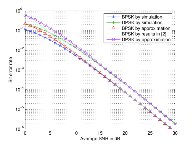
Figure 1: BERs of BPSK and DPSK under Nakagami-$m$ fading with $m=2$

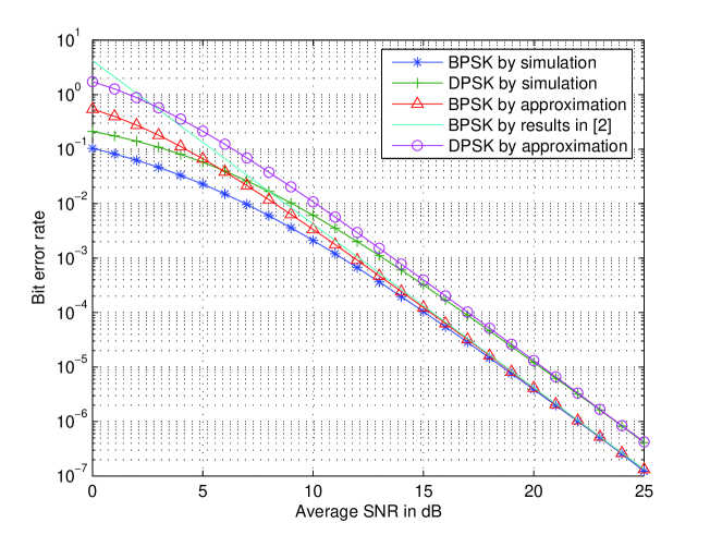
Figure 2: BERs of BPSK and DPSK under Nakagami-$m$ fading with $m=3$

In summary, for the two cases analyzed above, the asymptotic error rate expressions in (3) and (6) are given by $C_{1}F(C_{2}\rho^{-1})\sim C_{1}C_{2}^{d}F(\rho^{-1})$ with constants $C_{1}$ and $C_{2}$. Knowing that outage event occurs when the instantaneous SNR $\rho z$ falls below certain threshold, and since $F(C_{2}\rho^{-1})$ is the probability that $\rho z$ falls below $C_{2}$, the asymptotic error rate expression $C_{1}F(C_{2}\rho^{-1})$ represents a scaled version of the outage probability. Furthermore, $C_{1}$ and $C_{2}$ depend only on the system specifications ($\alpha$, $\beta$, $\theta_{\rm t}$, $g_{1}(\theta)$ and $g_{2}(\theta)$) and the variation exponent $d$ of $F(z)$. As a result, we only need to know $d$ in addition to $F(z)$ to obtain the asymptotic error rate and do not need to express $F(z)$ or the corresponding PDF $f(z)$ in series expansion form. For simple practical channels like Nakagami-$m$, $d=m$ can be seen by inspection of $F(z)$ or $f(z)$. For many channel distributions, the diversity order can also be obtained by solving $\lim_{z\rightarrow 0}F(\tau z)/F(z)=\tau^{d}$ or $\lim_{z\rightarrow 0}f(\tau z)/f(z)=\tau^{d-1}$ using L’Hôpital’s rule, or approximated numerically by evaluating $\lim_{z\rightarrow 0}\log F(z)/\log z=d$ or $\lim_{z\rightarrow 0}\log f(z)/\log z=d-1$. Therefore, the asymptotic error rate is related to the channel distribution in many useful ways which complement the PDF-based approach in [2]. In Figures 1 and 2, we compare the BERs of DPSK and BPSK under Nakagami-$m$ fading obtained through Monte Carlo simulation, with their approximations given by (3) and (6). We observe that the results given by (3) and (6) match their corresponding simulation results within $0.1$ dB at error rates of $10^{-6}$. In addition, it can be seen that our approach gives better approximation to the Monte Carlo simulation results than [2], most noticeably for moderate values of average SNR.

There are some practical cases of instantaneous error rate ${\rm P_{e}}(\rho z)$, which do not fit AS1c but can be expressed as linear combinations of exponential-mixture functions of $\rho z$ in the form $\int_{0}^{\theta_{\rm t}}g_{2}(\theta)\exp(-\rho z/g_{1}(\theta))d\theta$ given in AS1c, such as the instantaneous BER of Gray-coded $M$-PSK [15, Section 8.1.1.3]. There are also practical ${\rm P_{e}}(\rho z)$ which fits AS1c, but can be expressed as a linear combination of exponential-mixture functions, each with a much simpler $g_{2}(\theta)$ function than that of ${\rm P_{e}}(\rho z)$ itself, such as the instantaneous SER of square $M$-QAM. For these cases, asymptotic characterization of ${\rm\overline{P}_{e}}(\rho)$ through linear combination becomes necessary. Specifically, for an instantaneous error rate given by ${\rm P_{e}}(\rho z)=\sum_{j=1}^{J}a_{j}{\rm P_{e}}_{,j}(\rho z)$ where $\{a_{j}\}_{j=1}^{J}$ are constants and $\{{\rm P_{e}}_{,j}(\rho z)\}_{j=1}^{J}$ are (simpler) expressions satisfying AS1b or AS1c, we first determine ${\rm E}[{\rm P_{e}}_{,j}(\rho z)]\sim C_{1j}F(C_{2j}\rho^{-1})$ using the methods in this section. If $\{a_{j}\}_{j=1}^{J}$ are all positive, we have ${\rm\overline{P}_{e}}(\rho)\sim\sum_{j=1}^{J}a_{j}C_{1j}F(C_{2j}\rho^{-1})$; if any of $\{a_{j}\}_{j=1}^{J}$ is negative, ${\rm\overline{P}_{e}}(\rho)\sim\sum_{j=1}^{J}a_{j}C_{1j}C_{2j}^{d}F(\rho^{-1})$ can be established. We omit the derivations due to lack of space.

VI Asymptotic Error Rate Performance under Diversity Combining

In this section, we establish an extension and application of the results derived in Section V-B, by analyzing the asymptotic error rate performance at high average SNR for several diversity combining schemes. The results are especially useful when the diversity branches have non-identical fading distributions and when the average error rate expression is not available in closed form.

We consider a system in which the receiver has the channel state information (CSI), and employs $N$ diversity branches with independent but not necessarily identical fading distributions. Particularly, the $n$-th branch is assumed to have a channel power gain $z_{n}$ with CDF $F_{n}(z)=z^{d_{n}}l_{n}(z)$ where $l_{n}(z)$ is slowly varying at $0$. We derive asymptotic expressions for E$[\beta e^{-\alpha\rho z_{\rm c}}]$ and E$[\int_{0}^{\theta_{\rm t}}g_{2}(\theta)\exp(-\rho z/g_{1}(\theta))d\theta]$ for large $\rho$ in terms of the system specifications ($\alpha$, $\beta$, $\theta_{\rm t}$, $g_{1}(\theta)$ and $g_{2}(\theta)$), $\rho$, $\{d_{n}\}_{n=1}^{N}$ and $\{l_{n}(\cdot)\}_{n=1}^{N}$, where $z_{\rm c}$ is the channel power gain after combining. In order to address this problem with a unified approach, we first determine the asymptotic CDF of $z_{\rm c}$ near the origin in the form $F_{\rm c}(z)\sim z^{d_{\rm c}}l_{\rm c}(z)$ with $l_{\rm c}(z)$ being slowly varying at $0$ for each specific diversity combining scheme by expressing $d_{\rm c}$ and $l_{\rm c}(\cdot)$ in terms of $\{d_{n}\}_{n=1}^{N}$ and $\{l_{n}(\cdot)\}_{n=1}^{N}$ respectively. Moreover, we express the CDF of the combined channel $F_{\rm c}(z)$ in terms of $\{d_{n}\}_{n=1}^{N}$ and $\{F_{n}(\cdot)\}_{n=1}^{N}$. This will lead to characterizing E$[\beta e^{-\alpha\rho z_{\rm c}}]$ and E$[\int_{0}^{\theta_{\rm t}}g_{2}(\theta)\exp(-\rho z/g_{1}(\theta))d\theta]$ in terms of the system specifications, $\rho$, $d_{\rm c}$ and $l_{\rm c}(\cdot)$ (and alternatively $F_{\rm c}(\cdot)$) using the same method as in Section V-B.

VI-A Maximum Ratio Combining (MRC)

For MRC with independent branches as well as a number of cooperative relay systems [19], the channel power gain can be expressed as the sum of independent random variables: $z_{\rm c}=\sum_{n=1}^{N}z_{n}$. Define $\mathcal{L}_{n}(s):=\int_{0}^{\infty}e^{-sz}dF_{n}(z)$ and $\mathcal{L}_{\rm c}(s):=\int_{0}^{\infty}e^{-sz}dF_{\rm c}(z)$ to be the Laplace-Stieltjes transforms of the respective distributions. Based on the convolution property of Laplace transform, we have $\mathcal{L}_{\rm c}(s)=\prod_{n=1}^{N}\mathcal{L}_{n}(s)$. On the other hand, it follows from Tauberian theorem (Theorem 2) that $\mathcal{L}_{n}(s)\sim\Gamma(d_{n}+1)s^{-d_{n}}l_{n}(s^{-1})$ as $s\rightarrow\infty$, and therefore $\mathcal{L}_{\rm c}(s)\sim\prod_{n=1}^{N}\Gamma(d_{n}+1)\cdot s^{-\sum_{n=1}^{N}d_{n}}\prod_{n=1}^{N}l_{n}(s^{-1})$. It is easy to verify that $\prod_{n=1}^{N}\Gamma(d_{n}+1)\cdot\prod_{n=1}^{N}l_{n}(s^{-1})$ is slowly varying at $\infty$ as a function of $s$. It follows from Tauberian theorem (Theorem 2) that

$$F_{\rm c}(z)\sim\left[\Gamma\left(\sum_{n=1}^{N}d_{n}+1\right)\right]^{-1}\prod_{n=1}^{N}\Gamma(d_{n}+1)\cdot\prod_{n=1}^{N}F_{n}(z)$$ (7)

near the origin, where we have simplified $z^{\sum_{n=1}^{N}d_{n}}\prod_{n=1}^{N}l_{n}(z)$ as $\prod_{n=1}^{N}F_{n}(z)$, and the first factor on the right hand side is due to the variation exponent $-\sum_{n=1}^{N}d_{n}$ of $\mathcal{L}_{\rm c}(s)$ at $\infty$. We will relate the outage of the combined channel in (7) to the average error rates in Section VI-D.

VI-B Equal Gain Combining (EGC)

For EGC with independent branches we have $z_{\rm c}=(\sum_{n=1}^{N}\sqrt{z_{n}})^{2}/N$. Define $y_{n}=\sqrt{z_{n}}$ and $y_{\rm c}=\sum_{n=1}^{N}y_{n}$. It is easy to derive that $y_{n}$ has a CDF given by $G_{n}(y)=y^{2d_{n}}l(y^{2})$, and show that $l(y^{2})$ is slowly varying as a function of $y$ at $0$. Consequently, by using the same method as in Section VI-A, we can derive the asymptotic CDF $G_{\rm c}(y)\sim[\Gamma(2\sum_{n=1}^{N}d_{n}+1)]^{-1}\prod_{n=1}^{N}\Gamma(2d_{n}+1)\cdot y^{2\sum_{n=1}^{N}d_{n}}\prod_{n=1}^{N}l_{n}(y^{2})$ of $y_{\rm c}$ near $y_{\rm c}=0$, then using $z_{\rm c}=y_{\rm c}^{2}/N$, we get the asymptotic CDF

$$F_{\rm c}(z)\sim\left[\Gamma\left(2\sum_{n=1}^{N}d_{n}+1\right)\right]^{-1}\prod_{n=1}^{N}\Gamma(2d_{n}+1)\cdot\prod_{n=1}^{N}F_{n}(Nz)$$ (8)

of $z_{\rm c}$ near the origin, which will be related to the asymptotic error rates in Section VI-D.

VI-C Selection Combining (SC)

For SC with independent branches we have $z_{\rm c}=\max_{n=1,2,...,N}\{z_{n}\}$, then it follows that

$$F_{\rm c}(z)=\prod_{n=1}^{N}F_{n}(z)=z^{\sum_{n=1}^{N}d_{n}}\prod_{n=1}^{N}l_{n}(z),$$ (9)

which will be used to derive the asymptotic error rates next.

VI-D Asymptotic Error Rate Expressions

For all three cases analyzed above, we can verify that $F_{\rm c}(z)$ is regularly varying at $0$ with exponent $d_{\rm c}=\sum_{n=1}^{N}d_{n}>0$, since the same holds for $F_{n}(z)$ with exponent $d_{n}>0$. In Section V-B we established the asymptotic average error rates in terms of the CDF $F(z)$ in closed-form. We can directly apply these results here to the combined CDFs of the respective diversity combining schemes, and obtain

$${\rm E}[\beta e^{-\alpha\rho z_{\rm c}}]\sim\beta\Gamma(d_{\rm c}+1)F_{\rm c}(\alpha^{-1}\rho^{-1})$$ (10)

$${\rm E}\left[\int_{0}^{\theta_{\rm t}}g_{2}(\theta)\exp\left(-\frac{\rho z}{g_{1}(\theta)}\right)d\theta\right]\sim\left(\Gamma(d_{\rm c}+1)\int_{0}^{\theta_{\rm t}}g_{2}(\theta)g_{1}^{d_{\rm c}}(\theta)d\theta\right)F_{\rm c}(\rho^{-1})$$ (11)

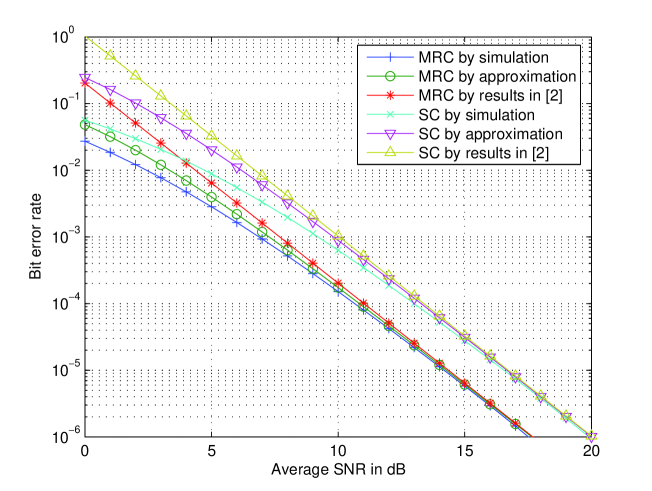
Figure 3: BERs of BPSK under MRC and SC involving three Nakagami-$m$ fading branches with $m=0.5$, $1$ and $1.5$

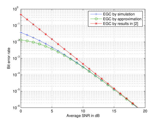
Figure 4: BERs of BPSK under EGC involving three Nakagami-$m$ fading branches with $m=0.5$, $1$ and $1.5$

as $\rho\rightarrow\infty$, where $d_{\rm c}$ is the same for all three combining schemes, and $F_{\rm c}(\cdot)$ is given by (7), (8) or (9) for MRC, EGC and SC respectively. We have thus established a unified approach to evaluate the asymptotic error rate at high average SNR for MRC, EGC and SC, given the conditions that the channel power gain of each branch has a CDF which is regularly varying at $0$ and the instantaneous error rate can be expressed as linear combination of exponential or exponential-mixture functions. Figures 3 and 4 show the BERs of BPSK under different diversity combining schemes obtained through Monte Carlo simulation, as well as their approximations obtained through (11) together with (7), (8) and (9). The accuracy of our approach is corroborated by the closeness (within $0.2$ dB at error rate of $10^{-6}$) between the simulation results and analytical asymptotic approximations. Like observed in Figures 1 and 2, our approach gives better approximation than [2] to the simulation results, especially when the average SNR is not significantly high.

In addition to the simple relation between the asymptotic error rate and the channel distribution, it can be seen that our approach based on Tauberian theorem enables analysis of the performance of a communication system involving multiple channels, in which the regular variation property of the distribution of the overall effective channel is inherited from the channel distributions corresponding to the constituent parts of the system. Also, the asymptotic CDFs given by (7) and (8) can make high-SNR substitutes of the numerical inversion method in [20] to compute outages in fading channels, as long as different diversity branches are independent.

VII Conclusions

In this paper, we investigate the relationship between the high-SNR asymptotic average error rate and outage by establishing that the instantaneous error rate being upper bounded by an exponential function of the instantaneous SNR is sufficient for outage events to dominate error rate performance. We do this by establishing the regular/rapid variation of the CDF of the channel power gain with exponent $d$ at $0$ to be a necessary and sufficient condition for the error rate to exhibit a diversity order of $d$. This implies the equivalence between the error-rate-based diversity order and the outage-based diversity order, thereby characterizing the conditions under which the outage event dominates high-SNR error rate performance. For the case of finite $d$, the constant SNR offset between different communication systems over the same fading channel with exponentially bounded instantaneous error rates is revealed. For instantaneous error rates given by a mixture of exponential functions of the instantaneous SNR (AS1c), we express the high-SNR asymptotic error rates directly as multiples of the outage probability (channel CDF for small arguments). Furthermore, we derive the asymptotic error rate for instantaneous error rate satisfying AS1c, considering different diversity combining schemes with the CDF of the channel power gain of each diversity branch being regularly varying at $0$. All these results exhibit the convenience and effectiveness of Tauberian theorem as a tool to analyze the asymptotic error rate performance related to diversity under fading, thus conveniently generalizing and complementing the PDF-based approach in [2]. Numerical results show that our approach gives more accurate approximations than [2].

Appendix A Proof of Proposition 2

We prove this for $H(x)$ being slowly varying at $\infty$ only, since the case of slow variation at $0$ can be obtained by considering $H(x^{-1})$. By definition we have $\lim_{x\rightarrow\infty}H(tx)/H(x)=1$ for $t>0$, which implies that for any $\epsilon_{1}>0$, there exists sufficiently large $s_{1}$ such that for all $x>s_{1}$, $|H(tx)/H(x)-1|<\epsilon_{1}$. Without loss of generality we assume $t>1$, and since $0\leq h_{1}\leq H(x)\leq h_{2}<\infty$ for sufficiently large $x$ (say $x>s_{2}$), it follows that for any $\epsilon_{2}=\epsilon_{1}h_{2}$, there exists sufficiently large $s_{3}=\max\{s_{1},s_{2}\}$ such that for all $x_{1}>s_{3}$ and $x_{2}>s_{3}$, $|H(x_{2})-H(x_{1})|<\epsilon_{2}$. This follows from multiplying $|H(tx)/H(x)-1|<\epsilon_{1}$ by $H(x)$. Therefore the Cauchy criteria for the existence of limit is satisfied, and $H(x)$ should converge to a constant in $[h_{1},h_{2}]$ as $x\rightarrow\infty$.

Appendix B Proof of Proposition 3

We use Theorem 1 to prove the relation between (2b) and (2c), starting from the claim that (2b) implies (2c). For $0<d\leq\infty$, (2b) implies that ${\rm\overline{P}_{e}}(\rho)$ has a variation exponent $-d$ at $\infty$, and thus can be represented as

$${\rm\overline{P}_{e}}(\rho)=c(\rho)\exp\left\{\int_{a}^{\rho}\frac{\epsilon(u)}{u}du\right\}$$ (12)

for some $a>0$, $c(\rho)\rightarrow c\in(0,\infty)$ and $\epsilon(\rho)\rightarrow-d$ as $\rho\rightarrow\infty$, using Theorem 1. Therefore

$$\begin{split}\lim_{\rho\rightarrow\infty}\frac{\log{\rm\overline{P}_{e}}(\rho)}{\log\rho}&=\lim_{\rho\rightarrow\infty}\frac{\log c(\rho)+\int_{a}^{\rho}\frac{\epsilon(u)}{u}du}{\log\rho}=\lim_{\rho\rightarrow\infty}\frac{\int_{a}^{\rho}\frac{\epsilon(u)}{u}du}{\log\rho}\\ &=\lim_{\rho\rightarrow\infty}\frac{\epsilon(\rho)}{\rho}(\rho^{-1})^{-1}=\lim_{\rho\rightarrow\infty}\epsilon(\rho)=-d\end{split}$$ (13)

where in the second equality we used $\epsilon(\rho)\rightarrow-d$, and in the third equality L’Hôpital’s rule. We have thus shown that (2b) implies (2c).

We next prove that (2c) implies (2b) given the mild additional assumption that the limit in (2b) exists. The existence of the limit in (2b) implies that $\lim_{\rho\rightarrow\infty}{\rm\overline{P}_{e}}(\tau\rho)/{\rm\overline{P}_{e}}(\rho)=\tau^{m_{1}}$ for some $m_{1}\in[-\infty,\infty]$ [8, Lemma 1, p.275]. We would like to show that $m_{1}=-d$. Clearly, ${\rm\overline{P}_{e}}(\rho)$ can be represented by (12) for some $a>0$, $c(\rho)\rightarrow c\in(0,\infty)$ and $\epsilon(\rho)\rightarrow m_{1}$ as $\rho\rightarrow\infty$. Similar to (13), it can be derived that $\lim_{\rho\rightarrow\infty}(\log{\rm\overline{P}_{e}}(\rho))/(\log\rho)=m_{1}$. Given the condition that (2c) holds, it follows that $m_{1}=-d$, and thus (2b) also holds.

To show that (2a) is a special case of (2b), from (2a) we get ${\rm\overline{P}_{e}}(\tau\rho)=G^{-d}\tau^{-d}\rho^{-d}+o(\rho^{-d})$, then

$$\lim_{\rho\rightarrow\infty}\frac{{\rm\overline{P}_{e}}(\tau\rho)}{{\rm\overline{P}_{e}}(\rho)}=\lim_{\rho\rightarrow\infty}\frac{G^{-d}\tau^{-d}+o(\rho^{-d})/\rho^{-d}}{G^{-d}+o(\rho^{-d})/\rho^{-d}}=\tau^{-d}$$ (14)

i.e. (2b) holds. An example for why (2b) does not imply (2a) can be seen for the case ${\rm\overline{P}_{e}}(\rho)\sim c_{1}(\log\rho)^{c_{2}}\rho^{-d}$ with $c_{1},c_{2}>0$, as brought up in [6, 7]. Hence (2b) is more general than (2a).

Appendix C Proof of Theorem 3

We begin with assuming the regular/rapid variation of $F(z)$ with exponent $d$ at $0$, and proving the regular/rapid variation of ${\rm\overline{P}_{e}}(\rho)$ with exponent $-d$ at $\infty$, by analyzing the upper and lower bounds of ${\rm\overline{P}_{e}}(\rho)$. Due to AS1a we have

$${\rm\overline{P}_{e}}(\rho)=\int_{0}^{\infty}{\rm P_{e}}(\rho z)dF(z)\leq\int_{0}^{\infty}\beta e^{-\alpha\rho z}dF(z)={\rm\overline{P}_{e,UB}}(\rho)$$ (15)

and since ${\rm P_{e}}(\cdot)$ is non-negative and monotonically decreasing,

$${\rm\overline{P}_{e}}(\rho)\geq\int_{0}^{\eta/\rho}{\rm P_{e}}(\rho z)dF(z)\geq\int_{0}^{\eta/\rho}{\rm P_{e}}(\eta)dF(z)={\rm P_{e}}(\eta)F(\eta/\rho)={\rm\overline{P}_{e,LB}}(\rho)$$ (16)

for any constant $\eta>0$. It follows from (15) and (16) that

$$\frac{\log{\rm\overline{P}_{e,LB}}(\rho)}{\log\rho}\leq\frac{\log{\rm\overline{P}_{e}}(\rho)}{\log\rho}\leq\frac{\log{\rm\overline{P}_{e,UB}}(\rho)}{\log\rho}$$ (17)

For $d=\infty$, it can be easily seen that ${\rm\overline{P}_{e,LB}}(\rho)$ has variation exponent $-\infty$ at $\rho=\infty$ and thus satisfies (2c). Also, based on Tauberian theorem (Theorem 2) with the correspondences $F(z)\equiv H(x)$ and $\alpha\rho\equiv s$, ${\rm\overline{P}_{e,UB}}(\rho)$ has variation exponent $-\infty$ at $\rho=\infty$ and thus satisfies (2c). By taking the limit of (17) as $\rho\rightarrow\infty$ and using Squeeze theorem (a well-known theorem stating that if $\lim_{x\rightarrow a}H_{1}(x)=\lim_{x\rightarrow a}H_{3}(x)=h$ and $H_{1}(x)\leq H_{2}(x)\leq H_{3}(x)$ in some neighborhood of $a$, then $\lim_{x\rightarrow a}H_{2}(x)=h$), it follows that ${\rm\overline{P}_{e}}(\rho)$ should satisfy (2c).

For $0<d<\infty$, let $F(z)=z^{d}l(z)$ with $l(z)$ being slowly varying at $0$. Based on (15) and Tauberian theorem (Theorem 2) we have

$${\rm\overline{P}_{e,UB}}(\rho)\sim\beta\Gamma(d+1)(\alpha\rho)^{-d}l(\alpha^{-1}\rho^{-1}).$$ (18)

Also, it follows from (16) that

$${\rm\overline{P}_{e,LB}}(\rho)=\eta^{d}\rho^{-d}{\rm P_{e}}(\eta)l(\eta/\rho).$$ (19)

It is easy to verify that both ${\rm\overline{P}_{e,UB}}(\rho)$ and ${\rm\overline{P}_{e,LB}}(\rho)$ satisfy (2b), thus also satisfy (2c) due to Proposition 3, then ${\rm\overline{P}_{e}}(\rho)$ should satisfy (2c) due to (17). This completes the sufficiency part.

We now show ${\rm\overline{P}_{e}}(\rho)$ being regularly/rapidly varying with exponent $-d$ at $\infty$ implies $F(z)$ being regularly/rapidly varying with exponent $d$ at $0$ provided that $F(z)$ is a Karamata function (at $0$). Based on [8, Lemma 1, p.275], it can be confirmed that $\lim_{z\rightarrow 0}F(\tau z)/F(z)=\tau^{m_{2}}$ with $m_{2}\in(0,\infty]$ being the variation exponent of $F(z)$. Like in the sufficiency part of the proof, it can be derived that both ${\rm\overline{P}_{e,UB}}(\rho)$ and ${\rm\overline{P}_{e,LB}}(\rho)$ have variation exponent $-m_{2}$, then (17) becomes $-m_{2}\leq-d\leq-m_{2}$, leading to $m_{2}=d$. Therefore $F(z)$ is regularly/rapidly varying with exponent $d$ at $0$.

Appendix D Proof of Theorem 4

We first derive the asymptotic expression for ${\rm\overline{P}_{e}}(\rho)$ assuming AS2b, $F(z)=z^{d}l(z)$. Theorem 3 implies that ${\rm\overline{P}_{e}}(\rho)=\rho^{-d}r(\rho)$ where $r(\rho)$ is slowly varying at $\infty$. Let $l_{1}(\rho):={\rm\overline{P}_{e}}(\rho)/(\rho^{-d}l(\rho^{-1}))$. It is easy to show that $l_{1}(\rho)$ is slowly varying at $\infty$. On the other hand, from (15) and (16) we have ${\rm\overline{P}_{e,LB}}(\rho)/(\rho^{-d}l(\rho^{-1}))\leq l_{1}(\rho)\leq{\rm\overline{P}_{e,UB}}(\rho)/(\rho^{-d}l(\rho^{-1}))$; also, based on (18) and (19) as well as the definition of slow variation, we have $\lim_{\rho\rightarrow\infty}{\rm\overline{P}_{e,UB}}(\rho)/(\rho^{-d}l(\rho^{-1}))=\beta\alpha^{-d}\Gamma(d+1)$ and $\lim_{\rho\rightarrow\infty}{\rm\overline{P}_{e,LB}}(\rho)/(\rho^{-d}l(\rho^{-1}))={\rm P_{e}}(\eta)\eta^{d}$ respectively. It follows that for sufficiently large $\rho$, $l_{1}(\rho)$ is bounded between two finite positive constants. Based on Proposition 2, $l_{1}(\rho)$ converges to a finite positive constant as $\rho\rightarrow\infty$, say $l_{1}(\rho)\sim c_{1}\in(0,\infty)$, and hence ${\rm\overline{P}_{e}}(\rho)\sim c_{1}\rho^{-d}l(\rho^{-1})$.

Consider now the derivation for the asymptotic expression of $F(z)$ assuming ${\rm\overline{P}_{e}}(\rho)=\rho^{-d}r(\rho)$ and that $\lim_{z\rightarrow 0}F(\tau z)/F(z)$ exists for $\tau>0$. It follows directly from Theorem 3 that $F(z)$ must be in the form $F(z)=z^{d}l(z)$ with $l(z)$ slowly varying at $0$. Based on the sufficiency part of the proof (i.e. the asymptotic expression of ${\rm\overline{P}_{e}}(\rho)$ given $F(z)=z^{d}l(z)$), we must have ${\rm\overline{P}_{e}}(\rho)/(\rho^{-d}l(\rho^{-1}))=r(\rho)/l(\rho^{-1})\sim c_{1}$ as $\rho\rightarrow\infty$, with constant $c_{1}\in(0,\infty)$. Consequently, $l(z)/r(z^{-1})\sim c_{1}^{-1}$ as $z\rightarrow 0$, and $F(z)\sim c_{2}z^{d}r(z^{-1})$ where $c_{2}=c_{1}^{-1}\in(0,\infty)$ is a constant.

References

- [1] A. J. Goldsmith, Wireless Communications, 1st ed. Cambridge: Cambridge University Press, Aug. 2005.
- [2] Z. Wang and G. B. Giannakis, “A simple and general parameterization quantifying performance in fading channels,” IEEE Transactions on Communications, vol. 51, no. 8, pp. 1389–1398, Aug. 2003.
- [3] L. G. Ordonez, D. P. Palomar, A. Pages-Zamora, and J. R. Fonollosa, “High-SNR Analytical Performance of Spatial Multiplexing MIMO Systems With CSI,” IEEE Transactions on Signal Processing, vol. 55, no. 11, pp. 5447–5463, Nov. 2007.
- [4] L. Zhao, W. Mo, Y. Ma, and Z. Wang, “Diversity and Multiplexing Tradeoff in General Fading Channels,” IEEE Transactions on Information Theory, vol. 53, no. 4, pp. 1549–1557, Apr. 2007.
- [5] L. Zheng and D. N. C. Tse, “Diversity and multiplexing: A fundamental tradeoff in multiple-antenna channels,” IEEE Transactions on Information Theory, vol. 49, no. 5, pp. 1073–1096, May. 2003.
- [6] M. Taherzadeh, A. Mobasher, and A. K. Khandani, “LLL Reduction Achieves the Receive Diversity in MIMO Decoding,” IEEE Transactions on Information Theory, vol. 53, no. 12, pp. 4801–4805, Dec. 2007.
- [7] M. Taherzadeh and A. K. Khandani, “On the Limitations of the Naive Lattice Decoding,” IEEE Transactions on Information Theory, vol. 56, no. 10, pp. 4820–4826, Oct. 2010.
- [8] W. Feller, An Introduction to Probability Theory and Its Applications: Volume II, 2nd ed. New York: John Wiley and Sons, 1971.
- [9] N. H. Bingham, C. M. Goldie, and J. L. Teugels, Regular Variation. Cambridge University Press, Jul. 1989.
- [10] B. Zwart, S. Borst, and M. Mandjes, “Exact queueing asymptotics for multiple heavy-tailed on-off flows,” IEEE INFOCOM, vol. 1, pp. 279–288, Apr. 2001.
- [11] P. Jelenkovic and P. Momcilovic, “Capacity regions for network multiplexers with heavy-tailed fluid on-off sources,” IEEE INFOCOM, vol. 1, pp. 289–298, Apr. 2001.
- [12] D. Gesbert and M. Kountouris, “Rate Scaling Laws in Multicell Networks under Distributed Power Control and User Scheduling,” IEEE Transactions on Information Theory, vol. 57, no. 1, pp. 234–244, Jan. 2011.
- [13] Y. Zhang and C. Tepedelenlioglu, “Applications of Tauberian Theorem for High-SNR Analysis of Performance over Fading Channels,” Presented at IEEE 12th International Workshop on Signal Processing Advances in Wireless Communications.
- [14] A. Dembinska and A. Stepanov, “Limit theorems for the ratio of weak records,” Statistics and Probability Letters, vol. 76, no. 14, pp. 1454–1464, Aug. 2006.
- [15] M. K. Simon and M.-S. Alouini, Digital Communication over Fading Channels: A Unified Approach to Performance Analysis, 1st ed. John Wiley and Sons, 2000.
- [16] P. S. Bithas, N. C. Sagias, P. T. Mathiopoulos, G. K. Karagiannidis, and A. A. Rontogiannis, “On the performance analysis of digital communications over generalized-K fading channels,” IEEE Communications Letters, vol. 10, no. 5, pp. 353–355, May. 2006.
- [17] H. A. Suraweera and G. K. Karagiannidis, “Closed-form error analysis of the non-identical Nakagami-m relay fading channel,” IEEE Communications Letters, vol. 12, no. 4, pp. 259–261, Apr. 2008.
- [18] M. A. Chaudhry and S. M. Zubair, On a Class of Incomplete Gamma Functions with Applications, 1st ed. Chapman and Hall/CRC, Aug. 2001.
- [19] P. A. Anghel and M. Kaveh, “Exact symbol error probability of a Cooperative network in a Rayleigh-fading environment,” IEEE Transactions on Wireless Communications, vol. 3, no. 5, pp. 1416–1421, Sep. 2004.
- [20] Y.-C. Ko, M.-S. Alouini, and M. K. Simon, “Outage probability of diversity systems over generalized fading channels,” IEEE Transactions on Communications, vol. 48, no. 11, pp. 1783–1787, Nov. 2000.