Fluctuation phenomena, random processes, noise, and Brownian motion Nonequilibrium and irreversible thermodynamics

Work fluctuations for a harmonic oscillator driven by an external random force

Abstract

The fluctuations of the work done by an external Gaussian random force on a harmonic oscillator that is also in contact with a thermal bath is studied. We have obtained the exact large deviation function as well as the complete asymptotic forms of the probability density function. The distribution of the work done are found to be non-Gaussian. The steady state fluctuation theorem holds only if the ratio of the variances, of the external random forcing and the thermal noise respectively, is less than 1/3. On the other hand, the transient fluctuation theorem holds (asymptotically) for all the values of that ratio. The theoretical asymptotic forms of the probability density function are in very good agreement with the numerics as well as with an experiment.

One of the most fundamental and important problems in the nonequilibrium physics is to understand fluctuations. In this context, the so-called fluctuation theorem (FT) has generated a lot of interest. The FT was found first for the phase space contraction in dynamical systems [1, 2] and later for a certain “action functional” in stochastic systems [3, 4] — these quantities are generally referred to as the “entropy production”. Subsequently, there has been an increased interest in the FTs for various physical quantities such as work, power flux, heat flow, total entropy, etc. [5, 6, 7] — because, in the absence of a general framework for nonequilibrium phenomena, the FTs seem to be providing an unifying picture for a variety of nonequilibrium systems. The so-called Jarzynski equality [8], Crooks relation [9], and Hatano-Sasa identity [10] are closely related to the FT. In the linear response regime, the FT leads to the Green-Kubo formula and the Onsager reciprocity relations [4, 11]. However, the FT is more general, as it also describes fluctuations in the nonlinear regime arbitrarily far from the equilibrium.

The FT relates the positive and the negative fluctuations of a certain time-integrated physical quantity $W_{\tau}=\int_{0}^{\tau}\dot{W}(t)\,dt$, during a nonequilibrium process, according to:

$$\lim_{\tau\rightarrow\infty}\frac{1}{\tau}\ln\biggl{[}\frac{P(W_{\tau}=w\tau)}{P(W_{\tau}=-w\tau)}\biggr{]}=w,$$ (1)

where $P(W_{\tau}=\pm w\tau)$ is the probability density function (PDF) of the physical quantity $W_{\tau}$ to have a value $\pm w\tau$. In fact, depending on the choice of the initial ensemble, there are two kinds of FTs: the transient fluctuation theorem (TFT) — in which the system at $\tau=0$ is in equilibrium, and the steady state fluctuation theorem (SSFT) — in which the quantity $W_{\tau}$ is computed in a time interval $\tau$ in the nonequilibrium steady state. Usually, the TFT is stated for a finite $\tau$, i.e., without the limit $\tau\rightarrow\infty$ in eq. (1). Naively, one would expect the TFT and the SSFT to become equivalent in the $\tau\rightarrow\infty$ limit. However, this is not always correct.

There have been several experimental tests of the FT and related results, in diverse systems such as a colloidal particle in a changing optical trap [12, 13, 14], liquid crystal electroconvection [15], fluidized granular medium [16], electrical circuits [17], RNA stretching [18, 19], sheared micellar gel [20], harmonic oscillator [21], self-propelled polar particle [22], wave Turbulence [23], and a gravitational wave detector [24]. A recent review of the experimental applications of the FTs may be found in ref. [25]. Interpretation of experimental findings are not always easy as the FTs are governed by the atypical fluctuations that correspond to the tails of the probability distributions — and in an experiment in a finite time, it is often hard to acquire enough of the rare events to produce the tail of the distribution accurately. Therefore, it is very important to have exact theoretical predictions.

Theoretical investigations of the work FTs so far have been mostly limited to the systems describe by linear Langevin equations with a Gaussian white thermal noise and driven out of equilibrium by an external deterministic force. In such cases [6], the distributions of the work done by the external force are Gaussian and hence the work FTs hold somewhat trivially. On the contrary, the distributions of the work done by an external Gaussian stochastic force have been found to be non-Gaussian in recent experiments on systems coupled to a thermal bath and driven out of equilibrium by an external random force [26]. Motivated by these experiments, in this Letter, we address the important question regarding the role of the external stochastic forcing on the work fluctuations.

We consider one of the most basic physical systems, namely, the harmonic oscillator. We investigate the fluctuations of the work done by an externally applied Gaussian random force on a harmonic oscillator that is also in contact with a thermal bath. The displacement $x(t)$ of the harmonic oscillator from its mean position is described by the Langevin equation

$$m\frac{d^{2}x}{dt^{2}}+\gamma\frac{dx}{dt}+kx=\zeta_{T}(t)+f_{0}(t),$$ (2)

where $m$ is the mass, $\gamma$ is the viscous drag coefficient and $k$ is the spring constant. The interaction with the thermal bath is modeled by a Gaussian white noise $\zeta_{T}(t)$ with zero-mean $\langle\zeta_{T}(t)\rangle=0$. The externally applied force $f_{0}(t)$ is again a Gaussian random variable with $\langle f_{0}(t)\rangle=0$, and $\zeta_{T}$ and $f_{0}$ are uncorrelated. Equation (2) is asymmetric in $\zeta_{T}$ and $f_{0}$ — the fluctuation-dissipation theorem relates the thermal fluctuation to the viscous drag as $\langle\zeta_{T}(s)\zeta_{T}(t)\rangle=2D\delta(s-t)$ where $D=\gamma k_{B}T$ with $T$ being the temperature of the bath and $k_{B}$ being the Boltzmann constant, whereas the fluctuation of the external force $\langle f_{0}(s)f_{0}(t)\rangle=(\delta f_{0})^{2}\delta(s-t)$ is independent of $\gamma$. As it turns out, the only relevant parameter is

$$\alpha=\frac{(\delta f_{0})^{2}}{2D}=\frac{\langle x^{2}\rangle}{\langle x^{2}\rangle_{\text{eq}}}-1,\quad\text{and}~{}\alpha\in(0,\infty),$$ (3)

where $\langle x^{2}\rangle$ and $\langle x^{2}\rangle_{\text{eq}}$ are the variance of $x$ in the steady-state (for $f_{0}\not=0$) and in equilibrium (for $f_{0}=0$) respectively.

The quantity of interest is the work done by the external random force $f_{0}(t)$ on the harmonic oscillator in a time interval $\tau$, in the nonequilibrium steady state. This is given (in units of $k_{B}T$) by

$$W_{\tau}=\frac{1}{k_{B}T}\int_{0}^{\tau}f_{0}(t)\frac{dx}{dt}\,dt,$$ (4)

with the initial condition (at $\tau=0$) drawn from the steady state distribution. Evidently, $W_{\tau}$ is a fluctuating quantity whose value depends on the initial condition, the trajectories of thermal noise $\{\zeta_{T}(t):0\leq t\leq\tau\}$ and the external random force $\{f_{0}(t):0\leq t\leq\tau\}$, during any particular realization.

It is clear from eq. (2) that both the displacement $x$ and the velocity $v=dx/dt$ depend linearly on the thermal noise and the external random force. Therefore, the distribution of the phase space variables $(x,v)$ is a Gaussian whose covariance matrix can be easily evaluated from eq. (2). However, due to the nonlinear dependence of the work given by eq. (4), on the thermal noise and the external random forcing, the PDF $P(W_{\tau})$ is not expected to be Gaussian — although for any fixed realizations of $\{f_{0}(t)\}$ the work fluctuation would be Gaussian. Nonetheless, one expects the large deviation form [27]

$$P(W_{\tau}=w\tau/\tau_{\gamma})\sim e^{(\tau/\tau_{\gamma})\,h(w)}\quad\text{for}~{}\tau\gg\tau_{\gamma},$$ (5)

where $\tau_{\gamma}=m/\gamma$ is the viscous relaxation time and $h(w)$ is the large deviation function (LDF), which is defined by

$$h(w)=\lim_{(\tau/\tau_{\gamma})\rightarrow\infty}\frac{1}{(\tau/\tau_{\gamma})}\ln P(W_{\tau}=w\tau/\tau_{\gamma}).$$ (6)

The FT as given by  eq. (1) is equivalent to the symmetry relation

$$h(w)-h(-w)=w.$$ (7)

Our aim is to obtain the LDF $h(w)$ exactly, as well as the complete asymptotic form of the PDF $P(W_{\tau})$.

We begin by considering the characteristic function

$$\langle e^{-\lambda W_{\tau}}\rangle\equiv\int_{-\infty}^{\infty}dW_{\tau}\,e^{-\lambda W_{\tau}}P(W_{\tau})=Z(\lambda,\tau),$$ (8)

where $\langle\cdots\rangle$ denotes an average over the histories of the thermal noise and the random forcing as well as the initial condition. The restricted characteristic function $Z(\lambda,x,v,\tau|x_{0},v_{0})$ — where the expectation is taken over all trajectories of the system that evolve from a given initial configuration $(x_{0},v_{0})$ to a given final configuration $(x,v)$ in time $\tau$ — satisfies the Fokker-Planck equation $\bigl{[}\partial_{\tau}-\mathcal{L}_{\lambda}\bigr{]}\,Z(\lambda,x,v,\tau|x_{0},v_{0})=0$ with the initial condition $Z(\lambda,x,v,0|x_{0},v_{0})=\delta(x-x_{0})\delta(v-v_{0})$, where the Fokker-Planck operator is given by

$$\mathcal{L}_{\lambda}=(1+\alpha)\frac{D}{m^{2}}\frac{\partial^{2}}{\partial^{2}v}+\biggl{[}\frac{k}{m}x+\frac{\gamma}{m}(1+2\alpha\lambda)v\biggr{]}\frac{\partial}{\partial v}\\ -v\frac{\partial}{\partial x}+\frac{\alpha\lambda^{2}\gamma^{2}}{D}v^{2}+\frac{\gamma}{m}(1+\alpha\lambda).$$ (9)

The solution of the Fokker-Planck equation can be formally expressed in the eigenbases of the operator $\mathcal{L}_{\lambda}$ and the large $\tau$ behavior is dominated by the term having the largest eigenvalue. Thus, for large $\tau$,

$$Z(\lambda,x,v,\tau|x_{0},v_{0})\sim\chi(x_{0},v_{0},\lambda)\Psi(x,v,\lambda)\,e^{\tau\mu(\lambda)},$$ (10)

where $\Psi(x,v,\lambda)$ is the eigenfunction corresponding to the largest eigenvalue $\mu(\lambda)$ and $\chi(x_{0},v_{0},\lambda)$ is the projection of the initial state onto the eigenstate corresponding to the eigenvalue $\mu(\lambda)$. To calculate these functions, we follow an approach that was used recently to compute the fluctuations of the heat transport across a harmonic chain [28]. Skipping details [29], we find that

$$\mu(\lambda)=\frac{1}{2\tau_{\gamma}}\bigl{[}1-\eta(\lambda)\bigr{]},~{}~{}\eta(\lambda)=\sqrt{1+4\alpha\lambda(1-\lambda)},$$ (11)

$$\Psi(x,v,\lambda)=\left[\frac{\gamma\eta(\lambda)\sqrt{km}}{2\pi(1+\alpha)D}\right]\exp\bigl{[}-B_{+}(\lambda)E(x,v)\bigr{]},$$ (12)

$$\text{and}\quad\chi(x_{0},v_{0},\lambda)=\exp\bigl{[}-B_{-}(\lambda)E(x_{0},v_{0})\bigr{]},$$ (13)

where

$$B_{\pm}(\lambda)=\frac{\gamma\bigl{[}\eta(\lambda)\pm(1+2\alpha\lambda)\bigr{]}}{2(1+\alpha)D},$$ (14)

and

$$E(x,v)=\frac{1}{2}kx^{2}+\frac{1}{2}mv^{2},$$ (15)

is the total energy of the harmonic oscillator. Note from eq. (11) that the largest eigenvalue satisfies the symmetry relation $\mu(\lambda)=\mu(1-\lambda)$, even though $\mathcal{L}_{\lambda}$ and its adjoint $\mathcal{L}_{\lambda}^{\dagger}$ do not possess the symmetry $\mathcal{L}_{\lambda}^{\dagger}=\mathcal{L}_{1-\lambda}$.

Using the explicit forms of eqs. (9) and (11)–(13), the eigenvalue equation $\mathcal{L}_{\lambda}\Psi(x,v,\lambda)=\mu(\lambda)\Psi(x,v,\lambda)$ and the normalization $\int_{-\infty}^{\infty}\int_{-\infty}^{\infty}\chi(x,v,\lambda)\Psi(x,v,\lambda)\,dx\,dv=1$ can be indeed verified. Moreover, $\mu(0)=0$ and $\chi(x_{0},v_{0},0)=1$, which is expected — since eq. (9) for $\lambda=0$, corresponds to the Fokker-Planck operator of the phase space variables, and hence the steady state distribution $Z(\lambda=0,x,v,\tau\rightarrow\infty|x_{0},v_{0})$ must be independent of the initial condition and $\tau$. The steady state distribution of $(x,v)$ is given by $Z(\lambda=0,x,v,\tau\rightarrow\infty|x_{0},v_{0})=\Psi(x,v,0)$.

Now, substituting Eqs. (12) and (13) in eq. (10), then averaging over the initial variables $(x_{0},v_{0})$ with respect to $\Psi(x_{0},v_{0},0)$ and integrating over the final variables $(x,v)$, we find the characteristic function that is defined by eq. (8), as

$$Z(\lambda,\tau)\sim g(\lambda)\,e^{\tau\mu(\lambda)},$$ (16)

where $\mu(\lambda)$ is given by eq. (11) and

$$g(\lambda)=\frac{2}{1+\eta(\lambda)-2\alpha\lambda}\times\frac{2\eta(\lambda)}{1+\eta(\lambda)+2\alpha\lambda}~{}.$$ (17)

The first factor in the above equation is due to the averaging over the initial conditions with respect to the the steady state distribution and the second factor is due to the integrating out of the final degrees of freedom.

The PDF of the work done is related to its characteristic function by the inverse Fourier transform

$$P(W_{\tau})=\frac{1}{2\pi i}\int_{-i\infty}^{+i\infty}Z(\lambda,\tau)\,e^{\lambda W_{\tau}}\,d\lambda,$$ (18)

where the integration is done along the imaginary axis (vertical contour through the origin) in the complex $\lambda$ plane. The large $\tau$ ($\gg\tau_{\gamma}$) behavior of $P(W_{\tau})$ can be obtained from the saddle point approximation of the above integral while using the asymptotic form of $Z(\lambda,\tau)$ given by eq. (16). We note that $\eta(\lambda)$, given in eq. (11), has two branch points on the real $\lambda$ line at

$$\lambda_{\pm}=\frac{1}{2}\left[1\pm\sqrt{1+\frac{1}{\alpha}}\right],$$ (19)

as $\eta(\lambda)=\sqrt{4\alpha(\lambda_{+}-\lambda)(\lambda-\lambda_{-})}$ . Outside the interval $[\lambda_{-},\lambda_{+}]$ on the real $\lambda$ line, $\eta(\lambda)$ is imaginary. However, $Z(\lambda,\tau)$ must be real for real values of $\lambda$, if the integral in eq. (8) converges. Therefore, analytical continuation of $Z(\lambda)$ to the real $\lambda$ is allowed only within the range $\lambda_{-}<\lambda<\lambda_{+}$ — for which $[\eta(\lambda)]^{2}>0$, and hence, $\mu(\lambda)$ is real and analytic. In fact, in the whole complex $\lambda$ plane, $\eta(\lambda)$ is real only for $\lambda$ in the real interval $[\lambda_{-},\lambda_{+}]$. Therefore, we expect the saddle to be also in that interval.

Now, in the expression of $g(\lambda)$ given by eq. (17), the denominator of the second factor is positive for $\lambda\in(\lambda_{-},\lambda_{+})$ for all $\alpha\in(0,\infty)$. Hence, the second factor of $g(\lambda)$ is analytic in the interval $(\lambda_{-},\lambda_{+})$. On the other hand, the analytic properties of the first factor in eq. (17), depends on the value of the parameter $\alpha$.

As long as $\alpha<1/3$, the denominator of the first factor is positive for $\lambda\in(\lambda_{-},\lambda_{+})$. Therefore, in this case $g(\lambda)$ is analytic in $(\lambda_{-},\lambda_{+})$ and hence can be neglected in the saddle-point calculation as a subleading contribution. The saddle-point calculation with $Z(\lambda,\tau)\sim e^{\tau\mu(\lambda)}$ relates $\mu(\lambda)$ to the LDF $h(w)$ of eq. (5), by the Legendre transform

$$h(w)=\tau_{\gamma}\mu(\lambda^{*})+\lambda^{*}w,\qquad-\tau_{\gamma}\mu^{\prime}(\lambda^{*})=w.$$ (20)

In this case, the symmetry relation of the LDF as given by eq. (7), follows directly from the symmetry $\mu(\lambda)=\mu(1-\lambda)$. The solution of the condition $-\tau_{\gamma}\mu^{\prime}(\lambda^{*})=w$ gives the saddle point $\lambda^{*}$ in terms of $w$ as

$$\lambda^{*}(w)=\frac{1}{2}\left[1-\frac{w}{\sqrt{w^{2}+\alpha}}\sqrt{1+\frac{1}{\alpha}}\right].$$ (21)

We now consider the case $\alpha>1/3$. In this case, due to the first factor in eq. (17), $g(\lambda)$ possesses a pole at

$$\lambda_{0}=\frac{2}{1+\alpha},$$ (22)

and $\lambda_{-}<0<\lambda_{0}<\lambda_{+}$. Now, $g(\lambda)$ is negative for $\lambda>\lambda_{0}$. However, $g(\lambda)$ must be non-negative for any real $\lambda$, if the integral in eq. (8) exists. Therefore, now the allowed range of real $\lambda$ shrinks to $(\lambda_{-},\lambda_{0})$. It follows from eq. (21) that $\lambda^{*}(w)$ is a monotonically decreasing function of $w$, and $\lambda^{*}(w\rightarrow\mp\infty)\rightarrow\lambda_{\pm}$. Note that $\lambda^{*}\in(\lambda_{-},\lambda_{+})$ as expected. For any given $\alpha$, as $w$ decreases from $+\infty$ to $-\infty$, the saddle point $\lambda^{*}(w)$ moves unidirectionally from $\lambda_{-}$ to $\lambda_{+}$. Thus, for sufficiently large $w$, we have $\lambda_{-}<\lambda^{*}<\lambda_{0}$. In such situation, the contour of integration can be deformed smoothly through the saddle point $\lambda^{*}$, and therefore, the LDF is still given by $h(w)=\tau_{\gamma}\mu(\lambda^{*})+\lambda^{*}w$. However, as one decreases $w$, at some particular value $w=w^{*}$, the saddle-point hits the singularity. For $w<w^{*}$, we then have $0<\lambda_{0}<\lambda^{*}$. In this case, the leading contribution comes essentially from the pole [29], which yields $h(w)=\tau_{\gamma}\mu(\lambda_{0})+\lambda_{0}w$. Using $\lambda^{*}(w^{*})=\lambda_{0}$ and $\mu^{\prime}(\lambda^{*})+w=0$, it is easy to check that $h(w)$ and its derivative $h^{\prime}(w)$ are continuous at $w=w^{*}$. For $\alpha=1/3$, we have $\lambda_{0}=\lambda_{+}=3/2$. Since, $\lambda^{*}\rightarrow\lambda_{+}$, only when $w\rightarrow-\infty$, for any finite $w$ we again have $h(w)=\tau_{\gamma}\mu(\lambda^{*})+\lambda^{*}w$, i.e., $w^{*}=-\infty$.

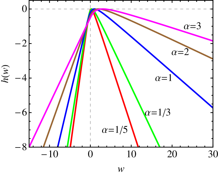
Figure 1: (Color online). Plot of the large deviation function $h(w)$ for $\alpha=1/5$ (red), $1/3$ (green), $1$ (blue), $2$ (brown), and $3$ (magenta).

Let us express the LDF $h(w)$, defined by eq. (6), explicitly in terms of $w$ and $\alpha$. We find that, for $\alpha\leq 1/3$:

$$h(w)=h_{1}(w),$$ (23)

and for $\alpha\geq 1/3$:

$$h(w)=\begin{cases}h_{1}(w)&\text{for}~{}w\geq w^{*}\\ h_{2}(w)&\text{for}~{}w\leq w^{*}\end{cases},$$ (24)

where $h_{1}(w)$ and $h_{2}(w)$ are given by

$$h_{1}(w) =\frac{1}{2}\left[1+w-\sqrt{w^{2}+\alpha}\sqrt{1+\frac{1}{\alpha}}\right],$$ (25)

$$h_{2}(w) =\frac{1-\alpha}{1+\alpha}+\frac{2w}{1+\alpha},$$ (26)

and $w^{*}$ is found by solving $\lambda^{*}(w^{*})=\lambda_{0}$, as

$$w^{*}=\frac{\alpha(\alpha-3)}{3\alpha-1}.$$ (27)

Figure 1 displays the LDF for various $\alpha$.

From the above expressions, it is now straightforward to check the validity of the work SSFT. For $\alpha\leq 1/3$, we get $h(w)-h(-w)=w$, which implies that the SSFT is satisfied. On the other hand, for $1/3<\alpha<3$, we get $h(w)-h(-w)=w$ only for $w^{*}<w<-w^{*}$. For $\alpha\geq 3$, the symmetry relation (7) is not satisfied for any $w$. For example, for $\alpha=3$, we get $w^{*}=0$ and $h(w)-h(-w)=1+w-\sqrt{1+(w^{2}/3)}$ . Figure 2 displays the asymmetry function $\rho(w)\equiv h(w)-h(-w)$ for several values of $\alpha$.

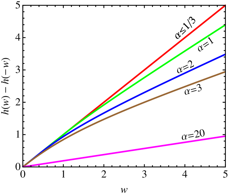
Figure 2: (Color online). Asymmetry function for various $\alpha$.

We can also obtain the the complete asymptotic form of the PDF of the work fluctuations. Skipping details [29], we find that for $\alpha\leq 1/3$:

$$P(W_{\tau}=w\tau/\tau_{\gamma})\approx\frac{K(w)}{2\sqrt{\pi(\tau/\tau_{\gamma})}}\,e^{(\tau/\tau_{\gamma})h_{1}(w)},$$ (28)

and for $\alpha\geq 1/3$:

$$P(W_{\tau}=w\tau/\tau_{\gamma})\approx\, \frac{e^{(\tau/\tau_{\gamma})h_{1}(w)}}{2\sqrt{\pi(\tau/\tau_{\gamma})}}\,\left[K(w)-\frac{\mathrm{sgn}({w^{*}-w})\,g_{-1}}{\sqrt{h_{2}(w)-h_{1}(w)}}\right]$$

$$+e^{(\tau/\tau_{\gamma})h_{2}(w)}\,g_{-1}\left[\frac{\mathrm{sgn}({w^{*}-w})}{2}\,\mathrm{erfc}\Bigl{(}\sqrt{\tau[h_{2}(w)-h_{1}(w)]}\Bigr{)}-\theta(w^{*}-w)\right].$$ (29)

see eq. (29), where

$$K(w) =\alpha^{3/2}(1+1/\alpha)^{3/4}(w^{2}+\alpha)^{-5/4}$$

$$\times\Bigl{[}1+(w+\alpha)\lambda^{*}(w)-h_{1}(w)\Bigr{]}^{-1}$$

$$\times\Bigl{[}\bigl{\{}h_{2}(w)-h_{1}(w)\bigr{\}}+(w-\alpha)\bigl{\{}\lambda^{*}(w)-\lambda_{0}\bigr{\}}\Bigr{]}^{-1},$$ (29)

and

$$g_{-1}=\lim_{\lambda\rightarrow\lambda_{0}}\bigl{[}(\lambda-\lambda_{0})\,g(\lambda)\bigr{]}=-\frac{(3\alpha-1)^{2}}{8\alpha^{2}(1+\alpha)}~{}.$$ (30)

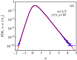
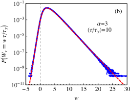
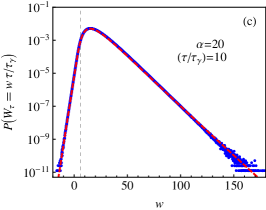
Figure 3: (Color online). $P(W_{\tau})$ against the scaled variable $w=(\tau/\tau_{\gamma})^{-1}W_{\tau}$ for $(\tau/\tau_{\gamma})=10$ and (a) $\alpha=1/3$, (b) $\alpha=3$ and (c) $\alpha=20$ respectively. The points (blue) are obtained from numerical simulation, and the thick dashed lines (red) plot the analytical asymptotic forms given by eq. (28) for (a) and eq. (29) for (b) and (c). The vertical thin dashed lines in (b) and (c) mark the position of $w=w^{*}$.

We compare the above asymptotic forms of the PDF with the results obtained from the numerical simulations of the Langevin equation (2). As seen from fig. 3, the agreements are extremely good, even for $\tau/\tau_{\gamma}=10$.

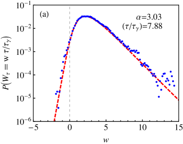
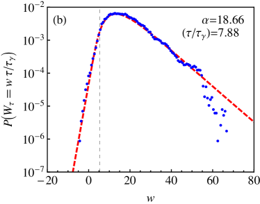
Figure 4: (Color online). $P(W_{\tau})$ against the scaled variable $w=(\tau/\tau_{\gamma})^{-1}W_{\tau}$ for $(\tau/\tau_{\gamma})=7.88\dots$, and (a) $\alpha=3.03$ and (b) $\alpha=18.66$ respectively. The points (blue) are from the micro-cantilever experiment reported in ref. [26], and the thick dashed lines (red) plot the analytical asymptotic form given by eq. (29). The vertical thin dashed lines mark the position of $w=w^{*}$.

We also compare our analytical results against an experiment that was carried out on an atomic-force microscopy cantilever and reported in ref. [26]. The dynamics of the micro-cantilever tip is described by eq. (2) with the viscous relaxation time $\tau_{\gamma}=632\,\mu s$. We find very good agreement between the theory and the experiment, which is shown in fig. 4

So far, we have considered the fluctuations of $W_{\tau}$ in the nonequilibrium steady state, as we have averaged over the initial conditions in eq. (10) with respect to the steady state distribution $\Psi(x_{0},v_{0},0)$ to arrive at eq. (16). Let us now examine how the nature of the initial state affects the results. We recall that the singular part of $g(\lambda)$, i.e., the first factor in eq. (17) comes from the averaging of eq. (10) with respect to the steady state distribution of the initial state. Without the averaging, for any given initial configuration $(x_{0},v_{0})$, the resulting prefactor of $e^{\tau\mu(\lambda)}$ remains analytic throughout the interval $(\lambda_{-},\lambda_{+})$, and hence can be neglected from the saddle point calculation as the subleading contribution. Therefore, the FT for a fixed initial condition is always satisfied, as the LDF is given by eq. (23) for all $\alpha\in(0,\infty)$. If the initial state at $\tau=0$ is chosen from equilibrium —i.e., the average in eq. (10) is taken with respect to the Boltzmann weight $\propto\exp[-E(x_{0},v_{0})/(k_{B}T)]$ — then the first factor in eq. (17) is replaced by $2(1+\alpha)/[1+\eta(\lambda)+2\alpha(1-\lambda)]$. In that case even $g(\lambda)$ satisfies the symmetry relation $g(\lambda)=g(1-\lambda)$. It is easy to see that, now $g(\lambda)$ remains analytic in $(\lambda_{-},\lambda_{+})$ for any $\alpha$. Therefore, the LDF in this case is again given by eq. (23) for all $\alpha\in(0,\infty)$. Consequently, the TFT is satisfied (as $\tau\rightarrow\infty$) for all $\alpha\in(0,\infty)$.

In conclusion, we have studied the work fluctuations of a harmonic oscillator coupled to a thermal bath and driven out of equilibrium by an external Gaussian random force. We have found that the SSFT holds only for weak forcing, whereas the TFT (with $\tau\rightarrow\infty$) holds for all forcing. More importantly, we have analytically obtained the exact LDF as well as the complete asymptotic forms of the PDF of the work fluctuations, and quite interestingly, they are independent of the spring constant of the harmonic oscillator. However, while the LDFs are same for both $k\not=0$ and $k=0$ cases, the complete asymptotic form of the PDFs are different in the two cases. Therefore, $k\rightarrow 0$ limit of PDF (which is anyway independent of $k$) is not same as the PDF in the $k=0$ case. The nature of the work fluctuation is found to be non-Gaussian. These exact results should have broad and important applications, as the harmonic oscillator is ubiquitous in nature. For example, many nanomechanical and biological systems are essentially described by a harmonic oscillator and the results of this Letter are expected to be useful there.

- [1] D. J. Evans, E. G. D. Cohen, and G. P. Morriss, Phys. Rev. Lett. 71, 2401 (1993); D. J. Evans and D. J. Searles, Phys. Rev. E 50, 1645 (1994).
- [2] G. Gallavotti and E. G. D. Cohen, Phys. Rev. Lett. 74, 2694 (1995); J. Stat. Phys. 80, 931 (1995).
- [3] J. Kurchan, J. Phys. A: Math. Gen. 31, 3719 (1998).
- [4] J. L. Lebowitz and H. Spohn, J. Stat. Phys. 95, 333 (1999).
- [5] J. Farago, J. Stat. Phys., 107, 781 (2002).
- [6] R. van Zon and E. G. D. Cohen, Phys. Rev. Lett. 91, 110601 (2003); Phys. Rev. E 67, 046102 (2003); Phys. Rev. E 69, 056121 (2004); R. van Zon, S. Ciliberto, and E. G. D. Cohen, Phys. Rev. Lett. 92, 130601 (2004).
- [7] O. Mazonka and C. Jarzynski, e-print arXiv:cond-mat/9912121; O. Narayan and A. Dhar, J. Phys. A 37, 63 (2004); U. Seifert, Phys. Rev. Lett. 95, 040602 (2005); P. Visco, J. Stat. Mech. (2006) P06006; K. Saito and A. Dhar Phys. Rev. Lett. 99, 180601 (2007); M. Baiesi, T. Jacobs, C. Maes, and N. S. Skantzos, Phys. Rev. E 74, 021111 (2006); R. J. Harris and G. M. Schütz, J. Stat. Mech. (2007) P07020; F. Bonetto, G. Gallavotti, A. Giuliani, and F. Zamponi, J. Stat. Phys 123, 39 (2006).
- [8] C. Jarzynski, Phys. Rev. Lett. 78, 2690 (1997).
- [9] G. E. Crooks, Phys. Rev. E 60, 2721 (1999).
- [10] T. Hatano and S. Sasa, Phys. Rev. Lett. 86, 3463 (2001).
- [11] G. Gallavotti, Phys. Rev. Lett. 77, 4334 (1996).
- [12] G. M. Wang et al., Phys. Rev. Lett. 89, 050601 (2002).
- [13] G. M. Wang et al., Phys. Rev. E 71, 046142 (2005).
- [14] D. M. Carberry et al., Phys. Rev. Lett. 92, 140601 (2004).
- [15] W. I. Goldburg, Y. Y. Goldschmidt, and H. Kellay, Phys. Rev. Lett. 87, 245502 (2001).
- [16] K. Feitosa and N. Menon, Phys. Rev. Lett. 92, 164301 (2004).
- [17] N. Garnier and S. Ciliberto, Phys. Rev. E 71, 060101 (2005).
- [18] J. Liphardt et al., Science 296, 1832 (2002).
- [19] D. Collin et al., Nature 437, 231 (2005).
- [20] S. Majumdar and A. K. Sood, Phys. Rev. Lett. 101, 078301 (2008).
- [21] F. Douarche et al., Phys. Rev. Lett. 97, 140603 (2006).
- [22] N. Kumar, S. Ramaswamy, and A. K. Sood, Phys. Rev. Lett. 106, 118001 (2011).
- [23] E. Falcon et al., Phys. Rev. Lett. 100, 064503 (2008).
- [24] M. Bonaldi et al., Phys. Rev. Lett. 103, 010601 (2009).
- [25] S. Ciliberto, S. Joubaud and A. Petrosyan, J. Stat. Mech. (2010) P12003.
- [26] J. R. Gomez-Solano, L. Bellon, A. Petrosyan and S. Ciliberto, EPL 89, 60003 (2010).
- [27] H. Touchette, Phys. Rep. 478, 1 (2009).
- [28] A. Kundu, S. Sabhapandit and A. Dhar, J. Stat. Mech. (2011) P03007.
- [29] S. Sabhapandit, in preparation (2011).