Energy loss of ions by electric–field fluctuations in a magnetized plasma

Abstract

The results of a theoretical investigation of the energy loss of charged particles in a magnetized classical plasma due to the electric field fluctuations are reported. The energy loss for a test particle is calculated through the linear-response theory. At vanishing magnetic field the electric field fluctuations lead to an energy gain of the charged particle for all velocities. It has been shown that in the presence of strong magnetic field this effect occurs only at low–velocities. In the opposite case of high-velocities the test particle systematically loses its energy due to the interaction with a stochastic electric field. The net effect of the fluctuations is the systematic reduction of the total energy loss (i.e. the sum of the polarization and stochastic energy losses) at vanishing magnetic field and reduction or enhancement at strong field depending on the velocity of the particle. It is found that the energy loss of the slow heavy ion contains an anomalous term which depends logarithmically on the projectile mass. The physical origin of this anomalous term is the coupling between the cyclotron motion of the plasma electrons and the long–wavelength, low–frequency fluctuations produced by the projectile ion. This effect may strongly enhance the stochastic energy gain of the particle.

I Introduction

There is an ongoing interest in the theory of interaction of charged particle beams with plasmas. Although most theoretical works have reported on the energy loss of ions in a plasma without magnetic field, the strongly magnetized case has not yet received as much attention as the field-free case. The energy loss of ion beams and the related processes in magnetized plasmas are important in many areas of physics such as transport, heating, magnetic confinement of thermonuclear plasmas, and astrophysics. Recent applications are the cooling of heavy-ion beams by electrons sor83 ; ner07 ; mol03 and the energy transfer for magnetized target fusion cer00 , or heavy-ion inertial confinement fusion.

For a theoretical description of the energy loss of ions in a plasma, there exist some standard approaches. The dielectric linear response (LR) treatment considers the ion as a perturbation of the target plasma and the stopping is caused by the polarization of the surrounding medium. It is generally valid if the ion couples weakly to the target. Since the early 1960s, a number of calculations of the stopping power within LR treatment in a magnetized plasma have been presented (see Refs. ros60 ; akh61 ; hon63 ; may70 ; ner98 ; ner00 ; ner03 ; ner11 ; see98 ; wal00 ; ste01 ; deu08 and references therein). Alternatively, the stopping is calculated as a result of the energy transfers in successive binary collisions (BCs) between the ion and the electrons ner09 ; zwi99 ; zwi02 ; toe02 . Here it is necessary to consider appropriate approximations for the screening of the Coulomb potential by the plasma ner07 . However, significant gaps between these approaches involve the crucial ion stopping along magnetic field $\mathbf{B}$ and perpendicular to it. In particular, at high $B$ values, the BC predicts a vanishingly parallel energy loss, which remains at variance with the nonzero LR one. Also challenging BC-LR discrepancies persist in the transverse direction, especially for vanishingly small ion projectile velocity $v$ when the friction coefficient contains an anomalous term diverging logarithmically at $v\to 0$ ner00 ; ner03 . For calculation of the energy loss of an ion two new alternative approaches have been recently suggested. One of these methods is specifically aimed at a low-velocity energy loss, which is expressed in terms of velocity–velocity correlation and, hence, to a diffusion coefficient deu08 . Next in Ref. ner11 using the Bhatnagar-Krook-Gross approach based on the Boltzmann-Poisson equations for a collisional and magnetized classical plasma the energy loss of an ion is studied through a LR approach, which is constructed such that it conserves particle local number.

Previous treatments of the energy loss of charged particles in a magnetized plasma ner07 ; mol03 ; cer00 ; ros60 ; akh61 ; hon63 ; may70 ; ner98 ; ner00 ; ner03 ; ner11 ; see98 ; wal00 ; ste01 ; deu08 were obtained by treating the plasma in an average manner, i.e., microscopic fluctuations were neglected. However, any media and, in particular, any plasma being a statistical system, is characterized by stochastic fluctuations. These fluctuations couple to external perturbations and the response of the medium to these perturbations can be expressed through suitable correlation functions of the microscopically fluctuating variables. It is well known that the motion of charged particles in such an environment is stochastic in nature and resembles Brownian motion. The effect of the electromagnetic field fluctuations on the energy loss of a charged particle moving in an unmagnetized classical plasma has been studied by several authors in the past gas65 ; hub61 ; bek66 ; sit67 ; akh75 ; kal61 ; tho60 ; ich73 . This effect leads to an energy gain of the particles and is most effective in the low–velocity limit. In addition the effect of the fluctuations are mainly important for light particles (e.g., for an electron) since this effect is inversely proportional to the mass of the particle and is negligible for heavy ions. Recently similar problem has been formulated for the energy loss in a so–called quark-gluon plasma cha07 which is expected to be formed in relativistic heavy–ion collision experiments. Since the subject of the energy loss is of topical interest, it is the principal motivation of the present paper to quantitatively investigate the effect of microscopic fluctuations on the energy loss of a charged particle passing through an equilibrium, weakly–coupled magnetized plasma. In particular, our main objective is to study through the LR theory the effect of a strong magnetic field on the energy loss process arising due to the fluctuations in a plasma. The sequel is structured as follows. Interactions of a gyrating projectile with target stochastic electric fields are investigated at length in Sec. II. Resulting energy loss rates are respectively explained in Sec. III for a target plasma with no magnetic field and then with an infinite one as well as in Sec. IV for a finite magnetic field and at low–velocity of the particle.

II Interaction of a gyrating particle with plasma stochastic electric field

The dielectric function approach was adopted earlier to calculate the energy loss of charged particles due to polarization effects of the medium ner07 ; mol03 ; cer00 ; ros60 ; akh61 ; hon63 ; may70 ; ner98 ; ner00 ; ner03 ; ner11 ; see98 ; wal00 ; ste01 ; deu08 . It is assumed that the energy lost by the particle is small compared to the energy of the particle itself so that the change in the velocity of the particle during the motion may be neglected, i.e, the particle moves in a straight-line (in $B=0$ case) or helical (in $B\neq 0$ case) trajectory. We consider a nonrelativistic projectile particle with charge $Ze$ ($-e$ is the electron charge) and with a velocity $\mathbf{v}(t)$, which moves in a magnetized classical plasma with a constant magnetic field $\mathbf{B}$. We ignore any role of the electron spin or magnetic moment due to the nonrelativistic motion of the particle and the plasma electrons. The energy loss of a particle is determined by the work of the retarding forces acting on the particle in the plasma from the electric field generated by the particle itself while moving. So the energy loss of the particle per unit time, i.e. energy loss rate (ELR), is given by ner07 ; mol03 ; cer00 ; ros60 ; akh61 ; hon63 ; may70 ; ner98 ; ner00 ; ner03 ; ner11 ; see98 ; wal00 ; ste01 ; deu08

$$\dfrac{dW}{dt}=Ze\mathbf{v}(t)\cdot\mathbf{E}\left(\mathbf{r}(t),t\right),$$ (1)

where the electric field is taken at the location $\mathbf{r}(t)$ of the test particle. Within linear response theory the correlation function of the fluctuations of charge and current densities and the electromagnetic fields in the medium with space-time dispersion are completely determined in terms of the dielectric tensor of the medium. The total electric field $\mathbf{E}(\mathbf{x},t)$ induced in the plasma can be related to the external charge of the test particle by solving Poisson’s equation (see, e.g., Ref. ich73 )

$$\mathbf{E}\left(\mathbf{x},t\right)=-\frac{2iZe}{\left(2\pi\right)^{3}}\int_{-\infty}^{\infty}d\omega\int d\mathbf{k}e^{i\mathbf{k}\cdot\mathbf{x}-i\omega t}\frac{\mathbf{k}}{k^{2}\varepsilon\left(\mathbf{k},\omega\right)}\int_{-\infty}^{\infty}dt^{\prime}e^{i\omega t^{\prime}-i\mathbf{k}\cdot\mathbf{r}(t^{\prime})}.$$ (2)

Here $\varepsilon(\mathbf{k},\omega)=(k_{i}k_{j}/k^{2})\varepsilon_{ij}(\mathbf{k},\omega)$ is the longitudinal dielectric function and $\varepsilon_{ij}(\mathbf{k},\omega)$ is the dielectric tensor of the plasma, respectively.

The previous formula for the energy loss in Eq. (1) does not take into account the fluctuations of the electric fields in the plasma and the particle recoil in interactions. To accommodate these effects it is necessary to replace Eq. (1) with sit67 ; akh75 ,

$$\dfrac{dW}{dt}=Ze\left\langle\mathbf{v}\left(t\right)\cdot\boldsymbol{\mathcal{E}}\left(\mathbf{r}\left(t\right),t\right)\right\rangle,$$ (3)

where $\langle\cdots\rangle$ denotes the statistical averaging operation. It is to be noted that here two averaging procedures are performed: (i) an ensemble average with respect to the equilibrium distribution function and (ii) a time average over random fluctuations in plasma. These two operations are commuting and only after both of them are performed the average quantity takes up a smooth value kal61 . In the following, we will explicitly denote the ensemble average by $\langle\cdots\rangle_{a}$ wherever required to avoid possible confusion.

The electric field $\boldsymbol{\mathcal{E}}(\mathbf{x},t)=\mathbf{E}(\mathbf{x},t)+\tilde{\mathbf{E}}(\mathbf{x},t)$ in Eq. (3) consists of the induced field $\mathbf{E}(\mathbf{x},t)$ given by Eq. (2) and a spontaneously generated microscopic field $\tilde{\mathbf{E}}(\mathbf{x},t)$, the latter being a random function of position and time.

The classical equation of motion of the particle with charge $Ze$ and mass $M$ moving in the fluctuating electric field $\boldsymbol{\mathcal{E}}(\mathbf{x},t)$ and a uniform magnetic field $\mathbf{B}$ have the form

$$\dot{\mathbf{v}}(t)=\varsigma\Omega_{c}\left[\mathbf{v}\left(t\right)\times\mathbf{b}\right]+\frac{Ze}{M}\boldsymbol{\mathcal{E}}\left(\mathbf{r}(t),t\right),$$ (4)

where $\varsigma=|Z|/Z$, $\Omega_{c}=|Z|eB/Mc$ is the cyclotron frequency of the test particle, $\mathbf{b}=\mathbf{B}/B$ is the unit vector along the (external) magnetic field, $\boldsymbol{\mathcal{E}}(\mathbf{x},t)$ is the total electric field involved in Eq. (3), $\mathbf{r}(t)$ is the coordinate of the particle. Note that Eq. (4) is the generalization of the Langevin equation in the presence of a magnetic field where the role of the friction force plays the polarization force determined by a regular electric field $\mathbf{E}(\mathbf{x},t)$ given by Eq. (2).

Introducing the cyclotron rotation matrix $\mathcal{L}_{ij}(t)$ the equation of motion (4) has a formal solution

$$v_{i}\left(t\right)=V_{i}\left(t\right)+\frac{Ze}{M}\int_{-\infty}^{t}dt^{\prime}\mathcal{R}_{ij}\left(t-t^{\prime}\right)\mathcal{E}_{j}\left(\mathbf{r}(t^{\prime}),t^{\prime}\right),$$ (5)

$$x_{i}\left(t\right)=X_{i}\left(t\right)+\frac{Ze}{M\Omega_{c}}\int_{-\infty}^{t}dt^{\prime}\mathcal{L}_{ij}\left(t-t^{\prime}\right)\mathcal{E}_{j}\left(\mathbf{r}(t^{\prime}),t^{\prime}\right),$$ (6)

where $\mathcal{R}_{ij}(t)=(1/\Omega_{c})d\mathcal{L}_{ij}(t)/dt$, $\mathbf{R}(t)$ and $\mathbf{V}(t)$ with the components $X_{i}(t)$ and $V_{i}(t)$, respectively, are the initial (at $t=-\infty$) unperturbed coordinate and velocity of the particle free cyclotron motion, respectively

$$X_{i}\left(t\right)=x_{0i}+\frac{1}{\Omega_{c}}\mathcal{L}_{ij}\left(t\right)v_{0j},$$ (7)

$$V_{i}\left(t\right)=\mathcal{R}_{ij}\left(t\right)v_{0j}.$$

Here the variables $\mathbf{v}_{0}$ and $\mathbf{r}_{0}$ with the components $v_{0i}$ and $x_{0i}$, respectively, are independent and are determined by initial conditions for the free cyclotron motion. Also

$$\mathcal{L}_{ij}\left(t\right)=b_{i}b_{j}\Omega_{c}t+\left(\delta_{ij}-b_{i}b_{j}\right)\sin\left(\Omega_{c}t\right)+\varsigma e_{ijs}b_{s}\left[1-\cos\left(\Omega_{c}t\right)\right],$$ (8)

where $b_{i}$ is the component of the unit vector $\mathbf{b}$ and $e_{ijs}$ is the fully antisymmetrical unit tensor of rank three.

The mean change of the energy of the particle per unit time is given by Eq. (3). The stochastic time dependence as embodied in Eq. (3) comes because of explicit fluctuations in time and motion of the particle from one field point to another. The dependence on the latter will be expanded about the free cyclotron motion where the former will be left untouched. This is done by taking a time interval $\Delta t$ sufficiently large with respect to the time scale of random electric field fluctuations in the plasma ($\tau_{2}$) but small compared with the time during which the particle motion changes appreciably ($\tau_{1}$), $\tau_{2}\ll\Delta t\ll\tau_{1}$. Explicitly, $\tau_{1}\sim[\epsilon^{2}T^{3/2}\ln(1/\epsilon)]^{-1}$ and $\tau_{2}\sim(\epsilon T^{3/2})^{-1}$ kal61 , where $\epsilon=(4\pi n_{e}{\lambda}_{\mathrm{D}}^{3})^{-1}$ is the plasma parameter ($\lambda_{\mathrm{D}}=(T/4\pi n_{e}e^{2})^{1/2}$ and $n_{e}$ are the Debye screening length and electron density, respectively) and $T$ is the plasma temperature measured in energy units. Of course, in the present context of a magnetized plasma the time scales $\tau_{1}$ and $\tau_{2}$ may be strongly modified by the magnetic field, see, e.g., Ref. ner11 . In fact in the Coulomb logarithm determining the time $\tau_{1}$, the Debye length is replaced by the cyclotron radius mon74 . This results in a logarithmic dependence on magnetic field in the relaxation time $\tau_{1}$. On the other hand, at strong magnetic fields $\tau_{2}$ is replaced by the cyclotron period $\tau_{2}\sim\omega^{-1}_{c}$, where $\omega_{c}=eB/mc$ is the cyclotron frequency of the electrons. Thus, independently of the strength of the magnetic field and in the weak coupling limit with $\epsilon\ll 1$, these scales are widely separated. In Eqs. (5) and (6) keeping only the leading order terms in the expansion we obtain

$$v_{i}\left(t\right)=V_{i}\left(t\right)+\frac{Ze}{M}\int_{-\infty}^{t}dt^{\prime}\mathcal{R}_{ij}\left(t-t^{\prime}\right)\mathcal{E}_{j}\left(t^{\prime}\right),$$ (9)

$$\mathcal{E}_{i}\left(\mathbf{r}(t),t\right)=\mathcal{E}_{i}\left(t\right)+\frac{Ze}{M\Omega_{c}}\frac{\partial\mathcal{E}_{i}\left(t\right)}{\partial X_{j}}\int_{-\infty}^{t}dt^{\prime}\mathcal{L}_{js}\left(t-t^{\prime}\right)\mathcal{E}_{s}\left(t^{\prime}\right),$$ (10)

where $\boldsymbol{\mathcal{E}}(t)\equiv\boldsymbol{\mathcal{E}}(\mathbf{R}(t),t)$ and $\mathbf{R}(t)$ is determined by Eq. (7). Substituting Eqs. (9) and (10) into Eq. (3) and neglecting the third order correlations we obtain

$$\dfrac{dW}{dt}=\dfrac{dW_{0}}{dt}+\dfrac{dW_{\mathrm{st}}}{dt},$$ (11)

with

$$\dfrac{dW_{0}}{dt}=Ze\mathbf{V}(t)\cdot\left\langle\boldsymbol{\mathcal{E}}\left(t\right)\right\rangle,$$ (12)

$$\dfrac{dW_{\mathrm{st}}}{dt}=\frac{Z^{2}e^{2}}{M}\left\{\int_{-\infty}^{t}dt^{\prime}\mathcal{R}_{ij}\left(t-t^{\prime}\right)\left\langle\mathcal{E}_{i}\left(t\right)\mathcal{E}_{j}\left(t^{\prime}\right)\right\rangle_{a}+\frac{V_{i}(t)}{\Omega_{c}}\int_{-\infty}^{t}dt^{\prime}\mathcal{L}_{js}\left(t-t^{\prime}\right)\left\langle\frac{\partial\mathcal{E}_{i}\left(t\right)}{\partial X_{j}}\mathcal{E}_{s}\left(t^{\prime}\right)\right\rangle_{a}\right\}.$$ (13)

Because the mean value of the fluctuating part of the electric field equals zero, $\langle\tilde{\mathbf{E}}(\mathbf{x},t)\rangle=0$, $\langle\boldsymbol{\mathcal{E}}\left(t\right)\rangle$ equals the electric field $\mathbf{E}(\mathbf{R}(t),t)$ produced by the particle itself in the plasma. Therefore the first term in Eq. (11) determined by Eq. (12) corresponds to the usual polarization energy loss of the particle calculated for instance in Ref. ner98 for a magnetized plasma. For a gyrating projectile particle Eq. (12) has been evaluated explicitly in Ref. ner98 (see also Ref. ste01 ). Averaging the energy loss $dW_{0}/dt$ with respect to the test particle cyclotron period $2\pi/\Omega_{c}$ (we denote this quantity as $\langle dW_{0}/dt\rangle\equiv S_{0}$) we obtain (see Ref. ner98 for details)

$$S_{0}=\frac{Z^{2}e^{2}}{2\pi^{2}}\sum_{n=-\infty}^{\infty}\int d\mathbf{k}\frac{\zeta_{n}\left(\mathbf{k}\right)}{k^{2}}J_{n}^{2}(k_{\perp}a)\mathrm{Im}\frac{1}{\varepsilon\left(\mathbf{k},\zeta_{n}\left(\mathbf{k}\right)\right)},$$ (14)

where $\zeta_{n}(\mathbf{k})=k_{\parallel}v_{0\parallel}+n\Omega_{c}$, $k_{\parallel}=(\mathbf{k}\cdot\mathbf{b})$, $k_{\perp}^{2}=k^{2}-k_{\parallel}^{2}$, $J_{n}$ is the Bessel function of the $n$th order. Here $v_{0\parallel}$ and $v_{0\perp}\geqslant 0$ are the unperturbed test particle velocities parallel and transverse to the magnetic field direction $\mathbf{b}$, respectively, and $a=v_{0\perp}/\Omega_{c}$ is the cyclotron radius.

Assuming that there exists a hierarchy of scales $\tau_{2}\ll\Delta t\ll\tau_{1}$, it can be shown that the polarization field does not contribute to leading order in the correlations functions appearing in the second term in Eq. (11) as in the case of higher-order Fokker-Planck coefficients hub61 ; ich73 . These terms correspond to the statistical change in the energy of the projectile particle in the plasma due to the fluctuations of the electric field as well as the velocity of the particle under the influence of this field. The first term in Eq. (13) corresponds to the statistical part of the dynamic friction due to the space-time correlation in the fluctuations in the electric field, whereas the second one corresponds to the average change in the energy of the moving particle due to the correlation between the fluctuation in the velocity of the particle and the fluctuation in the electrical field in the plasma. The temporal averaging in Eq. (13), by definition, includes many random fluctuations over the mean cyclotron motion. However, the correlation function of these fluctuations are suppressed beyond their characteristic time scales. This allows us to formally extend the limits in time integrations in Eq. (13) to infinity.

Consider now the energy loss rate (13) of the particle due to the interaction with stochastic plasma electric field. We consider homogeneous plasma and only electrostatic electric fields. In this case the correlation function $\langle\mathcal{E}_{i}(\mathbf{x},t)\mathcal{E}_{j}(\mathbf{x}^{\prime},t^{\prime})\rangle_{a}$ in Eq. (13) is a function of $\mathbf{x}-\mathbf{x}^{\prime}$ and $t-t^{\prime}$. Introducing the power spectrum $P(\mathbf{k},\omega)$ (which is determined by $\langle\mathcal{E}^{2}(\mathbf{x},t)\rangle_{a}$) of the fluctuating electric field this correlation function reads sit67 ; akh75

$$\left\langle\mathcal{E}_{i}\left(\mathbf{x},t\right)\mathcal{E}_{j}\left(\mathbf{x}^{\prime},t^{\prime}\right)\right\rangle_{a}=\int d\mathbf{k}\int_{-\infty}^{\infty}d\omega e^{i\mathbf{k}\cdot(\mathbf{x}-\mathbf{x}^{\prime})-i\omega(t-t^{\prime})}\frac{k_{i}k_{j}}{k^{2}}P\left(\mathbf{k},\omega\right).$$ (15)

Similar expression can be obtained for the correlation function involved in the second term of Eq. (13) and containing the field gradient. Substituting these expressions into Eq. (13) we arrive at

$$\dfrac{dW_{\mathrm{st}}}{dt}=\frac{Z^{2}e^{2}}{M\Omega_{c}}\int\frac{d\mathbf{k}}{k^{2}}\int_{-\infty}^{\infty}d\omega P\left(\mathbf{k},\omega\right)\left(\frac{\partial}{\partial t}+i\omega\right)H\left(\mathbf{k},\omega,t\right),$$ (16)

where

$$H\left(\mathbf{k},\omega,t\right)=\int_{-\infty}^{t}dt^{\prime}\mathcal{L}\left(t-t^{\prime}\right)e^{i\mathbf{k}\cdot(\mathbf{R}(t)-\mathbf{R}(t^{\prime}))-i\omega(t-t^{\prime})},$$ (17)

$$\mathcal{L}\left(t\right)=k_{i}k_{j}\mathcal{L}_{ij}\left(t\right)=k_{\parallel}^{2}\Omega_{c}t+k_{\perp}^{2}\sin\left(\Omega_{c}t\right).$$ (18)

For evaluation of the function $H(\mathbf{k},\omega,t)$ we substitute the unperturbed coordinate (see Eq. (7)) of the free helical motion of the particle into Eq. (17). The time-integration in Eq. (17) can be performed using the Fourier series representation of the exponential function gra80 . After straightforward integration we obtain

$$H\left(\mathbf{k},\omega,t\right)=\sum_{n,l=-\infty}^{\infty}J_{n}\left(k_{\perp}a\right)e^{i\left(n-l\right)\psi}\left\{\frac{-k_{\parallel}^{2}\Omega_{c}}{\left[\omega-\zeta_{l}\left(\mathbf{k}\right)-i0\right]^{2}}J_{l}\left(k_{\perp}a\right)\right.$$ (19)

$$\left.+\frac{k_{\perp}^{2}}{2}\frac{1}{\omega-\zeta_{l}\left(\mathbf{k}\right)-i0}\left[J_{l+1}\left(k_{\perp}a\right)e^{-i\psi}-J_{l-1}\left(k_{\perp}a\right)e^{i\psi}\right]\right\}.$$

Here $\psi=\varsigma(\theta-\varphi)+\Omega_{c}t$, $\varphi$ is the initial phase of the cyclotron motion of the test particle with $v_{0x}=v_{0\perp}\cos\varphi$ and $v_{0y}=v_{0\perp}\sin\varphi$, $\theta$ is the azimuthal angle of the transverse wave vector $\mathbf{k}_{\perp}$ with $k_{x}=k_{\perp}\cos\theta$ and $k_{y}=k_{\perp}\sin\theta$. Next we substitute Eq. (19) into Eq. (16) and average the energy loss rate $dW_{\mathrm{st}}/dt$ with respect to the particle cyclotron period $2\pi/\Omega_{c}$. Then in the term containing $k_{\parallel}^{2}$ performing integrations by parts in the $\omega$-integral, one finally obtains

$$S_{\mathrm{st}}\equiv\left\langle\dfrac{dW_{\mathrm{st}}}{dt}\right\rangle=\frac{\pi Z^{2}e^{2}}{M}\int\frac{d\mathbf{k}}{k^{2}}\int_{-\infty}^{\infty}d\omega\sum_{l=-\infty}^{\infty}\delta\left(\omega-\zeta_{l}\left(\mathbf{k}\right)\right)$$ (20)

$$\times\left\{k_{\parallel}^{2}J_{l}^{2}\left(k_{\perp}a\right)\frac{\partial}{\partial\omega}\left[\omega P\left(\mathbf{k},\omega\right)\right]+\frac{k_{\perp}^{2}}{2\Omega_{c}}\left[J_{l-1}^{2}\left(k_{\perp}a\right)-J_{l+1}^{2}\left(k_{\perp}a\right)\right]\left[\omega P\left(\mathbf{k},\omega\right)\right]\right\}.$$

The above expression is the main result of this paper. For a simplicity we shall call the expression (20) as a Bessel-function representation of the stochastic energy loss rate. For many practical applications, however, it is important to represent the energy loss in an alternative but equivalent integral form, see Appendix A for details. In particular, the integral representation of the energy loss facilitates the limits of a heavy ion (with $M\gg m$, where $m$ is the electron mass) and a weak magnetic field when $\Omega_{c}$ is vanishingly small. Although the stochastic part of the energy loss, Eq. (20), vanishes in the limit $M\to\infty$ for pedagogical purposes we treat this case first keeping the leading term only (proportional to $M^{-1}$). In this case the projectile moves with rectilinear trajectory with an arbitrary angle with respect to the magnetic field. The limit $\Omega_{c}\to 0$ of $S_{\mathrm{st}}$ is performed in Appendix A, see Eq. (49). The second term of this expression contains a full derivative and vanishes after $\omega$-integration and the stochastic energy loss is then given by

$$S_{\mathrm{st}}=\frac{\pi Z^{2}e^{2}}{M}\int_{0}^{2\pi}\frac{d\varphi}{2\pi}\int d\mathbf{k}\left\{\frac{\partial}{\partial\omega}\left[\omega P\left(\mathbf{k},\omega\right)\right]\right\}_{\omega=\mathbf{k}\cdot\mathbf{v}_{0}}.$$ (21)

It should be noted that in Eq. (21) the effect of a magnetic field is contained in the power spectrum $P(\mathbf{k},\omega)$ of the fluctuations. It is seen that formally Eq. (21) is equivalent to the stochastic energy loss derived in Refs. bek66 ; sit67 ; akh75 at vanishing magnetic field assuming that in Eq. (21) $P(\mathbf{k},\omega)$ is the power spectrum at $B=0$ and neglecting the phase average $\int_{0}^{2\pi}d\varphi/2\pi$. In the present context of the magnetized plasma this integration appears due to the average of the energy loss (20) with respect to the cyclotron period $2\pi/\Omega_{c}$ of the particle. Therefore for a conformity of our results with the case of unmagnetized plasma at $B\to 0$ the $\varphi$-average is unnecessary and must be skipped.

It is well known that un upper cutoff parameter $k_{\max}=1/r_{\min}$ (where $r_{\min}$ is the effective minimum impact parameter) must be introduced in Eqs. (14), (20) and (21) to avoid the logarithmic divergence at large $k$. This divergence corresponds to the incapability of the perturbation theory to treat close encounters between the projectile particle and the plasma electrons properly. For $r_{\min}$ we use the effective minimum impact parameter excluding hard Coulomb collisions with a scattering angle larger than $\pi/2$. The resulting cutoff parameter $k_{\max}$ is well known for energy loss calculations (see, e.g., Refs. zwi99 ; ner07 and references therein) and reads $k_{\max}=m(v_{0}^{2}+v_{\mathrm{th}}^{2})/|Z|e^{2}$, where $v_{\mathrm{th}}=(T/m)^{1/2}$ is the thermal velocity of the electrons.

Within linear response theory, the power spectrum $P(\mathbf{k},\omega)$ of the fluctuations of the electrostatic fields at thermal equilibrium follows from the fluctuation-dissipation theorem and is completely determined by the longitudinal dielectric function $\varepsilon(\mathbf{k},\omega)$ of the medium sit67 ; akh75 ,

$$P\left(\mathbf{k},\omega\right)=\frac{4T}{\left(2\pi\right)^{3}\omega}\mathrm{Im}\frac{-1}{\varepsilon\left(\mathbf{k},\omega\right)}.$$ (22)

We consider magnetized electron plasma when the longitudinal dielectric function is given by (see, e.g., Ref. ich73 )

$$\varepsilon\left(\mathbf{k},\omega\right)=1+\frac{1}{k^{2}\lambda_{\mathrm{D}}^{2}}\left\{1+\sum_{n=-\infty}^{\infty}\frac{\omega}{\omega-n\omega_{c}}\Lambda_{n}\left(z\right)\left[W\left(\beta_{n}\right)-1\right]\right\},$$ (23)

where $z=k_{\perp}^{2}a_{e}^{2}$, $\beta_{n}=(\omega-n\omega_{c})/|k_{\parallel}|v_{\mathrm{th}}$, $\Lambda_{n}(z)=e^{-z}I_{n}(z)$, $I_{n}$ is the modified Bessel function of the first kind, $a_{e}=v_{\mathrm{th}}/\omega_{c}$ is the cyclotron radius of the electrons. Also $W(\zeta)=g(\zeta)+if(\zeta)$ is the plasma dispersion function with the real ($g(\zeta)$) and imaginary ($f(\zeta)$) parts fri61

$$g\left(\zeta\right)=1+\frac{\zeta}{\sqrt{2\pi}}\int_{-\infty}^{\infty}\frac{e^{-t^{2}/2}dt}{t-\zeta},\quad f\left(\zeta\right)=\sqrt{\frac{\pi}{2}}\zeta e^{-\zeta^{2}/2}.$$ (24)

In the next sections we consider some particular cases of the stochastic energy loss of the projectile particle, in particular at vanishing and infinitely strong magnetic fields. At vanishing magnetic field we denote the dielectric function as $\varepsilon_{0}(k,\omega)$ which is isotropic and is given by the usual expression (see, e.g., Ref. ich73 )

$$\varepsilon_{0}\left(k,\omega\right)=1+\frac{1}{k^{2}\lambda_{\mathrm{D}}^{2}}W\left(\frac{\omega}{kv_{\mathrm{th}}}\right).$$ (25)

To the dielectric function (25) corresponds the isotropic power spectrum $P_{0}(k,\omega)$ according to Eq. (22). In this case the stochastic energy loss rate (21) is simplified to bek66 ; sit67 ; akh75

$$S_{\mathrm{st}}=\frac{(2\pi)^{2}Z^{2}e^{2}}{M}\int_{0}^{k_{\max}}P_{0}\left(k,kv_{0}\right)k^{2}dk.$$ (26)

At infinitely strong magnetic field we denote the dielectric function as $\varepsilon_{\infty}(\mathbf{k},\omega)$ which is determined by Eq. (25), where, however, the phase velocity $\omega/k$ in the argument of the plasma dispersion function is replaced by $\omega/|k_{\parallel}|$ (see, e.g., Ref. ner07 ).

The above expressions gives the mean energy (per unit time) absorbed (or emitted) by a propagating projectile particle from the heat reservoir. Physically, this arises from the energy absorption from thermal fluctuations. In the absence of the magnetic field it is to be noted here that because the spectral density $P_{0}(k,\omega)$ of the fluctuations of the electric fields is positive for positive frequencies by definition, according to Eq. (26) the particle energy will grow due to interactions with the fluctuating electric fields. The present situation with a magnetized plasma may be quit different. It will be further discussed in Sec. III.

III ELR without and with strong magnetic field

To illustrate the problem of the stochastic energy loss and the interrelation of the treatments determined by Eqs. (14) and (20), we consider the cases without and with an infinitely strong magnetic field. In the absence of a magnetic field the interaction of the test particle with stochastic plasma electric fields yields a positive ELR (which corresponds to an energy gain by the particle) and the total ELR decreases. At strong magnetic field, however, the stochastic interaction of the projectile may result in positive or negative ELR depending on the velocity of the particle.

III.1 ELRs at vanishing magnetic field

For a vanishing magnetic field when $a_{e}\gg\lambda_{\mathrm{D}}$ (or $\omega_{c}\ll\omega_{p}$), the power spectrum of the fluctuation of the plasma electric fields is determined by Eq. (22), where the longitudinal dielectric function is given by the field-free expression (25). At vanishing magnetic field the ELRs $S_{0}$ and $S_{\mathrm{st}}$ have been evaluated previously in Refs. deu86 ; pet91 and bek66 ; sit67 ; akh75 (see also references therein), respectively. In the leading order with respect to the cutoff parameter $k_{\max}$ the ELRs $S_{0}$ and $S_{\mathrm{st}}$ read

$$S_{0}=-Q_{0}\frac{\pi}{\lambda}\left\{\ln\xi\left[\mathrm{erf}\left(\frac{\lambda}{\sqrt{2}}\right)-\frac{2}{\pi}f\left(\lambda\right)\right]-\frac{2}{\pi}\int_{0}^{\lambda}\Xi\left(u\right)udu\right\},$$ (27)

$$S_{\mathrm{st}}=Q_{0}\frac{m}{M}\frac{2}{\lambda}\left[f\left(\lambda\right)\ln\xi-\Xi\left(\lambda\right)\right],$$ (28)

where $\mathrm{erf}(z)$ is the error function, $Q_{0}=4n_{e}Z^{2}e^{4}/mv_{\mathrm{th}}$, $\xi=k_{\max}\lambda_{\mathrm{D}}=(\lambda^{2}+1)/\epsilon|Z|$, $\lambda=v_{0}/v_{\mathrm{th}}$ is the projectile velocity in units of thermal velocity. Also

$$\Xi\left(u\right)=\frac{1}{4}f\left(u\right)\ln\left[g^{2}\left(u\right)+f^{2}\left(u\right)\right]+\frac{1}{2}g\left(u\right)\left[\frac{\pi}{2}-\arctan\frac{g\left(u\right)}{f\left(u\right)}\right].$$ (29)

It is well known that at vanishing magnetic field the ELRs determined by $S_{0}$ and $S_{\mathrm{st}}$ are always negative and positive, respectively. This features correspond to the energy loss and energy gain, respectively, by projectile particle.

Consider briefly some limiting cases for the low- and high-velocity projectiles. Taking into account the behavior of the function $\Xi(u)\simeq(1/2)\sqrt{\pi/2}u$ (at $u\ll 1$) and $\Xi(u)\simeq-\pi/2u^{2}$ (at $u\gg 1$), at low- ($\lambda\ll 1$) and high-velocities ($\lambda\gg 1$) the ELRs become

$$S_{0}\simeq-Q_{0}\frac{\sqrt{2\pi}}{3}\lambda^{2}\left(\ln\frac{1}{\epsilon|Z|}-\frac{1}{2}\right),\quad S_{\mathrm{st}}\simeq Q_{0}\frac{m}{M}\sqrt{2\pi}\left(\ln\frac{1}{\epsilon|Z|}-\frac{1}{2}\right),$$ (30)

$$S_{0}\simeq-Q_{0}\frac{\pi}{\lambda}\ln\left(\frac{\lambda^{3}}{\epsilon|Z|}\right),\quad S_{\mathrm{st}}\simeq Q_{0}\frac{m}{M}\frac{\pi}{\lambda^{3}},$$ (31)

respectively. For derivation of the first relation in Eq. (31) we have used the frequency sum rule for the dielectric function (25). From Eqs. (30) and (31) it is seen that for light projectile particle (for instance for an electron with $M=m$) the stochastic ELR may essentially contribute to the total energy loss at small velocities. Then the total rate $S_{0}+S_{\mathrm{st}}$ becomes positive which corresponds to an energy gain by projectile particle. At high-velocities, however, the ELR $S_{0}$ essentially exceeds the stochastic energy loss and the total ELR remains negative.

III.2 ELRs at infinitely strong magnetic field

We now turn to the case when a projectile particle moves in a plasma with a strong magnetic field, which is, on one hand, sufficiently weak to allow a classical description ($\hbar\omega_{c}<T$), and, on the other hand, comparatively strong so that the cyclotron frequency of the plasma electrons exceeds the plasma frequency $\omega_{c}\gg\omega_{p}$ (or $a_{e}\ll\lambda_{\mathrm{D}}$). This limits the values of the magnetic field, the temperature, and the plasma density. From these conditions we can obtain $3\times 10^{-6}\sqrt{n_{e}}<B<10^{5}T$, where $n_{e}$ is measured in cm^-3, $T$ in eV, and $B$ in kG. The plasma electrons in the lowest order can respond to the excited waves only in the direction of $\mathbf{B}$. Because of this assumption, the perpendicular cyclotron motion of the test and plasma particles is neglected. As shown by Rostoker and Rosenbluth ros60 the plasma waves involved in this case are oblique plasma waves having the approximate dispersion relation $\omega=\omega_{p}k_{\parallel}/k$.

The dielectric function $\varepsilon_{\infty}(\mathbf{k},\omega)$ is obtained from Eq. (25), where, however, the phase velocity $\omega/k$ in the argument of the plasma dispersion function is replaced by $\omega/|k_{\parallel}|$. The corresponding power spectrum of the fluctuations in the presence of strong magnetic field is connected to $\varepsilon_{\infty}(\mathbf{k},\omega)$ via relation (22). Neglecting the transversal cyclotron motion of the test particle and the electrons in Eqs. (14) and (20) in the lowest order one obtains (see, e.g., Ref. ner98 ; ner07 )

$$S_{0}=-Q_{0}\lambda\left[f\left(\lambda\right)\ln\xi-\Xi\left(\lambda\right)\right],$$ (32)

$$S_{\mathrm{st}}=\frac{\pi Z^{2}e^{2}}{M}\int d\mathbf{k}\frac{k_{\parallel}^{2}}{k^{2}}\frac{\partial}{\partial\omega}\left[\omega P\left(\mathbf{k},\omega\right)\right]_{\omega=k_{\parallel}v_{0\parallel}},$$ (33)

where now $\lambda=v_{0\parallel}/v_{\mathrm{th}}$. Substituting the power spectrum of the fluctuations with the dielectric function $\varepsilon_{\infty}(\mathbf{k},\omega)$ in Eq. (33) in the leading order with respect to the cutoff parameter $\xi$ we arrive at

$$S_{\mathrm{st}}=Q_{0}\frac{m}{M}\frac{\partial}{\partial\lambda}\left[f\left(\lambda\right)\ln\xi-\Xi\left(\lambda\right)\right],$$ (34)

where $\Xi(\lambda)$ is determined by Eq. (29).

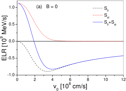
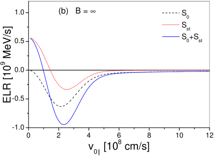
Figure 1: (Color online) Electron energy loss rate (in units of $10^{9}$ MeV/s) in a plasma with $n_{e}=10^{20}$ cm^-3, $T=10$ eV ($\epsilon=0.06$) in terms of the velocity (in units of $10^{8}$ cm/s) at vanishing (a) and strong (b) magnetic field. The energy loss rates $S_{0}$ and $S_{\mathrm{st}}$ and the total rate $S_{0}+S_{\mathrm{st}}$ are shown as dashed, dotted and solid lines, respectively.

Consider briefly the limits of low- and high-velocities. At $\lambda\ll 1$ from Eqs. (32) and (34) one obtains

$$S_{0}\simeq-Q_{0}\sqrt{\frac{\pi}{2}}\lambda^{2}\left(\ln\frac{1}{\epsilon|Z|}-\frac{1}{2}\right),$$ (35)

$$S_{\mathrm{st}}\simeq Q_{0}\frac{m}{M}\sqrt{\frac{\pi}{2}}\left(\ln\frac{1}{\epsilon|Z|}-\frac{1}{2}\right).$$ (36)

At high-velocities, $\lambda\gg 1$, Eqs. (32) and (34) become

$$S_{0}\simeq-Q_{0}\frac{\pi}{2\lambda},\quad S_{\mathrm{st}}\simeq-Q_{0}\frac{m}{M}\frac{\pi}{\lambda^{3}},$$ (37)

respectively. It is seen that unlike the field-free case where the energy loss rate $S_{\mathrm{st}}$ in Eqs. (30) and (31) is always positive, the ELR in the presence of a strong magnetic field is positive at small-velocities while it is negative at high-velocities. For a light particle (e.g. for an electron) the stochastic ELR even essentially exceeds the energy loss $S_{0}$ at small velocity limit and the total ELR becomes positive. The results of the numerical evaluation of Eqs. (27), (28) and (32), (34) are shown in Fig. 1 for an electron test particle ($M=m$) moving in a plasma with $n_{e}=10^{20}$ cm^-3 and $T=10$ eV ($\epsilon=0.06$). This figure shows the ELR (in units of $10^{9}$ MeV/s) as a function of the particle velocity (in units of $10^{8}$ cm/s) at vanishing (left panel) and at strong (right panel) magnetic field. It is evident that the effect of the electric field fluctuations on the test particle energy loss is significant at low-velocities both for vanishing and strong magnetic field. At higher velocities the relative importance of the stochastic energy loss to the usual energy loss $S_{0}$ decreases gradually. We also mention that similar calculation can be done for any test ion with $M\gg m$. However, the stochastic energy loss for an ion both at vanishing and infinitely strong magnetic field at least three orders of magnitude smaller than $S_{\mathrm{st}}$ shown in Fig. 1.

We would like to close this section with the following remark. From Eqs. (30) and (36) it is seen that the fluctuation energy loss rate does not vanish at low-velocities (as it occurs with the polarization energy loss rates (30) and (35)) for vanishing and strong magnetic field and the corresponding friction coefficient diverges as $v_{0}\to 0$. For arbitrary magnetic field similar conclusion can be made on the basis of a general expression (48) where the stochastic ELR is given in the integral representation. At the vanishing ion velocity (i.e. at $v_{0}\to 0$) this expression yields

$$S_{\mathrm{st}}=\frac{\pi Z^{2}e^{2}}{M}\int\frac{d\mathbf{k}}{k^{2}}\left[k_{\parallel}^{2}P\left(\mathbf{k},0\right)+k_{\perp}^{2}P\left(\mathbf{k},\Omega_{c}\right)\right].$$ (38)

It is seen that in low–velocity limit and for arbitrary $B$ the rate $S_{\mathrm{st}}$ is finite and its longitudinal and transversal parts are determined by static $P(\mathbf{k},0)$ and dynamic $P(\mathbf{k},\Omega_{c})$ fluctuation spectra, respectively. At vanishing magnetic field (i.e. at $\Omega_{c}\to 0$) the second term in Eq. (38) can be collected with the first one and the resulting ELR coincides with Eq. (26) in the limit $v_{0}\to 0$. In this case the stochastic energy loss is only determined by the static fluctuation spectra $P(k,0)$. This feature of the stochastic ELR at vanishing velocity is closely resembled the Brownian motion. In fact at $Mv^{2}/2\lesssim T$ when the kinetic energy of the particle is comparable with the thermal energy of the plasma environment the particle motion is stochastic in nature. The energy change of the particle is determined by the correlation function $C(t)=\langle\mathbf{v}_{\mathrm{st}}(t)\cdot\mathbf{F}_{\mathrm{st}}(t)\rangle$, where $\mathbf{F}_{\mathrm{st}}(t)$ is the stochastic force acting on the particle and $\mathbf{v}_{\mathrm{st}}(t)$ is the stochastic velocity of the particle under the influence of $\mathbf{F}_{\mathrm{st}}(t)$. At low velocities $\mathbf{v}_{\mathrm{st}}(t)$ can be estimated employing the Langevin equation and the result at long times reads $\mathbf{v}_{\mathrm{st}}(t)\simeq(1/\gamma M)\mathbf{F}_{\mathrm{st}}(t)$, where $\gamma$ is the friction coefficient. Thus, asymptotically $C(t)\simeq(1/\gamma M)\langle\mathbf{F}^{2}_{\mathrm{st}}(t)\rangle$ is a constant at thermal equilibrium which is determined by the thermodynamic properties of the medium. At vanishing magnetic field this constant is related to the static fluctuation spectrum $P(k,0)$ while in $B\neq 0$ case the fluctuations give rise the cyclotron motion of the particle and the transversal part of $C(t)$ is determined by the dynamic spectrum $P(\mathbf{k},\Omega_{c})$, see the second term in Eq. (38).

IV ELR at low–velocities and for intermediate magnetic field

In Sec. III, the effect of the electric–field fluctuations on the energy loss of the projectile particle has been investigated in two extreme regimes with vanishing and very strong magnetic fields. In this section we extend these results considering briefly some intermediate cases with finite magnetic field which cover the entire domain between field–free and strong magnetic field regimes. As will be shown below at $a_{e}\sim\lambda_{\mathrm{D}}$ the effect of the magnetic field on the energy loss process shows some additional features. In general, the analytical or numerical investigation of the energy loss rates given by Eqs. (14) and (20) with Eqs. (22) and (23) for arbitrary $B$ and the test particle velocity $v$ is a formidable task and requires separate investigations. Previously the energy loss $S_{0}$ has been investigated numerically and analytically for arbitrary $B$ and $v$ but mostly neglecting the gyration of the test particle, Refs. ner07 ; mol03 ; cer00 ; ros60 ; akh61 ; hon63 ; may70 ; ner98 ; ner00 ; ner03 ; ner11 ; see98 ; wal00 ; ste01 ; deu08 . To gain more insight into the magnetic field effect on the stochastic energy loss process we consider here the limit of low–velocity projectile ion when electric field fluctuations are expected to be very important. In this case assuming a heavy ion ($M\gg m$) the imaginary part of the inverse dielectric function (spectral function) involved in Eq. (22) is represented in the form

$$\mathrm{Im}\frac{-1}{\varepsilon\left(\mathbf{k},\omega\right)}=\frac{\mathrm{Im}\left[\varepsilon\left(\mathbf{k},\omega\right)\right]}{\left|\varepsilon\left(\mathbf{k},\omega\right)\right|^{2}}\simeq\frac{\mathrm{Im}\left[\varepsilon\left(\mathbf{k},\omega\right)\right]}{\left|\varepsilon\left(\mathbf{k},0\right)\right|^{2}}.$$ (39)

Note that in the last part of Eq. (39) the dynamical screening has been replaced by the static one thus neglecting the collective plasma resonances involved in $\varepsilon(\mathbf{k},\omega)$. For arbitrary velocities this simplified version of the spectral function and the corresponding ELR has been calculated in Refs. ner03 ; ner07 with vanishing and strong magnetic fields. It has been shown that at $B=0$ the simplified and the full spectral functions yield close ELRs at low–velocities. However, at $v_{0}>v_{\mathrm{th}}$ when the collective effects play an important role these approaches deviate from each other. On the other hand, the strong magnetic field reduces the transversal dynamics of the plasma electrons and the role of the collective effects becomes less important which results in the good agreement between two approaches in a whole velocity range.

Consider the ELR $S_{0}$ given by Eq. (14) assuming that the projectile ion moves along the magnetic field (i.e $v_{0\perp}=0$) with $v_{0\parallel}=v_{0}\ll v_{\mathrm{th}}$. Inserting the approximate spectral function (39) into Eq. (14) and introducing new integration variables $\kappa=k^{2}a^{2}_{e}$, $\mu=\cos^{2}\theta$ (where $\theta$ is the angle between $\mathbf{k}$ and $\mathbf{B}$) we arrive at

$$S_{0}\simeq-\sqrt{\frac{\pi}{8}}Q_{0}\lambda^{2}\int_{0}^{\eta^{2}\xi^{2}}\frac{\kappa d\kappa}{\left(\kappa+\eta^{2}\right)^{2}}\int_{0}^{1}d\mu\sum_{n=-\infty}^{\infty}\Lambda_{n}\left(\kappa\left(1-\mu\right)\right)\exp\left(-\frac{n^{2}}{2\kappa\mu}\right),$$ (40)

where $\lambda=v_{0}/v_{\mathrm{th}}$, $\eta=a_{e}/\lambda_{\mathrm{D}}$, and the other quantities have been introduced in Secs. II and III.

The stochastic ELR at low–velocities is determined by Eq. (38) where the first and the second terms are the contributions from longitudinal and transversal fluctuations, respectively. It should be emphasized that the relation (39) is justified for the first term of Eq. (38) where only the static spectrum $P(\mathbf{k},0)$ is involved. The second term contains the cyclotron frequency $\Omega_{c}$ of the projectile ion. Since $\Omega_{c}\ll\omega_{c}$ the ion cannot resonate with plasma electron resonances involved in the dielectric function and in the fluctuation spectrum $P(\mathbf{k},\Omega_{c})$ the simplification given by Eq. (39) is again justified.

Consider now Eq. (38) with Eqs. (22) and (39). Using the integration variables introduced above we obtain

$$S_{\mathrm{st}}\simeq\sqrt{\frac{\pi}{8}}\frac{m}{M}Q_{0}\int_{0}^{\eta^{2}\xi^{2}}\frac{\kappa d\kappa}{\left(\kappa+\eta^{2}\right)^{2}}\int_{0}^{1}\frac{d\mu}{\mu}\sum_{n=-\infty}^{\infty}\Lambda_{n}\left(\kappa\left(1-\mu\right)\right)$$ (41)

$$\times\left\{\mu\exp\left(-\frac{n^{2}}{2\kappa\mu}\right)+\left(1-\mu\right)\exp\left[-\frac{\left(n-\alpha\right)^{2}}{2\kappa\mu}\right]\right\},$$

where $\alpha=|Z|m/M\ll 1$. Let us recall that at low–velocities the ELR, $S_{\mathrm{st}}$, in the leading order does not depend on the ion velocity while $S_{0}\sim\lambda^{2}$ (see Eq. (40)). It is seen that the term of Eq. (41) with $n=0$ (no cyclotron motion) exhibits a singular behavior in the limit of $\alpha\ll 1$ where the $\mu$ integration diverges logarithmically for small $\mu$ (or small $k_{\parallel}$). We must therefore keep $\alpha$ finite in that integration to avoid such a divergence. This anomalous contribution that arises from the term of Eq. (41) with $n=0$ is denoted as $S_{\mathrm{st}}^{\prime}$. The other terms of Eq. (41) with $n\neq 0$ do not exhibit singular behavior at $\alpha\ll 1$ and their contribution to the stochastic energy loss is denoted as $S_{\mathrm{st}}^{\prime\prime}$ ($S_{\mathrm{st}}=S_{\mathrm{st}}^{\prime}+S_{\mathrm{st}}^{\prime\prime}$). Thus in the limit of a heavy projectile ion with $\alpha\ll 1$ from Eq. (41) in the leading order we obtain

$$S_{\mathrm{st}}^{\prime}=\sqrt{\frac{\pi}{8}}\frac{m}{M}Q_{0}\int_{0}^{\eta^{2}\xi^{2}}\frac{\kappa d\kappa}{\left(\kappa+\eta^{2}\right)^{2}}\left\{\Lambda_{0}\left(\kappa\right)\left(\ln\frac{2\kappa}{\alpha^{2}}-\gamma\right)\right.$$ (42)

$$\left.+\int_{0}^{1}\left[\Lambda_{0}\left(\kappa\left(1-\mu\right)\right)-\Lambda_{0}\left(\kappa\right)\right]\frac{d\mu}{\mu}\right\},$$

$$S_{\mathrm{st}}^{\prime\prime}=\sqrt{\frac{\pi}{2}}\frac{m}{M}Q_{0}\int_{0}^{\eta^{2}\xi^{2}}\frac{\kappa d\kappa}{\left(\kappa+\eta^{2}\right)^{2}}\int_{0}^{1}\frac{d\mu}{\mu}\sum_{n=1}^{\infty}\Lambda_{n}\left(\kappa\left(1-\mu\right)\right)\exp\left(-\frac{n^{2}}{2\kappa\mu}\right),$$ (43)

where $\gamma=0.5772\ldots$ is the Euler’s constant. The terms neglected in deriving Eqs. (42) and (43) are of the order of $\mathrm{O}(\alpha^{2})$ and $\mathrm{O}(\alpha^{2}\ln\alpha)$. Also we note that the anomalous ELR $S_{\mathrm{st}}^{\prime}$ given by Eq. (42) is valid at $\alpha<\eta$ (or $\Omega_{c}<\omega_{p}$) which is easily fulfilled for heavy ions. In the opposite case with $\alpha>\eta$ (but $\alpha\ll 1$) one should consider more general Eq. (41) as a starting point for investigation of the anomalous ELR.

The ELR (42) can be further simplified assuming that $\eta>1/\xi$ (or $a_{e}>r_{\min}$). This condition allows one to extend the upper limit of the integration in Eq. (42) to infinity which yields

$$S_{\mathrm{st}}^{\prime}\simeq\sqrt{\frac{\pi}{8}}\frac{m}{M}Q_{0}\left[\left(\ln\frac{2}{\alpha^{2}}-\gamma-1\right)G_{0}\left(\eta^{2}\right)+G_{1}\left(\eta^{2}\right)\right]$$ (44)

where

$$G_{0}\left(x\right)=\int_{0}^{\infty}\frac{\Lambda_{0}\left(\kappa\right)\kappa d\kappa}{\left(\kappa+x\right)^{2}}=e^{x}\left[\left(1+x\right)K_{0}\left(x\right)-xK_{1}\left(x\right)\right],$$ (45)

$$G_{1}\left(x\right)=\int_{0}^{\infty}\ln\left(\kappa+x\right)\frac{\Lambda_{0}\left(\kappa\right)\kappa d\kappa}{\left(\kappa+x\right)^{2}}.$$ (46)

Here $K_{0}(x)$ and $K_{1}(x)$ are the modified Bessel functions of the second kind. The integral involved in the function $G_{0}(x)$ has been evaluated by Ichimaru (see Ref. ich73 for details).

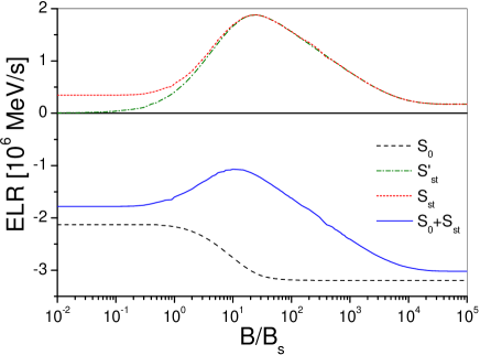
Figure 2: (Color online) Proton energy loss rate (in units of $10^{6}$ MeV/s) in a plasma with $n_{e}=10^{20}$ cm^-3, $T=10$ eV ($\epsilon=0.06$) vs scaled magnetic field $B/B_{s}$ and at low–velocities ($\lambda=0.1$). The energy loss rates $S_{0}$, $S^{\prime}_{\mathrm{st}}$ and $S_{\mathrm{st}}$ and the total rate $S_{0}+S_{\mathrm{st}}$ are shown as dashed, dot–dashed, dotted and solid lines, respectively. See the text for explanations.

Consider briefly the connection of Eqs. (40)–(44) to the ELRs obtained in the previous section for two limiting cases. It is seen from Eqs. (40) and (41) that at very strong magnetic field only the terms with $n=0$ contribute to the ELRs. Then the ELRs (40) and (41) in the limit of $\eta\to 0$ after $\kappa$ integration coincide with Eqs. (35) and (36), respectively. We merely note that in this limit the ELR $S_{\mathrm{st}}^{\prime\prime}$ vanishes and the stochastic energy loss in the case of very strong magnetic field is determined by the anomalous term $S_{\mathrm{st}}^{\prime}$.

Next we treat the limit of the vanishing magnetic field ($\eta\to\infty$). In this case all cyclotron harmonics in Eqs. (40) and (41) contribute to the ELRs. It is useful to transform the $n$ summations in these expressions into an integral form where the limit $\eta\to\infty$ can be easily done. Since this procedure is similar to one considered in Appendix A we refer a reader to Refs. ner07 ; ner11 for more details. As a result we obtain that at vanishing magnetic field the $n$ summation in Eq. (40) is replaced by $\sqrt{\mu}$. The remaining integrals can be easily performed. After evaluating these integrals one can see that the ELR $S_{0}$ at $\eta\to\infty$ completely agrees with the first relation in Eq. (30). We turn now to the anomalous term given by Eq. (44). Using the asymptotic behavior of the modified Bessel functions one cane see that the functions $G_{0}(\eta^{2})$ and $G_{1}(\eta^{2})$ at $\eta\to\infty$ behave as $\sim 1/\eta$ and $\sim(1/\eta)\ln\eta$, respectively, and thus vanish in the field–free case. On the other hand the stochastic ELR $S_{\mathrm{st}}^{\prime\prime}$ is evaluated in a same manner as explained above and the summation in Eq. (43) in a limit of vanishing magnetic field yields $\sqrt{\mu}/2$. Substituting this formula into Eq. (43) and performing $\mu$ and $\kappa$ integrations we finally arrive at the second relation of Eq. (30). The anomalous term Eqs. (42) and (44) therefore represent a new effect arising from the presence of the magnetic field. The physical origin of such an anomalous ELR is the same as those obtained in Ref. ich73 and Refs. ner07 ; ner00 for the transport coefficients and the stopping power of an ion, respectively. It may be traced to the spiral motion of the electrons along the magnetic field lines. These electrons naturally tend to couple strongly with long-wavelength fluctuations (i.e., small $k_{\parallel}$) along the magnetic field. In addition, when such fluctuations are characterized by slow variation in time (i.e., small $\omega=\Omega_{c}$), the contact time or the rate of energy exchange between the electrons and the fluctuations will be further enhanced. In a plasma, such low–frequency fluctuations are provided by the slow projectile ion. The above coupling can therefore be an efficient mechanism of energy exchange between the electrons and the projectile ion. In the limit of $\Omega_{c}\to 0$ (or $M\to\infty$), the contact time thus becomes infinite and the ELR diverges.

In the presence of strong magnetic field one could expect that for heavy ions the anomalous ELR $S^{\prime}_{\mathrm{st}}$ mainly contributes to the total stochastic ELR $S_{\mathrm{st}}$. To demonstrate this feature the ELRs are plotted in Fig. 2 vs scaled magnetic field $B/B_{s}$ for $v_{0}=0.1v_{\mathrm{th}}\simeq 1.3\times 10^{7}$ cm/s, $n_{e}=10^{20}$ cm^-3, $T=10$ eV, where $B_{s}=mc\omega_{p}/e\simeq 3.2\times 10^{4}$ kG. The energy loss rates $S_{0}$, $S^{\prime}_{\mathrm{st}}$ and $S_{\mathrm{st}}$ and the total rate $S_{0}+S_{\mathrm{st}}$ are found for a proton projectile and are shown as dashed, dot–dashed, dotted and solid lines, respectively. In Fig. 2 the limiting cases of the vanishing and very strong magnetic fields considered in Sec. III are reached at $B\lesssim B_{s}$ and $B\gtrsim 10^{4}B_{s}$, respectively. It is seen that the magnetic field may essentially increase the ELRs in plasma compared to the field–free (Eq. (30)) and strong field (Eqs. (35) and (36)) regimes and this occurs at $B\gtrsim 10B_{s}$. In the latter case the stochastic ELR is mainly determined by the anomalous ELR $S^{\prime}_{\mathrm{st}}$. Furthermore, at low ion velocities the fluctuations in the electric field essentially counter the effect of the polarization field resulting in the reduced ELR (solid line in Fig. 2).

As discussed above, Eqs. (40) and (41) and hence the results shown in Fig. 2 account for only static screening neglecting dynamic polarization effects. As shown in Refs. ner07 ; ner03 in a vanishing or very strong magnetic field these effects are not important at low–velocities, and the situation with finite $B$ requires further investigations, in particular for electron projectiles. Intuitively it is clear that a gyrating test electron may resonate with a electron plasma fluctuations with a cyclotron frequency $\omega_{c}$, and the approximation (39) is not as obvious as for the case of a heavy ion. Also it should be emphasized that the validity of the regime of a classically strong magnetic field requires the condition $B<B_{c}=(mc/e\hslash)T$. Thus the results shown in Fig. 2 are valid up to $B_{c}/B_{s}=T/\hslash\omega_{p}\simeq 27$. Clearly the realization of the regime of a strong magnetic field requires high temperatures and low densities and the enhancement of the ELRs at $B\gtrsim 10B_{s}$ may not be accessible under certain conditions.

V Summary

In this paper within linear response theory we have investigated the energy loss rate (ELR) of a nonrelativistic projectile particle moving in a magnetized classical plasma due to the electric field fluctuations. In the course of this study we have derived general expression for the stochastic energy loss rate. As in the field–free case the later is completely determined by the fluctuation power spectrum $P(\mathbf{k},\omega)$. Assuming an equilibrated and homogeneous magnetized plasma when the power spectrum of the fluctuations is derived from the fluctuation–dissipation theorem and is expressed via longitudinal dielectric function of the medium we have considered two somewhat distinct cases with vanishing and with extremely strong magnetic field. At vanishing magnetic field the electric field fluctuations lead to an energy gain of the charged particle for all velocities. Physically, this is arisen due to the energy absorption by projectile particle from thermal fluctuations. It has been shown that in the presence of strong magnetic field this effect occurs only at low–velocities. At high–velocities the test particle systematically loses its energy due to the interaction with a stochastic electric field.

In the low–velocity limit but for arbitrary magnetic field, we have found an enhanced stochastic ELR of an ion compared to the limiting cases with vanishing and very strong magnetic fields, mainly due to the strong coupling between the spiral motion of the electrons and the long–wavelength, low–frequency fluctuations excited by the projectile. The nature of this anomalous ELR is only conditioned by the external magnetic field.

The analysis presented above can in principle be extended to the case of a nonequilibrium magnetized plasma, provided the power spectrum of the electrostatic fluctuations are known. In principle the power spectrum can be derived within linear response theory sit67 ; akh75 . Fluctuations are much stronger in nonequilibrium situations than in systems in thermal equilibrium sit67 ; akh75 . The effect of the electric field fluctuations on the particle energy loss is therefore expected to be stronger in a nonequilibrium plasma. We intend to address this issue in our forthcoming investigations.

Appendix A Integral representation of the stochastic energy loss

In Sec. II we have derived the Bessel-function representation of the stochastic energy loss of a gyrating test particle. For some applications an integral representation of $S_{\mathrm{st}}$ is desirable. For deriving the integral form of the energy loss we rewrite the delta-function $\delta(\omega-\zeta_{l}(\mathbf{k}))$ in Eq. (20) using an integral representation of this function. Then Eq. (20) becomes

$$S_{\mathrm{st}}=\frac{Z^{2}e^{2}}{2M}\int\frac{d\mathbf{k}}{k^{2}}\int_{-\infty}^{\infty}d\omega\int_{-\infty}^{\infty}dte^{i(\omega-k_{\parallel}v_{0\parallel})t}\sum_{l=-\infty}^{\infty}e^{-il\Omega_{c}t}J_{l}^{2}\left(k_{\perp}a\right)$$ (47)

$$\times\left\{k_{\parallel}^{2}\frac{\partial}{\partial\omega}\left[\omega P\left(\mathbf{k},\omega\right)\right]-ik_{\perp}^{2}\frac{\sin\left(\Omega_{c}t\right)}{\Omega_{c}}\left[\omega P\left(\mathbf{k},\omega\right)\right]\right\}.$$

Then using the summation formula $\sum_{l=-\infty}^{\infty}e^{ilt}J_{l}^{2}(z)=J_{0}(2z\sin\frac{t}{2})$ gra80 the stochastic energy loss may be alternatively represented in the form

$$S_{\mathrm{st}}=\frac{Z^{2}e^{2}}{M}\int\frac{d\mathbf{k}}{k^{2}}\int_{-\infty}^{\infty}d\omega\int_{0}^{\infty}J_{0}\left(2k_{\perp}a\sin\frac{\Omega_{c}t}{2}\right)dt$$ (48)

$$\times\left\{k_{\parallel}^{2}\frac{\partial}{\partial\omega}\left[\omega P\left(\mathbf{k},\omega\right)\right]\cos\left[\left(\omega-k_{\parallel}v_{0\parallel}\right)t\right]+k_{\perp}^{2}\left[\omega P\left(\mathbf{k},\omega\right)\right]\frac{\sin\left(\Omega_{c}t\right)}{\Omega_{c}}\sin\left[\left(\omega-k_{\parallel}v_{0\parallel}\right)t\right]\right\}.$$

Using this integral form it is now easy to perform the limit of a heavy ion (with $M\to\infty$) when $\Omega_{c}\rightarrow 0$. In this limit the zero order Bessel function becomes $J_{0}(k_{\perp}v_{0\perp}t)$ which we represent in the integral form as an average of the exponential function $e^{\pm i\mathbf{k}_{\perp}\cdot\mathbf{v}_{0\perp}t}$ with respect to the azimuthal angle $\varphi$ of the vector $\mathbf{v}_{0\perp}$. Thus performing $t$-integration the energy loss (48) in the limit $\Omega_{c}\to 0$ becomes

$$S_{\mathrm{st}}=\frac{\pi Z^{2}e^{2}}{M}\int_{0}^{2\pi}\frac{d\varphi}{2\pi}\int d\mathbf{k}\int_{-\infty}^{\infty}d\omega$$ (49)

$$\times\left\{\delta\left(\omega-\mathbf{k}\cdot\mathbf{v}_{0}\right)\frac{\partial}{\partial\omega}\left[\omega P\left(\mathbf{k},\omega\right)\right]-\frac{k_{\perp}^{2}}{k^{2}}\frac{\partial}{\partial\omega}\left[\delta\left(\omega-\mathbf{k}\cdot\mathbf{v}_{0}\right)\omega P\left(\mathbf{k},\omega\right)\right]\right\}.$$

The second term in Eq. (49) contains full derivative and vanishes after $\omega$-integration. Then the averaged stochastic energy loss is solely given by the first term, see Eq. (21).

References

- (1) A. H. Sørensen and E. Bonderup, Nucl. Instrum. Methods 215, 27 (1983); H. Poth, Phys. Reports 196, 135 (1990); I. N. Meshkov, Phys. Part. Nucl. 25, 631 (1994).
- (2) H. B. Nersisyan, C. Toepffer, and G. Zwicknagel, Interactions Between Charged Particles in a Magnetic Field: A Theoretical Approach to Ion Stopping in Magnetized Plasmas, (Springer, Heidelberg, 2007).
- (3) B. Möllers, M. Walter, G. Zwicknagel, C. Carli, and C. Toepffer, Nucl. Instrum. Methods Phys. Res. B 207, 462 (2003).
- (4) C. Cereceda, C. Deutsch, M. DePeretti, M. Sabatier, and H. B. Nersisyan, Phys. Plasmas 7, 2884 (2000); C. Cereceda, M. DePeretti, and C. Deutsch, ibid. 12, 022102 (2005).
- (5) N. Rostoker and M. N. Rosenbluth, Phys. Fluids 3, 1 (1960); N. Rostoker, ibid. 3, 922 (1960).
- (6) I. A. Akhiezer, Zh. Éksp. Teor. Fiz. 40, 954 (1961) [Sov. Phys. JETP 13, 667 (1961)].
- (7) N. Honda, O.Aona, and T.Kihara, J. Phys. Soc. Jpn. 18, 256 (1963).
- (8) R. M. May and N. F. Cramer, Phys. Fluids 13, 1766 (1970).
- (9) H. B. Nersisyan, Phys. Rev. E 58, 3686 (1998); Contrib. Plasma Phys. 45, 46 (2005); H. B. Nersisyan and C. Deutsch, Phys. Lett. A 246, 325 (1998).
- (10) H. B. Nersisyan, M. Walter and G. Zwicknagel, Phys. Rev. E 61, 7022 (2000).
- (11) H. B. Nersisyan, G. Zwicknagel, and C. Toepffer, Phys. Rev. E 67, 026411 (2003).
- (12) H. B. Nersisyan, C. Deutsch, and A. K. Das, Phys. Rev. E 83, 036403 (2011).
- (13) C. Seele, G. Zwicknagel, C. Toepffer, and P.-G. Reinhard, Phys. Rev. E 57, 3368 (1998).
- (14) M. Walter, C. Toepffer, and G. Zwicknagel, Nucl. Instr. Methods Phys. Res. B 168, 347 (2000).
- (15) M. Steinberg and J. Ortner, Phys. Rev. E 63, 046401 (2001).
- (16) C. Deutsch and R. Popoff, Phys. Rev. E 78, 056405 (2008); Nucl. Instrum. Methods Phys. Res. A 606, 212 (2009); C. Deutsch, G. Zwicknagel, and A. Bret, J. Plasma Phys. 75, 799 (2009).
- (17) H. B. Nersisyan and G. Zwicknagel, Phys. Rev. E 79, 066405 (2009); Phys. Plasmas 17, 082314 (2010).
- (18) G. Zwicknagel, in Non-Neutral Plasma Physics III, eds. J. J. Bollinger, R. L. Spencer and R. C. Davidson, AIP Conference Proceedings 498, 469 (1999); Nucl. Instr. Methods of Phys. Res. A 441, 44 (2000).
- (19) G. Zwicknagel and C. Toepffer, in Non-Neutral Plasma Physics IV, eds. F. Anderegg, L. Schweikhard and C. F. Driscoll, AIP Conference Proceedings 606, 499 (2002).
- (20) C. Toepffer, Phys. Rev. A 66, 022714 (2002).
- (21) S. Gasiorowicz, M. Neuman, and R. J. Riddell, Jr., Phys. Rev. 101, 922 (1965).
- (22) J. Hubbard, Proc. of Royal Society of London 260, 114 (1961).
- (23) G. Bekefi, Radiation Processes in Plasmas (Wiley, New York, 1966).
- (24) A. G. Sitenko, Electromagnetic Fluctuations in Plasma (Academic Press, New York, 1967).
- (25) A. I. Akhiezer et al., Plasma Electrodynamics (Pergamon Press, Oxford, 1975).
- (26) G. Kalman and A. Ron, Ann. Phys. 16, 118 (1961); A. Ron and G. Kalman, ibid. 11, 240 (1960).
- (27) W. B. Thompson and J. Hubbard, Rev. Mod. Phys. 32, 714 (1960).
- (28) S. Ichimaru, Basic Principles of Plasma Physics (Benjamin, Reading, 1973).
- (29) P. Chakraborty, M. G. Mustafa, and M. H. Thoma, Phys. Rev. C 75, 064908 (2007).
- (30) D. Montgomery, L. Turner, and G. Joyce, Phys. Fluids 17, 954 (1974); D. Montgomery, G. Joyce, and L. Turner, ibid. 17, 2201 (1974).
- (31) I. S. Gradshteyn and I. M. Ryzhik, Table of Integrals, Series and Products (Academic, New York, 1980).
- (32) D. B. Fried and S. D. Conte, The Plasma Dispersion Function (Academic Press, New York, 1961).
- (33) C. Deutsch, Ann. Phys. (Paris) 11, 1 (1986); C. Deutsch and G. Maynard, Recent Res. Devel. in Plasma Phys. 1, 1 (2000).
- (34) T. Peter and J. Meyer-ter-Vehn, Phys. Rev. A 43, 1998 (1991).