Accurate simulation estimates of phase behaviour in ternary mixtures with prescribed composition

Abstract

This paper describes an isobaric semi-grand canonical ensemble Monte Carlo scheme for the accurate study of phase behaviour in ternary fluid mixtures under the experimentally relevant conditions of prescribed pressure, temperature and overall composition. It is shown how to tune the relative chemical potentials of the individual components to target some requisite overall composition and how, in regions of phase coexistence, to extract accurate estimates for the compositions and phase fractions of individual coexisting phases. The method is illustrated by tracking a path through the composition space of a model ternary Lennard-Jones mixture.

I Introduction

Fluids comprising multiple distinct components or ‘species’ are pervasive in chemistry, physics and chemical engineering where they feature in contexts as diverse as chemical solutions, fuels, lubricants, microemulsions and cleaning products. Understanding the phase behaviour of such mixtures is important for exploiting their novel properties, for example, by ensuring a lubricant remains fluid under prescribed working conditions, or in designing processes for separation of hydrocarbons.

In principle, the phase behaviour of a fluid mixture can be determined experimentally. However, the parameter space of composition, temperature and pressure is typically large, rendering this costly in both time and money. Accordingly, there is much interest in efficiently predicting the phase behaviour of multicomponent fluids using computer simulation. In attempting to do so, it is reasonable to align oneself with the experimental situation in which (typically) one fixes all but one or two of the system parameters and varies the remaining ones within some bounds. Thus, for instance, in a ternary mixture one might set the temperature and pressure, and vary the composition of the mixture in a prescribed way, eg. by varying the relative concentration of a pair of components. Thus one explores the phase behaviour along a particular path in composition space.

In this paper we shall consider a computational strategy for determining what happens if such a pathway intersects a region of phase coexistence. When this occurs the system will separate into two or more phases, and we seek to determine –accurately– their compositions and relative quantities accurately for all points on the path.

II Phase separation and fractionation

The overall composition of a three component (ternary) mixture is specified in terms of the set of concentrations of the individual components, $x_{1}^{(0)},x_{2}^{(0)},x_{3}^{(0)}$ or, more succinctly, $\{x_{i}^{(0)}\}$ with $i=1\ldots 3$. Here

$$x_{i}^{(0)}=N_{i}/N\;,$$ (1)

with $N_{i}$ the total number of particles of species $i$ in the system and $\sum_{i=1}^{3}N_{i}$ the total number of particles. Clearly overall concentrations sum to unity, ie. $\sum_{i=1}^{3}x_{i}^{(0)}=1$, so that only two concentrations need be specified to define the composition.

If for some prescribed overall composition, temperature $T$, and pressure $p$, the system phase separates, the composition of the coexisting phases will, in general, differ from the overall composition–a phenomenon termed ‘fractionation’. However conservation of particles implies that the concentrations of the individual phases are related to the overall composition by a generalized lever rule. Let us assume that there are $m$ coexisting phases, then

$$x_{i}^{(0)}=\sum_{\gamma=1}^{m}\xi^{(\gamma)}x_{i}^{(\gamma)}\>.$$ (2)

Here $x_{i}^{(\gamma)}$ is the concentration of component $i$ in phase $\gamma$, defined as

$$x_{i}^{(\gamma)}=N_{i}^{(\gamma)}/\sum_{i=1}^{3}N_{i}^{(\gamma)}\;,$$ (3)

while $\xi^{(\gamma)}$ is the “phase fraction” of phase $\gamma$ ie. the fraction of all particles that are found in phase $\gamma$:

$$\xi^{(\gamma)}=\frac{\sum_{i=1}^{3}N_{i}^{(\gamma)}}{N}\,.$$ (4)

Of course phase fractions sum to unity, so $\sum_{\gamma=1}^{m}\xi^{(\gamma)}=1$.

It follows that in order to specify the coexistence properties of the system at some $\{x_{i}^{(0)}\}$, one must determine $\{x_{i}^{(\gamma)}\}$ and $\xi^{(\gamma)}$ for each phase present. Before describing how this determination can be made, we shall expand on the concept of a path in the space of overall composition.

III Phase diagram pathways

Let us illustrate what we mean by a phase diagram pathway in the context of a ternary mixture. At fixed temperature and pressure a possible phase diagram for such a system is shown in Fig. 1 in the form of a Gibbs phase triangle West (1982). The diagram includes a region of two phase coexistence with tie lines that shrink to zero at a critical point. These tie lines connect points that represent the compositions of the coexisting phases. Any point of overall composition within the coexistence region will divide a tie line into two segments, the relative lengths of which yield the phase fractions of the coexisting phases.

Figure 1: Schematic of an exemplary phase diagram of a ternary mixture at fixed temperature and pressure, represented in terms of a Gibbs phase triangle as described in the text.

Also shown in Fig. 1 is an experimental pathway in composition space that passes through the coexistence region (dotted line). Existing simulation approaches are not well suited to determining coexistence properties along such a path. Instead they are tailored to the task of determining the boundary of the coexistence region itself and the associated tie lines (see eg. Tsang et al. (1995); Escobedo (1999); Errington and Shen (2005)). Of course, from this information one can in principle infer the coexistence properties (ie. the compositions and phase fractions) along the experimental path by graphical means–though the procedure may be of questionable accuracy. However, such a graphical solution is impracticable for mixtures of more than three components because compact representations of phase behaviour for such systems do not exist. Moreover, even for binary and ternary systems, a straightforward graphical procedure is only feasible when both pressure and temperature are fixed: if the experimental path involves changes in temperature or pressure in addition to compositional changes, it becomes necessary (with existing simulation methods) to map a portion of the full phase coexistence surface in order to infer the behaviour along the (one-dimensional) path of interest, ie. one needs to solve a higher dimensional problem than the one of actual interest.

Thus it is of interest to develop new simulation strategies that are potentially more direct, accurate and flexible that those currently available and which may generalize to multicomponent mixtures and arbitrary paths through the phase diagram. In the current paper we take a step towards this goal by showing how one can track an arbitrary path in the space of overall composition of a ternary mixture.

IV Existing simulation approaches

Let us first briefly summarize principal existing simulation methodologies for obtaining the phase behaviour of ternary fluids. Two phase coexistence in a Lennard-Jones mixture was studied by Escobedo using Gibbs-Duhem integration (GDI) in the semi-grand canonical ensemble Escobedo (1999). GDI requires independent knowledge of a coexistence state point to bootstrap the integration, but once going it follows the coexistence binodal through composition space. Whilst this delivers more or less complete information on the phase behaviour (modulo integration errors), it doesn’t give direct information on the coexistence properties (ie. the $\{x_{i}^{(\gamma)}\}$ and $\xi^{(\gamma)}$) along a particular experimentally relevant path in the phase diagram. Instead this behaviour has to be inferred from the knowledge of the binodal and the tie lines, as described in the previous section.

Errington Errington and Shen (2005) has described both a semi-grand canonical and a full grand canonical Monte Carlo (MC) scheme for studying fluid phase behaviour in multicomponent mixtures. This is a potentially powerful approach, aspects of which we shall draw upon below. Nevertheless, it too is tailored for determining the coexistence binodal itself and without the extensions that we shall describe, is ill-suited to the task of tracking a particular experimental path and accurately determining the associated coexistence properties.

In this respect Gibbs ensemble Monte Carlo (GEMC) is more flexible, since one can simply adjust the overall densities of the components. However, as soon as the path to be followed passes close to the coexistence boundary (so that one of the phase fractions becomes small), the volume of one of the GEMC boxes also becomes small and pronounced finite-size effects are to be expected. The method can therefore only provide reliable results for state points that are well within the coexistence region, leading to the same problems experienced by GDI and Errington’s approach. The constant pressure GEMC technique has been applied by Tsang et al Tsang et al. (1995) to obtain the coexistence properties of the same ternary mixture that was studied by Escobedo Escobedo (1999).

Finally we mention a more bespoke technique for studying phase behaviour in mixtures, namely the pseudo ensemble method of Vrabec and HasseVrabec and Hasse (2002). This finds coexistence properties for prescribed choices of temperature and the composition of the liquid, which allows for calculations of the binodal, but does not seem capable of determining phase coexistence properties for prescribed values of the overall composition.

V Method

V.1 Isobaric semi-grand canonical ensemble

We turn now to the present method, which is in fact an adaptation of a fully grand canonical MC approach originally developed for estimating cloud and shadow points in the phase diagrams of polydisperse fluids Buzzacchi et al. (2006); Wilding et al. (2008). Here, however, we shall work within the isobaric semi-grand canonical ensemble (SGCE). Within this framework the system volume $V$, the energy, and the instantaneous number densities of the species all fluctuate Kofke and Glandt (1988), while the particle number $N$, pressure $p$, temperature $T$, and a set of chemical potentials $\{\mu_{i}\}$ are all prescribed. The latter are measured with respect to an arbitrarily chosen reference species, ie. for a ternary mixture there are actually only two independent chemical potential differences.

Operationally, the sole difference between the isobaric, semi-grand-canonical ensemble and the familiar constant-$(N,p,T)$ ensemble Frenkel and Smit (2002) is that one implements MC updates that select a particle at random and attempts to change its species label $i$, say, to another species $i^{\prime}$, chosen randomly. This proposal is accepted or rejected with a Metropolis probability controlled by the change in the internal energy and the chemical potential Kofke and Glandt (1987). This probability reads:

$$p_{\rm acc}={\rm min}\left[1,\exp{(-[\Delta\Phi+\mu_{i}-\mu_{i^{\prime}}]/T)}\right]\>,$$

where $\Delta\Phi$ is the internal energy change associated with the relabeling operation.

V.2 Tracking a composition space pathway

The SGCE is the appropriate ensemble for studying phase coexistence in multicomponent mixtures for two reasons. Firstly it realizes the common experimental scenario of fixed pressure and temperature; and secondly it provides for fluctuations in the densities of the individual species on the scale of the system size. This latter feature is crucial to allow for separation into differently fractionated phases. However, in order to track a composition space pathway, one first needs to bootstrap the tracking procedure by determining the set of chemical potentials that target some state point on the pathway. In what follows we describe how this can be achieved straightforwardly in two situations, namely (i) when the pathway passes through a one phase region of the phase diagram, or (ii) it intersects an axis of the ternary phase diagram, ie. coincides with the limit of a binary system.

V.2.1 Bootstrapping the method in the one phase region

The task is to determine, for some given $T$ and $p$, the set of chemical potentials $\{\mu_{i}\}$ that yield some prescribed set of “target” concentrations $\{x_{i}^{(0)}\}$. By this we mean that the ensemble averages of the fluctuating overall concentrations $\{\bar{x}_{i}\}$ matches $\{x_{i}^{(0)}\}$. In a single phase region, the non-equilibrium potential refinement (NEPR) scheme Wilding (2003) enables the efficient iterative determination of $\{\mu_{i}\}$ from a single simulation run, and without the need for initial guesses. To achieve this, the $\{\mu_{i}\}$ are continually updated (in the course of a simulation run) in such a way as to minimize the deviation of the instantaneous concentrations $\{x_{i}\}$ from the target. This procedure realizes a non-equilibrium steady state for which $\{\bar{x}_{i}\}=\{x_{i}^{(0)}\}$. However, since tuning model parameters ‘on-the-fly’ in this manner violates detailed balance, the $\{\mu_{i}\}$ thus obtained is not the equilibrium solution one seeks. Nevertheless by performing a series of iterations in which the degree of modification made to $\{\mu_{i}\}$ at each step is successively reduced, one can drive the system towards equilibrium, thereby obtaining the correct $\{\mu_{i}\}$. Full details of the procedure are provided in Wilding (2003). An alternative scheme for determining chemical potentials has recently been described by Malasics et al Malasics et al. (2008).

Once $\{\mu_{i}\}$ has been determined for a state point on the composition space path of interest, one can step along this path using histogram extrapolation techniques Ferrenberg and Swendsen (1989), without having to apply the NEPR technique again. The basic idea is measure fluctuating quantities at the initial state point on the path and reweight them to determine the $\{\mu_{i}\}$ corresponding to a nearby state point on the path. The resulting $\{\mu_{i}\}$ are used to perform a fresh SGCE simulation at the new state point, and the process is repeated.

V.2.2 Tracking the path into a two phase region

Suppose now that the path being followed through composition space enters a two phase region. The boundaries of this region can be located via extended sampling. The idea is to employ standard Multicanonical biasing techniques Berg and Neuhaus (1992) to extend the range sampled by some order parameter. The precise choice of order parameter is not crucial, what matters is that it distinguishes clearly between the coexisting phases. In the case of a liquid-vapour transition, the system volume $V$ is a suitable order parameter and we monitor the order parameter probability distribution function (pdf), $P(V)$. Close to the coexistence boundary this pdf exhibits a second much smaller peak representing contributions from the incipient phase. The appearance of the new phase means that fractionation will start to occur and in order to remain on the desired path in overall composition space, one needs to account for this. To do so involves determining values for the $\{\mu_{i}\}$ that yield the prescribed overall composition across the coexisting phases. At the same time, one wishes to determine accurately the $\{x_{i}^{(\gamma)}\}$ and $\xi^{(\gamma)}$, notwithstanding the fact that the relative quantity of the incipient phase is close to zero.

All this can be achieved via the following strategy. For given choices of $\{x_{i}^{(0)}\}$ , $T$, and $p$, one tunes $\{\mu_{i}\}$ and the $\xi^{(\gamma)}$ iteratively within a histogram extrapolation framework, such as to simultaneously satisfy both a generalized lever rule and equality of the probabilities of occurrence of the phases, i.e.

$$x^{(0)}_{i} = \sum_{\gamma=1}^{m}\xi^{(\gamma)}x^{(\gamma)}_{i},$$ (5a)

$${\mathcal{E}} = 0\>.$$ (5b)

In the first of these constraints, Eq. (5a), the ensemble averaged concentrations $x^{(\gamma)}$ are assigned by averaging only over configurations belonging to the respective phase. The deviation of the weighted sum $\bar{x}_{i}\equiv\sum_{\gamma}\xi^{(\gamma)}x_{i}^{(\gamma)}$ from the target $x^{(0)}_{i}$ is conveniently quantified by a ‘cost’:

$$\Delta\equiv\sum_{i=1}^{3}\mid\bar{x}_{i}-x^{(0)}_{i}\mid\;.$$ (6)

In the second constraint, Eq. (5b),

$${\mathcal{E}}\equiv\sum_{\gamma=1}^{m}\left(\pi^{(\gamma)}-\frac{1}{m}\right)^{2}$$ (7)

provides a measure of the extent to which the probability of each phase occuring, $\pi^{(\gamma)}$, is equal for each of the $m$ coexisting phases. Imposing this equality ensures that phase properties are measured under conditions of equal pressure and hence that finite-size errors in these properties are exponentially small in the system volume Borgs and Kotecky (1992); Buzzacchi et al. (2006). In practice the relative probabilities of the phases $\pi^{(\gamma)}$ is measured from the individual peak weights of the order parameter pdf.

The determination of $\{\mu_{i}\}$ and $\xi^{(\gamma)}$ such as to satisfy Eqs. (5a) and (5b) proceeds iteratively thus:

1. Guess initial values of the $\xi^{(\gamma)}$ corresponding to the chosen overall composition. Usually if starting near the boundary of the coexistence region, $\xi^{(\gamma)}$ for the incipient phase will be close to zero.

2. Tune $\{\mu_{i}\}$ (within the histogram extrapolation scheme) such as to minimize $\Delta$.

3. Measure the corresponding value of ${\mathcal{E}}$.

4. if ${\mathcal{E}}<{\rm tolerance}$, finish, otherwise vary $\xi^{(\gamma)}$ (within the histogram extrapolation scheme) and repeat from step 2.

For the common case of two-phase coexistence, $\xi^{(2)}=1-\xi^{(1)}$ and the minimization of ${\mathcal{E}}$ with respect to variations in $\xi^{(\gamma)}$ is a one-parameter minimization which is easily automated using standard algorithms such as the “Brent” routine described in Numerical Recipes Press et al. (2007). In step $2$ the minimization of $\Delta$ with respect to variations in $\{\mu_{i}\}$ is most readily achieved Wilding and Sollich (2002) using the following simple iterative scheme for $\{\mu_{i}\}$:

$$\mu^{\prime}_{i}=\mu_{i}+\alpha\ln\left(\frac{x_{i}^{(0)}}{\bar{x}_{i}}\right)\;.$$ (8)

This update is applied simultaneously to each of the set of chemical potentials $\{\mu_{i}\}$, and thereafter the set is shifted so that $\mu_{1}=0$, where species $1$ is the chosen reference species. The quantity $0<\alpha<1$ appearing in Eq. (8) is a damping factor, the value of which may be tuned to optimize the rate of convergence. In order to ensure that finite-size effects are exponentially small in the system size it is necessary to iterate to a high tolerance in step $4$; we chose this to be $10^{-13}$.

The values of $\xi^{(\gamma)}$ resulting from the application of the above procedure are the desired phase fractions at the nominated $\{x^{(0)}\}$. Properties of the individual phases such as their average number density, energy and concentrations are obtainable by accumulating, for each phase separately, distributions of the respective quantity.

Having satisfied the above procedure for the initial coexistence state point, one can track the path of interest deeper into the two phase region with the aid of histogram extrapolation. One simply repeats the procedure but with target concentrations that correspond to a state point somewhat further along the path. Once the corresponding chemical potentials have been estimated, a new SGCE simulation will provide new data which in turn can be extrapolated yet further along the path. In this way one steps along the path obtaining the coexistence properties as one goes.

V.2.3 Bootstrapping in the two phase region

If the composition space pathway of interests terminates on an axis of the ternary phase diagram (ie. coincides with the limit of a binary system) which furthermore, lies within a region of two phase coexistence, the tracking procedure can be bootstrapped straightforwardly at this state point. The strategy is first to eliminate the third component by setting its chemical potential to a large negative value. Thereafter, tuning the difference in chemical potential between the remaining components allows one to scan along the coexistence tie line which itself necessarily coincides with the axis of the phase diagram (cf. Fig. 1). To achieve this one first links the phases via Multicanonical preweighting (see Refs. Wilding (1995); Bruce and Wilding (2003) for strategies that achieve this), before applying the methodology outlined above to determine the chemical potentials and $\xi^{(\gamma)}$ values corresponding to the terminal point on the pathway. Thereafter one increases the chemical potential of the third component so that it has a small but finite concentration, which then facilitates tracking the path of interest via histogram extrapolation, as outlined above.

VI Illustrative results

We illustrate our procedure with results for a ternary Lennard Jones mixture, defined by

$$u_{ij}=4\epsilon_{ij}\left[\left(\frac{\sigma_{ij}}{r_{ij}}\right)^{12}-\left(\frac{\sigma_{ij}}{r_{ij}}\right)^{6}\right]\;,$$ (9)

where

$$\sigma_{ij}=\frac{\sigma_{ii}+\sigma_{jj}}{2};\hskip 28.45274pt\epsilon_{ij}=\sqrt{\epsilon_{ii}\epsilon_{jj}}\;;$$ (10)

with

$$\sigma_{22}/\sigma_{11} =0.75;\hskip 17.07164pt \sigma_{33}/\sigma_{11}=0.5\;;$$

$$\epsilon_{22}/\epsilon_{11} =0.75;\hskip 17.07164pt \epsilon_{33}/\epsilon_{11}=0.5\;.$$

The potential was truncated at $r_{ij}=3.0\sigma_{ij}$ and no tail correction was applied.

We have studied the phase behaviour of this model for a system of $N=256$ particles at the reduced temperature $T^{\star}=k_{B}T/\epsilon_{11}=1.0$ and the reduced pressure $p^{\star}=p\sigma_{11}/\epsilon_{11}=0.2$. A similar system has been studied previously by Tsang et al Tsang et al. (1995), EscobedoEscobedo (1999) and ErringtonErrington and Shen (2005), although unlike the present work these studies utilized a correction for the potential truncation, so their results are not directly comparable with ours.

The path we chose to study is one in which we fixed $x_{1}^{(0)}=0.41$ and varied $x_{2}$ in the range $[0,0.59]$. The choice for $x_{2}^{(0)}$ then parameterizes the location along the path. The tracking procedure was bootstrapped at $x_{2}^{(0)}=0$ which corresponds to a binary system comprising components $1$ and $3$. As also observed by Tsang et al Tsang et al. (1995), vapor-liquid coexistence occurs in this limit. We therefore employed the bootstrapping approach outlined in sec. V.2.3 which yielded the value $\xi^{(2)}=0.492(2)$ for the liquid phase fraction. Once bootstrapped, we performed a further run in which a small but finite value of $\exp(\mu_{2}/T)$ was used in order to generate fluctuations in $x_{2}^{(0)}$, thus facilitating tracking of the path of interest in the manner described in Sec. V.2.2.

Our results for the phase behaviour are summarized in fig. 2 which shows the path in overall composition (thick black line) as well as the compositions of the coexisting phases observed along this path (symbols). The corresponding measurements of $\xi^{(2)}$, the fraction of liquid, as a function of the path parameter $x_{2}^{(0)}$ are shown in Fig. 3.

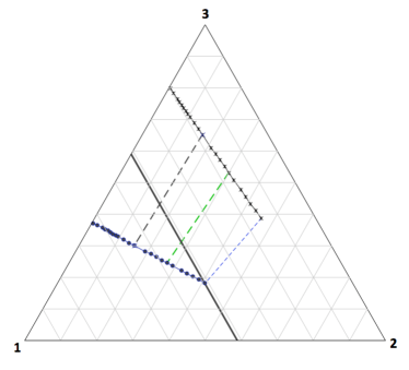
Figure 2: The thick black line indicates the path in overall composition tracked in the simulations. Symbols denote the compositions of the coexisting phases (crosses are for the gas; filled circles are liquid), observed along this path. Statistical uncertainties do not exceed the symbol sizes. A selection of representative tie lines are also shown (dashed lines). At $x_{2}^{0)}=0.409(1)$, the path leaves the region of phase coexistence.

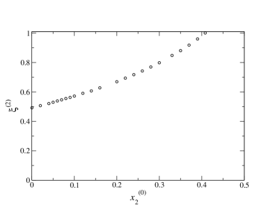
Figure 3: Measured value of the liquid phase fraction $\xi^{(2)}$ as a function of the path parameter $x_{2}^{(0)}$

VII Conclusions

In summary we have described a computational procedure for accurately and directly determining the phase behaviour that occurs along a path in the space of the overall composition of a ternary fluid mixture. For each state point along the path the method yields estimates for the concentrations of the coexisting phases whose tie line intersects that point, together with the phase fractions. Since finite-size corrections are exponentially small in the system size, the results are highly accurate even when the path of interest touches the coexistence boundary where the fraction of one phase vanishes. The simulation scheme, which is based on an extended sampling scheme in the semigrand canonical ensemble, uses histogram reweighting to track the path of interest. The only requirement is to bootstrap the method by determining the set of chemical potential differences that yield the overall concentrations corresponding to some point on the path. We have outlined how this can be achieved for pathway points corresponding to a single phase region of the phase diagram, or within a coexistence region in the limit in which one component vanishes, ie. for a binary system.

Our method is suitable for both fluid-fluid and fluid-solid phase coexistence, although in the latter case it needs to be combined with a sampling scheme such as phase switch Monte Carlo which allows the configuration spaces of the two phase to be connected by a trouble free sampling path Wilding and Bruce (2000); Wilding (2009). By virtue of the flexibility of histogram extrapolation, it is also readily generalizable to paths that involve simultaneous variation in composition and an external field (temperature or pressure). In future work we plan to demonstrate its utility for tracking such paths in the contexts of mixtures of four or more components for which compact phase diagrams do not exist.

References

- West (1982) D. West, Ternary Equilibrium Diagrams (Chapman and Hall, 1982).
- Tsang et al. (1995) P. C. Tsang, O. N. White, B. Y. Perigard, L. F. Vega, and A. Z. Panagiotopoulos, Fluid Phase Equilibria, 107, 31 (1995).
- Escobedo (1999) F. Escobedo, J. Chem. Phys., 110, 11999 (1999).
- Errington and Shen (2005) J. Errington and V. Shen, J. Chem. Phys., 123, 164103 (2005).
- Vrabec and Hasse (2002) J. Vrabec and H. Hasse, Mol. Phys., 100, 3375 (2002).
- Buzzacchi et al. (2006) M. Buzzacchi, P. Sollich, N. B. Wilding, and M. Müller, Phys. Rev. E, 73, 046110 (2006).
- Wilding et al. (2008) N. Wilding, P. Sollich, and M. Buzzacchi, Phys. Rev. E, 77, 011501 (2008).
- Kofke and Glandt (1988) D. A. Kofke and E. D. Glandt, Mol. Phys., 64, 1105 (1988).
- Frenkel and Smit (2002) D. Frenkel and B. Smit, Understanding Molecular Simulation (Academic, San Diego, 2002).
- Kofke and Glandt (1987) D. A. Kofke and E. D. Glandt, J. Chem. Phys., 87, 4881 (1987).
- Wilding (2003) N. B. Wilding, J. Chem. Phys., 119, 12163 (2003).
- Malasics et al. (2008) A. Malasics, D. Gillespie, and D. Boda, J. Chem. Phys., 128, 124102 (2008).
- Ferrenberg and Swendsen (1989) A. M. Ferrenberg and R. H. Swendsen, Phys. Rev. Lett., 63, 1195 (1989).
- Berg and Neuhaus (1992) B. A. Berg and T. Neuhaus, Phys. Rev. Lett., 68, 9 (1992).
- Note (1) Since in the SGCE the entire system fluctuates between phases, one utilizes the value of the order parameter associated with any given configuration in order to ascertain the corresponding phase label .
- Borgs and Kotecky (1992) C. Borgs and R. Kotecky, Phys. Rev. Lett., 68, 1734 (1992).
- Press et al. (2007) W. H. Press, S. A. Teukolsky, W. T. Vetterling, and B. P. Flannery, Numerical Recipes (Cambridge University Press, Cambridge, 2007).
- Wilding and Sollich (2002) N. B. Wilding and P. Sollich, J. Chem. Phys., 116, 7116 (2002).
- Wilding (1995) N. B. Wilding, Phys. Rev. E, 52, 602 (1995).
- Bruce and Wilding (2003) A. D. Bruce and N. B. Wilding, Adv. Chem. Phys, 127, 1 (2003).
- Wilding and Bruce (2000) N. B. Wilding and A. D. Bruce, Phys. Rev. Lett., 85, 5138 (2000).
- Wilding (2009) N. B. Wilding, J. Chem. Phys., 130, 104103 (2009).