1 Introduction
The approximation of singularly perturbed problems has retained the
attention of many authors in recent years. Let us mention [5 , 9 , 10 , 11 , 13 , 14 ] and the references quoted
there. However, in all references quoted no analysis is carried out for
differential operators with piecewise constant or piecewise smooth
coefficients. On the other hand, in many real life applications, the
differential operators have such piecewise coefficients that may have a very
large discrepancy. In that case, the solution of the problem will contain
boundary layers near the exterior boundary (as usual) but will also contain
interface layers along the interface where the coefficients have a large
jump. We refer to [4 ] for the description of this phenomenon in one
and two dimensions and to [12 ] for several numerical methods for the
robust approximation of such problems in one-dimension.
The goal of the present paper is to extend certain results from [12 ] to
two-dimensions. In particular, we consider a singularly perturbed
transmission problem in a domain with analytic boundary. Under the
assumption of the data also being analytic, we provide an asymptotic
expansion for the solution (in the style of [6 ] ) that provides
the necessary information for the design of a robust finite element method
that converges at an exponential rate as the degree p 𝑝 p [8 ] allow us to treat the outer and inner parts,
as well as the remainder (defined on one part of the domain). The results
obtained for the regularity of the interface layer (and the remainder
defined on the other part of the domain) are new and in line with those
reported in [12 ] for the one-dimensional analog of our model problem.
Our work closely follows what was done in [7 ] but also includes the
additional analysis for the interface layer.
The paper is organized as follows: In Section 2 3 4 5 6
Throughout the paper the spaces H s ( Ω ) superscript 𝐻 𝑠 Ω H^{s}(\Omega) s ≥ 0 𝑠 0 s\geq 0 Ω ⊂ ℝ 2 Ω superscript ℝ 2 \Omega\subset\mathbb{R}^{2} ∥ ⋅ ∥ s , Ω \|\cdot\|_{s,\Omega} | ⋅ | s , Ω |\cdot|_{s,\Omega} H 0 1 ( Ω ) superscript subscript 𝐻 0 1 Ω H_{0}^{1}(\Omega) H 0 1 ( Ω ) := { v ∈ H 1 ( Ω ) : v | ∂ Ω = 0 } assign superscript subscript 𝐻 0 1 Ω conditional-set 𝑣 superscript 𝐻 1 Ω evaluated-at 𝑣 Ω 0 H_{0}^{1}(\Omega):=\{v\in H^{1}(\Omega):\left.v\right|_{\partial\Omega}=0\} L p ( Ω ) superscript 𝐿 𝑝 Ω L^{p}(\Omega) p > 1 𝑝 1 p>1 ∥ ⋅ ∥ 0 , p , Ω \|\cdot\|_{0,p,\Omega} p 𝑝 p p = 2 𝑝 2 p=2 A ≲ B less-than-or-similar-to 𝐴 𝐵 A\lesssim B C 𝐶 C A 𝐴 A B 𝐵 B ε 𝜀 {\varepsilon} A ≤ C B 𝐴 𝐶 𝐵 A\leq CB
2 The model problem
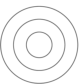
Let Ω + subscript Ω \Omega_{+} Ω − subscript Ω \Omega_{-} ℝ 2 superscript ℝ 2 \mathbb{R}^{2} ∂ Ω + subscript Ω \partial\Omega_{+} ∂ Ω − , subscript Ω \partial\Omega_{-}, ∂ Ω + ∩ ∂ Ω − = Σ subscript Ω subscript Ω Σ \partial\Omega_{+}\cap\partial\Omega_{-}=\Sigma ∂ Ω Ω \partial\Omega ∂ Ω ± subscript Ω plus-or-minus \partial\Omega_{\pm} Σ Σ \Sigma ∂ Ω + \ Σ \ subscript Ω Σ \partial\Omega_{+}\backslash\Sigma Σ Σ \Sigma Ω = Ω + ∪ Ω − Ω subscript Ω subscript Ω \Omega=\Omega_{+}\cup\Omega_{-} u 𝑢 u Ω Ω \Omega u + subscript 𝑢 u_{+} u − subscript 𝑢 u_{-} u 𝑢 u Ω + subscript Ω \Omega_{+} Ω − subscript Ω \Omega_{-} u ≡ ( u + , u − ) 𝑢 subscript 𝑢 subscript 𝑢 u\equiv\left(u_{+},u_{-}\right)
Figure 1: Example of the domains Ω + subscript Ω \Omega_{+} Ω − subscript Ω \Omega_{-}
We consider the following singularly perturbed transmission problem: Find u ε = ( u + ε , u − ε ) superscript 𝑢 𝜀 superscript subscript 𝑢 𝜀 superscript subscript 𝑢 𝜀 u^{\varepsilon}=\left(u_{+}^{\varepsilon},u_{-}^{\varepsilon}\right)
(1) − ε 2 Δ u + ε + u + ε superscript 𝜀 2 Δ superscript subscript 𝑢 𝜀 superscript subscript 𝑢 𝜀 \displaystyle-\varepsilon^{2}\Delta u_{+}^{\varepsilon}+u_{+}^{\varepsilon} = \displaystyle= f + in Ω + , subscript 𝑓 in subscript Ω \displaystyle f_{+}\text{ in }\Omega_{+},
(2) − Δ u − ε + u − ε Δ superscript subscript 𝑢 𝜀 superscript subscript 𝑢 𝜀 \displaystyle-\Delta u_{-}^{\varepsilon}+u_{-}^{\varepsilon} = \displaystyle= f − in Ω − , subscript 𝑓 in subscript Ω \displaystyle f_{-}\text{ in }\Omega_{-},
(3) u + ε superscript subscript 𝑢 𝜀 \displaystyle u_{+}^{\varepsilon} = \displaystyle= 0 on ∂ Ω + \ Σ , 0 on \ subscript Ω Σ \displaystyle 0\text{ on }\partial\Omega_{+}\backslash\Sigma,
(4) u − ε superscript subscript 𝑢 𝜀 \displaystyle u_{-}^{\varepsilon} = \displaystyle= 0 on ∂ Ω − \ Σ , 0 on \ subscript Ω Σ \displaystyle 0\text{ on }\partial\Omega_{-}\backslash\Sigma,
(5) u + ε − u − ε superscript subscript 𝑢 𝜀 superscript subscript 𝑢 𝜀 \displaystyle u_{+}^{\varepsilon}-u_{-}^{\varepsilon} = \displaystyle= 0 on Σ , 0 on Σ \displaystyle 0\text{ on }\Sigma,
(6) ε 2 ∂ u + ε ∂ ν − ∂ u − ε ∂ ν superscript 𝜀 2 superscript subscript 𝑢 𝜀 𝜈 superscript subscript 𝑢 𝜀 𝜈 \displaystyle\varepsilon^{2}\frac{\partial u_{+}^{\varepsilon}}{\partial\nu}-\frac{\partial u_{-}^{\varepsilon}}{\partial\nu} = \displaystyle= h on Σ , ℎ on Σ \displaystyle h\text{ on }\Sigma,
where Δ Δ \Delta ε ∈ ( 0 , 1 ] 𝜀 0 1 \varepsilon\in(0,1] f ± , h subscript 𝑓 plus-or-minus ℎ
f_{\pm},h ν 𝜈 \nu Σ Σ \Sigma Ω + subscript Ω \Omega_{+} 1 6 ε → 0 → 𝜀 0 \varepsilon\rightarrow 0
u + 0 superscript subscript 𝑢 0 \displaystyle u_{+}^{0} = \displaystyle= f + in Ω + , subscript 𝑓 in subscript Ω \displaystyle f_{+}\text{ in }\Omega_{+},
− Δ u − 0 + u − 0 Δ superscript subscript 𝑢 0 superscript subscript 𝑢 0 \displaystyle-\Delta u_{-}^{0}+u_{-}^{0} = \displaystyle= f − in Ω − , subscript 𝑓 in subscript Ω \displaystyle f_{-}\text{ in }\Omega_{-},
u + 0 superscript subscript 𝑢 0 \displaystyle u_{+}^{0} = \displaystyle= 0 on ∂ Ω + \ Σ , 0 on \ subscript Ω Σ \displaystyle 0\text{ on }\partial\Omega_{+}\backslash\Sigma,
u − 0 superscript subscript 𝑢 0 \displaystyle u_{-}^{0} = \displaystyle= 0 on ∂ Ω − \ Σ , 0 on \ subscript Ω Σ \displaystyle 0\text{ on }\partial\Omega_{-}\backslash\Sigma,
u + 0 − u − 0 superscript subscript 𝑢 0 superscript subscript 𝑢 0 \displaystyle u_{+}^{0}-u_{-}^{0} = \displaystyle= 0 on Σ , 0 on Σ \displaystyle 0\text{ on }\Sigma,
− ∂ u − 0 ∂ ν superscript subscript 𝑢 0 𝜈 \displaystyle-\frac{\partial u_{-}^{0}}{\partial\nu} = \displaystyle= h on Σ . ℎ on Σ \displaystyle h\text{ on }\Sigma.
Since, in general, f + subscript 𝑓 f_{+} f + = u + 0 subscript 𝑓 superscript subscript 𝑢 0 f_{+}=u_{+}^{0} ∂ Ω + \ Σ \ subscript Ω Σ \partial\Omega_{+}\backslash\Sigma f + = u − 0 subscript 𝑓 superscript subscript 𝑢 0 f_{+}=u_{-}^{0} Σ Σ \Sigma u ε superscript 𝑢 𝜀 u^{\varepsilon} ∂ Ω + \ Σ \ subscript Ω Σ \partial\Omega_{+}\backslash\Sigma Σ Σ \Sigma
We assume that the data of our problem is analytic and satisfies
(7) ‖ ∇ p f ± ‖ ∞ , Ω ± ≤ C f ± γ f ± p p ! ∀ p = 0 , 1 , 2 , … , formulae-sequence subscript norm superscript ∇ 𝑝 subscript 𝑓 plus-or-minus subscript Ω plus-or-minus
subscript 𝐶 subscript 𝑓 plus-or-minus superscript subscript 𝛾 subscript 𝑓 plus-or-minus 𝑝 𝑝 for-all 𝑝 0 1 2 …
\left\|\nabla^{p}f_{\pm}\right\|_{\infty,\Omega_{\pm}}\leq C_{f_{\pm}}\gamma_{f_{\pm}}^{p}p!\ \forall\ p=0,1,2,...,
(8) ‖ ∇ Σ p h ‖ ∞ , Σ ≤ C h γ h p p ! ∀ p = 0 , 1 , 2 , … , formulae-sequence subscript norm superscript subscript ∇ Σ 𝑝 ℎ Σ
subscript 𝐶 ℎ superscript subscript 𝛾 ℎ 𝑝 𝑝 for-all 𝑝 0 1 2 …
\left\|\nabla_{\Sigma}^{p}h\right\|_{\infty,\Sigma}\leq C_{h}\gamma_{h}^{p}p!\ \forall\ p=0,1,2,...,
for some positive constants C f ± , γ f ± , C h , γ h subscript 𝐶 subscript 𝑓 plus-or-minus subscript 𝛾 subscript 𝑓 plus-or-minus subscript 𝐶 ℎ subscript 𝛾 ℎ
C_{f_{\pm}},\gamma_{f_{\pm}},C_{h},\gamma_{h} ∇ Σ subscript ∇ Σ \nabla_{\Sigma} Σ Σ \Sigma 1 6 ε 𝜀 \varepsilon
Theorem 1
Let u ε = ( u + ε , u − ε ) superscript 𝑢 𝜀 superscript subscript 𝑢 𝜀 superscript subscript 𝑢 𝜀 u^{\varepsilon}=\left(u_{+}^{\varepsilon},u_{-}^{\varepsilon}\right) 1 6 7 8 C , K > 0 𝐶 𝐾
0 C,K>0
(9) ε ∥ D α u + ε ∥ 0 , Ω + + ∥ D α u − ε ∥ 0 , Ω − ≤ C ε K | α | max { | α | , ε − 1 } | α | ∀ α = 1 , 2 , … . \varepsilon\left\|D^{\alpha}u_{+}^{\varepsilon}\right\|_{0,\Omega_{+}}+\left\|D^{\alpha}u_{-}^{\varepsilon}\right\|_{0,\Omega_{-}}\leq C\varepsilon K^{\left|\alpha\right|}\max\left\{\left|\alpha\right|,\varepsilon^{-1}\right\}^{\left|\alpha\right|}\;\forall\;\alpha=1,2,....
Proof.
This follows from the local estimates
ε | u + ε | 2 , B x 0 ∩ Ω + + | u − ε | 2 , B x 0 ∩ Ω − ≤ C ( ε − 1 ∥ f + ∥ 0 , B x 0 ′ ∩ Ω + \displaystyle\varepsilon|u_{+}^{\varepsilon}|_{2,B_{x_{0}}\cap\Omega_{+}}+|u_{-}^{\varepsilon}|_{2,B_{x_{0}}\cap\Omega_{-}}\leq C(\varepsilon^{-1}\|f_{+}\|_{0,B^{\prime}_{x_{0}}\cap\Omega_{+}}
+ ∥ f − ∥ 0 , B x 0 ′ ∩ Ω − + ∥ h ∥ B x 0 ′ ∩ Σ + ε ∥ u + ε ∥ 1 , B x 0 ′ ∩ Ω + + ∥ u − ε ∥ 1 , B x 0 ′ ∩ Ω − ) , \displaystyle+\|f_{-}\|_{0,B^{\prime}_{x_{0}}\cap\Omega_{-}}+\|h\|_{B^{\prime}_{x_{0}}\cap\Sigma}+\varepsilon\|u_{+}^{\varepsilon}\|_{1,B^{\prime}_{x_{0}}\cap\Omega_{+}}+\|u_{-}^{\varepsilon}\|_{1,B^{\prime}_{x_{0}}\cap\Omega_{-}}),
for all sufficiently small balls B ¯ x 0 ⊂ B x 0 ′ subscript ¯ 𝐵 subscript 𝑥 0 subscript superscript 𝐵 ′ subscript 𝑥 0 \bar{B}_{x_{0}}\subset B^{\prime}_{x_{0}} x 0 ∈ Σ subscript 𝑥 0 Σ x_{0}\in\Sigma [7 ] or Theorems 5.2.2 and 5.3.8 in [3 ] ).
It should be noted that (9 u ε superscript 𝑢 𝜀 u^{\varepsilon} p 𝑝 p p > O ( ε − 1 ) 𝑝 𝑂 superscript 𝜀 1 p>O(\varepsilon^{-1}) p ≤ O ( ε − 1 ) 𝑝 𝑂 superscript 𝜀 1 p\leq O(\varepsilon^{-1})
3 Expansion of the solution
The solution of (1 6
(10) u ε = w ε + χ B L u B L ε + χ I L u I L ε + r ε , superscript 𝑢 𝜀 superscript 𝑤 𝜀 subscript 𝜒 𝐵 𝐿 superscript subscript 𝑢 𝐵 𝐿 𝜀 subscript 𝜒 𝐼 𝐿 superscript subscript 𝑢 𝐼 𝐿 𝜀 superscript 𝑟 𝜀 u^{\varepsilon}=w^{\varepsilon}+\chi_{BL}u_{BL}^{\varepsilon}+\chi_{IL}u_{IL}^{\varepsilon}+r^{\varepsilon},
where w ε superscript 𝑤 𝜀 w^{\varepsilon} u B L ε superscript subscript 𝑢 𝐵 𝐿 𝜀 u_{BL}^{\varepsilon} ∂ Ω + \ Σ \ subscript Ω Σ \partial\Omega_{+}\backslash\Sigma u I L ε superscript subscript 𝑢 𝐼 𝐿 𝜀 u_{IL}^{\varepsilon} Σ Σ \Sigma r ε superscript 𝑟 𝜀 r^{\varepsilon} χ B L subscript 𝜒 𝐵 𝐿 \chi_{BL} χ I L subscript 𝜒 𝐼 𝐿 \chi_{IL} 17 18 Ω Ω \Omega
In order to define the inner (boundary layer) expansion we introduce boundary fitted coordinates as follows: Let ( X ( θ ) , Y ( θ ) ) , θ ∈ [ 0 , L ] 𝑋 𝜃 𝑌 𝜃 𝜃
0 𝐿 \left(X(\theta),Y(\theta)\right),\theta\in[0,L] L − limit-from 𝐿 L- ∂ Ω + \ Σ \ subscript Ω Σ \partial\Omega_{+}\backslash\Sigma ( − Y ′ ( θ ) , X ′ ( θ ) ) superscript 𝑌 ′ 𝜃 superscript 𝑋 ′ 𝜃 \left(-Y^{\prime}(\theta),X^{\prime}(\theta)\right) Ω + subscript Ω \Omega_{+} κ + ( θ ) subscript 𝜅 𝜃 \kappa_{+}(\theta) ∂ Ω + \ Σ \ subscript Ω Σ \partial\Omega_{+}\backslash\Sigma 𝕋 L subscript 𝕋 𝐿 \mathbb{T}_{L} L 𝐿 L ∂ Ω Ω \partial\Omega X , Y 𝑋 𝑌
X,Y κ 𝜅 \kappa ρ 0 > 0 subscript 𝜌 0 0 \rho_{0}>0
(11) 0 < ρ 0 < 1 ‖ κ + ‖ L ∞ ( [ 0 , L ) ) . 0 subscript 𝜌 0 1 subscript norm subscript 𝜅 superscript 𝐿 0 𝐿 0<\rho_{0}<\frac{1}{\left\|\kappa_{+}\right\|_{L^{\infty}\left([0,L)\right)}}.
Then the mapping ψ : [ 0 , ρ 0 ] × 𝕋 L → Ω ¯ + : 𝜓 → 0 subscript 𝜌 0 subscript 𝕋 𝐿 subscript ¯ Ω \psi:[0,\rho_{0}]\times\mathbb{T}_{L}\rightarrow\overline{\Omega}_{+}
(12) ψ : ( ρ , θ ) → ( X ( θ ) − ρ Y ′ ( θ ) , Y ( θ ) + ρ X ′ ( θ ) ) : 𝜓 → 𝜌 𝜃 𝑋 𝜃 𝜌 superscript 𝑌 ′ 𝜃 𝑌 𝜃 𝜌 superscript 𝑋 ′ 𝜃 \psi:(\rho,\theta)\rightarrow\left(X(\theta)-\rho Y^{\prime}(\theta),Y(\theta)+\rho X^{\prime}(\theta)\right)
is real analytic on [ 0 , ρ 0 ] × 𝕋 L 0 subscript 𝜌 0 subscript 𝕋 𝐿 [0,\rho_{0}]\times\mathbb{T}_{L} ψ 𝜓 \psi ( 0 , ρ 0 ) × [ 0 , L ) 0 subscript 𝜌 0 0 𝐿 (0,\rho_{0})\times[0,L) Ω + 0 superscript subscript Ω 0 \Omega_{+}^{0} ∂ Ω + \ Σ \ subscript Ω Σ \partial\Omega_{+}\backslash\Sigma
(13) Ω + 0 = { z − ρ 𝐧 z : z ∈ ∂ Ω + \ Σ , 0 < ρ < ρ 0 } , superscript subscript Ω 0 conditional-set 𝑧 𝜌 subscript 𝐧 𝑧 formulae-sequence 𝑧 \ subscript Ω Σ 0 𝜌 subscript 𝜌 0 \Omega_{+}^{0}=\left\{z-\rho\mathbf{n}_{z}:z\in\partial\Omega_{+}\backslash\Sigma,0<\rho<\rho_{0}\right\},
with z = z ( θ ) = ( X ( θ ) , Y ( θ ) ) 𝑧 𝑧 𝜃 𝑋 𝜃 𝑌 𝜃 z=z(\theta)=\left(X(\theta),Y(\theta)\right) 𝐧 z subscript 𝐧 𝑧 \mathbf{n}_{z} z ∈ ∂ Ω + \ Σ 𝑧 \ subscript Ω Σ z\in\partial\Omega_{+}\backslash\Sigma
The interface layer will also be defined in a neighborhood of the interface Σ Σ \Sigma ( X Σ ( θ ) , Y Σ ( θ ) ) , θ ∈ [ 0 , L Σ ] subscript 𝑋 Σ 𝜃 subscript 𝑌 Σ 𝜃 𝜃
0 subscript 𝐿 Σ \left(X_{\Sigma}(\theta),Y_{\Sigma}(\theta)\right),\theta\in[0,L_{\Sigma}] L Σ − limit-from subscript 𝐿 Σ L_{\Sigma}- Σ Σ \Sigma κ Σ ( θ ) subscript 𝜅 Σ 𝜃 \kappa_{\Sigma}(\theta) Σ Σ \Sigma 𝕋 L Σ subscript 𝕋 subscript 𝐿 Σ \mathbb{T}_{L_{\Sigma}} L Σ subscript 𝐿 Σ L_{\Sigma} ρ Σ > 0 subscript 𝜌 Σ 0 \rho_{\Sigma}>0
(14) 0 < ρ Σ < 1 ‖ κ Σ ‖ L ∞ ( [ 0 , L Σ ) ) , 0 subscript 𝜌 Σ 1 subscript norm subscript 𝜅 Σ superscript 𝐿 0 subscript 𝐿 Σ 0<\rho_{\Sigma}<\frac{1}{\left\|\kappa_{\Sigma}\right\|_{L^{\infty}\left([0,L_{\Sigma})\right)}},
we define, analogously to (13
(15) Ω Σ 0 = { z − ρ 𝐧 Σ : z ∈ Σ , 0 < ρ < ρ Σ } , superscript subscript Ω Σ 0 conditional-set 𝑧 𝜌 subscript 𝐧 Σ formulae-sequence 𝑧 Σ 0 𝜌 subscript 𝜌 Σ \Omega_{\Sigma}^{0}=\left\{z-\rho\mathbf{n}_{\Sigma}:z\in\Sigma,0<\rho<\rho_{\Sigma}\right\},
with z = z ( θ ) = ( X Σ ( θ ) , Y Σ ( θ ) ) 𝑧 𝑧 𝜃 subscript 𝑋 Σ 𝜃 subscript 𝑌 Σ 𝜃 z=z(\theta)=\left(X_{\Sigma}(\theta),Y_{\Sigma}(\theta)\right) 𝐧 Σ subscript 𝐧 Σ \mathbf{n}_{\Sigma} z ∈ Σ 𝑧 Σ z\in\Sigma
The smooth cut-off functions χ B L , χ I L subscript 𝜒 𝐵 𝐿 subscript 𝜒 𝐼 𝐿
\chi_{BL},\chi_{IL} 10 ρ 1 , ρ 2 subscript 𝜌 1 subscript 𝜌 2
\rho_{1},\rho_{2}
(16) 0 < ρ 1 < ρ 0 , 0 < ρ 2 < ρ Σ formulae-sequence 0 subscript 𝜌 1 subscript 𝜌 0 0 subscript 𝜌 2 subscript 𝜌 Σ 0<\rho_{1}<\rho_{0}\;,\;0<\rho_{2}<\rho_{\Sigma}
and let χ B L , χ I L subscript 𝜒 𝐵 𝐿 subscript 𝜒 𝐼 𝐿
\chi_{BL},\chi_{IL} Ω ¯ + subscript ¯ Ω \overline{\Omega}_{+}
(17) χ B L ( x ) = { 1 for 0 ≤ dist ( x , ∂ Ω + \ Σ ) ≤ ρ 1 0 for dist ( x , ∂ Ω + \ Σ ) ≥ ( ρ 1 + ρ 0 ) / 2 , subscript 𝜒 𝐵 𝐿 𝑥 cases 1 for 0 dist 𝑥 \ subscript Ω Σ subscript 𝜌 1 0 for dist 𝑥 \ subscript Ω Σ subscript 𝜌 1 subscript 𝜌 0 2 \chi_{BL}(x)=\left\{\begin{array}[]{cc}1&\text{for }0\leq\text{dist}(x,\partial\Omega_{+}\backslash\Sigma)\leq\rho_{1}\text{ \ \ \ \ \ \ \ }\\
0&\text{for dist}(x,\partial\Omega_{+}\backslash\Sigma)\geq(\rho_{1}+\rho_{0})/2\end{array}\right.,
(18) χ I L ( x ) = { 1 for 0 ≤ dist ( x , Σ ) ≤ ρ 2 0 for dist ( x , Σ ) ≥ ( ρ 2 + ρ Σ ) / 2 . subscript 𝜒 𝐼 𝐿 𝑥 cases 1 for 0 dist 𝑥 Σ subscript 𝜌 2 0 for dist 𝑥 Σ subscript 𝜌 2 subscript 𝜌 Σ 2 \chi_{IL}(x)=\left\{\begin{array}[]{cc}1&\text{for }0\leq\text{dist}(x,\Sigma)\text{ }\leq\rho_{2}\text{\ \ \ \ \ \ \ }\\
0&\text{for dist}(x,\Sigma)\geq(\rho_{2}+\rho_{\Sigma})/2\end{array}\right..
The above will be utilized in sections 3.2 3.3
3.1 Construction and regularity of the outer part
We begin by constructing the outer part w ε superscript 𝑤 𝜀 w^{\varepsilon} 10 u ε = ( u + ε , u − ε ) superscript 𝑢 𝜀 superscript subscript 𝑢 𝜀 superscript subscript 𝑢 𝜀 u^{\varepsilon}=\left(u_{+}^{\varepsilon},u_{-}^{\varepsilon}\right) ε 𝜀 \varepsilon
(19) u ± ε = u 0 ± + ε u 1 ± + ε 2 u 2 ± + … superscript subscript 𝑢 plus-or-minus 𝜀 superscript subscript 𝑢 0 plus-or-minus 𝜀 superscript subscript 𝑢 1 plus-or-minus superscript 𝜀 2 superscript subscript 𝑢 2 plus-or-minus … u_{\pm}^{\varepsilon}\;=u_{0}^{\pm}+\varepsilon u_{1}^{\pm}+\varepsilon^{2}u_{2}^{\pm}+...
and insert it in the differential equations (1 6 ε 𝜀 \varepsilon u j ± , j = 0 , 1 , 2 , … formulae-sequence superscript subscript 𝑢 𝑗 plus-or-minus 𝑗
0 1 2 …
u_{j}^{\pm},j=0,1,2,... u j + superscript subscript 𝑢 𝑗 u_{j}^{+}
(20) u 0 + = f + , u 2 j + = Δ ( 2 j + 2 ) f + , u 2 j − 1 + = 0 , j = 1 , 2 , … formulae-sequence superscript subscript 𝑢 0 subscript 𝑓 formulae-sequence superscript subscript 𝑢 2 𝑗 superscript Δ 2 𝑗 2 subscript 𝑓 formulae-sequence superscript subscript 𝑢 2 𝑗 1 0 𝑗 1 2 …
u_{0}^{+}=f_{+},\;u_{2j}^{+}=\Delta^{(2j+2)}f_{+},\;u_{2j-1}^{+}=0,\;j=1,2,...
where Δ ( i ) superscript Δ 𝑖 \Delta^{(i)} u 0 − superscript subscript 𝑢 0 u_{0}^{-}
(21) − Δ u 0 − + u 0 − Δ superscript subscript 𝑢 0 superscript subscript 𝑢 0 \displaystyle-\Delta u_{0}^{-}+u_{0}^{-} = \displaystyle= f − in Ω − , subscript 𝑓 in subscript Ω \displaystyle f_{-}\text{ in }\Omega_{-},
(22) u 0 − superscript subscript 𝑢 0 \displaystyle u_{0}^{-} = \displaystyle= 0 on ∂ Ω − \ Σ , 0 on \ subscript Ω Σ \displaystyle 0\text{ on }\partial\Omega_{-}\backslash\Sigma,
(23) ∂ u 0 − ∂ ν superscript subscript 𝑢 0 𝜈 \displaystyle\frac{\partial u_{0}^{-}}{\partial\nu} = \displaystyle= − h on Σ . ℎ on Σ \displaystyle-h\text{ on }\Sigma.
For j ≥ 1 𝑗 1 j\geq 1 u 2 j − 1 − = 0 superscript subscript 𝑢 2 𝑗 1 0 u_{2j-1}^{-}=0
(24) − Δ u 2 j − + u 2 j − Δ superscript subscript 𝑢 2 𝑗 superscript subscript 𝑢 2 𝑗 \displaystyle-\Delta u_{2j}^{-}+u_{2j}^{-} = \displaystyle= 0 in Ω − , 0 in subscript Ω \displaystyle 0\text{ in }\Omega_{-},
(25) u 2 j − superscript subscript 𝑢 2 𝑗 \displaystyle u_{2j}^{-} = \displaystyle= 0 on ∂ Ω − \ Σ , 0 on \ subscript Ω Σ \displaystyle 0\text{ on }\partial\Omega_{-}\backslash\Sigma,
(26) ∂ u 2 j − ∂ ν superscript subscript 𝑢 2 𝑗 𝜈 \displaystyle\frac{\partial u_{2j}^{-}}{\partial\nu} = \displaystyle= ∂ u 2 j − 2 + ∂ ν on Σ . superscript subscript 𝑢 2 𝑗 2 𝜈 on Σ \displaystyle\frac{\partial u_{2j-2}^{+}}{\partial\nu}\text{ on }\Sigma.
Note that u 2 j − superscript subscript 𝑢 2 𝑗 u_{2j}^{-} Ω − subscript Ω \Omega_{-} u 2 j − superscript subscript 𝑢 2 𝑗 u_{2j}^{-} 34
Using the above, we can define the outer expansion as
(27) w ± ≡ w M ± = ∑ j = 0 𝑀 ε 2 j u 2 j ± , superscript 𝑤 plus-or-minus superscript subscript 𝑤 𝑀 plus-or-minus 𝑀 𝑗 0 superscript 𝜀 2 𝑗 superscript subscript 𝑢 2 𝑗 plus-or-minus w^{\pm}\equiv w_{M}^{\pm}=\overset{M}{\underset{j=0}{\mathop{\displaystyle\sum}}}\varepsilon^{2j}u_{2j}^{\pm},
where M 𝑀 M 1 / ε 1 𝜀 1/\varepsilon [5 ] , [7 ] ). It is not difficult to see
that
(28) ( − ε 2 Δ w M + + w M + ) − f + = ε 2 M + 2 Δ ( M + 1 ) f + superscript 𝜀 2 Δ superscript subscript 𝑤 𝑀 superscript subscript 𝑤 𝑀 subscript 𝑓 superscript 𝜀 2 𝑀 2 superscript Δ 𝑀 1 subscript 𝑓 \left(-\varepsilon^{2}\Delta w_{M}^{+}+w_{M}^{+}\right)-f_{+}=\varepsilon^{2M+2}\Delta^{(M+1)}f_{+}
and
(29) ( − Δ w M − + w M − ) − f − = 0 . Δ superscript subscript 𝑤 𝑀 superscript subscript 𝑤 𝑀 subscript 𝑓 0 \left(-\Delta w_{M}^{-}+w_{M}^{-}\right)-f_{-}=0.
Moreover, we have the following theorem.
Theorem 2
Let w M ± superscript subscript 𝑤 𝑀 plus-or-minus w_{M}^{\pm} 27 K 1 subscript 𝐾 1 K_{1} C 𝐶 C ε M 𝜀 𝑀 \varepsilon M
(30) ‖ D α w M + ‖ ∞ , Ω + ≲ K 1 | α | | α | ! ∀ α ∈ ℕ 0 2 , less-than-or-similar-to subscript norm superscript 𝐷 𝛼 superscript subscript 𝑤 𝑀 subscript Ω
superscript subscript 𝐾 1 𝛼 𝛼 for-all 𝛼 superscript subscript ℕ 0 2 \left\|D^{\alpha}w_{M}^{+}\right\|_{\infty,\Omega_{+}}\lesssim K_{1}^{|\alpha|}|\alpha|!\;\forall\;\alpha\in\mathbb{N}_{0}^{2},
(31) ‖ w M − ‖ k , Ω − ≲ C k + 1 k ! . less-than-or-similar-to subscript norm superscript subscript 𝑤 𝑀 𝑘 subscript Ω
superscript 𝐶 𝑘 1 𝑘 \left\|w_{M}^{-}\right\|_{k,\Omega_{-}}\lesssim C^{k+1}k!\;.
Proof. From Theorem 2.2 of [8 ] we have that
‖ D α w M + ‖ ∞ , Ω + ≲ K 1 | α | | α | ! ( 1 + ( 2 M ε K 2 ) 2 M ) ∀ α ∈ ℕ 0 2 , less-than-or-similar-to subscript norm superscript 𝐷 𝛼 superscript subscript 𝑤 𝑀 subscript Ω
superscript subscript 𝐾 1 𝛼 𝛼 1 superscript 2 𝑀 𝜀 subscript 𝐾 2 2 𝑀 for-all 𝛼 superscript subscript ℕ 0 2 \left\|D^{\alpha}w_{M}^{+}\right\|_{\infty,\Omega_{+}}\lesssim K_{1}^{|\alpha|}|\alpha|!\left(1+\left(2M\varepsilon K_{2}\right)^{2M}\right)\;\forall\;\alpha\in\mathbb{N}_{0}^{2},
so if 2 M ε K 2 < 1 2 𝑀 𝜀 subscript 𝐾 2 1 2M\varepsilon K_{2}<1 30 31 u 0 − superscript subscript 𝑢 0 u_{0}^{-} 21 23 u 0 − superscript subscript 𝑢 0 u_{0}^{-} [3 ] ,
and moreover
| u 0 − | k , Ω − ≤ C k + 1 k ! ∀ k ∈ ℕ 0 . subscript superscript subscript 𝑢 0 𝑘 subscript Ω
superscript 𝐶 𝑘 1 𝑘 for-all 𝑘 subscript ℕ 0 \left|u_{0}^{-}\right|_{k,\Omega_{-}}\leq C^{k+1}k!\;\forall\;k\in\mathbb{N}_{0}.
Next, we consider u 2 j − , superscript subscript 𝑢 2 𝑗 u_{2j}^{-}, j = 0 , 1 , … , 𝑗 0 1 …
j=0,1,..., 24 26 24 26
‖ u 2 j − ‖ 1 , Ω − 2 = ∫ Σ ∂ u 2 j − 2 + ∂ ν u 2 j − ≲ ‖ ∂ u 2 j − 2 + ∂ ν ‖ 0 , Σ ‖ u 2 j − ‖ 1 , Ω − , superscript subscript norm superscript subscript 𝑢 2 𝑗 1 subscript Ω
2 Σ superscript subscript 𝑢 2 𝑗 2 𝜈 superscript subscript 𝑢 2 𝑗 less-than-or-similar-to subscript norm superscript subscript 𝑢 2 𝑗 2 𝜈 0 Σ
subscript norm superscript subscript 𝑢 2 𝑗 1 subscript Ω
\left\|u_{2j}^{-}\right\|_{1,\Omega_{-}}^{2}=\underset{\Sigma}{\mathop{\displaystyle\int}}\frac{\partial u_{2j-2}^{+}}{\partial\nu}u_{2j}^{-}\lesssim\left\|\frac{\partial u_{2j-2}^{+}}{\partial\nu}\right\|_{0,\Sigma}\left\|u_{2j}^{-}\right\|_{1,\Omega_{-}},
which, using (20
(32) ‖ u 2 j − ‖ 1 , Ω − ≲ ‖ ∂ u 2 j − 2 + ∂ ν ‖ 0 , Σ ≲ ‖ ∂ ( Δ 2 j f + ) ∂ ν ‖ 0 , Σ ≲ ‖ ∇ 4 j + 1 f + ‖ ∞ , Ω + . less-than-or-similar-to subscript norm superscript subscript 𝑢 2 𝑗 1 subscript Ω
subscript norm superscript subscript 𝑢 2 𝑗 2 𝜈 0 Σ
less-than-or-similar-to subscript norm superscript Δ 2 𝑗 subscript 𝑓 𝜈 0 Σ
less-than-or-similar-to subscript norm superscript ∇ 4 𝑗 1 subscript 𝑓 subscript Ω
\left\|u_{2j}^{-}\right\|_{1,\Omega_{-}}\lesssim\left\|\frac{\partial u_{2j-2}^{+}}{\partial\nu}\right\|_{0,\Sigma}\lesssim\left\|\frac{\partial\left(\Delta^{2j}f_{+}\right)}{\partial\nu}\right\|_{0,\Sigma}\lesssim\left\|\nabla^{4j+1}f_{+}\right\|_{\infty,\Omega_{+}}.
From [3 ] we have that there exists C ∈ ℝ + 𝐶 superscript ℝ C\in\mathbb{R}^{+}
(33) 1 k ! | u 2 j − | k , Ω − ≤ C k + 1 { ∑ ℓ = 1 𝑘 1 ℓ ! ‖ ∂ u 2 j − ∂ ν ∥ ℓ + 1 2 , Σ + ‖ u 2 j − ‖ 1 , Ω − } , 1 𝑘 subscript superscript subscript 𝑢 2 𝑗 𝑘 subscript Ω
superscript 𝐶 𝑘 1 conditional-set ℓ 1 𝑘 1 ℓ evaluated-at superscript subscript 𝑢 2 𝑗 𝜈 ℓ 1 2 Σ
subscript norm superscript subscript 𝑢 2 𝑗 1 subscript Ω
\frac{1}{k!}\left|u_{2j}^{-}\right|_{k,\Omega_{-}}\leq C^{k+1}\left\{\underset{\ell=1}{\overset{k}{\mathop{\displaystyle\sum}}}\frac{1}{\ell!}\left\|\frac{\partial u_{2j}^{-}}{\partial\nu}\right\|_{\ell+\frac{1}{2},\Sigma}+\left\|u_{2j}^{-}\right\|_{1,\Omega_{-}}\right\},
and we note that (see eq. (26
‖ ∂ u 2 j − ∂ ν ‖ ℓ + 1 2 , Σ 2 superscript subscript norm superscript subscript 𝑢 2 𝑗 𝜈 ℓ 1 2 Σ
2 \displaystyle\left\|\frac{\partial u_{2j}^{-}}{\partial\nu}\right\|_{\ell+\frac{1}{2},\Sigma}^{2} = \displaystyle= ‖ ∂ u 2 j − 2 + ∂ ν ‖ ℓ + 1 2 , Σ 2 = ‖ ∂ ( Δ 2 j f + ) ∂ ν ‖ ℓ + 1 2 , Σ 2 ≲ ‖ Δ 2 j f + ‖ ℓ + 1 , Ω + 2 superscript subscript norm superscript subscript 𝑢 2 𝑗 2 𝜈 ℓ 1 2 Σ
2 superscript subscript norm superscript Δ 2 𝑗 subscript 𝑓 𝜈 ℓ 1 2 Σ
2 less-than-or-similar-to superscript subscript norm superscript Δ 2 𝑗 subscript 𝑓 ℓ 1 subscript Ω
2 \displaystyle\left\|\frac{\partial u_{2j-2}^{+}}{\partial\nu}\right\|_{\ell+\frac{1}{2},\Sigma}^{2}=\left\|\frac{\partial\left(\Delta^{2j}f_{+}\right)}{\partial\nu}\right\|_{\ell+\frac{1}{2},\Sigma}^{2}\lesssim\left\|\Delta^{2j}f_{+}\right\|_{\ell+1,\Omega_{+}}^{2}
≲ less-than-or-similar-to \displaystyle\lesssim ∑ | α | ≤ ℓ + 1 ∫ Ω + | D α Δ 2 j f + | 2 d x ≲ ∑ | α | ≤ ℓ + 1 ‖ D α Δ 2 j f + ‖ ∞ , Ω + 2 . less-than-or-similar-to 𝛼 ℓ 1 subscript Ω superscript superscript 𝐷 𝛼 superscript Δ 2 𝑗 subscript 𝑓 2 𝑑 𝑥 𝛼 ℓ 1 superscript subscript norm superscript 𝐷 𝛼 superscript Δ 2 𝑗 subscript 𝑓 subscript Ω
2 \displaystyle\underset{\left|\alpha\right|\leq\ell+1}{\mathop{\displaystyle\sum}}\ \underset{\Omega_{+}}{\mathop{\displaystyle\int}}\left|D^{\alpha}\Delta^{2j}f_{+}\right|^{2}dx\lesssim\underset{\left|\alpha\right|\leq\ell+1}{\mathop{\displaystyle\sum}}\left\|D^{\alpha}\Delta^{2j}f_{+}\right\|_{\infty,\Omega_{+}}^{2}.
Hence, (33 7 32
1 k ! | u 2 j − | k , Ω − 1 𝑘 subscript superscript subscript 𝑢 2 𝑗 𝑘 subscript Ω
\displaystyle\frac{1}{k!}\left|u_{2j}^{-}\right|_{k,\Omega_{-}} ≤ \displaystyle\leq C k + 1 { ∑ ℓ = 1 𝑘 1 ℓ ! ∑ | α | ≤ ℓ + 1 ‖ D α Δ 2 j f + ∥ ∞ , Ω + + ‖ Δ 2 j f + ‖ ∞ , Σ } superscript 𝐶 𝑘 1 conditional-set ℓ 1 𝑘 1 ℓ 𝛼 ℓ 1 evaluated-at superscript 𝐷 𝛼 superscript Δ 2 𝑗 subscript 𝑓 subscript Ω
subscript norm superscript Δ 2 𝑗 subscript 𝑓 Σ
\displaystyle C^{k+1}\left\{\underset{\ell=1}{\overset{k}{\mathop{\displaystyle\sum}}}\frac{1}{\ell!}\underset{\left|\alpha\right|\leq\ell+1}{\mathop{\displaystyle\sum}}\left\|D^{\alpha}\Delta^{2j}f_{+}\right\|_{\infty,\Omega_{+}}+\left\|\Delta^{2j}f_{+}\right\|_{\infty,\Sigma}\right\}
≲ less-than-or-similar-to \displaystyle\lesssim C k + 1 { ∑ ℓ = 1 𝑘 1 ℓ ! ∑ | α | ≤ ℓ + 1 γ | α | + 2 j ( | α | + 2 j ) ! + γ 2 j ( 2 j ) ! } superscript 𝐶 𝑘 1 ℓ 1 𝑘 1 ℓ 𝛼 ℓ 1 superscript 𝛾 𝛼 2 𝑗 𝛼 2 𝑗 superscript 𝛾 2 𝑗 2 𝑗 \displaystyle C^{k+1}\left\{\underset{\ell=1}{\overset{k}{\mathop{\displaystyle\sum}}}\frac{1}{\ell!}\underset{\left|\alpha\right|\leq\ell+1}{\mathop{\displaystyle\sum}}\gamma^{\left|\alpha\right|+2j}\left(\left|\alpha\right|+2j\right)!+\gamma^{2j}\left(2j\right)!\right\}
≲ less-than-or-similar-to \displaystyle\lesssim C k + 1 ∑ ℓ = 1 𝑘 ℓ 2 γ ℓ + 2 j ( ℓ + 2 j ) ! superscript 𝐶 𝑘 1 ℓ 1 𝑘 superscript ℓ 2 superscript 𝛾 ℓ 2 𝑗 ℓ 2 𝑗 \displaystyle C^{k+1}\underset{\ell=1}{\overset{k}{\mathop{\displaystyle\sum}}}\ell^{2}\gamma^{\ell+2j}\left(\ell+2j\right)!
≲ less-than-or-similar-to \displaystyle\lesssim C k + 1 k 2 ( 2 j ) ! ∑ ℓ = 1 𝑘 γ k + 2 j ( ℓ + 2 j ℓ ) superscript 𝐶 𝑘 1 superscript 𝑘 2 2 𝑗 ℓ 1 𝑘 superscript 𝛾 𝑘 2 𝑗 binomial ℓ 2 𝑗 ℓ \displaystyle C^{k+1}k^{2}\left(2j\right)!\underset{\ell=1}{\overset{k}{\mathop{\displaystyle\sum}}}\gamma^{k+2j}\binom{\ell+2j}{\ell}
≲ less-than-or-similar-to \displaystyle\lesssim C 1 k + 1 ( 2 j ) ! ( 1 + γ ) k + 2 j γ 2 j superscript subscript 𝐶 1 𝑘 1 2 𝑗 superscript 1 𝛾 𝑘 2 𝑗 superscript 𝛾 2 𝑗 \displaystyle C_{1}^{k+1}\left(2j\right)!\left(1+\gamma\right)^{k+2j}\gamma^{2j}
≲ less-than-or-similar-to \displaystyle\lesssim C 1 k + 1 ( 2 j ) ! γ 1 2 j superscript subscript 𝐶 1 𝑘 1 2 𝑗 superscript subscript 𝛾 1 2 𝑗 \displaystyle C_{1}^{k+1}\left(2j\right)!\gamma_{1}^{2j}
for a suitable C 1 , γ 1 > 0 . subscript 𝐶 1 subscript 𝛾 1
0 C_{1},\gamma_{1}>0. u 2 j − superscript subscript 𝑢 2 𝑗 u_{2j}^{-} ∀ j = 0 , 1 , … for-all 𝑗 0 1 …
\forall\;j=0,1,...
(34) | u 2 j − | k , Ω − ≲ C 1 k + 1 k ! ( 2 j ) ! γ 1 2 j , k ∈ ℕ . formulae-sequence less-than-or-similar-to subscript superscript subscript 𝑢 2 𝑗 𝑘 subscript Ω
superscript subscript 𝐶 1 𝑘 1 𝑘 2 𝑗 superscript subscript 𝛾 1 2 𝑗 𝑘 ℕ \left|u_{2j}^{-}\right|_{k,\Omega_{-}}\lesssim C_{1}^{k+1}k!\left(2j\right)!\gamma_{1}^{2j}\;,\;k\in\mathbb{N}.
Thus, from the definition of w M − superscript subscript 𝑤 𝑀 w_{M}^{-}
| w M − | k , Ω − subscript superscript subscript 𝑤 𝑀 𝑘 subscript Ω
\displaystyle\left|w_{M}^{-}\right|_{k,\Omega_{-}} ≤ \displaystyle\leq ∑ j = 0 𝑀 ε 2 j | u 2 j − | k , Ω − ≲ C 1 k + 1 k ! ∑ j = 0 𝑀 ε 2 j ( 2 j ) ! γ 1 2 j less-than-or-similar-to 𝑗 0 𝑀 superscript 𝜀 2 𝑗 subscript superscript subscript 𝑢 2 𝑗 𝑘 subscript Ω
superscript subscript 𝐶 1 𝑘 1 𝑘 𝑗 0 𝑀 superscript 𝜀 2 𝑗 2 𝑗 superscript subscript 𝛾 1 2 𝑗 \displaystyle\underset{j=0}{\overset{M}{\mathop{\displaystyle\sum}}}\varepsilon^{2j}\left|u_{2j}^{-}\right|_{k,\Omega_{-}}\lesssim C_{1}^{k+1}k!\underset{j=0}{\overset{M}{\mathop{\displaystyle\sum}}}\varepsilon^{2j}\left(2j\right)!\gamma_{1}^{2j}
≲ less-than-or-similar-to \displaystyle\lesssim C 1 k + 1 k ! ∑ j = 0 𝑀 ε 2 j ( 2 M ) 2 j γ 1 2 j ≲ C 1 k + 1 k ! ∑ j = 0 𝑀 ( 2 ε M γ 1 ) 2 j less-than-or-similar-to superscript subscript 𝐶 1 𝑘 1 𝑘 𝑗 0 𝑀 superscript 𝜀 2 𝑗 superscript 2 𝑀 2 𝑗 superscript subscript 𝛾 1 2 𝑗 superscript subscript 𝐶 1 𝑘 1 𝑘 𝑗 0 𝑀 superscript 2 𝜀 𝑀 subscript 𝛾 1 2 𝑗 \displaystyle C_{1}^{k+1}k!\underset{j=0}{\overset{M}{\mathop{\displaystyle\sum}}}\varepsilon^{2j}\left(2M\right)^{2j}\gamma_{1}^{2j}\lesssim C_{1}^{k+1}k!\underset{j=0}{\overset{M}{\mathop{\displaystyle\sum}}}\left(2\varepsilon M\gamma_{1}\right)^{2j}
≲ less-than-or-similar-to \displaystyle\lesssim C k + 1 k ! , superscript 𝐶 𝑘 1 𝑘 \displaystyle C^{k+1}k!,
provided 2 ε M γ 1 < 1 2 𝜀 𝑀 subscript 𝛾 1 1 2\varepsilon M\gamma_{1}<1\,\ 31
3.2 Construction and regularity of the boundary layers along ∂ Ω + \ Σ \ subscript Ω Σ \partial\Omega_{+}\backslash\Sigma
Boundary layers are introduced in order to account for the fact that the
function w M + superscript subscript 𝑤 𝑀 w_{M}^{+} ∂ Ω + \ Σ \ subscript Ω Σ \partial\Omega_{+}\backslash\Sigma 28 [8 ] , so we will only outline the
procedure and quote the relevant results from [8 ] . The boundary layer
correction u B L ε superscript subscript 𝑢 𝐵 𝐿 𝜀 u_{BL}^{\varepsilon} w M + superscript subscript 𝑤 𝑀 w_{M}^{+}
(35) L ε u B L ε subscript 𝐿 𝜀 superscript subscript 𝑢 𝐵 𝐿 𝜀 \displaystyle L_{\varepsilon}u_{BL}^{\varepsilon} = \displaystyle= 0 in Ω + , 0 in subscript Ω \displaystyle 0\text{ in }\Omega_{+},
(36) u B L ε superscript subscript 𝑢 𝐵 𝐿 𝜀 \displaystyle u_{BL}^{\varepsilon} = \displaystyle= − w M + on ∂ Ω + \ Σ , superscript subscript 𝑤 𝑀 on \ subscript Ω Σ \displaystyle-w_{M}^{+}\text{ on }\partial\Omega_{+}\backslash\Sigma,
where L ε subscript 𝐿 𝜀 L_{\varepsilon}
(37) L ε u := − ε 2 Δ u + u . assign subscript 𝐿 𝜀 𝑢 superscript 𝜀 2 Δ 𝑢 𝑢 L_{\varepsilon}u:=-\varepsilon^{2}\Delta u+u.
With κ + ( θ ) subscript 𝜅 𝜃 \kappa_{+}(\theta) ∂ Ω + \ Σ \ subscript Ω Σ \partial\Omega_{+}\backslash\Sigma
σ + ( ρ , θ ) = 1 1 − κ + ( θ ) ρ , subscript 𝜎 𝜌 𝜃 1 1 subscript 𝜅 𝜃 𝜌 \sigma_{+}(\rho,\theta)=\frac{1}{1-\kappa_{+}(\theta)\rho},
and we have (see, e.g. [1 ] )
Δ u ( ρ , θ ) = ∂ ρ 2 u − κ + ( θ ) σ + ( ρ , θ ) ∂ ρ u + σ + 2 ( ρ , θ ) ∂ θ 2 u + ρ κ + ′ ( θ ) σ + 3 ( ρ , θ ) ∂ θ u . Δ 𝑢 𝜌 𝜃 superscript subscript 𝜌 2 𝑢 subscript 𝜅 𝜃 subscript 𝜎 𝜌 𝜃 subscript 𝜌 𝑢 superscript subscript 𝜎 2 𝜌 𝜃 superscript subscript 𝜃 2 𝑢 𝜌 superscript subscript 𝜅 ′ 𝜃 superscript subscript 𝜎 3 𝜌 𝜃 subscript 𝜃 𝑢 \Delta u(\rho,\theta)=\partial_{\rho}^{2}u-\kappa_{+}(\theta)\sigma_{+}(\rho,\theta)\partial_{\rho}u+\sigma_{+}^{2}(\rho,\theta)\partial_{\theta}^{2}u+\rho\kappa_{+}^{\prime}(\theta)\sigma_{+}^{3}(\rho,\theta)\partial_{\theta}u.
Introducing the stretched variable ρ ^ = ρ / ε ^ 𝜌 𝜌 𝜀 \widehat{\rho}=\rho/\varepsilon L ε subscript 𝐿 𝜀 L_{\varepsilon}
(38) L ε = − ∂ ρ ^ 2 + Id + ε κ + ( θ ) σ + ( ε ρ ^ , θ ) ∂ ρ ^ − ε 2 σ + 2 ( ε ρ ^ , θ ) − ε 3 ρ ^ κ + ′ ( θ ) σ + 3 ( ε ρ ^ , θ ) ∂ θ . subscript 𝐿 𝜀 superscript subscript ^ 𝜌 2 Id 𝜀 subscript 𝜅 𝜃 subscript 𝜎 𝜀 ^ 𝜌 𝜃 subscript ^ 𝜌 superscript 𝜀 2 superscript subscript 𝜎 2 𝜀 ^ 𝜌 𝜃 superscript 𝜀 3 ^ 𝜌 superscript subscript 𝜅 ′ 𝜃 superscript subscript 𝜎 3 𝜀 ^ 𝜌 𝜃 subscript 𝜃 L_{\varepsilon}=-\partial_{\widehat{\rho}}^{2}+\text{Id}+\varepsilon\kappa_{+}(\theta)\sigma_{+}(\varepsilon\widehat{\rho},\theta)\partial_{\widehat{\rho}}-\varepsilon^{2}\sigma_{+}^{2}(\varepsilon\widehat{\rho},\theta)-\varepsilon^{3}\widehat{\rho}\kappa_{+}^{\prime}(\theta)\sigma_{+}^{3}(\varepsilon\widehat{\rho},\theta)\partial_{\theta}.
Expanding the above in power series of ε 𝜀 \varepsilon
(39) L ε = ∑ i = 0 ∞ ε i L i , subscript 𝐿 𝜀 𝑖 0 infinity superscript 𝜀 𝑖 subscript 𝐿 𝑖 L_{\varepsilon}=\underset{i=0}{\overset{\infty}{\mathop{\displaystyle\sum}}}\varepsilon^{i}L_{i},
where the operators L i subscript 𝐿 𝑖 L_{i} [8 ] )
(40) L 0 = − ∂ ρ ^ 2 + Id , L i = − ρ ^ i − 1 a 1 i − 1 ∂ ρ ^ − ρ ^ i − 2 a 2 i − 2 ∂ θ 2 − ρ ^ i − 2 a 3 i − 3 ∂ θ , i ≥ 1 , formulae-sequence subscript 𝐿 0 superscript subscript ^ 𝜌 2 Id formulae-sequence subscript 𝐿 𝑖 superscript ^ 𝜌 𝑖 1 superscript subscript 𝑎 1 𝑖 1 subscript ^ 𝜌 superscript ^ 𝜌 𝑖 2 superscript subscript 𝑎 2 𝑖 2 superscript subscript 𝜃 2 superscript ^ 𝜌 𝑖 2 superscript subscript 𝑎 3 𝑖 3 subscript 𝜃 𝑖 1 L_{0}=-\partial_{\widehat{\rho}}^{2}+\text{Id},\;L_{i}=-\widehat{\rho}^{i-1}a_{1}^{i-1}\partial_{\widehat{\rho}}-\widehat{\rho}^{i-2}a_{2}^{i-2}\partial_{\theta}^{2}-\widehat{\rho}^{i-2}a_{3}^{i-3}\partial_{\theta},\;i\geq 1,
and the coefficients a j i superscript subscript 𝑎 𝑗 𝑖 a_{j}^{i}
(41) a 1 i = − [ κ + ( θ ) ] i + 1 , a 2 i = ( i + 1 ) [ κ + ( θ ) ] i , a 3 i = ( i + 1 ) ( i + 2 ) 2 [ κ + ( θ ) ] i κ + ′ ( θ ) , i ∈ ℕ 0 , formulae-sequence superscript subscript 𝑎 1 𝑖 superscript delimited-[] subscript 𝜅 𝜃 𝑖 1 formulae-sequence superscript subscript 𝑎 2 𝑖 𝑖 1 superscript delimited-[] subscript 𝜅 𝜃 𝑖 formulae-sequence superscript subscript 𝑎 3 𝑖 𝑖 1 𝑖 2 2 superscript delimited-[] subscript 𝜅 𝜃 𝑖 superscript subscript 𝜅 ′ 𝜃 𝑖 subscript ℕ 0 a_{1}^{i}=-\left[\kappa_{+}(\theta)\right]^{i+1},\;a_{2}^{i}=\left(i+1\right)\left[\kappa_{+}(\theta)\right]^{i},\;a_{3}^{i}=\frac{(i+1)(i+2)}{2}\left[\kappa_{+}(\theta)\right]^{i}\kappa_{+}^{\prime}(\theta),\;i\in\mathbb{N}_{0},
(42) a 1 i = a 2 i = a 3 i = 0 for i < 0 . superscript subscript 𝑎 1 𝑖 superscript subscript 𝑎 2 𝑖 superscript subscript 𝑎 3 𝑖 0 for 𝑖 0 a_{1}^{i}=a_{2}^{i}=a_{3}^{i}=0\text{ for }i<0.
We next make the formal ansatz
u B L ε = ∑ i = 0 ∞ ε i U ^ i ( ρ ^ , θ ) , superscript subscript 𝑢 𝐵 𝐿 𝜀 𝑖 0 infinity superscript 𝜀 𝑖 subscript ^ 𝑈 𝑖 ^ 𝜌 𝜃 u_{BL}^{\varepsilon}=\underset{i=0}{\overset{\infty}{\mathop{\displaystyle\sum}}}\varepsilon^{i}\widehat{U}_{i}(\widehat{\rho},\theta),
and insert it into (35
(43) ∑ i = 0 ∞ ε i ∑ j = 0 𝑖 L j U ^ i − j = 0 , 𝑖 0 infinity superscript 𝜀 𝑖 𝑗 0 𝑖 subscript 𝐿 𝑗 subscript ^ 𝑈 𝑖 𝑗 0 \underset{i=0}{\overset{\infty}{\mathop{\displaystyle\sum}}}\varepsilon^{i}\underset{j=0}{\overset{i}{\mathop{\displaystyle\sum}}}L_{j}\widehat{U}_{i-j}=0,
allowing us to find the following problem for the functions U ^ i ( ρ ^ , θ ) , i = 0 , 1 , 2 , … formulae-sequence subscript ^ 𝑈 𝑖 ^ 𝜌 𝜃 𝑖
0 1 2 …
\widehat{U}_{i}(\widehat{\rho},\theta),i=0,1,2,...
(44) − ∂ ρ ^ 2 U ^ i + U ^ i = F ^ i = : F ^ i 1 + F ^ i 2 + F ^ i 3 , -\partial_{\widehat{\rho}}^{2}\widehat{U}_{i}+\widehat{U}_{i}=\widehat{F}_{i}=:\widehat{F}_{i}^{1}+\widehat{F}_{i}^{2}+\widehat{F}_{i}^{3},
(45) F ^ i 1 = ∑ k = 0 i − 1 ρ ^ k a 1 k ∂ ρ ^ U ^ i − 1 − k , F ^ i 2 = ∑ k = 0 i − 2 ρ ^ k a 2 k ∂ θ 2 U ^ i − 2 − k , F ^ i 3 = ∑ k = 0 i − 3 ρ ^ k + 1 a 3 k ∂ θ U ^ i − 3 − k , formulae-sequence superscript subscript ^ 𝐹 𝑖 1 𝑘 0 𝑖 1 superscript ^ 𝜌 𝑘 superscript subscript 𝑎 1 𝑘 subscript ^ 𝜌 subscript ^ 𝑈 𝑖 1 𝑘 formulae-sequence superscript subscript ^ 𝐹 𝑖 2 𝑘 0 𝑖 2 superscript ^ 𝜌 𝑘 superscript subscript 𝑎 2 𝑘 superscript subscript 𝜃 2 subscript ^ 𝑈 𝑖 2 𝑘 superscript subscript ^ 𝐹 𝑖 3 𝑘 0 𝑖 3 superscript ^ 𝜌 𝑘 1 superscript subscript 𝑎 3 𝑘 subscript 𝜃 subscript ^ 𝑈 𝑖 3 𝑘 \widehat{F}_{i}^{1}=\underset{k=0}{\overset{i-1}{\mathop{\displaystyle\sum}}}\widehat{\rho}^{k}a_{1}^{k}\partial_{\widehat{\rho}}\widehat{U}_{i-1-k}\;,\;\widehat{F}_{i}^{2}=\underset{k=0}{\overset{i-2}{\mathop{\displaystyle\sum}}}\widehat{\rho}^{k}a_{2}^{k}\partial_{\theta}^{2}\widehat{U}_{i-2-k}\;,\;\widehat{F}_{i}^{3}=\underset{k=0}{\overset{i-3}{\mathop{\displaystyle\sum}}}\widehat{\rho}^{k+1}a_{3}^{k}\partial_{\theta}\widehat{U}_{i-3-k},
where empty sums are assumed to be zero. (See, also, equations
(2.15)–(2.16) in [8 ] ). The above are supplemented with boundary
conditions
U ^ i subscript ^ 𝑈 𝑖 \displaystyle\widehat{U}_{i} → → \displaystyle\rightarrow 0 as ρ → ∞ , → 0 as 𝜌 \displaystyle 0\text{ as }\rho\rightarrow\infty,
[ U ^ i ] ∂ Ω \ Σ subscript delimited-[] subscript ^ 𝑈 𝑖 \ Ω Σ \displaystyle\left[\widehat{U}_{i}\right]_{\partial\Omega\backslash\Sigma} = \displaystyle= { − [ f ] ∂ Ω \ Σ if i = 0 , − [ Δ ( i / 2 ) f ] ∂ Ω \ Σ if i ∈ ℕ is even, 0 if i ∈ ℕ is odd. cases subscript delimited-[] 𝑓 \ Ω Σ if 𝑖 0 subscript delimited-[] superscript Δ 𝑖 2 𝑓 \ Ω Σ if 𝑖 ℕ is even, 0 if 𝑖 ℕ is odd. \displaystyle\left\{\begin{array}[]{ccc}-\left[f\right]_{\partial\Omega\backslash\Sigma}&\text{if}&i=0,\\
-\left[\Delta^{(i/2)}f\right]_{\partial\Omega\backslash\Sigma}&\text{if}&i\in\mathbb{N}\text{ is even,}\\
0&\text{if}&i\in\mathbb{N}\text{ is odd.}\end{array}\right.
The boundary layer (inner) expansion in (10
(47) u B L ε ≡ u B L M ( ρ , θ ) = ∑ j = 0 2 M + 1 ε j U ^ j ( ρ ^ , θ ) = ∑ j = 0 2 M + 1 ε j U ^ j ( ρ / ε , θ ) , superscript subscript 𝑢 𝐵 𝐿 𝜀 superscript subscript 𝑢 𝐵 𝐿 𝑀 𝜌 𝜃 𝑗 0 2 𝑀 1 superscript 𝜀 𝑗 subscript ^ 𝑈 𝑗 ^ 𝜌 𝜃 𝑗 0 2 𝑀 1 superscript 𝜀 𝑗 subscript ^ 𝑈 𝑗 𝜌 𝜀 𝜃 u_{BL}^{\varepsilon}\equiv u_{BL}^{M}(\rho,\theta)=\underset{j=0}{\overset{2M+1}{\mathop{\displaystyle\sum}}}\varepsilon^{j}\widehat{U}_{j}(\widehat{\rho},\theta)=\underset{j=0}{\overset{2M+1}{\mathop{\displaystyle\sum}}}\varepsilon^{j}\widehat{U}_{j}(\rho/\varepsilon,\theta),
and by construction, it satisfies the boundary condition
[ u B L M ] ∂ Ω \ Σ = − ∑ i = 0 2 M + 1 ε 2 i [ Δ ( i ) f ] ∂ Ω \ Σ . subscript delimited-[] superscript subscript 𝑢 𝐵 𝐿 𝑀 \ Ω Σ 𝑖 0 2 𝑀 1 superscript 𝜀 2 𝑖 subscript delimited-[] superscript Δ 𝑖 𝑓 \ Ω Σ \left[u_{BL}^{M}\right]_{\partial\Omega\backslash\Sigma}=-\underset{i=0}{\overset{2M+1}{\mathop{\displaystyle\sum}}}\varepsilon^{2i}\left[\Delta^{(i)}f\right]_{\partial\Omega\backslash\Sigma}.
By Theorem 2.2 of [8 ] we have that for every α ∈ [ 0 , 1 ) 𝛼 0 1 \alpha\in[0,1) p , m ∈ ℕ 0 𝑝 𝑚
subscript ℕ 0 p,m\in\mathbb{N}_{0}
(48) | ∂ ρ p ∂ θ m u B L M ( ρ , θ ) | ≲ ( 1 + ( ε ( 2 M + 1 ) K 2 1 − α ) 2 M + 1 ) m ! K 1 m + p ε − p e − α ρ / ε , less-than-or-similar-to superscript subscript 𝜌 𝑝 superscript subscript 𝜃 𝑚 superscript subscript 𝑢 𝐵 𝐿 𝑀 𝜌 𝜃 1 superscript 𝜀 2 𝑀 1 subscript 𝐾 2 1 𝛼 2 𝑀 1 𝑚 superscript subscript 𝐾 1 𝑚 𝑝 superscript 𝜀 𝑝 superscript 𝑒 𝛼 𝜌 𝜀 \left|\partial_{\rho}^{p}\partial_{\theta}^{m}u_{BL}^{M}(\rho,\theta)\right|\lesssim\left(1+\left(\frac{\varepsilon(2M+1)K_{2}}{1-\alpha}\right)^{2M+1}\right)m!K_{1}^{m+p}\varepsilon^{-p}e^{-\alpha\rho/\varepsilon},\;
for θ ∈ 𝕋 L , ρ ∈ [ 0 , ρ 0 ] , formulae-sequence 𝜃 subscript 𝕋 𝐿 𝜌 0 subscript 𝜌 0 \theta\in\mathbb{T}_{L},\rho\in[0,\rho_{0}], K 1 , K 2 > 0 subscript 𝐾 1 subscript 𝐾 2
0 K_{1},K_{2}>0 ε , p 𝜀 𝑝
\varepsilon,p m 𝑚 m [8 ] , there exist constants K , Θ > 0 𝐾 Θ
0 K,\Theta>0 ε 𝜀 \varepsilon
(49) | L ε u B L M ( ρ , θ ) | ≲ K 2 M + 2 ( ε ( 2 M + 2 ) + | ρ | ) 2 M + 2 e − ρ / ε ∀ ( ρ , θ ) ∈ B ρ 0 ( 0 ) × S ( Θ ) , less-than-or-similar-to subscript 𝐿 𝜀 superscript subscript 𝑢 𝐵 𝐿 𝑀 𝜌 𝜃 superscript 𝐾 2 𝑀 2 superscript 𝜀 2 𝑀 2 𝜌 2 𝑀 2 superscript 𝑒 𝜌 𝜀 for-all 𝜌 𝜃 subscript 𝐵 subscript 𝜌 0 0 𝑆 Θ \left|L_{\varepsilon}u_{BL}^{M}\left(\rho,\theta\right)\right|\lesssim K^{2M+2}\left(\varepsilon(2M+2)+\left|\rho\right|\right)^{2M+2}e^{-\rho/\varepsilon}\;\forall\;(\rho,\theta)\in B_{\rho_{0}}(0)\times S(\Theta),
where B δ ( z ) subscript 𝐵 𝛿 𝑧 B_{\delta}(z) δ 𝛿 \delta z 𝑧 z
(50) S ( Θ ) = { θ ∈ ℂ : I m ( θ ) < Θ } . 𝑆 Θ conditional-set 𝜃 ℂ I 𝑚 𝜃 Θ S(\Theta)=\left\{\theta\in\mathbb{C}:\mathop{\mathrm{I}m}(\theta)<\Theta\right\}.
3.3 Construction and regularity of the interface layer on Σ Σ \Sigma
For a function ω = ( ω + , ω − ) 𝜔 subscript 𝜔 subscript 𝜔 \omega=\left(\omega_{+},\omega_{-}\right) [ [ ω ] ] Σ subscript delimited-[] delimited-[] 𝜔 Σ \left[[\omega]\right]_{\Sigma} Σ Σ \Sigma
(51) [ [ ω ] ] Σ := ( ω + ) | Σ − ( ω − ) | Σ . assign subscript delimited-[] delimited-[] 𝜔 Σ evaluated-at subscript 𝜔 Σ evaluated-at subscript 𝜔 Σ [\left[\omega]\right]_{\Sigma}:=\left.\left(\omega_{+}\right)\right|_{\Sigma}-\left.\left(\omega_{-}\right)\right|_{\Sigma}.
We define the function v I ( ρ , θ ) := ( v I − , v I + ) assign subscript 𝑣 𝐼 𝜌 𝜃 superscript subscript 𝑣 𝐼 superscript subscript 𝑣 𝐼 v_{I}(\rho,\theta):=\left(v_{I}^{-},v_{I}^{+}\right)
(52) { − ε 2 Δ v I + + v I + = 0 in Ω + − Δ v I − + v I − = 0 in Ω − [ [ v I ] ] Σ = − ∑ j = 0 ∞ ε 2 j [ [ u 2 j ] ] Σ ( ε 2 ∂ v I + ∂ ρ − ∂ v I − ∂ ρ ) | Σ = − ∑ j = 0 ∞ ε 2 j ( ε 2 ∂ u 2 I + ∂ ρ − ∂ u 2 j − ∂ ρ ) | Σ . cases superscript 𝜀 2 Δ superscript subscript 𝑣 𝐼 superscript subscript 𝑣 𝐼 0 in subscript Ω Δ superscript subscript 𝑣 𝐼 superscript subscript 𝑣 𝐼 0 in subscript Ω subscript delimited-[] delimited-[] subscript 𝑣 𝐼 Σ 𝑗 0 infinity superscript 𝜀 2 𝑗 subscript delimited-[] delimited-[] subscript 𝑢 2 𝑗 Σ evaluated-at superscript 𝜀 2 superscript subscript 𝑣 𝐼 𝜌 superscript subscript 𝑣 𝐼 𝜌 Σ evaluated-at 𝑗 0 infinity superscript 𝜀 2 𝑗 superscript 𝜀 2 superscript subscript 𝑢 2 𝐼 𝜌 superscript subscript 𝑢 2 𝑗 𝜌 Σ \left\{\begin{array}[]{c}\begin{array}[]{c}\begin{array}[]{c}-\varepsilon^{2}\Delta v_{I}^{+}+v_{I}^{+}=0\text{ in }\Omega_{+}\\
-\Delta v_{I}^{-}+v_{I}^{-}=0\text{ in }\Omega_{-}\end{array}\\
[\left[v_{I}\right]]_{\Sigma}=-\underset{j=0}{\overset{\infty}{\mathop{\displaystyle\sum}}}\varepsilon^{2j}[\left[u_{2j}\right]]_{\Sigma}\end{array}\\
\left.\left(\varepsilon^{2}\frac{\partial v_{I}^{+}}{\partial\rho}-\frac{\partial v_{I}^{-}}{\partial\rho}\right)\right|_{\Sigma}=-\underset{j=0}{\overset{\infty}{\mathop{\displaystyle\sum}}}\varepsilon^{2j}\left.\left(\varepsilon^{2}\frac{\partial u_{2I}^{+}}{\partial\rho}-\frac{\partial u_{2j}^{-}}{\partial\rho}\right)\right|_{\Sigma}\end{array}\right..
With ρ ^ = ρ / ε ^ 𝜌 𝜌 𝜀 \widehat{\rho}=\rho/\varepsilon
v ^ I + ( ρ , θ ) = v I + ( ρ ^ , θ ) , superscript subscript ^ 𝑣 𝐼 𝜌 𝜃 superscript subscript 𝑣 𝐼 ^ 𝜌 𝜃 \widehat{v}_{I}^{+}(\rho,\theta)=v_{I}^{+}\left(\widehat{\rho},\theta\right),
and problem (52
(53) { ( − ∂ ρ ^ 2 + Id ) v ^ I + + ε κ + ( θ ) σ ( ε ρ ^ , θ ) ∂ ρ ^ v ^ I + − ε 2 σ 2 ( ε ρ ^ , θ ) v ^ I + − − ε 3 ρ ^ κ + ′ ( θ ) σ 3 ( ε ρ ^ , θ ) ∂ θ v ^ I + = 0 in Ω + − Δ v I − + v I − = 0 in Ω − ( v ^ I + − v I − ) | Σ = − ∑ j = 0 ∞ ε 2 j [ [ u 2 j ] ] Σ ( ε ∂ v ^ I + ∂ ρ ^ − ∂ v I − ∂ ρ ) | Σ = − ∑ j = 0 ∞ ε 2 j ( ε 2 ∂ u 2 j + ∂ ρ − ∂ u 2 j − ∂ ρ ) | Σ . cases superscript subscript ^ 𝜌 2 Id superscript subscript ^ 𝑣 𝐼 𝜀 subscript 𝜅 𝜃 𝜎 𝜀 ^ 𝜌 𝜃 subscript ^ 𝜌 superscript subscript ^ 𝑣 𝐼 limit-from superscript 𝜀 2 superscript 𝜎 2 𝜀 ^ 𝜌 𝜃 superscript subscript ^ 𝑣 𝐼 superscript 𝜀 3 ^ 𝜌 superscript subscript 𝜅 ′ 𝜃 superscript 𝜎 3 𝜀 ^ 𝜌 𝜃 subscript 𝜃 superscript subscript ^ 𝑣 𝐼 0 in subscript Ω Δ superscript subscript 𝑣 𝐼 superscript subscript 𝑣 𝐼 0 in subscript Ω evaluated-at superscript subscript ^ 𝑣 𝐼 superscript subscript 𝑣 𝐼 Σ 𝑗 0 infinity superscript 𝜀 2 𝑗 subscript delimited-[] delimited-[] subscript 𝑢 2 𝑗 Σ evaluated-at 𝜀 superscript subscript ^ 𝑣 𝐼 ^ 𝜌 superscript subscript 𝑣 𝐼 𝜌 Σ evaluated-at 𝑗 0 infinity superscript 𝜀 2 𝑗 superscript 𝜀 2 superscript subscript 𝑢 2 𝑗 𝜌 superscript subscript 𝑢 2 𝑗 𝜌 Σ \left\{\begin{array}[]{c}\begin{array}[]{c}\left(-\partial_{\widehat{\rho}}^{2}+\text{Id}\right)\widehat{v}_{I}^{+}+\varepsilon\kappa_{+}(\theta)\sigma(\varepsilon\widehat{\rho},\theta)\partial_{\widehat{\rho}}\widehat{v}_{I}^{+}-\varepsilon^{2}\sigma^{2}(\varepsilon\widehat{\rho},\theta)\widehat{v}_{I}^{+}-\\
-\varepsilon^{3}\widehat{\rho}\kappa_{+}^{\prime}(\theta)\sigma^{3}(\varepsilon\widehat{\rho},\theta)\partial_{\theta}\widehat{v}_{I}^{+}=0\text{ in }\Omega_{+}\end{array}\\
-\Delta v_{I}^{-}+v_{I}^{-}=0\text{ in }\Omega_{-}\\
\left(\widehat{v}_{I}^{+}-v_{I}^{-}\right)|_{\Sigma}=-\underset{j=0}{\overset{\infty}{\mathop{\displaystyle\sum}}}\varepsilon^{2j}\left[[u_{2j}]\right]_{\Sigma}\\
\left.\left(\varepsilon\frac{\partial\widehat{v}_{I}^{+}}{\partial\widehat{\rho}}-\frac{\partial v_{I}^{-}}{\partial\rho}\right)\right|_{\Sigma}=-\underset{j=0}{\overset{\infty}{\mathop{\displaystyle\sum}}}\varepsilon^{2j}\left.\left(\varepsilon^{2}\frac{\partial u_{2j}^{+}}{\partial\rho}-\frac{\partial u_{2j}^{-}}{\partial\rho}\right)\right|_{\Sigma}\end{array}\right..
Now, we write
(54) v ^ I + = ∑ j = 0 ∞ ε j V ^ j + , v I − = ∑ j = 0 ∞ ε j V j − , formulae-sequence superscript subscript ^ 𝑣 𝐼 𝑗 0 infinity superscript 𝜀 𝑗 superscript subscript ^ 𝑉 𝑗 superscript subscript 𝑣 𝐼 𝑗 0 infinity superscript 𝜀 𝑗 superscript subscript 𝑉 𝑗 \widehat{v}_{I}^{+}=\underset{j=0}{\overset{\infty}{\mathop{\displaystyle\sum}}}\varepsilon^{j}\widehat{V}_{j}^{+}\;,\;v_{I}^{-}=\underset{j=0}{\overset{\infty}{\mathop{\displaystyle\sum}}}\varepsilon^{j}V_{j}^{-},
and insert it in (53 ε 𝜀 \varepsilon 39
(55) { − ∂ ρ ^ 2 V ^ j + + V ^ j + = F ^ j 1 + F ^ j 2 + F ^ j 3 in ℝ + ∀ j ≥ 0 − Δ V j − + V j − = 0 in Ω − ∀ j ≥ 0 ( V ^ 2 j + − V 2 j − ) = − ( u 2 j + − u 2 j − ) on Σ ∀ j ≥ 0 ( V ^ 2 j + 1 + − V 2 j + 1 − ) = 0 on Σ ∀ j ≥ 0 − ∂ V 0 − ∂ ρ = ∂ u 0 − ∂ ρ on Σ ( ∂ ∂ ρ V 2 j − − ∂ ∂ ρ ^ V ^ 2 j − 1 + ) = − ( ∂ ∂ ρ u 2 j − − ∂ ∂ ρ u 2 j − 2 + ) on Σ ∀ j ≥ 1 ( ∂ ∂ ρ V 2 j + 1 − − ∂ ∂ ρ ^ V ^ 2 j + ) = 0 on Σ ∀ j ≥ 0 , cases superscript subscript ^ 𝜌 2 superscript subscript ^ 𝑉 𝑗 superscript subscript ^ 𝑉 𝑗 superscript subscript ^ 𝐹 𝑗 1 superscript subscript ^ 𝐹 𝑗 2 superscript subscript ^ 𝐹 𝑗 3 in subscript ℝ for-all 𝑗 0 Δ superscript subscript 𝑉 𝑗 superscript subscript 𝑉 𝑗 0 in subscript Ω for-all 𝑗 0 superscript subscript ^ 𝑉 2 𝑗 superscript subscript 𝑉 2 𝑗 superscript subscript 𝑢 2 𝑗 superscript subscript 𝑢 2 𝑗 on Σ for-all 𝑗 0 superscript subscript ^ 𝑉 2 𝑗 1 superscript subscript 𝑉 2 𝑗 1 0 on Σ for-all 𝑗 0 superscript subscript 𝑉 0 𝜌 superscript subscript 𝑢 0 𝜌 on Σ 𝜌 superscript subscript 𝑉 2 𝑗 ^ 𝜌 superscript subscript ^ 𝑉 2 𝑗 1 𝜌 superscript subscript 𝑢 2 𝑗 𝜌 superscript subscript 𝑢 2 𝑗 2 on Σ for-all 𝑗 1 𝜌 superscript subscript 𝑉 2 𝑗 1 ^ 𝜌 superscript subscript ^ 𝑉 2 𝑗 0 on Σ for-all 𝑗 0 \left\{\begin{array}[]{c}-\partial_{\widehat{\rho}}^{2}\widehat{V}_{j}^{+}+\widehat{V}_{j}^{+}=\widehat{F}_{j}^{1}+\widehat{F}_{j}^{2}+\widehat{F}_{j}^{3}\text{ in }\mathbb{R}_{+}\;\forall\;j\geq 0\\
-\Delta V_{j}^{-}+V_{j}^{-}=0\text{ in }\Omega_{-}\;\forall\;j\geq 0\\
\left(\widehat{V}_{2j}^{+}-V_{2j}^{-}\right)=-\left(u_{2j}^{+}-u_{2j}^{-}\right)\text{ on }\Sigma\;\forall\;j\geq 0\\
\left(\widehat{V}_{2j+1}^{+}-V_{2j+1}^{-}\right)=0\text{ on }\Sigma\;\forall\;j\geq 0\\
-\frac{\partial V_{0}^{-}}{\partial\rho}=\frac{\partial u_{0}^{-}}{\partial\rho}\text{ on }\Sigma\\
\left(\frac{\partial}{\partial\rho}V_{2j}^{-}-\frac{\partial}{\partial\widehat{\rho}}\widehat{V}_{2j-1}^{+}\right)=-\left(\frac{\partial}{\partial\rho}u_{2j}^{-}-\frac{\partial}{\partial\rho}u_{2j-2}^{+}\right)\text{ on }\Sigma\;\forall\;j\geq 1\\
\left(\frac{\partial}{\partial\rho}V_{2j+1}^{-}-\frac{\partial}{\partial\widehat{\rho}}\widehat{V}_{2j}^{+}\right)=0\text{ on }\Sigma\;\forall\;j\geq 0\end{array}\right.,
with F ^ j 1 , F ^ j 2 , F ^ j 3 superscript subscript ^ 𝐹 𝑗 1 superscript subscript ^ 𝐹 𝑗 2 superscript subscript ^ 𝐹 𝑗 3
\widehat{F}_{j}^{1},\widehat{F}_{j}^{2},\widehat{F}_{j}^{3} 45 U ^ ^ 𝑈 \widehat{U} V ^ + . superscript ^ 𝑉 \widehat{V}^{+}. j = 0 𝑗 0 j=0
(56) { − Δ V 0 − + V 0 − = 0 in Ω − − ∂ V 0 − ∂ ρ = ∂ u 0 − ∂ ρ on Σ V 0 − = 0 on ∂ Ω − \ Σ , cases Δ superscript subscript 𝑉 0 superscript subscript 𝑉 0 0 in subscript Ω superscript subscript 𝑉 0 𝜌 superscript subscript 𝑢 0 𝜌 on Σ superscript subscript 𝑉 0 0 on \ subscript Ω Σ \left\{\begin{array}[]{c}-\Delta V_{0}^{-}+V_{0}^{-}=0\text{ in }\Omega_{-}\\
-\frac{\partial V_{0}^{-}}{\partial\rho}=\frac{\partial u_{0}^{-}}{\partial\rho}\text{ on }\Sigma\\
V_{0}^{-}=0\text{ on }\partial\Omega_{-}\backslash\Sigma\end{array}\right.,
(57) { − ∂ ρ ^ 2 V ^ 0 + + V ^ 0 + = 0 in ℝ + V ^ 0 + = V 0 − − ( u 0 + − u 0 − ) on Σ , cases superscript subscript ^ 𝜌 2 superscript subscript ^ 𝑉 0 superscript subscript ^ 𝑉 0 0 in subscript ℝ superscript subscript ^ 𝑉 0 superscript subscript 𝑉 0 superscript subscript 𝑢 0 superscript subscript 𝑢 0 on Σ \left\{\begin{array}[]{c}-\partial_{\widehat{\rho}}^{2}\widehat{V}_{0}^{+}+\widehat{V}_{0}^{+}=0\text{ in }\mathbb{R}_{+}\\
\widehat{V}_{0}^{+}=V_{0}^{-}-\left(u_{0}^{+}-u_{0}^{-}\right)\text{ on }\Sigma\end{array}\right.,
(58) { − Δ V 1 − + V 1 − = 0 in Ω − ∂ ∂ ρ V 1 − = ∂ ∂ ρ ^ V ^ 0 + on Σ V 1 − = 0 on ∂ Ω − \ Σ , cases Δ superscript subscript 𝑉 1 superscript subscript 𝑉 1 0 in subscript Ω 𝜌 superscript subscript 𝑉 1 ^ 𝜌 superscript subscript ^ 𝑉 0 on Σ superscript subscript 𝑉 1 0 on \ subscript Ω Σ \left\{\begin{array}[]{c}-\Delta V_{1}^{-}+V_{1}^{-}=0\text{ in }\Omega_{-}\\
\frac{\partial}{\partial\rho}V_{1}^{-}=\frac{\partial}{\partial\widehat{\rho}}\widehat{V}_{0}^{+}\text{ on }\Sigma\\
V_{1}^{-}=0\text{ on }\partial\Omega_{-}\backslash\Sigma\end{array}\right.,
(59) { − ∂ ρ ^ 2 V ^ 1 + + V ^ 1 + = V ^ 0 + in ℝ + V ^ 1 + = V 1 − on Σ . cases superscript subscript ^ 𝜌 2 superscript subscript ^ 𝑉 1 superscript subscript ^ 𝑉 1 superscript subscript ^ 𝑉 0 in subscript ℝ superscript subscript ^ 𝑉 1 superscript subscript 𝑉 1 on Σ \left\{\begin{array}[]{c}-\partial_{\widehat{\rho}}^{2}\widehat{V}_{1}^{+}+\widehat{V}_{1}^{+}=\widehat{V}_{0}^{+}\text{ in }\mathbb{R}_{+}\\
\widehat{V}_{1}^{+}=V_{1}^{-}\text{ on }\Sigma\end{array}\right..
In general, for j ≥ 0 𝑗 0 j\geq 0
(60) { − Δ V 2 j + 1 − + V 2 j + 1 − = 0 in Ω − ∂ ∂ ρ V 2 j + 1 − = ∂ ∂ ρ ^ V ^ 2 j + on Σ V 2 j + 1 − = 0 on ∂ Ω − \ Σ , cases Δ superscript subscript 𝑉 2 𝑗 1 superscript subscript 𝑉 2 𝑗 1 0 in subscript Ω 𝜌 superscript subscript 𝑉 2 𝑗 1 ^ 𝜌 superscript subscript ^ 𝑉 2 𝑗 on Σ superscript subscript 𝑉 2 𝑗 1 0 on \ subscript Ω Σ \left\{\begin{array}[]{c}-\Delta V_{2j+1}^{-}+V_{2j+1}^{-}=0\text{ in }\Omega_{-}\\
\frac{\partial}{\partial\rho}V_{2j+1}^{-}=\frac{\partial}{\partial\widehat{\rho}}\widehat{V}_{2j}^{+}\text{ on }\Sigma\\
V_{2j+1}^{-}=0\text{ on }\partial\Omega_{-}\backslash\Sigma\end{array}\right.,
(61) { − ∂ ρ ^ 2 V ^ 2 j + 1 + + V ^ 2 j + 1 + = F ^ 2 j + 1 1 + F ^ 2 j + 1 2 + F ^ 2 j + 1 3 in ℝ + V ^ 2 j + 1 + = V 2 j + 1 − on Σ cases superscript subscript ^ 𝜌 2 superscript subscript ^ 𝑉 2 𝑗 1 superscript subscript ^ 𝑉 2 𝑗 1 superscript subscript ^ 𝐹 2 𝑗 1 1 superscript subscript ^ 𝐹 2 𝑗 1 2 superscript subscript ^ 𝐹 2 𝑗 1 3 in subscript ℝ superscript subscript ^ 𝑉 2 𝑗 1 superscript subscript 𝑉 2 𝑗 1 on Σ \left\{\begin{array}[]{c}-\partial_{\widehat{\rho}}^{2}\widehat{V}_{2j+1}^{+}+\widehat{V}_{2j+1}^{+}=\widehat{F}_{2j+1}^{1}+\widehat{F}_{2j+1}^{2}+\widehat{F}_{2j+1}^{3}\text{ in }\mathbb{R}_{+}\\
\widehat{V}_{2j+1}^{+}=V_{2j+1}^{-}\text{ on }\Sigma\end{array}\right.
and for j ≥ 0 𝑗 0 j\geq 0
(62) { − Δ V 2 j − + V 2 j − = 0 in Ω − ( ∂ ∂ ρ V 2 j − − ∂ ∂ ρ ^ V ^ 2 j − 1 + ) = − ( ∂ ∂ ρ u 2 j − − ∂ ∂ ρ u 2 j − 2 + ) on Σ V 2 j − = 0 on ∂ Ω − \ Σ , cases Δ superscript subscript 𝑉 2 𝑗 superscript subscript 𝑉 2 𝑗 0 in subscript Ω 𝜌 superscript subscript 𝑉 2 𝑗 ^ 𝜌 superscript subscript ^ 𝑉 2 𝑗 1 𝜌 superscript subscript 𝑢 2 𝑗 𝜌 superscript subscript 𝑢 2 𝑗 2 on Σ superscript subscript 𝑉 2 𝑗 0 on \ subscript Ω Σ \left\{\begin{array}[]{c}-\Delta V_{2j}^{-}+V_{2j}^{-}=0\text{ in }\Omega_{-}\\
\left(\frac{\partial}{\partial\rho}V_{2j}^{-}-\frac{\partial}{\partial\widehat{\rho}}\widehat{V}_{2j-1}^{+}\right)=-\left(\frac{\partial}{\partial\rho}u_{2j}^{-}-\frac{\partial}{\partial\rho}u_{2j-2}^{+}\right)\text{ on }\Sigma\\
V_{2j}^{-}=0\text{ on }\partial\Omega_{-}\backslash\Sigma\end{array}\right.,
(63) { − ∂ ρ ^ 2 V ^ 2 j + + V ^ 2 j + = F ^ 2 j 1 + F ^ 2 j 2 + F ^ 2 j 3 in ℝ + , V ^ 2 j + = V 2 j − − ( u 2 j + − u 2 j − ) on Σ . cases superscript subscript ^ 𝜌 2 superscript subscript ^ 𝑉 2 𝑗 superscript subscript ^ 𝑉 2 𝑗 superscript subscript ^ 𝐹 2 𝑗 1 superscript subscript ^ 𝐹 2 𝑗 2 superscript subscript ^ 𝐹 2 𝑗 3 in subscript ℝ superscript subscript ^ 𝑉 2 𝑗 superscript subscript 𝑉 2 𝑗 superscript subscript 𝑢 2 𝑗 superscript subscript 𝑢 2 𝑗 on Σ \left\{\begin{array}[]{c}-\partial_{\widehat{\rho}}^{2}\widehat{V}_{2j}^{+}+\widehat{V}_{2j}^{+}=\widehat{F}_{2j}^{1}+\widehat{F}_{2j}^{2}+\widehat{F}_{2j}^{3}\text{ in }\mathbb{R}_{+},\\
\widehat{V}_{2j}^{+}=V_{2j}^{-}-\left(u_{2j}^{+}-u_{2j}^{-}\right)\text{
on }\Sigma\end{array}\right..
The regularity of the functions V j − , V ^ j + superscript subscript 𝑉 𝑗 superscript subscript ^ 𝑉 𝑗
V_{j}^{-},\widehat{V}_{j}^{+} 4
Lemma 3
Let U j ( ρ ^ , θ ) , j = 0 , 1 , 2 , … , formulae-sequence subscript 𝑈 𝑗 ^ 𝜌 𝜃 𝑗
0 1 2 …
U_{j}\left(\widehat{\rho},\theta\right),j=0,1,2,...,
(64) − ∂ ρ ^ 2 U j + U j = F j ( ρ ^ , θ ) in ℝ + U j = G j ( θ ) on Σ } , cases superscript subscript ^ 𝜌 2 subscript 𝑈 𝑗 subscript 𝑈 𝑗 subscript 𝐹 𝑗 ^ 𝜌 𝜃 in subscript ℝ subscript 𝑈 𝑗 subscript 𝐺 𝑗 𝜃 on Σ \left.\begin{array}[]{c}-\partial_{\widehat{\rho}}^{2}U_{j}+U_{j}=F_{j}\left(\widehat{\rho},\theta\right)\text{ in }\mathbb{R}_{+}\\
U_{j}=G_{j}\left(\theta\right)\text{ on }\Sigma\end{array}\right\},
where F j ( ρ ^ , θ ) = F j 1 ( ρ ^ , θ ) + F j 2 ( ρ ^ , θ ) + F j 2 ( ρ ^ , θ ) subscript 𝐹 𝑗 ^ 𝜌 𝜃 superscript subscript 𝐹 𝑗 1 ^ 𝜌 𝜃 superscript subscript 𝐹 𝑗 2 ^ 𝜌 𝜃 superscript subscript 𝐹 𝑗 2 ^ 𝜌 𝜃 F_{j}\left(\widehat{\rho},\theta\right)=F_{j}^{1}\left(\widehat{\rho},\theta\right)+F_{j}^{2}\left(\widehat{\rho},\theta\right)+F_{j}^{2}\left(\widehat{\rho},\theta\right) 44 45 G j subscript 𝐺 𝑗 G_{j}
(65) | G j ( θ ) | ≤ C G γ G j j j , subscript 𝐺 𝑗 𝜃 subscript 𝐶 𝐺 superscript subscript 𝛾 𝐺 𝑗 superscript 𝑗 𝑗 \left|G_{j}\left(\theta\right)\right|\leq C_{G}\gamma_{G}^{j}j^{j},
for some positive constants C G , γ G subscript 𝐶 𝐺 subscript 𝛾 𝐺
C_{G},\gamma_{G} Θ , C U , γ U , Θ subscript 𝐶 𝑈 subscript 𝛾 𝑈
\Theta,C_{U},\gamma_{U},
(66) | U j ( ρ ^ , θ ) | ≤ C U γ U j ( 1 + j + ρ ^ ) j e − ρ ^ ∀ ( ρ ^ , θ ) ∈ ℝ + × S ( Θ ) , subscript 𝑈 𝑗 ^ 𝜌 𝜃 subscript 𝐶 𝑈 superscript subscript 𝛾 𝑈 𝑗 superscript 1 𝑗 ^ 𝜌 𝑗 superscript 𝑒 ^ 𝜌 for-all ^ 𝜌 𝜃 subscript ℝ 𝑆 Θ \left|U_{j}\left(\widehat{\rho},\theta\right)\right|\leq C_{U}\gamma_{U}^{j}\left(1+j+\widehat{\rho}\right)^{j}e^{-\widehat{\rho}}\;\forall\;\left(\widehat{\rho},\theta\right)\in\mathbb{R}_{+}\times S\left(\Theta\right),
where S ( Θ ) 𝑆 Θ S(\Theta) 50 α ∈ [ 0 , 1 ) 𝛼 0 1 \alpha\in[0,1) K ∈ ℝ + 𝐾 subscript ℝ K\in\mathbb{R}_{+}
(67) | U j ( ρ ^ , θ ) | ≲ K j j j ( 1 − α ) − j e − α ρ ^ , less-than-or-similar-to subscript 𝑈 𝑗 ^ 𝜌 𝜃 superscript 𝐾 𝑗 superscript 𝑗 𝑗 superscript 1 𝛼 𝑗 superscript 𝑒 𝛼 ^ 𝜌 \left|U_{j}(\widehat{\rho},\theta)\right|\lesssim K^{j}j^{j}\left(1-\alpha\right)^{-j}e^{-\alpha\widehat{\rho}},
and
(68) | ∂ ρ p ∂ θ q U j ( ρ / ε , θ ) | ≲ ε − p e ( 1 − α ) p ( p + 1 ) 1 / 2 q ! ( 2 / Θ ) q γ U j j j ( 1 − α ) − j e − ρ / ε ∀ p , q ∈ ℕ 0 . formulae-sequence less-than-or-similar-to superscript subscript 𝜌 𝑝 superscript subscript 𝜃 𝑞 subscript 𝑈 𝑗 𝜌 𝜀 𝜃 superscript 𝜀 𝑝 superscript 𝑒 1 𝛼 𝑝 superscript 𝑝 1 1 2 𝑞 superscript 2 Θ 𝑞 superscript subscript 𝛾 𝑈 𝑗 superscript 𝑗 𝑗 superscript 1 𝛼 𝑗 superscript 𝑒 𝜌 𝜀 for-all 𝑝 𝑞 subscript ℕ 0 \left|\partial_{\rho}^{p}\partial_{\theta}^{q}U_{j}\left(\rho/\varepsilon,\theta\right)\right|\lesssim\varepsilon^{-p}e^{(1-\alpha)p}\left(p+1\right)^{1/2}q!\left(2/\Theta\right)^{q}\gamma_{U}^{j}j^{j}\left(1-\alpha\right)^{-j}e^{-\rho/\varepsilon}\;\forall\;p,q\in\mathbb{N}_{0}.
Proof. This is essentially a combination of Lemmas 2.9 and 2.11 in [8 ] .
Estimate (66 [8 ] , while (67 66 [8 ] . Finally, (68 [8 ] .
Theorem 4
Let V j − superscript subscript 𝑉 𝑗 V_{j}^{-} 60 62 V ^ j + superscript subscript ^ 𝑉 𝑗 \widehat{V}_{j}^{+} 61 63 C , γ , K , Θ > 0 𝐶 𝛾 𝐾 Θ
0 C,\gamma,K,\Theta>0
(69) | V j − | k , Ω − ≲ k ! C k + 1 j j γ j , less-than-or-similar-to subscript superscript subscript 𝑉 𝑗 𝑘 subscript Ω
𝑘 superscript 𝐶 𝑘 1 superscript 𝑗 𝑗 superscript 𝛾 𝑗 \left|V_{j}^{-}\right|_{k,\Omega_{-}}\lesssim k!C^{k+1}j^{j}\gamma^{j},
while for θ ∈ 𝕋 L Σ , ρ ∈ [ 0 , ρ Σ ] , α ∈ [ 0 , 1 ) , formulae-sequence 𝜃 subscript 𝕋 subscript 𝐿 Σ formulae-sequence 𝜌 0 subscript 𝜌 Σ 𝛼 0 1 \theta\in\mathbb{T}_{L_{\Sigma}},\rho\in[0,\rho_{\Sigma}],\alpha\in[0,1),
(70) | V ^ j + ( ρ / ε , θ ) | ≲ K j j j ( 1 − α ) − j e − α ρ / ε , less-than-or-similar-to superscript subscript ^ 𝑉 𝑗 𝜌 𝜀 𝜃 superscript 𝐾 𝑗 superscript 𝑗 𝑗 superscript 1 𝛼 𝑗 superscript 𝑒 𝛼 𝜌 𝜀 \left|\widehat{V}_{j}^{+}(\rho/\varepsilon,\theta)\right|\lesssim K^{j}j^{j}\left(1-\alpha\right)^{-j}e^{-\alpha\rho/\varepsilon},
and
(71) | ∂ ρ p ∂ θ q V ^ j + ( ρ / ε , θ ) | ≲ ε − p e ( 1 − α ) p ( p + 1 ) 1 / 2 q ! ( 2 / Θ ) q K j j j ( 1 − α ) − j e − α ρ / ε , less-than-or-similar-to superscript subscript 𝜌 𝑝 superscript subscript 𝜃 𝑞 superscript subscript ^ 𝑉 𝑗 𝜌 𝜀 𝜃 superscript 𝜀 𝑝 superscript 𝑒 1 𝛼 𝑝 superscript 𝑝 1 1 2 𝑞 superscript 2 Θ 𝑞 superscript 𝐾 𝑗 superscript 𝑗 𝑗 superscript 1 𝛼 𝑗 superscript 𝑒 𝛼 𝜌 𝜀 \left|\partial_{\rho}^{p}\partial_{\theta}^{q}\widehat{V}_{j}^{+}(\rho/\varepsilon,\theta)\right|\lesssim\varepsilon^{-p}e^{(1-\alpha)p}\left(p+1\right)^{1/2}q!\left(2/\Theta\right)^{q}K^{j}j^{j}\left(1-\alpha\right)^{-j}e^{-\alpha\rho/\varepsilon},
for p , q ∈ ℕ 0 𝑝 𝑞
subscript ℕ 0 p,q\in\mathbb{N}_{0} θ ∈ S ( Θ ) 𝜃 𝑆 Θ \theta\in S(\Theta) 50
Proof. The proof is by induction on j 𝑗 j 70 71 3 65 Σ Σ \Sigma V ^ j + superscript subscript ^ 𝑉 𝑗 \widehat{V}_{j}^{+} C j j γ j 𝐶 superscript 𝑗 𝑗 superscript 𝛾 𝑗 Cj^{j}\gamma^{j} C , γ > 0 𝐶 𝛾
0 C,\gamma>0 V ^ j + superscript subscript ^ 𝑉 𝑗 \widehat{V}_{j}^{+} 3
For j = 0 𝑗 0 j=0 56 ‖ V 0 − ‖ 1 , Ω − ≲ ‖ u 0 − ‖ 1 , Ω − less-than-or-similar-to subscript norm superscript subscript 𝑉 0 1 subscript Ω
subscript norm superscript subscript 𝑢 0 1 subscript Ω
\left\|V_{0}^{-}\right\|_{1,\Omega_{-}}\lesssim\left\|u_{0}^{-}\right\|_{1,\Omega_{-}} 34 [3 ]
1 k ! | V 0 − | k , Ω − 1 𝑘 subscript superscript subscript 𝑉 0 𝑘 subscript Ω
\displaystyle\frac{1}{k!}\left|V_{0}^{-}\right|_{k,\Omega_{-}} ≤ \displaystyle\leq C k + 1 { ∑ ℓ = 0 k − 2 1 ℓ ! ‖ ∂ u 0 − ∂ y ∥ ℓ + 1 2 , Σ + ‖ V 0 − ‖ 1 , Ω − } superscript 𝐶 𝑘 1 conditional-set ℓ 0 𝑘 2 1 ℓ evaluated-at superscript subscript 𝑢 0 𝑦 ℓ 1 2 Σ
subscript norm superscript subscript 𝑉 0 1 subscript Ω
\displaystyle C^{k+1}\left\{\underset{\ell=0}{\overset{k-2}{\mathop{\displaystyle\sum}}}\frac{1}{\ell!}\left\|\frac{\partial u_{0}^{-}}{\partial y}\right\|_{\ell+\frac{1}{2},\Sigma}+\left\|V_{0}^{-}\right\|_{1,\Omega_{-}}\right\}
≲ less-than-or-similar-to \displaystyle\lesssim C k + 1 { ∑ ℓ = 1 𝑘 1 ℓ ! ‖ u 0 − ∥ ℓ + 1 , Σ + ‖ u 0 − ‖ 1 , Ω − } superscript 𝐶 𝑘 1 conditional-set ℓ 1 𝑘 1 ℓ evaluated-at superscript subscript 𝑢 0 ℓ 1 Σ
subscript norm superscript subscript 𝑢 0 1 subscript Ω
\displaystyle C^{k+1}\left\{\underset{\ell=1}{\overset{k}{\mathop{\displaystyle\sum}}}\frac{1}{\ell!}\left\|u_{0}^{-}\right\|_{\ell+1,\Sigma}+\left\|u_{0}^{-}\right\|_{1,\Omega_{-}}\right\}
≲ less-than-or-similar-to \displaystyle\lesssim C k + 1 { ∑ ℓ = 1 𝑘 1 ℓ ! C 1 ℓ + 1 ( ℓ + 1 ) ! } superscript 𝐶 𝑘 1 ℓ 1 𝑘 1 ℓ superscript subscript 𝐶 1 ℓ 1 ℓ 1 \displaystyle C^{k+1}\left\{\underset{\ell=1}{\overset{k}{\mathop{\displaystyle\sum}}}\frac{1}{\ell!}C_{1}^{\ell+1}(\ell+1)!\right\}
≲ less-than-or-similar-to \displaystyle\lesssim C k + 1 . superscript 𝐶 𝑘 1 \displaystyle C^{k+1}.
Next, for V ^ 0 + superscript subscript ^ 𝑉 0 \widehat{V}_{0}^{+} 57 V ^ 0 + ( ρ , θ ) = G 0 ( θ ) e − ρ / ε superscript subscript ^ 𝑉 0 𝜌 𝜃 subscript 𝐺 0 𝜃 superscript 𝑒 𝜌 𝜀 \widehat{V}_{0}^{+}(\rho,\theta)=G_{0}\left(\theta\right)e^{-\rho/\varepsilon} G 0 ( θ ) subscript 𝐺 0 𝜃 G_{0}\left(\theta\right) V 0 − , u 0 + , u 0 − . superscript subscript 𝑉 0 superscript subscript 𝑢 0 superscript subscript 𝑢 0
V_{0}^{-},u_{0}^{+},u_{0}^{-}. 20 34 j = 0 𝑗 0 j=0 V ^ j + superscript subscript ^ 𝑉 𝑗 \widehat{V}_{j}^{+} C j j γ j 𝐶 superscript 𝑗 𝑗 superscript 𝛾 𝑗 Cj^{j}\gamma^{j} C , γ > 0 𝐶 𝛾
0 C,\gamma>0 3 70 71 V ^ 0 + superscript subscript ^ 𝑉 0 \widehat{V}_{0}^{+}
Now, from the variational formulation of (58 V 0 + ( ρ ^ , θ ) = G 0 ( θ ) e − ρ ^ , superscript subscript 𝑉 0 ^ 𝜌 𝜃 subscript 𝐺 0 𝜃 superscript 𝑒 ^ 𝜌 V_{0}^{+}(\hat{\rho},\theta)=G_{0}(\theta)e^{-\hat{\rho}}, ∂ ∂ ρ ^ V 0 + ( ρ ^ , θ ) = − G 0 ( θ ) e − ρ ^ ^ 𝜌 superscript subscript 𝑉 0 ^ 𝜌 𝜃 subscript 𝐺 0 𝜃 superscript 𝑒 ^ 𝜌 \frac{\partial}{\partial\hat{\rho}}V_{0}^{+}(\hat{\rho},\theta)=-G_{0}(\theta)e^{-\hat{\rho}} ∂ ∂ ρ ^ V 0 + ( 0 , θ ) = − G 0 ( θ ) , ^ 𝜌 superscript subscript 𝑉 0 0 𝜃 subscript 𝐺 0 𝜃 \frac{\partial}{\partial\hat{\rho}}V_{0}^{+}(0,\theta)=-G_{0}(\theta),
∫ Ω − ( ∇ V 1 − ⋅ ∇ V + V 1 − V ) 𝑑 x = − ∫ Σ G 0 V 𝑑 x ∀ V ∈ H ∗ 1 ( Ω − ) , subscript subscript Ω ⋅ ∇ superscript subscript 𝑉 1 ∇ 𝑉 superscript subscript 𝑉 1 𝑉 differential-d 𝑥 subscript Σ subscript 𝐺 0 𝑉 differential-d 𝑥 for-all 𝑉 superscript subscript 𝐻 ∗ 1 subscript Ω \int_{\Omega_{-}}(\nabla V_{1}^{-}\cdot\nabla V+V_{1}^{-}V)\,dx=-\int_{\Sigma}G_{0}V\,dx\;\forall\;V\in H_{\ast}^{1}(\Omega_{-}),
where
(72) H ∗ 1 ( Ω − ) = { u ∈ H 1 ( Ω − ) : u | ∂ Ω − \ Σ = 0 } . superscript subscript 𝐻 ∗ 1 subscript Ω conditional-set 𝑢 superscript 𝐻 1 subscript Ω evaluated-at 𝑢 \ subscript Ω Σ 0 H_{\ast}^{1}(\Omega_{-})=\left\{u\in H^{1}\left(\Omega_{-}\right):\left.u\right|_{\partial\Omega_{-}\backslash\Sigma}=0\right\}.
Thus,
‖ V 1 − ‖ 1 , Ω − subscript norm superscript subscript 𝑉 1 1 subscript Ω
\displaystyle\left\|V_{1}^{-}\right\|_{1,\Omega_{-}} ≲ less-than-or-similar-to \displaystyle\lesssim ‖ G 0 ‖ 0 , Σ = ‖ V ^ 0 + ‖ 0 , Σ = ‖ V 0 − − ( u 0 + − u 0 − ) ‖ 0 , Σ subscript norm subscript 𝐺 0 0 Σ
subscript norm superscript subscript ^ 𝑉 0 0 Σ
subscript norm superscript subscript 𝑉 0 superscript subscript 𝑢 0 superscript subscript 𝑢 0 0 Σ
\displaystyle\left\|G_{0}\right\|_{0,\Sigma}=\left\|\widehat{V}_{0}^{+}\right\|_{0,\Sigma}=\left\|V_{0}^{-}-(u_{0}^{+}-u_{0}^{-})\right\|_{0,\Sigma}
≤ \displaystyle\leq ‖ V 0 − ‖ 0 , Σ + ‖ u 0 + ‖ 0 , Σ + ‖ u 0 − ‖ 0 , Σ ≤ C 1 ∈ ℝ + . subscript norm superscript subscript 𝑉 0 0 Σ
subscript norm superscript subscript 𝑢 0 0 Σ
subscript norm superscript subscript 𝑢 0 0 Σ
subscript 𝐶 1 superscript ℝ \displaystyle\left\|V_{0}^{-}\right\|_{0,\Sigma}+\left\|u_{0}^{+}\right\|_{0,\Sigma}+\left\|u_{0}^{-}\right\|_{0,\Sigma}\leq C_{1}\in\mathbb{R}^{+}.
From [3 ] and the above result, we get
1 k ! | V 1 − | k , Ω − 1 𝑘 subscript superscript subscript 𝑉 1 𝑘 subscript Ω
\displaystyle\frac{1}{k!}\left|V_{1}^{-}\right|_{k,\Omega_{-}} ≤ \displaystyle\leq C k + 1 { ∑ ℓ = 0 k − 2 1 ℓ ! ‖ ∂ V ^ 0 + ∂ ρ ∥ ℓ + 1 2 , Σ + ‖ V 1 − ‖ 1 , Ω − } superscript 𝐶 𝑘 1 conditional-set ℓ 0 𝑘 2 1 ℓ evaluated-at superscript subscript ^ 𝑉 0 𝜌 ℓ 1 2 Σ
subscript norm superscript subscript 𝑉 1 1 subscript Ω
\displaystyle C^{k+1}\left\{\underset{\ell=0}{\overset{k-2}{\mathop{\displaystyle\sum}}}\frac{1}{\ell!}\left\|\frac{\partial\widehat{V}_{0}^{+}}{\partial\rho}\right\|_{\ell+\frac{1}{2},\Sigma}+\left\|V_{1}^{-}\right\|_{1,\Omega_{-}}\right\}
≲ less-than-or-similar-to \displaystyle\lesssim C k + 1 { ∑ ℓ = 0 k − 2 1 ℓ ! ‖ G 0 ∥ ℓ + 1 2 , Σ + C 1 } superscript 𝐶 𝑘 1 conditional-set ℓ 0 𝑘 2 1 ℓ evaluated-at subscript 𝐺 0 ℓ 1 2 Σ
subscript 𝐶 1 \displaystyle C^{k+1}\left\{\underset{\ell=0}{\overset{k-2}{\mathop{\displaystyle\sum}}}\frac{1}{\ell!}\left\|G_{0}\right\|_{\ell+\frac{1}{2},\Sigma}+C_{1}\right\}
≲ less-than-or-similar-to \displaystyle\lesssim C k + 1 { ∑ ℓ = 0 k − 2 1 ℓ ! ( ‖ V 0 − ‖ ℓ + 1 2 , Σ + ‖ u 0 + ‖ ℓ + 1 2 , Σ + ‖ u 0 − ‖ ℓ + 1 2 , Σ ) + C 1 } superscript 𝐶 𝑘 1 ℓ 0 𝑘 2 1 ℓ subscript norm superscript subscript 𝑉 0 ℓ 1 2 Σ
subscript norm superscript subscript 𝑢 0 ℓ 1 2 Σ
subscript norm superscript subscript 𝑢 0 ℓ 1 2 Σ
subscript 𝐶 1 \displaystyle C^{k+1}\left\{\underset{\ell=0}{\overset{k-2}{\mathop{\displaystyle\sum}}}\frac{1}{\ell!}\left(\left\|V_{0}^{-}\right\|_{\ell+\frac{1}{2},\Sigma}+\left\|u_{0}^{+}\right\|_{\ell+\frac{1}{2},\Sigma}+\left\|u_{0}^{-}\right\|_{\ell+\frac{1}{2},\Sigma}\right)+C_{1}\right\}
≲ less-than-or-similar-to \displaystyle\lesssim C k + 1 { ∑ ℓ = 1 𝑘 1 ℓ ! ( ℓ + 1 ) ! C ℓ + 1 + C 1 } , superscript 𝐶 𝑘 1 ℓ 1 𝑘 1 ℓ ℓ 1 superscript 𝐶 ℓ 1 subscript 𝐶 1 \displaystyle C^{k+1}\left\{\underset{\ell=1}{\overset{k}{\mathop{\displaystyle\sum}}}\frac{1}{\ell!}(\ell+1)!C^{\ell+1}+C_{1}\right\},
which leads to
(73) | V 1 − | k , Ω − ≲ C k + 1 k ! . less-than-or-similar-to subscript superscript subscript 𝑉 1 𝑘 subscript Ω
superscript 𝐶 𝑘 1 𝑘 \left|V_{1}^{-}\right|_{k,\Omega_{-}}\lesssim C^{k+1}k!.
In an analogous way as V ^ 0 + ( ρ ^ , θ ) = G 0 ( θ ) e − ρ ^ superscript subscript ^ 𝑉 0 ^ 𝜌 𝜃 subscript 𝐺 0 𝜃 superscript 𝑒 ^ 𝜌 \widehat{V}_{0}^{+}(\widehat{\rho},\theta)=G_{0}\left(\theta\right)e^{-\widehat{\rho}} V ^ 1 + ( ρ ^ , θ ) = − ρ ^ 2 a 1 0 ( θ ) e − ρ ^ + G 1 ( θ ) e − ρ ^ , superscript subscript ^ 𝑉 1 ^ 𝜌 𝜃 ^ 𝜌 2 superscript subscript 𝑎 1 0 𝜃 superscript 𝑒 ^ 𝜌 subscript 𝐺 1 𝜃 superscript 𝑒 ^ 𝜌 \widehat{V}_{1}^{+}(\widehat{\rho},\theta)=-\frac{\widehat{\rho}}{2}a_{1}^{0}(\theta)e^{-\widehat{\rho}}+G_{1}\left(\theta\right)e^{-\widehat{\rho}}, G 1 ( θ ) subscript 𝐺 1 𝜃 G_{1}\left(\theta\right) V 1 − , superscript subscript 𝑉 1 V_{1}^{-}, 73 V ^ 1 + superscript subscript ^ 𝑉 1 \widehat{V}_{1}^{+} 70 71 V ^ 1 + superscript subscript ^ 𝑉 1 \widehat{V}_{1}^{+}
So, we assume that (69 71 j 𝑗 j j + 1 𝑗 1 j+1
The case of odd j 𝑗 j If j 𝑗 j j + 1 𝑗 1 j+1 V 2 s − superscript subscript 𝑉 2 𝑠 V_{2s}^{-} V ^ 2 s + superscript subscript ^ 𝑉 2 𝑠 \widehat{V}_{2s}^{+} 2 s = j + 1 2 𝑠 𝑗 1 2s=j+1 62 63 V 2 s − superscript subscript 𝑉 2 𝑠 V_{2s}^{-} 62
‖ V 2 s − ‖ 1 , Ω − ≲ ‖ ∂ ∂ ρ ^ V ^ 2 s − 1 + ‖ 0 , Σ + ‖ ∂ ∂ ρ u 2 s − ‖ 0 , Σ + ‖ ∂ ∂ ρ u 2 s − 2 + ‖ 0 , Σ , less-than-or-similar-to subscript norm superscript subscript 𝑉 2 𝑠 1 subscript Ω
subscript norm ^ 𝜌 superscript subscript ^ 𝑉 2 𝑠 1 0 Σ
subscript norm 𝜌 superscript subscript 𝑢 2 𝑠 0 Σ
subscript norm 𝜌 superscript subscript 𝑢 2 𝑠 2 0 Σ
\left\|V_{2s}^{-}\right\|_{1,\Omega_{-}}\lesssim\left\|\frac{\partial}{\partial\widehat{\rho}}\widehat{V}_{2s-1}^{+}\right\|_{0,\Sigma}+\left\|\frac{\partial}{\partial\rho}u_{2s}^{-}\right\|_{0,\Sigma}+\left\|\frac{\partial}{\partial\rho}u_{2s-2}^{+}\right\|_{0,\Sigma},
hence by (20 34
‖ V 2 s − ‖ 1 , Ω − ≲ K 2 s − 1 ( 2 s − 1 ) 2 s − 1 + C u − γ u − 2 s ( 2 s ) ! + C f + γ f + 2 s ( 2 s ) ! ≲ C ( 2 s ) ! γ 2 s , less-than-or-similar-to subscript norm superscript subscript 𝑉 2 𝑠 1 subscript Ω
superscript 𝐾 2 𝑠 1 superscript 2 𝑠 1 2 𝑠 1 subscript 𝐶 superscript 𝑢 superscript subscript 𝛾 superscript 𝑢 2 𝑠 2 𝑠 subscript 𝐶 subscript 𝑓 superscript subscript 𝛾 subscript 𝑓 2 𝑠 2 𝑠 less-than-or-similar-to 𝐶 2 𝑠 superscript 𝛾 2 𝑠 \left\|V_{2s}^{-}\right\|_{1,\Omega_{-}}\lesssim K^{2s-1}(2s-1)^{2s-1}+C_{u^{-}}\gamma_{u^{-}}^{2s}(2s)!+C_{f_{+}}\gamma_{f_{+}}^{2s}(2s)!\lesssim C(2s)!\gamma^{2s},
for suitable constants C , γ > 0 𝐶 𝛾
0 C,\gamma>0 s 𝑠 s [3 ] we obtain for k ≥ 2 𝑘 2 k\geq 2
(74) 1 k ! | V 2 s − | k , Ω − 1 𝑘 subscript superscript subscript 𝑉 2 𝑠 𝑘 subscript Ω
\displaystyle\frac{1}{k!}\left|V_{2s}^{-}\right|_{k,\Omega_{-}} ≤ \displaystyle\leq C k + 1 { ∑ ℓ = 0 k − 2 1 ℓ ! ( ‖ ∂ ∂ ρ ^ V ^ 2 s − 1 + ‖ ℓ + 1 2 , Σ + ‖ ∂ ∂ ρ u 2 s − ‖ ℓ + 1 2 , Σ + ‖ ∂ ∂ ρ u 2 s − 2 + ‖ ℓ + 1 2 , Σ ) + ‖ V 2 s − ‖ 1 , Ω − } superscript 𝐶 𝑘 1 ℓ 0 𝑘 2 1 ℓ subscript norm ^ 𝜌 superscript subscript ^ 𝑉 2 𝑠 1 ℓ 1 2 Σ
subscript norm 𝜌 superscript subscript 𝑢 2 𝑠 ℓ 1 2 Σ
subscript norm 𝜌 superscript subscript 𝑢 2 𝑠 2 ℓ 1 2 Σ
subscript norm superscript subscript 𝑉 2 𝑠 1 subscript Ω
\displaystyle C^{k+1}\left\{\underset{\ell=0}{\overset{k-2}{\mathop{\displaystyle\sum}}}\frac{1}{\ell!}\left(\left\|\frac{\partial}{\partial\widehat{\rho}}\widehat{V}_{2s-1}^{+}\right\|_{\ell+\frac{1}{2},\Sigma}+\left\|\frac{\partial}{\partial\rho}u_{2s}^{-}\right\|_{\ell+\frac{1}{2},\Sigma}+\left\|\frac{\partial}{\partial\rho}u_{2s-2}^{+}\right\|_{\ell+\frac{1}{2},\Sigma}\right)+\left\|V_{2s}^{-}\right\|_{1,\Omega_{-}}\right\}
≲ less-than-or-similar-to \displaystyle\lesssim C k + 1 { ∑ ℓ = 0 k − 2 1 ℓ ! ( ‖ V ^ 2 s − 1 + ‖ ℓ + 1 2 , Σ + ‖ u 2 s − ‖ ℓ + 2 , Ω − + ‖ u 2 s − 2 + ‖ ℓ + 2 , Ω + ) + ( 2 s ) ! γ 2 s } . superscript 𝐶 𝑘 1 ℓ 0 𝑘 2 1 ℓ subscript norm superscript subscript ^ 𝑉 2 𝑠 1 ℓ 1 2 Σ
subscript norm superscript subscript 𝑢 2 𝑠 ℓ 2 subscript Ω
subscript norm superscript subscript 𝑢 2 𝑠 2 ℓ 2 subscript Ω
2 𝑠 superscript 𝛾 2 𝑠 \displaystyle C^{k+1}\left\{\underset{\ell=0}{\overset{k-2}{\mathop{\displaystyle\sum}}}\frac{1}{\ell!}\left(\left\|\widehat{V}_{2s-1}^{+}\right\|_{\ell+\frac{1}{2},\Sigma}+\left\|u_{2s}^{-}\right\|_{\ell+2,\Omega_{-}}+\left\|u_{2s-2}^{+}\right\|_{\ell+2,\Omega_{+}}\right)+(2s)!\gamma^{2s}\right\}.
Now, u 2 s − 2 + = superscript subscript 𝑢 2 𝑠 2 absent u_{2s-2}^{+}= Δ ( 2 s ) f + superscript Δ 2 𝑠 subscript 𝑓 \Delta^{(2s)}f_{+} 20 7
‖ u 2 s − 2 + ‖ ℓ + 1 , Ω + subscript norm superscript subscript 𝑢 2 𝑠 2 ℓ 1 subscript Ω
\displaystyle\left\|u_{2s-2}^{+}\right\|_{\ell+1,\Omega_{+}} = \displaystyle= ‖ Δ ( 2 s ) f + ‖ ℓ + 1 , Ω + ≲ ∑ ℓ = 1 𝑘 1 ℓ ! ∑ | α | ≤ ℓ + 1 ‖ D α Δ ( 2 s ) f + ‖ ∞ , Ω + less-than-or-similar-to subscript norm superscript Δ 2 𝑠 superscript 𝑓 ℓ 1 subscript Ω
ℓ 1 𝑘 1 ℓ 𝛼 ℓ 1 subscript norm superscript 𝐷 𝛼 superscript Δ 2 𝑠 superscript 𝑓 subscript Ω
\displaystyle\left\|\Delta^{(2s)}f^{+}\right\|_{\ell+1,\Omega_{+}}\lesssim\underset{\ell=1}{\overset{k}{\mathop{\displaystyle\sum}}}\frac{1}{\ell!}\underset{\left|\alpha\right|\leq\ell+1}{\mathop{\displaystyle\sum}}\left\|D^{\alpha}\Delta^{(2s)}f^{+}\right\|_{\infty,\Omega_{+}}
≲ less-than-or-similar-to \displaystyle\lesssim ∑ ℓ = 1 𝑘 1 ℓ ! ∑ | α | ≤ ℓ + 1 γ f | α | + 2 s ( | α | + 2 s ) ! ≲ ∑ ℓ = 1 𝑘 ℓ 2 γ f ℓ + 2 s ( ℓ + 2 s ) ! less-than-or-similar-to ℓ 1 𝑘 1 ℓ 𝛼 ℓ 1 superscript subscript 𝛾 𝑓 𝛼 2 𝑠 𝛼 2 𝑠 ℓ 1 𝑘 superscript ℓ 2 superscript subscript 𝛾 𝑓 ℓ 2 𝑠 ℓ 2 𝑠 \displaystyle\underset{\ell=1}{\overset{k}{\mathop{\displaystyle\sum}}}\frac{1}{\ell!}\underset{\left|\alpha\right|\leq\ell+1}{\mathop{\displaystyle\sum}}\gamma_{f}^{\left|\alpha\right|+2s}\left(\left|\alpha\right|+2s\right)!\lesssim\underset{\ell=1}{\overset{k}{\mathop{\displaystyle\sum}}}\ell^{2}\gamma_{f}^{\ell+2s}\left(\ell+2s\right)!
≲ less-than-or-similar-to \displaystyle\lesssim k 2 ( 2 s ) ! ∑ ℓ = 1 𝑘 γ f k + 2 s ( ℓ + 2 s ℓ ) ≲ ( 2 s ) ! ( 1 + γ f ) k + 2 s γ f 2 s less-than-or-similar-to superscript 𝑘 2 2 𝑠 ℓ 1 𝑘 superscript subscript 𝛾 𝑓 𝑘 2 𝑠 binomial ℓ 2 𝑠 ℓ 2 𝑠 superscript 1 subscript 𝛾 𝑓 𝑘 2 𝑠 superscript subscript 𝛾 𝑓 2 𝑠 \displaystyle k^{2}\left(2s\right)!\underset{\ell=1}{\overset{k}{\mathop{\displaystyle\sum}}}\gamma_{f}^{k+2s}\binom{\ell+2s}{\ell}\lesssim\left(2s\right)!\left(1+\gamma_{f}\right)^{k+2s}\gamma_{f}^{2s}
≲ less-than-or-similar-to \displaystyle\lesssim ( 2 s ) ! γ ~ 2 s , 2 𝑠 superscript ~ 𝛾 2 𝑠 \displaystyle\left(2s\right)!\widetilde{\gamma}^{2s},
for suitable γ ~ > 0 ~ 𝛾 0 \widetilde{\gamma}>0 ε 𝜀 \varepsilon 63
‖ V ^ 2 s − 1 + ‖ ℓ + 1 2 , Σ subscript norm superscript subscript ^ 𝑉 2 𝑠 1 ℓ 1 2 Σ
\displaystyle\left\|\widehat{V}_{2s-1}^{+}\right\|_{\ell+\frac{1}{2},\Sigma} = \displaystyle= ‖ V 2 s − 1 − − ( u 2 s − 1 + − u 2 s − 1 − ) ‖ ℓ + 1 2 , Σ subscript norm superscript subscript 𝑉 2 𝑠 1 superscript subscript 𝑢 2 𝑠 1 superscript subscript 𝑢 2 𝑠 1 ℓ 1 2 Σ
\displaystyle\left\|V_{2s-1}^{-}-\left(u_{2s-1}^{+}-u_{2s-1}^{-}\right)\right\|_{\ell+\frac{1}{2},\Sigma}
≤ \displaystyle\leq ‖ V 2 s − 1 − ‖ ℓ + 1 , Ω − + ‖ u 2 s − 1 + ‖ ℓ + 1 , Ω + + ‖ u 2 s − 1 − ‖ ℓ + 1 , Ω − . subscript norm superscript subscript 𝑉 2 𝑠 1 ℓ 1 subscript Ω
subscript norm superscript subscript 𝑢 2 𝑠 1 ℓ 1 subscript Ω
subscript norm superscript subscript 𝑢 2 𝑠 1 ℓ 1 subscript Ω
\displaystyle\left\|V_{2s-1}^{-}\right\|_{\ell+1,\Omega_{-}}+\left\|u_{2s-1}^{+}\right\|_{\ell+1,\Omega_{+}}+\left\|u_{2s-1}^{-}\right\|_{\ell+1,\Omega_{-}}.
Equation (20 u 2 s − 1 + = 0 , superscript subscript 𝑢 2 𝑠 1 0 u_{2s-1}^{+}=0, 20 34
‖ V ^ 2 s − 1 + ‖ ℓ + 1 2 , Σ ≲ ( ℓ + 1 ) ! C ℓ + 1 ( 2 s − 1 ) 2 s − 1 γ 2 s − 1 . less-than-or-similar-to subscript norm superscript subscript ^ 𝑉 2 𝑠 1 ℓ 1 2 Σ
ℓ 1 superscript 𝐶 ℓ 1 superscript 2 𝑠 1 2 𝑠 1 superscript 𝛾 2 𝑠 1 \left\|\widehat{V}_{2s-1}^{+}\right\|_{\ell+\frac{1}{2},\Sigma}\lesssim(\ell+1)!C^{\ell+1}(2s-1)^{2s-1}\gamma^{2s-1}.
Thus, (74
1 k ! | V 2 s − | k , Ω − 1 𝑘 subscript superscript subscript 𝑉 2 𝑠 𝑘 subscript Ω
\displaystyle\frac{1}{k!}\left|V_{2s}^{-}\right|_{k,\Omega_{-}} ≲ less-than-or-similar-to \displaystyle\lesssim C k + 1 ∑ ℓ = 1 𝑘 1 ℓ ! ( ( ℓ + 1 ) ! C ℓ + 1 ( 2 s − 1 ) 2 s − 1 γ 2 s − 1 + C u − ℓ + 1 ( ℓ + 1 ) ! ( 2 s ) ! γ u − 2 s + ( 2 s ) ! γ ~ f 2 s ) + limit-from superscript 𝐶 𝑘 1 ℓ 1 𝑘 1 ℓ ℓ 1 superscript 𝐶 ℓ 1 superscript 2 𝑠 1 2 𝑠 1 superscript 𝛾 2 𝑠 1 superscript subscript 𝐶 superscript 𝑢 ℓ 1 ℓ 1 2 𝑠 superscript subscript 𝛾 superscript 𝑢 2 𝑠 2 𝑠 superscript subscript ~ 𝛾 𝑓 2 𝑠 \displaystyle C^{k+1}\underset{\ell=1}{\overset{k}{\mathop{\displaystyle\sum}}}\frac{1}{\ell!}\left((\ell+1)!C^{\ell+1}(2s-1)^{2s-1}\gamma^{2s-1}+C_{u^{-}}^{\ell+1}\left(\ell+1\right)!(2s)!\gamma_{u^{-}}^{2s}+\left(2s\right)!\widetilde{\gamma}_{f}^{2s}\right)+
+ C k + 1 ( 2 s ) ! γ 2 s superscript 𝐶 𝑘 1 2 𝑠 superscript 𝛾 2 𝑠 \displaystyle+C^{k+1}(2s)!\gamma^{2s}
≲ less-than-or-similar-to \displaystyle\lesssim C 1 k + 1 ( 2 s ) 2 s γ 1 2 s , superscript subscript 𝐶 1 𝑘 1 superscript 2 𝑠 2 𝑠 superscript subscript 𝛾 1 2 𝑠 \displaystyle C_{1}^{k+1}(2s)^{2s}\gamma_{1}^{2s},
for suitable constants C 1 , γ 1 > 0 subscript 𝐶 1 subscript 𝛾 1
0 C_{1},\gamma_{1}>0\ ε 𝜀 \varepsilon 69 70 71 63 3
V ^ 2 s + = V 2 s − − ( u 2 s + − u 2 s − ) on Σ , superscript subscript ^ 𝑉 2 𝑠 superscript subscript 𝑉 2 𝑠 superscript subscript 𝑢 2 𝑠 superscript subscript 𝑢 2 𝑠 on Σ \widehat{V}_{2s}^{+}=V_{2s}^{-}-\left(u_{2s}^{+}-u_{2s}^{-}\right)\text{
on }\Sigma,
we see that for θ ∈ [ 0 , L Σ ] , 𝜃 0 subscript 𝐿 Σ \;\theta\in[0,L_{\Sigma}], 63
| V ^ 2 s + ( 0 , θ ) | superscript subscript ^ 𝑉 2 𝑠 0 𝜃 \displaystyle\left|\widehat{V}_{2s}^{+}\left(0,\theta\right)\right| ≤ \displaystyle\leq | V 2 s − ( 0 , θ ) | + | u 2 s + ( 0 , θ ) | + | u 2 s − ( 0 , θ ) | superscript subscript 𝑉 2 𝑠 0 𝜃 superscript subscript 𝑢 2 𝑠 0 𝜃 superscript subscript 𝑢 2 𝑠 0 𝜃 \displaystyle\left|V_{2s}^{-}\left(0,\theta\right)\right|+\left|u_{2s}^{+}\left(0,\theta\right)\right|+\left|u_{2s}^{-}\left(0,\theta\right)\right|
≲ less-than-or-similar-to \displaystyle\lesssim C ^ ( 2 s ) 2 s γ 2 s , ^ 𝐶 superscript 2 𝑠 2 𝑠 superscript 𝛾 2 𝑠 \displaystyle\widehat{C}(2s)^{2s}\gamma^{2s},
which is the bound that allows us to apply Lemma 3 V ^ 2 j + ( ρ ^ , θ ) superscript subscript ^ 𝑉 2 𝑗 ^ 𝜌 𝜃 \widehat{V}_{2j}^{+}\left(\widehat{\rho},\theta\right) 70 71
The case of even j 𝑗 j If j 𝑗 j j + 1 𝑗 1 j+1 V 2 s + 1 − superscript subscript 𝑉 2 𝑠 1 V_{2s+1}^{-} V ^ 2 s + 1 + superscript subscript ^ 𝑉 2 𝑠 1 \widehat{V}_{2s+1}^{+} 2 s + 1 = j + 1 2 𝑠 1 𝑗 1 2s+1=j+1 60 61 V 2 s + 1 − superscript subscript 𝑉 2 𝑠 1 V_{2s+1}^{-} 60
‖ V 2 s + 1 − ‖ 1 , Ω − ≲ ‖ V ^ 2 s + ‖ 0 , Σ ≲ C + ( 2 s ) 2 s γ 2 s ≤ C + ( 2 s + 1 ) 2 s + 1 γ 2 s + 1 , less-than-or-similar-to subscript norm superscript subscript 𝑉 2 𝑠 1 1 subscript Ω
subscript norm superscript subscript ^ 𝑉 2 𝑠 0 Σ
less-than-or-similar-to subscript 𝐶 superscript 2 𝑠 2 𝑠 superscript 𝛾 2 𝑠 subscript 𝐶 superscript 2 𝑠 1 2 𝑠 1 superscript 𝛾 2 𝑠 1 \left\|V_{2s+1}^{-}\right\|_{1,\Omega_{-}}\lesssim\left\|\widehat{V}_{2s}^{+}\right\|_{0,\Sigma}\lesssim C_{+}(2s)^{2s}\gamma^{2s}\leq C_{+}(2s+1)^{2s+1}\gamma^{2s+1},
and, in a similar fashion as above, we obtain
1 k ! | V 2 s + 1 − | k , Ω − 1 𝑘 subscript superscript subscript 𝑉 2 𝑠 1 𝑘 subscript Ω
\displaystyle\frac{1}{k!}\left|V_{2s+1}^{-}\right|_{k,\Omega_{-}} ≤ \displaystyle\leq C k + 1 { ∑ ℓ = 0 k − 2 1 ℓ ! ‖ V ^ 2 s + ∥ ℓ + 1 / 2 , Σ + ‖ V 2 s + 1 − ‖ 1 , Ω − } superscript 𝐶 𝑘 1 conditional-set ℓ 0 𝑘 2 1 ℓ evaluated-at superscript subscript ^ 𝑉 2 𝑠 ℓ 1 2 Σ
subscript norm superscript subscript 𝑉 2 𝑠 1 1 subscript Ω
\displaystyle C^{k+1}\left\{\underset{\ell=0}{\overset{k-2}{\mathop{\displaystyle\sum}}}\frac{1}{\ell!}\left\|\widehat{V}_{2s}^{+}\right\|_{\ell+1/2,\Sigma}+\left\|V_{2s+1}^{-}\right\|_{1,\Omega_{-}}\right\}
≲ less-than-or-similar-to \displaystyle\lesssim C k + 1 { ∑ ℓ = 0 k − 2 ( ℓ + 1 ) ! ℓ ! C ^ ℓ + 1 ( 2 s ) 2 s γ 2 s + C + ( 2 s + 1 ) 2 s + 1 γ 2 s + 1 } superscript 𝐶 𝑘 1 ℓ 0 𝑘 2 ℓ 1 ℓ superscript ^ 𝐶 ℓ 1 superscript 2 𝑠 2 𝑠 superscript 𝛾 2 𝑠 subscript 𝐶 superscript 2 𝑠 1 2 𝑠 1 superscript 𝛾 2 𝑠 1 \displaystyle C^{k+1}\left\{\underset{\ell=0}{\overset{k-2}{\mathop{\displaystyle\sum}}}\frac{(\ell+1)!}{\ell!}\widehat{C}^{\ell+1}(2s)^{2s}\gamma^{2s}+C_{+}(2s+1)^{2s+1}\gamma^{2s+1}\right\}
≲ less-than-or-similar-to \displaystyle\lesssim C 2 k + 1 ( 2 s + 1 ) 2 s + 1 γ 2 2 s + 1 , superscript subscript 𝐶 2 𝑘 1 superscript 2 𝑠 1 2 𝑠 1 superscript subscript 𝛾 2 2 𝑠 1 \displaystyle C_{2}^{k+1}(2s+1)^{2s+1}\gamma_{2}^{2s+1},
for suitable constants C 2 , γ 2 > 0 subscript 𝐶 2 subscript 𝛾 2
0 C_{2},\gamma_{2}>0 ε 𝜀 \varepsilon 61 3 V ^ 2 s + 1 + superscript subscript ^ 𝑉 2 𝑠 1 \widehat{V}_{2s+1}^{+} 70 71
In view of the previous theorem, we define the (truncated) interface layer
expansion(s) as
(75) u I L ε := ( v ^ I , M + , v I , M − ) assign superscript subscript 𝑢 𝐼 𝐿 𝜀 superscript subscript ^ 𝑣 𝐼 𝑀
superscript subscript 𝑣 𝐼 𝑀
u_{IL}^{\varepsilon}:=\left(\widehat{v}_{I,M}^{+},v_{I,M}^{-}\right)
where
(76) v ^ I , M + = ∑ j = 0 2 M + 1 ε j V ^ j + , v I , M − = ∑ j = 0 2 M + 1 ε j V j − . formulae-sequence superscript subscript ^ 𝑣 𝐼 𝑀
𝑗 0 2 𝑀 1 superscript 𝜀 𝑗 superscript subscript ^ 𝑉 𝑗 superscript subscript 𝑣 𝐼 𝑀
𝑗 0 2 𝑀 1 superscript 𝜀 𝑗 superscript subscript 𝑉 𝑗 \widehat{v}_{I,M}^{+}=\underset{j=0}{\overset{2M+1}{\mathop{\displaystyle\sum}}}\varepsilon^{j}\widehat{V}_{j}^{+}\;,\;v_{I,M}^{-}=\underset{j=0}{\overset{2M+1}{\mathop{\displaystyle\sum}}}\varepsilon^{j}V_{j}^{-}.
The following corollary follows from Theorem 4
Corollary 5
There exist constants C , γ , Θ , K > 0 𝐶 𝛾 Θ 𝐾
0 C,\gamma,\Theta,K>0 ε ( 2 M + 1 ) max { γ , K } < 1 , 𝜀 2 𝑀 1 𝛾 𝐾 1 \varepsilon(2M+1)\max\{\gamma,K\}<1, v ^ I , M + , v I , M − superscript subscript ^ 𝑣 𝐼 𝑀
superscript subscript 𝑣 𝐼 𝑀
\widehat{v}_{I,M}^{+},v_{I,M}^{-} 76
| v I , M − | k , Ω − ≲ C k + 1 k ! , less-than-or-similar-to subscript superscript subscript 𝑣 𝐼 𝑀
𝑘 subscript Ω
superscript 𝐶 𝑘 1 𝑘 \left|v_{I,M}^{-}\right|_{k,\Omega_{-}}\lesssim C^{k+1}k!,
| ∂ ρ p ∂ θ q v ^ I , M + ( ρ , θ ) | ≲ ε − p e p ( p + 1 ) 1 / 2 q ! ( 2 Θ ) q , less-than-or-similar-to superscript subscript 𝜌 𝑝 superscript subscript 𝜃 𝑞 superscript subscript ^ 𝑣 𝐼 𝑀
𝜌 𝜃 superscript 𝜀 𝑝 superscript 𝑒 𝑝 superscript 𝑝 1 1 2 𝑞 superscript 2 Θ 𝑞 \left|\partial_{\rho}^{p}\partial_{\theta}^{q}\widehat{v}_{I,M}^{+}(\rho,\theta)\right|\lesssim\varepsilon^{-p}e^{p}(p+1)^{1/2}q!\left(\frac{2}{\Theta}\right)^{q},
for p , q ∈ ℕ 0 , ρ ∈ [ 0 , ρ Σ ] formulae-sequence 𝑝 𝑞
subscript ℕ 0 𝜌 0 subscript 𝜌 Σ p,q\in\mathbb{N}_{0},\rho\in[0,\rho_{\Sigma}] θ ∈ S ( Θ ) 𝜃 𝑆 Θ \theta\in S(\Theta) 50
Proof.
By (76 4
| v I , M − | k , Ω − ≤ ∑ j = 0 2 M + 1 ε j | V j − | k , Ω − ≲ ∑ j = 0 2 M + 1 ε j k ! C k + 1 j j γ j ≲ k ! C k + 1 ∑ j = 0 2 M + 1 ( ε ( 2 M + 1 ) γ ) j ≲ k ! C k + 1 subscript superscript subscript 𝑣 𝐼 𝑀
𝑘 subscript Ω
𝑗 0 2 𝑀 1 superscript 𝜀 𝑗 subscript superscript subscript 𝑉 𝑗 𝑘 subscript Ω
less-than-or-similar-to 𝑗 0 2 𝑀 1 superscript 𝜀 𝑗 𝑘 superscript 𝐶 𝑘 1 superscript 𝑗 𝑗 superscript 𝛾 𝑗 less-than-or-similar-to 𝑘 superscript 𝐶 𝑘 1 𝑗 0 2 𝑀 1 superscript 𝜀 2 𝑀 1 𝛾 𝑗 less-than-or-similar-to 𝑘 superscript 𝐶 𝑘 1 \left|v_{I,M}^{-}\right|_{k,\Omega_{-}}\leq\underset{j=0}{\overset{2M+1}{\mathop{\displaystyle\sum}}}\varepsilon^{j}\left|V_{j}^{-}\right|_{k,\Omega_{-}}\lesssim\underset{j=0}{\overset{2M+1}{\mathop{\displaystyle\sum}}}\varepsilon^{j}k!C^{k+1}j^{j}\gamma^{j}\lesssim k!C^{k+1}\underset{j=0}{\overset{2M+1}{\mathop{\displaystyle\sum}}}\left(\varepsilon(2M+1)\gamma\right)^{j}\lesssim k!C^{k+1}
and
| ∂ ρ p ∂ θ q v ^ I , M + ( ρ , θ ) | superscript subscript 𝜌 𝑝 superscript subscript 𝜃 𝑞 superscript subscript ^ 𝑣 𝐼 𝑀
𝜌 𝜃 \displaystyle\left|\partial_{\rho}^{p}\partial_{\theta}^{q}\widehat{v}_{I,M}^{+}(\rho,\theta)\right| ≤ \displaystyle\leq ∑ j = 0 2 M + 1 ε j | ∂ ρ p ∂ θ q V ^ j + ( ρ , θ ) | ≲ ∑ j = 0 2 M + 1 ε j ε − p e p ( p + 1 ) 1 / 2 q ! ( 2 Θ ) q K j j j less-than-or-similar-to 𝑗 0 2 𝑀 1 superscript 𝜀 𝑗 superscript subscript 𝜌 𝑝 superscript subscript 𝜃 𝑞 superscript subscript ^ 𝑉 𝑗 𝜌 𝜃 𝑗 0 2 𝑀 1 superscript 𝜀 𝑗 superscript 𝜀 𝑝 superscript 𝑒 𝑝 superscript 𝑝 1 1 2 𝑞 superscript 2 Θ 𝑞 superscript 𝐾 𝑗 superscript 𝑗 𝑗 \displaystyle\underset{j=0}{\overset{2M+1}{\mathop{\displaystyle\sum}}}\varepsilon^{j}\left|\partial_{\rho}^{p}\partial_{\theta}^{q}\widehat{V}_{j}^{+}(\rho,\theta)\right|\lesssim\underset{j=0}{\overset{2M+1}{\mathop{\displaystyle\sum}}}\varepsilon^{j}\varepsilon^{-p}e^{p}(p+1)^{1/2}q!\left(\frac{2}{\Theta}\right)^{q}K^{j}j^{j}
≲ less-than-or-similar-to \displaystyle\lesssim ε − p e p ( p + 1 ) 1 / 2 q ! ( 2 Θ ) q ∑ j = 0 2 M + 1 ( ε K ( 2 M + 1 ) ) j superscript 𝜀 𝑝 superscript 𝑒 𝑝 superscript 𝑝 1 1 2 𝑞 superscript 2 Θ 𝑞 𝑗 0 2 𝑀 1 superscript 𝜀 𝐾 2 𝑀 1 𝑗 \displaystyle\varepsilon^{-p}e^{p}(p+1)^{1/2}q!\left(\frac{2}{\Theta}\right)^{q}\underset{j=0}{\overset{2M+1}{\mathop{\displaystyle\sum}}}\left(\varepsilon K(2M+1)\right)^{j}
≲ less-than-or-similar-to \displaystyle\lesssim ε − p e p ( p + 1 ) 1 / 2 q ! ( 2 Θ ) q . superscript 𝜀 𝑝 superscript 𝑒 𝑝 superscript 𝑝 1 1 2 𝑞 superscript 2 Θ 𝑞 \displaystyle\varepsilon^{-p}e^{p}(p+1)^{1/2}q!\left(\frac{2}{\Theta}\right)^{q}.
Finally in this section, we wish to see what the contribution of the
interface layers is, to the remainder of the expansion. For the interface
layers in Ω − subscript Ω \Omega_{-}
(77) − Δ ( v I , M − ) + ( v I , M − ) = 0 . Δ superscript subscript 𝑣 𝐼 𝑀
superscript subscript 𝑣 𝐼 𝑀
0 -\Delta\left(v_{I,M}^{-}\right)+\left(v_{I,M}^{-}\right)=0.
Now, by construction of the functions V ^ 2 j + superscript subscript ^ 𝑉 2 𝑗 \widehat{V}_{2j}^{+} 37 43
L ε ( v ^ I , M + ) subscript 𝐿 𝜀 superscript subscript ^ 𝑣 𝐼 𝑀
\displaystyle L_{\varepsilon}\left(\widehat{v}_{I,M}^{+}\right) = \displaystyle= ∑ i = 2 M + 2 ∞ ε i ∑ j = 0 2 M + 1 L i − j V ^ j + 𝑖 2 𝑀 2 infinity superscript 𝜀 𝑖 𝑗 0 2 𝑀 1 subscript 𝐿 𝑖 𝑗 superscript subscript ^ 𝑉 𝑗 \displaystyle\underset{i=2M+2}{\overset{\infty}{\mathop{\displaystyle\sum}}}\varepsilon^{i}\underset{j=0}{\overset{2M+1}{\mathop{\displaystyle\sum}}}L_{i-j}\widehat{V}_{j}^{+}
= \displaystyle= − ∑ j = 0 2 M + 1 ∑ i = 2 M + 2 ∞ ε i ρ ^ i − 1 − j a 1 j − 1 − j ∂ ρ ^ V ^ j + − ∑ j = 0 2 M + 1 ∑ i = 2 M + 3 ∞ ε i ρ ^ i − 2 − j a 2 j − 2 − j ∂ θ 2 V ^ j + − 𝑗 0 2 𝑀 1 𝑖 2 𝑀 2 infinity superscript 𝜀 𝑖 superscript ^ 𝜌 𝑖 1 𝑗 superscript subscript 𝑎 1 𝑗 1 𝑗 subscript ^ 𝜌 superscript subscript ^ 𝑉 𝑗 limit-from 𝑗 0 2 𝑀 1 𝑖 2 𝑀 3 infinity superscript 𝜀 𝑖 superscript ^ 𝜌 𝑖 2 𝑗 superscript subscript 𝑎 2 𝑗 2 𝑗 superscript subscript 𝜃 2 superscript subscript ^ 𝑉 𝑗 \displaystyle-\underset{j=0}{\overset{2M+1}{\mathop{\displaystyle\sum}}}\underset{i=2M+2}{\overset{\infty}{\mathop{\displaystyle\sum}}}\varepsilon^{i}\widehat{\rho}^{i-1-j}a_{1}^{j-1-j}\partial_{\widehat{\rho}}\widehat{V}_{j}^{+}-\underset{j=0}{\overset{2M+1}{\mathop{\displaystyle\sum}}}\underset{i=2M+3}{\overset{\infty}{\mathop{\displaystyle\sum}}}\varepsilon^{i}\widehat{\rho}^{i-2-j}a_{2}^{j-2-j}\partial_{\theta}^{2}\widehat{V}_{j}^{+}-
− ∑ j = 0 2 M + 1 ∑ i = 2 M + 4 ∞ ε i ρ ^ i − 2 − j a 3 j − 3 − j ∂ θ V ^ j + . 𝑗 0 2 𝑀 1 𝑖 2 𝑀 4 infinity superscript 𝜀 𝑖 superscript ^ 𝜌 𝑖 2 𝑗 superscript subscript 𝑎 3 𝑗 3 𝑗 subscript 𝜃 superscript subscript ^ 𝑉 𝑗 \displaystyle-\underset{j=0}{\overset{2M+1}{\mathop{\displaystyle\sum}}}\underset{i=2M+4}{\overset{\infty}{\mathop{\displaystyle\sum}}}\varepsilon^{i}\widehat{\rho}^{i-2-j}a_{3}^{j-3-j}\partial_{\theta}\widehat{V}_{j}^{+}.
By Lemma 2.12 of [8 ] , we have the bound
(78) | L ε v ^ I , M + ( ρ , θ ) | ≲ K 2 M + 2 ( ε ( 2 M + 2 ) + | ρ | ) 2 M + 2 e − ρ / ε ∀ ( ρ , θ ) ∈ B ρ 0 ( 0 ) × S ( Θ ) , less-than-or-similar-to subscript 𝐿 𝜀 superscript subscript ^ 𝑣 𝐼 𝑀
𝜌 𝜃 superscript 𝐾 2 𝑀 2 superscript 𝜀 2 𝑀 2 𝜌 2 𝑀 2 superscript 𝑒 𝜌 𝜀 for-all 𝜌 𝜃 subscript 𝐵 subscript 𝜌 0 0 𝑆 Θ \left|L_{\varepsilon}\widehat{v}_{I,M}^{+}\left(\rho,\theta\right)\right|\lesssim K^{2M+2}\left(\varepsilon(2M+2)+\left|\rho\right|\right)^{2M+2}e^{-\rho/\varepsilon}\;\forall\;(\rho,\theta)\in B_{\rho_{0}}(0)\times S(\Theta),
for some K , Θ > 0 𝐾 Θ
0 K,\Theta>0 ε 𝜀 \varepsilon B δ ( z ) subscript 𝐵 𝛿 𝑧 B_{\delta}(z) δ 𝛿 \delta z 𝑧 z S ( Θ ) 𝑆 Θ S(\Theta) 50
3.4 Remainder estimates
We now consider the remainder r ε ≡ ( r + ε , r − ε ) superscript 𝑟 𝜀 superscript subscript 𝑟 𝜀 superscript subscript 𝑟 𝜀 r^{\varepsilon}\equiv\left(r_{+}^{\varepsilon},r_{-}^{\varepsilon}\right) 10
(79) r + ε = u + ε − w + ε − χ B L u B L ε − χ I L v ^ I , M + , superscript subscript 𝑟 𝜀 superscript subscript 𝑢 𝜀 superscript subscript 𝑤 𝜀 subscript 𝜒 𝐵 𝐿 superscript subscript 𝑢 𝐵 𝐿 𝜀 subscript 𝜒 𝐼 𝐿 superscript subscript ^ 𝑣 𝐼 𝑀
r_{+}^{\varepsilon}=u_{+}^{\varepsilon}-w_{+}^{\varepsilon}-\chi_{BL}u_{BL}^{\varepsilon}-\chi_{IL}\widehat{v}_{I,M}^{+},
(80) r − ε = u − ε − w − ε − χ I L v I , M − , superscript subscript 𝑟 𝜀 superscript subscript 𝑢 𝜀 superscript subscript 𝑤 𝜀 subscript 𝜒 𝐼 𝐿 superscript subscript 𝑣 𝐼 𝑀
r_{-}^{\varepsilon}=u_{-}^{\varepsilon}-w_{-}^{\varepsilon}-\chi_{IL}v_{I,M}^{-},
and by construction, satisfies the equivalent (but homogeneous) boundary
conditions as u ε superscript 𝑢 𝜀 u^{\varepsilon} ∂ Ω Ω \partial\Omega ∂ Ω − \ Σ \ subscript Ω Σ \partial\Omega_{-}\backslash\Sigma
( r − ε ) | ∂ Ω − \ Σ = ( u − ε − w − ε − χ I L v I , M − ) | ∂ Ω − \ Σ = 0 , evaluated-at superscript subscript 𝑟 𝜀 \ subscript Ω Σ evaluated-at superscript subscript 𝑢 𝜀 superscript subscript 𝑤 𝜀 subscript 𝜒 𝐼 𝐿 superscript subscript 𝑣 𝐼 𝑀
\ subscript Ω Σ 0 \left.\left(r_{-}^{\varepsilon}\right)\right|_{\partial\Omega_{-}\backslash\Sigma}=\left.\left(u_{-}^{\varepsilon}-w_{-}^{\varepsilon}-\chi_{IL}v_{I,M}^{-}\right)\right|_{\partial\Omega_{-}\backslash\Sigma}=0,
by (4 22 25 ∂ Ω + \ Σ \ subscript Ω Σ \partial\Omega_{+}\backslash\Sigma
( r + ε ) | ∂ Ω + \ Σ = ( u + ε − w + ε − χ B L u B L ε − χ I L v ^ I , M + ) | ∂ Ω + \ Σ = 0 , evaluated-at superscript subscript 𝑟 𝜀 \ subscript Ω Σ evaluated-at superscript subscript 𝑢 𝜀 superscript subscript 𝑤 𝜀 subscript 𝜒 𝐵 𝐿 superscript subscript 𝑢 𝐵 𝐿 𝜀 subscript 𝜒 𝐼 𝐿 superscript subscript ^ 𝑣 𝐼 𝑀
\ subscript Ω Σ 0 \left.\left(r_{+}^{\varepsilon}\right)\right|_{\partial\Omega_{+}\backslash\Sigma}=\left.\left(u_{+}^{\varepsilon}-w_{+}^{\varepsilon}-\chi_{BL}u_{BL}^{\varepsilon}-\chi_{IL}\widehat{v}_{I,M}^{+}\right)\right|_{\partial\Omega_{+}\backslash\Sigma}=0,
by (3 36 18 Σ Σ \Sigma
( r + ε − r − ε ) | Σ = ( u + ε − u − ε − w − ε + w + ε + χ I L v I , M − − χ I L v ^ I , M + ) | Σ = 0 evaluated-at superscript subscript 𝑟 𝜀 superscript subscript 𝑟 𝜀 Σ evaluated-at superscript subscript 𝑢 𝜀 superscript subscript 𝑢 𝜀 superscript subscript 𝑤 𝜀 superscript subscript 𝑤 𝜀 subscript 𝜒 𝐼 𝐿 superscript subscript 𝑣 𝐼 𝑀
subscript 𝜒 𝐼 𝐿 superscript subscript ^ 𝑣 𝐼 𝑀
Σ 0 \left.\left(r_{+}^{\varepsilon}-r_{-}^{\varepsilon}\right)\right|_{\Sigma}=\left.\left(u_{+}^{\varepsilon}-u_{-}^{\varepsilon}-w_{-}^{\varepsilon}+w_{+}^{\varepsilon}+\chi_{IL}v_{I,M}^{-}-\chi_{IL}\widehat{v}_{I,M}^{+}\right)\right|_{\Sigma}=0
by (5 55
( ε 2 ∂ r + ε ∂ ν − ∂ r − ε ∂ ν ) | Σ = ( ε 2 ∂ u + ε ∂ ν − ∂ u − ε ∂ ν − ∂ w − ε ∂ ν + ε 2 ∂ w + ε ∂ ν + ∂ v I , M − ∂ ν − ε 2 ∂ v ^ I , M + ∂ ν ) | Σ = 0 , evaluated-at superscript 𝜀 2 superscript subscript 𝑟 𝜀 𝜈 superscript subscript 𝑟 𝜀 𝜈 Σ evaluated-at superscript 𝜀 2 superscript subscript 𝑢 𝜀 𝜈 superscript subscript 𝑢 𝜀 𝜈 superscript subscript 𝑤 𝜀 𝜈 superscript 𝜀 2 superscript subscript 𝑤 𝜀 𝜈 superscript subscript 𝑣 𝐼 𝑀
𝜈 superscript 𝜀 2 superscript subscript ^ 𝑣 𝐼 𝑀
𝜈 Σ 0 \left.\left(\varepsilon^{2}\frac{\partial r_{+}^{\varepsilon}}{\partial\nu}-\frac{\partial r_{-}^{\varepsilon}}{\partial\nu}\right)\right|_{\Sigma}=\left.\left(\varepsilon^{2}\frac{\partial u_{+}^{\varepsilon}}{\partial\nu}-\frac{\partial u_{-}^{\varepsilon}}{\partial\nu}-\frac{\partial w_{-}^{\varepsilon}}{\partial\nu}+\varepsilon^{2}\frac{\partial w_{+}^{\varepsilon}}{\partial\nu}+\frac{\partial v_{I,M}^{-}}{\partial\nu}-\varepsilon^{2}\frac{\partial\widehat{v}_{I,M}^{+}}{\partial\nu}\right)\right|_{\Sigma}=0,
by (6 23 26 55
Theorem 6
Let r ε = ( r + ε , r − ε ) superscript 𝑟 𝜀 superscript subscript 𝑟 𝜀 superscript subscript 𝑟 𝜀 r^{\varepsilon}=\left(r_{+}^{\varepsilon},r_{-}^{\varepsilon}\right) 79 80 L ε r + ε = − ε 2 Δ r + ε + r + ε subscript 𝐿 𝜀 superscript subscript 𝑟 𝜀 superscript 𝜀 2 Δ superscript subscript 𝑟 𝜀 superscript subscript 𝑟 𝜀 L_{\varepsilon}r_{+}^{\varepsilon}=-\varepsilon^{2}\Delta r_{+}^{\varepsilon}+r_{+}^{\varepsilon} L 1 r − ε = − Δ r − ε + r − ε subscript 𝐿 1 superscript subscript 𝑟 𝜀 Δ superscript subscript 𝑟 𝜀 superscript subscript 𝑟 𝜀 L_{1}r_{-}^{\varepsilon}=-\Delta r_{-}^{\varepsilon}+r_{-}^{\varepsilon} K 1 , K 2 > 0 subscript 𝐾 1 subscript 𝐾 2
0 K_{1},K_{2}>0 ε 𝜀 \varepsilon
(81) ‖ L ε r + ε ‖ 0 , Ω + ≲ ( ε ( 2 M + 2 ) K 1 ) 2 M + 2 less-than-or-similar-to subscript norm subscript 𝐿 𝜀 superscript subscript 𝑟 𝜀 0 subscript Ω
superscript 𝜀 2 𝑀 2 subscript 𝐾 1 2 𝑀 2 \left\|L_{\varepsilon}r_{+}^{\varepsilon}\right\|_{0,\Omega_{+}}\lesssim\left(\varepsilon(2M+2)K_{1}\right)^{2M+2}
and
(82) ‖ L 1 r − ε ‖ 0 , Ω − ≲ ( ε ( 2 M + 2 ) K 2 ) 2 M + 2 . less-than-or-similar-to subscript norm subscript 𝐿 1 superscript subscript 𝑟 𝜀 0 subscript Ω
superscript 𝜀 2 𝑀 2 subscript 𝐾 2 2 𝑀 2 \left\|L_{1}r_{-}^{\varepsilon}\right\|_{0,\Omega_{-}}\lesssim\left(\varepsilon(2M+2)K_{2}\right)^{2M+2}.
Proof.
We first consider (81
(83) L ε r + ε subscript 𝐿 𝜀 superscript subscript 𝑟 𝜀 \displaystyle L_{\varepsilon}r_{+}^{\varepsilon} = \displaystyle= L ε ( u + ε − w + ε − χ B L u B L ε − χ I L v ^ I , M + ) subscript 𝐿 𝜀 superscript subscript 𝑢 𝜀 superscript subscript 𝑤 𝜀 subscript 𝜒 𝐵 𝐿 superscript subscript 𝑢 𝐵 𝐿 𝜀 subscript 𝜒 𝐼 𝐿 superscript subscript ^ 𝑣 𝐼 𝑀
\displaystyle L_{\varepsilon}\left(u_{+}^{\varepsilon}-w_{+}^{\varepsilon}-\chi_{BL}u_{BL}^{\varepsilon}-\chi_{IL}\widehat{v}_{I,M}^{+}\right)
= \displaystyle= L ε ( u + ε − w + ε ) − L ε ( χ B L u B L ε ) − L ε ( χ I L v ^ I , M + ) . subscript 𝐿 𝜀 superscript subscript 𝑢 𝜀 superscript subscript 𝑤 𝜀 subscript 𝐿 𝜀 subscript 𝜒 𝐵 𝐿 superscript subscript 𝑢 𝐵 𝐿 𝜀 subscript 𝐿 𝜀 subscript 𝜒 𝐼 𝐿 superscript subscript ^ 𝑣 𝐼 𝑀
\displaystyle L_{\varepsilon}\left(u_{+}^{\varepsilon}-w_{+}^{\varepsilon}\right)-L_{\varepsilon}\left(\chi_{BL}u_{BL}^{\varepsilon}\right)-L_{\varepsilon}\left(\chi_{IL}\widehat{v}_{I,M}^{+}\right).
From (28
(84) L ε ( u + ε − w + ε ) = ε 2 M + 2 Δ ( M + 1 ) f + , subscript 𝐿 𝜀 superscript subscript 𝑢 𝜀 superscript subscript 𝑤 𝜀 superscript 𝜀 2 𝑀 2 superscript Δ 𝑀 1 subscript 𝑓 L_{\varepsilon}\left(u_{+}^{\varepsilon}-w_{+}^{\varepsilon}\right)=\varepsilon^{2M+2}\Delta^{(M+1)}f_{+},
and also
L ε ( χ B L u B L ε ) = ε 2 ( Δ χ B L ) u B L ε − 2 ε 2 ∇ χ B L ⋅ ∇ u B L ε + χ B L L ε u B L ε , subscript 𝐿 𝜀 subscript 𝜒 𝐵 𝐿 superscript subscript 𝑢 𝐵 𝐿 𝜀 superscript 𝜀 2 Δ subscript 𝜒 𝐵 𝐿 superscript subscript 𝑢 𝐵 𝐿 𝜀 ⋅ 2 superscript 𝜀 2 ∇ subscript 𝜒 𝐵 𝐿 ∇ superscript subscript 𝑢 𝐵 𝐿 𝜀 subscript 𝜒 𝐵 𝐿 subscript 𝐿 𝜀 superscript subscript 𝑢 𝐵 𝐿 𝜀 L_{\varepsilon}\left(\chi_{BL}u_{BL}^{\varepsilon}\right)=\varepsilon^{2}\left(\Delta\chi_{BL}\right)u_{BL}^{\varepsilon}-2\varepsilon^{2}\nabla\chi_{BL}\cdot\nabla u_{BL}^{\varepsilon}+\chi_{BL}L_{\varepsilon}u_{BL}^{\varepsilon},
where the function χ B L subscript 𝜒 𝐵 𝐿 \chi_{BL} 0 < ρ < ρ 0 0 𝜌 subscript 𝜌 0 0<\rho<\rho_{0} ρ > ( ρ 1 + ρ 0 ) / 2 𝜌 subscript 𝜌 1 subscript 𝜌 0 2 \rho>(\rho_{1}+\rho_{0})/2 48
‖ ε 2 ( Δ χ B L ) u B L ε ‖ 0 , Ω + ≲ ε 2 ( 1 + ( ε ( 2 M + 1 ) K ) 2 M + 1 ) e − α ρ / ε less-than-or-similar-to subscript norm superscript 𝜀 2 Δ subscript 𝜒 𝐵 𝐿 superscript subscript 𝑢 𝐵 𝐿 𝜀 0 subscript Ω
superscript 𝜀 2 1 superscript 𝜀 2 𝑀 1 𝐾 2 𝑀 1 superscript 𝑒 𝛼 𝜌 𝜀 \left\|\varepsilon^{2}\left(\Delta\chi_{BL}\right)u_{BL}^{\varepsilon}\right\|_{0,\Omega_{+}}\lesssim\varepsilon^{2}\left(1+\left(\varepsilon(2M+1)K\right)^{2M+1}\right)e^{-\alpha\rho/\varepsilon}
and
‖ ε 2 ∇ χ B L ⋅ ∇ u B L ε ‖ 0 , Ω + ≲ ε ( 1 + ( ε ( 2 M + 1 ) K ) 2 M + 1 ) e − α ρ / ε , less-than-or-similar-to subscript norm ⋅ superscript 𝜀 2 ∇ subscript 𝜒 𝐵 𝐿 ∇ superscript subscript 𝑢 𝐵 𝐿 𝜀 0 subscript Ω
𝜀 1 superscript 𝜀 2 𝑀 1 𝐾 2 𝑀 1 superscript 𝑒 𝛼 𝜌 𝜀 \left\|\varepsilon^{2}\nabla\chi_{BL}\cdot\nabla u_{BL}^{\varepsilon}\right\|_{0,\Omega_{+}}\lesssim\varepsilon\left(1+\left(\varepsilon(2M+1)K\right)^{2M+1}\right)e^{-\alpha\rho/\varepsilon},
for some appropriate constant K > 0 𝐾 0 K>0 49
(85) ‖ L ε ( χ B L u B L ε ) ‖ 0 , Ω + ≲ ( ε ( 2 M + 2 ) K ) 2 M + 2 . less-than-or-similar-to subscript norm subscript 𝐿 𝜀 subscript 𝜒 𝐵 𝐿 superscript subscript 𝑢 𝐵 𝐿 𝜀 0 subscript Ω
superscript 𝜀 2 𝑀 2 𝐾 2 𝑀 2 \left\|L_{\varepsilon}\left(\chi_{BL}u_{BL}^{\varepsilon}\right)\right\|_{0,\Omega_{+}}\lesssim\left(\varepsilon(2M+2)K\right)^{2M+2}.
In a completely analogous way, we may obtain bounds for
L ε ( χ I L v ^ I , M + ) subscript 𝐿 𝜀 subscript 𝜒 𝐼 𝐿 superscript subscript ^ 𝑣 𝐼 𝑀
L_{\varepsilon}\left(\chi_{IL}\widehat{v}_{I,M}^{+}\right)
(86) ‖ L ε ( χ I L v ^ I , M + ) ‖ 0 , Ω + ≲ ( ε ( 2 M + 2 ) K ^ ) 2 M + 2 , less-than-or-similar-to subscript norm subscript 𝐿 𝜀 subscript 𝜒 𝐼 𝐿 superscript subscript ^ 𝑣 𝐼 𝑀
0 subscript Ω
superscript 𝜀 2 𝑀 2 ^ 𝐾 2 𝑀 2 \left\|L_{\varepsilon}\left(\chi_{IL}\widehat{v}_{I,M}^{+}\right)\right\|_{0,\Omega_{+}}\lesssim\left(\varepsilon(2M+2)\widehat{K}\right)^{2M+2},
for some appropriate constant K ^ > 0 ^ 𝐾 0 \widehat{K}>0 83 86
‖ L ε r + ε ‖ 0 , Ω + subscript norm subscript 𝐿 𝜀 superscript subscript 𝑟 𝜀 0 subscript Ω
\displaystyle\left\|L_{\varepsilon}r_{+}^{\varepsilon}\right\|_{0,\Omega_{+}} ≲ less-than-or-similar-to \displaystyle\lesssim ‖ ε 2 M + 2 Δ ( M + 1 ) f + ‖ 0 , Ω + + ( ε ( 2 M + 2 ) K ) 2 M + 2 + ( ε ( 2 M + 2 ) K ^ ) 2 M + 2 subscript norm superscript 𝜀 2 𝑀 2 superscript Δ 𝑀 1 subscript 𝑓 0 subscript Ω
superscript 𝜀 2 𝑀 2 𝐾 2 𝑀 2 superscript 𝜀 2 𝑀 2 ^ 𝐾 2 𝑀 2 \displaystyle\left\|\varepsilon^{2M+2}\Delta^{(M+1)}f_{+}\right\|_{0,\Omega_{+}}+\left(\varepsilon(2M+2)K\right)^{2M+2}+\left(\varepsilon(2M+2)\widehat{K}\right)^{2M+2}
≲ less-than-or-similar-to \displaystyle\lesssim ε 2 M + 2 γ f + 2 M + 2 ( 2 M + 2 ) ! + ( ε ( 2 M + 2 ) K ) 2 M + 2 + ( ε ( 2 M + 2 ) K ^ ) 2 M + 2 superscript 𝜀 2 𝑀 2 superscript subscript 𝛾 subscript 𝑓 2 𝑀 2 2 𝑀 2 superscript 𝜀 2 𝑀 2 𝐾 2 𝑀 2 superscript 𝜀 2 𝑀 2 ^ 𝐾 2 𝑀 2 \displaystyle\varepsilon^{2M+2}\gamma_{f_{+}}^{2M+2}(2M+2)!+\left(\varepsilon(2M+2)K\right)^{2M+2}+\left(\varepsilon(2M+2)\widehat{K}\right)^{2M+2}
≲ less-than-or-similar-to \displaystyle\lesssim ( ε ( 2 M + 2 ) K 1 ) 2 M + 2 , superscript 𝜀 2 𝑀 2 subscript 𝐾 1 2 𝑀 2 \displaystyle\left(\varepsilon(2M+2)K_{1}\right)^{2M+2},
for a suitable K 1 > 0 subscript 𝐾 1 0 K_{1}>0 ε 𝜀 \varepsilon 81
Turning our attention to (82
(87) L 1 r − ε subscript 𝐿 1 superscript subscript 𝑟 𝜀 \displaystyle L_{1}r_{-}^{\varepsilon} = \displaystyle= L 1 ( u − ε − w − ε − χ I L v I , M − ) subscript 𝐿 1 superscript subscript 𝑢 𝜀 superscript subscript 𝑤 𝜀 subscript 𝜒 𝐼 𝐿 superscript subscript 𝑣 𝐼 𝑀
\displaystyle L_{1}\left(u_{-}^{\varepsilon}-w_{-}^{\varepsilon}-\chi_{IL}v_{I,M}^{-}\right)
= \displaystyle= L 1 ( u − ε − w − ε ) − L 1 ( χ I L v I , M − ) . subscript 𝐿 1 superscript subscript 𝑢 𝜀 superscript subscript 𝑤 𝜀 subscript 𝐿 1 subscript 𝜒 𝐼 𝐿 superscript subscript 𝑣 𝐼 𝑀
\displaystyle L_{1}\left(u_{-}^{\varepsilon}-w_{-}^{\varepsilon}\right)-L_{1}\left(\chi_{IL}v_{I,M}^{-}\right).
We have from (87 29
L 1 r − ε = − L 1 ( χ I L v I , M − ) , subscript 𝐿 1 superscript subscript 𝑟 𝜀 subscript 𝐿 1 subscript 𝜒 𝐼 𝐿 superscript subscript 𝑣 𝐼 𝑀
L_{1}r_{-}^{\varepsilon}=-L_{1}\left(\chi_{IL}v_{I,M}^{-}\right),
hence by (77
‖ L 1 r − ε ‖ 0 , Ω − subscript norm subscript 𝐿 1 superscript subscript 𝑟 𝜀 0 subscript Ω
\displaystyle\left\|L_{1}r_{-}^{\varepsilon}\right\|_{0,\Omega_{-}} = \displaystyle= ‖ L 1 ( χ I L v I , M − ) ‖ 0 Ω − subscript norm subscript 𝐿 1 subscript 𝜒 𝐼 𝐿 superscript subscript 𝑣 𝐼 𝑀
0 subscript Ω \displaystyle\left\|L_{1}\left(\chi_{IL}v_{I,M}^{-}\right)\right\|_{0\Omega_{-}}
= \displaystyle= ‖ ( Δ χ I L ) v I , M − − 2 ∇ χ I L ⋅ ∇ v I , M − + χ I L L 1 v I , M − ‖ 0 , Ω − subscript norm Δ subscript 𝜒 𝐼 𝐿 superscript subscript 𝑣 𝐼 𝑀
⋅ 2 ∇ subscript 𝜒 𝐼 𝐿 ∇ superscript subscript 𝑣 𝐼 𝑀
subscript 𝜒 𝐼 𝐿 subscript 𝐿 1 superscript subscript 𝑣 𝐼 𝑀
0 subscript Ω
\displaystyle\left\|\left(\Delta\chi_{IL}\right)v_{I,M}^{-}-2\nabla\chi_{IL}\cdot\nabla v_{I,M}^{-}+\chi_{IL}L_{1}v_{I,M}^{-}\right\|_{0,\Omega_{-}}
≤ \displaystyle\leq ‖ ( Δ χ I L ) v I , M − ‖ 0 , Ω − + ‖ 2 ∇ χ I L ⋅ ∇ v I , M − ‖ 0 , Ω − . subscript norm Δ subscript 𝜒 𝐼 𝐿 superscript subscript 𝑣 𝐼 𝑀
0 subscript Ω
subscript norm ⋅ 2 ∇ subscript 𝜒 𝐼 𝐿 ∇ superscript subscript 𝑣 𝐼 𝑀
0 subscript Ω
\displaystyle\left\|\left(\Delta\chi_{IL}\right)v_{I,M}^{-}\right\|_{0,\Omega_{-}}+\left\|2\nabla\chi_{IL}\cdot\nabla v_{I,M}^{-}\right\|_{0,\Omega_{-}}.
Since the function χ I L subscript 𝜒 𝐼 𝐿 \chi_{IL} 0 < ρ < ρ Σ 0 𝜌 subscript 𝜌 Σ 0<\rho<\rho_{\Sigma} ρ > ( ρ 2 + ρ 0 ) / 2 𝜌 subscript 𝜌 2 subscript 𝜌 0 2 \rho>(\rho_{2}+\rho_{0})/2 18 69
‖ L 1 r − ε ‖ 0 , Ω − subscript norm subscript 𝐿 1 superscript subscript 𝑟 𝜀 0 subscript Ω
\displaystyle\left\|L_{1}r_{-}^{\varepsilon}\right\|_{0,\Omega_{-}} ≲ less-than-or-similar-to \displaystyle\lesssim ∑ j = 0 2 M + 1 ε j ( ‖ V j − ‖ 0 , Ω − + ‖ ∇ V j − ‖ 0 , Ω − ) ≲ ∑ j = 0 2 M + 1 ε j j j γ j less-than-or-similar-to 𝑗 0 2 𝑀 1 superscript 𝜀 𝑗 subscript norm superscript subscript 𝑉 𝑗 0 subscript Ω
subscript norm ∇ superscript subscript 𝑉 𝑗 0 subscript Ω
𝑗 0 2 𝑀 1 superscript 𝜀 𝑗 superscript 𝑗 𝑗 superscript 𝛾 𝑗 \displaystyle\underset{j=0}{\overset{2M+1}{\mathop{\displaystyle\sum}}}\varepsilon^{j}\left(\left\|V_{j}^{-}\right\|_{0,\Omega_{-}}+\left\|\nabla V_{j}^{-}\right\|_{0,\Omega_{-}}\right)\lesssim\underset{j=0}{\overset{2M+1}{\mathop{\displaystyle\sum}}}\varepsilon^{j}j^{j}\gamma^{j}
≲ less-than-or-similar-to \displaystyle\lesssim ∑ j = 0 2 M + 1 ( ε γ ( 2 M + 1 ) ) j ≲ ( ε K 2 ( 2 M + 2 ) ) 2 M + 2 less-than-or-similar-to 𝑗 0 2 𝑀 1 superscript 𝜀 𝛾 2 𝑀 1 𝑗 superscript 𝜀 subscript 𝐾 2 2 𝑀 2 2 𝑀 2 \displaystyle\underset{j=0}{\overset{2M+1}{\mathop{\displaystyle\sum}}}\left(\varepsilon\gamma(2M+1)\right)^{j}\lesssim\left(\varepsilon K_{2}(2M+2)\right)^{2M+2}
for a suitable K 2 > 0 subscript 𝐾 2 0 K_{2}>0 ε 𝜀 \varepsilon 82
4 Approximation results
We begin this section with the variational formulation of (1 6 u ε = ( u + ε , u − ε ) ∈ H 0 1 ( Ω ) superscript 𝑢 𝜀 superscript subscript 𝑢 𝜀 superscript subscript 𝑢 𝜀 superscript subscript 𝐻 0 1 Ω u^{\varepsilon}=\left(u_{+}^{\varepsilon},u_{-}^{\varepsilon}\right)\in H_{0}^{1}\left(\Omega\right)
(88) B ε ( u ε , v ) = F ( v ) ∀ v = ( v + ε , v − ε ) ∈ H 0 1 ( Ω ) , subscript 𝐵 𝜀 superscript 𝑢 𝜀 𝑣 𝐹 𝑣 for-all 𝑣 superscript subscript 𝑣 𝜀 superscript subscript 𝑣 𝜀 superscript subscript 𝐻 0 1 Ω B_{\varepsilon}\left(u^{\varepsilon},v\right)=F(v)\;\forall\;v=\left(v_{+}^{\varepsilon},v_{-}^{\varepsilon}\right)\in H_{0}^{1}\left(\Omega\right),
where
(89) B ε ( u ε , v ) = ∫ Ω + { ε 2 ∇ ( u + ε ) ⋅ ∇ ( v + ε ) + u + ε v + ε } + ∫ Ω − { ∇ ( u − ε ) ⋅ ∇ ( v − ε ) + u − ε v − ε } , subscript 𝐵 𝜀 superscript 𝑢 𝜀 𝑣 subscript subscript Ω ⋅ superscript 𝜀 2 ∇ superscript subscript 𝑢 𝜀 ∇ superscript subscript 𝑣 𝜀 superscript subscript 𝑢 𝜀 superscript subscript 𝑣 𝜀 subscript subscript Ω ⋅ ∇ superscript subscript 𝑢 𝜀 ∇ superscript subscript 𝑣 𝜀 superscript subscript 𝑢 𝜀 superscript subscript 𝑣 𝜀 B_{\varepsilon}\left(u^{\varepsilon},v\right)=\mathop{\displaystyle\int}\nolimits_{\Omega_{+}}\left\{\varepsilon^{2}\nabla\left(u_{+}^{\varepsilon}\right)\cdot\nabla\left(v_{+}^{\varepsilon}\right)+u_{+}^{\varepsilon}v_{+}^{\varepsilon}\right\}+\mathop{\displaystyle\int}\nolimits_{\Omega_{-}}\left\{\nabla\left(u_{-}^{\varepsilon}\right)\cdot\nabla\left(v_{-}^{\varepsilon}\right)+u_{-}^{\varepsilon}v_{-}^{\varepsilon}\right\},
(90) F ( v ) = ∫ Ω + f + v + ε + ∫ Ω − f − v − ε + ∫ Σ h v . 𝐹 𝑣 subscript subscript Ω subscript 𝑓 superscript subscript 𝑣 𝜀 subscript subscript Ω subscript 𝑓 superscript subscript 𝑣 𝜀 subscript Σ ℎ 𝑣 F(v)=\mathop{\displaystyle\int}\nolimits_{\Omega_{+}}f_{+}v_{+}^{\varepsilon}+\mathop{\displaystyle\int}\nolimits_{\Omega_{-}}f_{-}v_{-}^{\varepsilon}+\mathop{\displaystyle\int}\nolimits_{\Sigma}hv.
It is straight forward to show that the bilinear form (89 H 0 1 ( Ω ) superscript subscript 𝐻 0 1 Ω H_{0}^{1}\left(\Omega\right) 88 88 u N ε = ( u + N , u − N ) ∈ V N ⊂ H 0 1 ( Ω ) superscript subscript 𝑢 𝑁 𝜀 superscript subscript 𝑢 𝑁 superscript subscript 𝑢 𝑁 subscript 𝑉 𝑁 superscript subscript 𝐻 0 1 Ω u_{N}^{\varepsilon}=\left(u_{+}^{N},u_{-}^{N}\right)\in V_{N}\subset H_{0}^{1}\left(\Omega\right)
(91) B ε ( u N ε , v ) = F ( v ) ∀ v = ( v + ε , v − ε ) ∈ V N ⊂ H 0 1 ( Ω ) , subscript 𝐵 𝜀 superscript subscript 𝑢 𝑁 𝜀 𝑣 𝐹 𝑣 for-all 𝑣 superscript subscript 𝑣 𝜀 superscript subscript 𝑣 𝜀 subscript 𝑉 𝑁 superscript subscript 𝐻 0 1 Ω B_{\varepsilon}\left(u_{N}^{\varepsilon},v\right)=F(v)\;\forall\;v=\left(v_{+}^{\varepsilon},v_{-}^{\varepsilon}\right)\in V_{N}\subset H_{0}^{1}\left(\Omega\right),
and by Céa’s Lemma we have
(92) ‖ u ε − u N ε ‖ ε ≤ inf v ∈ V N ‖ u ε − v ‖ ε , subscript norm superscript 𝑢 𝜀 superscript subscript 𝑢 𝑁 𝜀 𝜀 𝑣 subscript 𝑉 𝑁 infimum subscript norm superscript 𝑢 𝜀 𝑣 𝜀 \left\|u^{\varepsilon}-u_{N}^{\varepsilon}\right\|_{\varepsilon}\leq\underset{v\in V_{N}}{\inf}\left\|u^{\varepsilon}-v\right\|_{\varepsilon},
where the energy norm ∥ ⋅ ∥ ε \left\|\cdot\right\|_{\varepsilon}
(93) ‖ u ‖ ε 2 = B ε ( u , u ) . superscript subscript norm 𝑢 𝜀 2 subscript 𝐵 𝜀 𝑢 𝑢 \left\|u\right\|_{\varepsilon}^{2}=B_{\varepsilon}\left(u,u\right).
We now describe the subspace V N subscript 𝑉 𝑁 V_{N} [7 ] for this and other choices of a suitable mesh). Since the
behavior of the solution u ε superscript 𝑢 𝜀 u^{\varepsilon} ε 𝜀 \varepsilon 1 κ p ε ≥ 1 / 2 𝜅 𝑝 𝜀 1 2 \kappa p\varepsilon\geq 1/2 κ p ε < 1 / 2 𝜅 𝑝 𝜀 1 2 \kappa p\varepsilon<1/2 κ ∈ ℝ 𝜅 ℝ \kappa\in\mathbb{R} κ p ε ≥ 1 / 2 𝜅 𝑝 𝜀 1 2 \kappa p\varepsilon\geq 1/2 p 𝑝 p Δ Δ \Delta [2 ] (or satisfy conditions
M1–M3 in [7 ] ). In the case κ p ε < 1 / 2 𝜅 𝑝 𝜀 1 2 \kappa p\varepsilon<1/2 O ( p ε ) 𝑂 𝑝 𝜀 O(p\varepsilon) ∂ Ω + subscript Ω \partial\Omega_{+} needle elements in [7 ] . We now describe
one such possible construction: Let Ω + 0 superscript subscript Ω 0 \Omega_{+}^{0} 13 ∂ Ω + \ Σ \ subscript Ω Σ \partial\Omega_{+}\backslash\Sigma ( θ j , θ j + 1 ) , j = 1 , … , m − 1 , θ ∈ ∂ Ω + formulae-sequence subscript 𝜃 𝑗 subscript 𝜃 𝑗 1 𝑗
1 … 𝑚 1 𝜃
subscript Ω \left(\theta_{j},\theta_{j+1}\right),j=1,...,m-1,\theta\in\partial\Omega_{+} θ j subscript 𝜃 𝑗 \theta_{j} ρ 0 subscript 𝜌 0 \rho_{0} 11 ( ρ j , θ j ) = ( ρ 0 , θ j ) subscript 𝜌 𝑗 subscript 𝜃 𝑗 subscript 𝜌 0 subscript 𝜃 𝑗 \left(\rho_{j},\theta_{j}\right)=\left(\rho_{0},\theta_{j}\right) ρ = ρ 0 𝜌 subscript 𝜌 0 \rho=\rho_{0}
(94) ( Ω + 0 ) j := { ( ρ , θ ) : 0 ≤ ρ ≤ ρ 0 , θ j ≤ θ ≤ θ j + 1 } , j = 1 , … , m formulae-sequence assign subscript superscript subscript Ω 0 𝑗 conditional-set 𝜌 𝜃 formulae-sequence 0 𝜌 subscript 𝜌 0 subscript 𝜃 𝑗 𝜃 subscript 𝜃 𝑗 1 𝑗 1 … 𝑚
\left(\Omega_{+}^{0}\right)_{j}:=\left\{\left(\rho,\theta\right):0\leq\rho\leq\rho_{0},\theta_{j}\leq\theta\leq\theta_{j+1}\right\},j=1,...,m
into ( Ω + 0 , 1 ) j , ( Ω + 0 , 2 ) j subscript superscript subscript Ω 0 1
𝑗 subscript superscript subscript Ω 0 2
𝑗
\left(\Omega_{+}^{0,1}\right)_{j},\left(\Omega_{+}^{0,2}\right)_{j}
( Ω + 0 , 1 ) j subscript superscript subscript Ω 0 1
𝑗 \displaystyle\left(\Omega_{+}^{0,1}\right)_{j} = \displaystyle= { ( ρ , θ ) : θ j ≤ θ ≤ θ j + 1 , 0 ≤ ρ ≤ 1 2 ρ 0 κ p ε } , conditional-set 𝜌 𝜃 formulae-sequence subscript 𝜃 𝑗 𝜃 subscript 𝜃 𝑗 1 0 𝜌 1 2 subscript 𝜌 0 𝜅 𝑝 𝜀 \displaystyle\left\{\left(\rho,\theta\right):\theta_{j}\leq\theta\leq\theta_{j+1},0\leq\rho\leq\frac{1}{2}\rho_{0}\kappa p\varepsilon\right\},
( Ω + 0 , 2 ) j subscript superscript subscript Ω 0 2
𝑗 \displaystyle\left(\Omega_{+}^{0,2}\right)_{j} = \displaystyle= ( Ω + 0 ) j \ ( Ω + 0 , 1 ) j . \ subscript superscript subscript Ω 0 𝑗 subscript superscript subscript Ω 0 1
𝑗 \displaystyle\left(\Omega_{+}^{0}\right)_{j}\backslash\left(\Omega_{+}^{0,1}\right)_{j}.
In the above definitions, κ ∈ ℝ 𝜅 ℝ \kappa\in\mathbb{R} p 𝑝 p κ p ε < 1 / 2 . 𝜅 𝑝 𝜀 1 2 \kappa p\varepsilon<1/2.
Δ + 0 := { ( Ω + 0 , 1 ) j , ( Ω + 0 , 2 ) j } j = 1 m assign superscript subscript Δ 0 superscript subscript subscript superscript subscript Ω 0 1
𝑗 subscript superscript subscript Ω 0 2
𝑗 𝑗 1 𝑚 \Delta_{+}^{0}:=\left\{\left(\Omega_{+}^{0,1}\right)_{j},\left(\Omega_{+}^{0,2}\right)_{j}\right\}_{j=1}^{m}
over Ω + 0 . superscript subscript Ω 0 \Omega_{+}^{0}. Δ Σ 0 superscript subscript Δ Σ 0 \Delta_{\Sigma}^{0} Ω Σ 0 superscript subscript Ω Σ 0 \Omega_{\Sigma}^{0} 15
Δ Σ 0 := { ( Ω Σ 0 , 1 ) k , ( Ω Σ 0 , 2 ) k } k = 1 n , assign superscript subscript Δ Σ 0 superscript subscript subscript superscript subscript Ω Σ 0 1
𝑘 subscript superscript subscript Ω Σ 0 2
𝑘 𝑘 1 𝑛 \Delta_{\Sigma}^{0}:=\left\{\left(\Omega_{\Sigma}^{0,1}\right)_{k},\left(\Omega_{\Sigma}^{0,2}\right)_{k}\right\}_{k=1}^{n},
with ( Ω Σ 0 , 1 ) k , ( Ω Σ 0 , 2 ) k subscript superscript subscript Ω Σ 0 1
𝑘 subscript superscript subscript Ω Σ 0 2
𝑘
\left(\Omega_{\Sigma}^{0,1}\right)_{k},\left(\Omega_{\Sigma}^{0,2}\right)_{k} ( Ω + 0 , 1 ) j , ( Ω + 0 , 2 ) j subscript superscript subscript Ω 0 1
𝑗 subscript superscript subscript Ω 0 2
𝑗
\left(\Omega_{+}^{0,1}\right)_{j},\left(\Omega_{+}^{0,2}\right)_{j} { ( Ω + 1 ) i } i = 1 ℓ superscript subscript subscript superscript subscript Ω 1 𝑖 𝑖 1 ℓ \left\{\left(\Omega_{+}^{1}\right)_{i}\right\}_{i=1}^{\ell} Ω + 1 superscript subscript Ω 1 \Omega_{+}^{1} Δ + 0 superscript subscript Δ 0 \Delta_{+}^{0} Δ Σ 0 , superscript subscript Δ Σ 0 \Delta_{\Sigma}^{0},
(95) Δ + = { ( Ω Σ 0 , 1 ) k , ( Ω Σ 0 , 2 ) k , ( Ω + 0 , 1 ) j , ( Ω + 0 , 2 ) j , ( Ω + 1 ) i , k = 1 , … , n , j = 1 , … , m , i = 1 , … , ℓ } , \Delta_{+}=\left\{\left(\Omega_{\Sigma}^{0,1}\right)_{k},\left(\Omega_{\Sigma}^{0,2}\right)_{k},\left(\Omega_{+}^{0,1}\right)_{j},\left(\Omega_{+}^{0,2}\right)_{j},\left(\Omega_{+}^{1}\right)_{i},k=1,...,n,j=1,...,m,i=1,...,\ell\right\},
over Ω + . subscript Ω \Omega_{+}. Δ − subscript Δ \Delta_{-} Ω − subscript Ω \Omega_{-} Δ + subscript Δ \Delta_{+} [2 ] . The mesh over the entire domain Ω Ω \Omega
(96) Δ = Δ + ∪ Δ − , Δ subscript Δ subscript Δ \Delta=\Delta_{+}\cup\Delta_{-},
and we assume that the number of elements in Δ Δ \Delta ε 𝜀 \varepsilon regular admissible boundary layer mesh (Definition 3.2 in [7 ] ), which implies the following: With S := [ 0 , 1 ] × [ 0 , 1 ] assign 𝑆 0 1 0 1 S:=[0,1]\times[0,1] Ω i ± ∈ Δ superscript subscript Ω 𝑖 plus-or-minus Δ \Omega_{i}^{\pm}\in\Delta
M i ± : S → Ω ¯ i ± , : superscript subscript 𝑀 𝑖 plus-or-minus → 𝑆 superscript subscript ¯ Ω 𝑖 plus-or-minus M_{i}^{\pm}:S\rightarrow\overline{\Omega}_{i}^{\pm},
which, in this case, satisfies ∀ i for-all 𝑖 \forall\;i
‖ D α M i ± ‖ L ∞ ( S ) ≲ γ | α | | α | ! ∀ α ∈ ℕ 0 2 . less-than-or-similar-to subscript norm superscript 𝐷 𝛼 superscript subscript 𝑀 𝑖 plus-or-minus superscript 𝐿 𝑆 superscript 𝛾 𝛼 𝛼 for-all 𝛼 superscript subscript ℕ 0 2 \left\|D^{\alpha}M_{i}^{\pm}\right\|_{L^{\infty}(S)}\lesssim\gamma^{\left|\alpha\right|}\left|\alpha\right|!\;\forall\;\alpha\in\mathbb{N}_{0}^{2}.
The space V N subscript 𝑉 𝑁 V_{N}
(97) V N = { u ∈ H 1 ( Ω ) : u | Ω i ± = ϕ p ∘ ( M i ± ) − 1 for ϕ p ∈ Q p ( S ) } ∩ H 0 1 ( Ω ) , subscript 𝑉 𝑁 conditional-set 𝑢 superscript 𝐻 1 Ω evaluated-at 𝑢 superscript subscript Ω 𝑖 plus-or-minus subscript italic-ϕ 𝑝 superscript superscript subscript 𝑀 𝑖 plus-or-minus 1 for subscript italic-ϕ 𝑝 subscript 𝑄 𝑝 𝑆 superscript subscript 𝐻 0 1 Ω V_{N}=\left\{u\in H^{1}\left(\Omega\right):\left.u\right|_{\Omega_{i}^{\pm}}=\phi_{p}\circ\left(M_{i}^{\pm}\right)^{-1}\text{ for }\phi_{p}\in Q_{p}(S)\right\}\cap H_{0}^{1}\left(\Omega\right),
where Q p ( S ) subscript 𝑄 𝑝 𝑆 Q_{p}(S) p 𝑝 p S 𝑆 S
N = dim V N = O ( p 2 ) . 𝑁 dimension subscript 𝑉 𝑁 𝑂 superscript 𝑝 2 N=\dim V_{N}=O\left(p^{2}\right).
Now, for p ≥ 1 𝑝 1 p\geq 1 C ( [ 0 , 1 ] ) , 𝐶 0 1 C\left([0,1]\right), π p subscript 𝜋 𝑝 \pi_{p} p + 1 𝑝 1 p+1 S 𝑆 S Π p subscript Π 𝑝 \Pi_{p} π p x superscript subscript 𝜋 𝑝 𝑥 \pi_{p}^{x} π p y superscript subscript 𝜋 𝑝 𝑦 \pi_{p}^{y} [7 ] , we have that
for any u ∈ C ∞ ( S ) 𝑢 superscript 𝐶 𝑆 u\in C^{\infty}\left(S\right) ‖ D α u ‖ 0 , S ≲ γ | α | | α | ! ∀ α ∈ ℕ 0 2 , less-than-or-similar-to subscript norm superscript 𝐷 𝛼 𝑢 0 𝑆
superscript 𝛾 𝛼 𝛼 for-all 𝛼 superscript subscript ℕ 0 2 \left\|D^{\alpha}u\right\|_{0,S}\lesssim\gamma^{\left|\alpha\right|}\left|\alpha\right|!\;\forall\;\alpha\in\mathbb{N}_{0}^{2}, σ > 0 𝜎 0 \sigma>0 γ 𝛾 \gamma
(98) ‖ u − Π p u ‖ L ∞ ( S ) + ‖ ∇ ( u − Π p u ) ‖ L ∞ ( S ) ≲ e − σ p . less-than-or-similar-to subscript norm 𝑢 subscript Π 𝑝 𝑢 superscript 𝐿 𝑆 subscript norm ∇ 𝑢 subscript Π 𝑝 𝑢 superscript 𝐿 𝑆 superscript 𝑒 𝜎 𝑝 \left\|u-\Pi_{p}u\right\|_{L^{\infty}(S)}+\left\|\nabla\left(u-\Pi_{p}u\right)\right\|_{L^{\infty}(S)}\lesssim e^{-\sigma p}.
Moreover, there holds (see, e.g., Lemma 3.7 in [7 ] ),
(99) { ‖ Π p u ‖ L ∞ ( S ) ≲ ( 1 + ln p ) 2 ‖ u ‖ L ∞ ( S ) ‖ ∂ x Π p u ‖ L ∞ ( S ) , ‖ ∂ y Π p u ‖ L ∞ ( S ) ≲ p 2 ( 1 + ln p ) 2 ‖ u ‖ L ∞ ( S ) . cases less-than-or-similar-to subscript norm subscript Π 𝑝 𝑢 superscript 𝐿 𝑆 superscript 1 𝑝 2 subscript norm 𝑢 superscript 𝐿 𝑆 less-than-or-similar-to subscript norm subscript 𝑥 subscript Π 𝑝 𝑢 superscript 𝐿 𝑆 subscript norm subscript 𝑦 subscript Π 𝑝 𝑢 superscript 𝐿 𝑆
superscript 𝑝 2 superscript 1 𝑝 2 subscript norm 𝑢 superscript 𝐿 𝑆 \left\{\begin{array}[]{c}\left\|\Pi_{p}u\right\|_{L^{\infty}(S)}\lesssim(1+\ln p)^{2}\left\|u\right\|_{L^{\infty}(S)}\\
\left\|\partial_{x}\Pi_{p}u\right\|_{L^{\infty}(S)},\left\|\partial_{y}\Pi_{p}u\right\|_{L^{\infty}(S)}\lesssim p^{2}(1+\ln p)^{2}\left\|u\right\|_{L^{\infty}(S)}\end{array}\right.\;.
We now prove our main approximation result.
Theorem 7
Let u ε ∈ H 0 1 ( Ω ) , u N ε ∈ V N formulae-sequence superscript 𝑢 𝜀 superscript subscript 𝐻 0 1 Ω superscript subscript 𝑢 𝑁 𝜀 subscript 𝑉 𝑁 u^{\varepsilon}\in H_{0}^{1}\left(\Omega\right),u_{N}^{\varepsilon}\in V_{N} 89 91 V N subscript 𝑉 𝑁 V_{N} 97 Δ Δ \Delta 96 ∂ Ω Ω \partial\Omega f ± subscript 𝑓 plus-or-minus f_{\pm} Ω ± subscript Ω plus-or-minus \Omega_{\pm} h ℎ h Σ Σ \Sigma κ 𝜅 \kappa
‖ u ε − u N ε ‖ ε ≲ N 2 e − b N , less-than-or-similar-to subscript norm superscript 𝑢 𝜀 superscript subscript 𝑢 𝑁 𝜀 𝜀 superscript 𝑁 2 superscript 𝑒 𝑏 𝑁 \left\|u^{\varepsilon}-u_{N}^{\varepsilon}\right\|_{\varepsilon}\lesssim N^{2}e^{-b\sqrt{N}},
for some constant b > 0 𝑏 0 b>0 ε 𝜀 \varepsilon p 𝑝 p
Proof. We consider the cases κ p ε > 1 / 2 𝜅 𝑝 𝜀 1 2 \kappa p\varepsilon>1/2 κ p ε ≤ 1 / 2 𝜅 𝑝 𝜀 1 2 \kappa p\varepsilon\leq 1/2
Case 1 : κ p ε > 1 / 2 𝜅 𝑝 𝜀 1 2 \kappa p\varepsilon>1/2
By Theorem 1 C , K > 0 𝐶 𝐾
0 C,K>0
ε ∥ D α u + ε ∥ 0 , Ω + + ∥ D α u − ε ∥ 0 , Ω − ≤ C ε K | α | max { | α | , ε − 1 } | α | ∀ α = 1 , 2 , … . \varepsilon\left\|D^{\alpha}u_{+}^{\varepsilon}\right\|_{0,\Omega_{+}}+\left\|D^{\alpha}u_{-}^{\varepsilon}\right\|_{0,\Omega_{-}}\leq C\varepsilon K^{\left|\alpha\right|}\max\left\{\left|\alpha\right|,\varepsilon^{-1}\right\}^{\left|\alpha\right|}\;\forall\;\alpha=1,2,....
Now, by Lemma 3.10 of [7 ] we have that for each element map M i ± superscript subscript 𝑀 𝑖 plus-or-minus M_{i}^{\pm}
‖ D α ( u ± ε ∘ M i ± ) ‖ 0 , S ≲ γ ± | α | | α | ! e 1 / ε , less-than-or-similar-to subscript norm superscript 𝐷 𝛼 superscript subscript 𝑢 plus-or-minus 𝜀 superscript subscript 𝑀 𝑖 plus-or-minus 0 𝑆
superscript subscript 𝛾 plus-or-minus 𝛼 𝛼 superscript 𝑒 1 𝜀 \left\|D^{\alpha}\left(u_{\pm}^{\varepsilon}\circ M_{i}^{\pm}\right)\right\|_{0,S}\lesssim\gamma_{\pm}^{\left|\alpha\right|}\left|\alpha\right|!e^{1/\varepsilon},
for some constants γ ± > 0 subscript 𝛾 plus-or-minus 0 \gamma_{\pm}>0 ε 𝜀 \varepsilon i 𝑖 i 98 [7 ] we have
‖ ( u ± ε ∘ M i ± ) − Π p ( u ± ε ∘ M i ± ) ‖ L ∞ ( S ) + ‖ ∇ ( ( u ± ε ∘ M i ± ) − Π p ( u ± ε ∘ M i ± ) ) ‖ L ∞ ( S ) ≲ e − σ p + 1 / ε . less-than-or-similar-to subscript norm superscript subscript 𝑢 plus-or-minus 𝜀 superscript subscript 𝑀 𝑖 plus-or-minus subscript Π 𝑝 superscript subscript 𝑢 plus-or-minus 𝜀 superscript subscript 𝑀 𝑖 plus-or-minus superscript 𝐿 𝑆 subscript norm ∇ superscript subscript 𝑢 plus-or-minus 𝜀 superscript subscript 𝑀 𝑖 plus-or-minus subscript Π 𝑝 superscript subscript 𝑢 plus-or-minus 𝜀 superscript subscript 𝑀 𝑖 plus-or-minus superscript 𝐿 𝑆 superscript 𝑒 𝜎 𝑝 1 𝜀 \left\|\left(u_{\pm}^{\varepsilon}\circ M_{i}^{\pm}\right)-\Pi_{p}\left(u_{\pm}^{\varepsilon}\circ M_{i}^{\pm}\right)\right\|_{L^{\infty}(S)}+\left\|\nabla\left(\left(u_{\pm}^{\varepsilon}\circ M_{i}^{\pm}\right)-\Pi_{p}\left(u_{\pm}^{\varepsilon}\circ M_{i}^{\pm}\right)\right)\right\|_{L^{\infty}(S)}\lesssim e^{-\sigma p+1/\varepsilon}.
Since 2 κ p > 1 / ε , 2 𝜅 𝑝 1 𝜀 2\kappa p>1/\varepsilon, − σ p + 1 / ε ≤ − σ p + 2 κ p 𝜎 𝑝 1 𝜀 𝜎 𝑝 2 𝜅 𝑝 -\sigma p+1/\varepsilon\leq-\sigma p+2\kappa p κ < σ / 2 , 𝜅 𝜎 2 \kappa<\sigma/2,
‖ ( u ± ε ∘ M i ± ) − Π p ( u ± ε ∘ M i ± ) ‖ L ∞ ( S ) + ‖ ∇ ( ( u ± ε ∘ M i ± ) − Π p ( u ± ε ∘ M i ± ) ) ‖ L ∞ ( S ) ≲ e − b p , less-than-or-similar-to subscript norm superscript subscript 𝑢 plus-or-minus 𝜀 superscript subscript 𝑀 𝑖 plus-or-minus subscript Π 𝑝 superscript subscript 𝑢 plus-or-minus 𝜀 superscript subscript 𝑀 𝑖 plus-or-minus superscript 𝐿 𝑆 subscript norm ∇ superscript subscript 𝑢 plus-or-minus 𝜀 superscript subscript 𝑀 𝑖 plus-or-minus subscript Π 𝑝 superscript subscript 𝑢 plus-or-minus 𝜀 superscript subscript 𝑀 𝑖 plus-or-minus superscript 𝐿 𝑆 superscript 𝑒 𝑏 𝑝 \left\|\left(u_{\pm}^{\varepsilon}\circ M_{i}^{\pm}\right)-\Pi_{p}\left(u_{\pm}^{\varepsilon}\circ M_{i}^{\pm}\right)\right\|_{L^{\infty}(S)}+\left\|\nabla\left(\left(u_{\pm}^{\varepsilon}\circ M_{i}^{\pm}\right)-\Pi_{p}\left(u_{\pm}^{\varepsilon}\circ M_{i}^{\pm}\right)\right)\right\|_{L^{\infty}(S)}\lesssim e^{-bp},
for some constant b > 0 𝑏 0 b>0 92 93
Case 2 : κ p ε ≤ 1 / 2 𝜅 𝑝 𝜀 1 2 \kappa p\varepsilon\leq 1/2
In this case we utilize the expansion and regularity results of Section
3 u ε = ( u + ε , u − ε ) superscript 𝑢 𝜀 superscript subscript 𝑢 𝜀 superscript subscript 𝑢 𝜀 u^{\varepsilon}=\left(u_{+}^{\varepsilon},u_{-}^{\varepsilon}\right)
u + ε superscript subscript 𝑢 𝜀 \displaystyle u_{+}^{\varepsilon} = \displaystyle= w M + + χ B L u B L M + χ I L v ^ I , M + + r + ε , superscript subscript 𝑤 𝑀 subscript 𝜒 𝐵 𝐿 superscript subscript 𝑢 𝐵 𝐿 𝑀 subscript 𝜒 𝐼 𝐿 superscript subscript ^ 𝑣 𝐼 𝑀
superscript subscript 𝑟 𝜀 \displaystyle w_{M}^{+}+\chi_{BL}u_{BL}^{M}+\chi_{IL}\widehat{v}_{I,M}^{+}+r_{+}^{\varepsilon},
u − ε superscript subscript 𝑢 𝜀 \displaystyle u_{-}^{\varepsilon} = \displaystyle= w M − + χ I L v I , M − + r − ε , superscript subscript 𝑤 𝑀 subscript 𝜒 𝐼 𝐿 superscript subscript 𝑣 𝐼 𝑀
superscript subscript 𝑟 𝜀 \displaystyle w_{M}^{-}+\chi_{IL}v_{I,M}^{-}+r_{-}^{\varepsilon},
with each term defined and analyzed in subsections 3.1 3.4 M 𝑀 M ε M 𝜀 𝑀 \varepsilon M 3.1 3.4 [7 ] , i.e. such a choice for M 𝑀 M [7 ] ). The proof relies on the following observations:
1.
The terms w M ± , v I , M − superscript subscript 𝑤 𝑀 plus-or-minus superscript subscript 𝑣 𝐼 𝑀
w_{M}^{\pm},v_{I,M}^{-} 98
2.
The construction of the mesh allows us to approximate u B L M superscript subscript 𝑢 𝐵 𝐿 𝑀 u_{BL}^{M} v ^ I , M + superscript subscript ^ 𝑣 𝐼 𝑀
\widehat{v}_{I,M}^{+}
3.
The choice of M 𝑀 M ‖ r ε ‖ ε , Ω subscript norm superscript 𝑟 𝜀 𝜀 Ω
\|r^{\varepsilon}\|_{\varepsilon,\Omega}
Let us first consider item 1 above. For the term v I , M − superscript subscript 𝑣 𝐼 𝑀
v_{I,M}^{-} 5 M i − superscript subscript 𝑀 𝑖 M_{i}^{-}
‖ D α ( v I , M − ∘ M i − ) ‖ 0 , S ≲ C | α | | α | ! , less-than-or-similar-to subscript norm superscript 𝐷 𝛼 superscript subscript 𝑣 𝐼 𝑀
superscript subscript 𝑀 𝑖 0 𝑆
superscript 𝐶 𝛼 𝛼 \left\|D^{\alpha}\left(v_{I,M}^{-}\circ M_{i}^{-}\right)\right\|_{0,S}\lesssim C^{\left|\alpha\right|}\left|\alpha\right|!,
hence by (98
‖ ( v I , M − ∘ M i − ) − Π p ( v I , M − ∘ M i − ) ‖ L ∞ ( S ) + ‖ ∇ ( ( v I , M − ∘ M i − ) − Π p ( v I , M − ∘ M i − ) ) ‖ L ∞ ( S ) ≲ e − b p . less-than-or-similar-to subscript norm superscript subscript 𝑣 𝐼 𝑀
superscript subscript 𝑀 𝑖 subscript Π 𝑝 superscript subscript 𝑣 𝐼 𝑀
superscript subscript 𝑀 𝑖 superscript 𝐿 𝑆 subscript norm ∇ superscript subscript 𝑣 𝐼 𝑀
superscript subscript 𝑀 𝑖 subscript Π 𝑝 superscript subscript 𝑣 𝐼 𝑀
superscript subscript 𝑀 𝑖 superscript 𝐿 𝑆 superscript 𝑒 𝑏 𝑝 \left\|\left(v_{I,M}^{-}\circ M_{i}^{-}\right)-\Pi_{p}\left(v_{I,M}^{-}\circ M_{i}^{-}\right)\right\|_{L^{\infty}(S)}+\left\|\nabla\left(\left(v_{I,M}^{-}\circ M_{i}^{-}\right)-\Pi_{p}\left(v_{I,M}^{-}\circ M_{i}^{-}\right)\right)\right\|_{L^{\infty}(S)}\lesssim e^{-bp}.
The same works for the other two terms (the details are ommitted).
Next let us comment on item 2; since the steps are very similar for both
u B L M superscript subscript 𝑢 𝐵 𝐿 𝑀 u_{BL}^{M} v ^ I , M + superscript subscript ^ 𝑣 𝐼 𝑀
\widehat{v}_{I,M}^{+} χ I L subscript 𝜒 𝐼 𝐿 \chi_{IL} Ω Σ 0 superscript subscript Ω Σ 0 \Omega_{\Sigma}^{0} v ^ I , M + superscript subscript ^ 𝑣 𝐼 𝑀
\widehat{v}_{I,M}^{+} Ω Σ 0 superscript subscript Ω Σ 0 \Omega_{\Sigma}^{0} Ω Σ 0 superscript subscript Ω Σ 0 \Omega_{\Sigma}^{0} 95
( Ω Σ 0 , 1 ) j = { ( ρ , θ ) : θ j ≤ θ ≤ θ j + 1 , 0 ≤ ρ ≤ 1 2 ρ 0 κ p ε } and ( Ω Σ 0 , 2 ) j = ( Ω + 0 ) j \ ( Ω + 0 , 1 ) j . subscript superscript subscript Ω Σ 0 1
𝑗 conditional-set 𝜌 𝜃 formulae-sequence subscript 𝜃 𝑗 𝜃 subscript 𝜃 𝑗 1 0 𝜌 1 2 subscript 𝜌 0 𝜅 𝑝 𝜀 and subscript superscript subscript Ω Σ 0 2
𝑗 \ subscript superscript subscript Ω 0 𝑗 subscript superscript subscript Ω 0 1
𝑗 \left(\Omega_{\Sigma}^{0,1}\right)_{j}=\left\{\left(\rho,\theta\right):\theta_{j}\leq\theta\leq\theta_{j+1},0\leq\rho\leq\frac{1}{2}\rho_{0}\kappa p\varepsilon\right\}\;\text{\ and }\;\left(\Omega_{\Sigma}^{0,2}\right)_{j}=\left(\Omega_{+}^{0}\right)_{j}\backslash\left(\Omega_{+}^{0,1}\right)_{j}.
For ( Ω Σ 0 , 1 ) j subscript superscript subscript Ω Σ 0 1
𝑗 \left(\Omega_{\Sigma}^{0,1}\right)_{j} M j 0 , 1 superscript subscript 𝑀 𝑗 0 1
M_{j}^{0,1} [7 ]
‖ D α ( v ^ I , M + ∘ ψ − 1 ∘ M j 0 , 1 ) ‖ L ∞ ( S ) ≲ e κ p K | α | | α | ! ∀ α ∈ ℕ 0 2 , less-than-or-similar-to subscript norm superscript 𝐷 𝛼 superscript subscript ^ 𝑣 𝐼 𝑀
superscript 𝜓 1 superscript subscript 𝑀 𝑗 0 1
superscript 𝐿 𝑆 superscript 𝑒 𝜅 𝑝 superscript 𝐾 𝛼 𝛼 for-all 𝛼 superscript subscript ℕ 0 2 \left\|D^{\alpha}\left(\widehat{v}_{I,M}^{+}\circ\psi^{-1}\circ M_{j}^{0,1}\right)\right\|_{L^{\infty}(S)}\lesssim e^{\kappa p}K^{\left|\alpha\right|}\left|\alpha\right|!\;\forall\alpha\in\mathbb{N}_{0}^{2},
where ψ 𝜓 \psi 12 98
‖ ( v ^ I , M + ∘ ψ − 1 ∘ M j 0 , 1 ) − Π p ( v ^ I , M + ∘ ψ − 1 ∘ M j 0 , 1 ) ‖ L ∞ ( S ) + limit-from subscript norm superscript subscript ^ 𝑣 𝐼 𝑀
superscript 𝜓 1 superscript subscript 𝑀 𝑗 0 1
subscript Π 𝑝 superscript subscript ^ 𝑣 𝐼 𝑀
superscript 𝜓 1 superscript subscript 𝑀 𝑗 0 1
superscript 𝐿 𝑆 \left\|\left(\widehat{v}_{I,M}^{+}\circ\psi^{-1}\circ M_{j}^{0,1}\right)-\Pi_{p}\left(\widehat{v}_{I,M}^{+}\circ\psi^{-1}\circ M_{j}^{0,1}\right)\right\|_{L^{\infty}(S)}+
+ ‖ ∇ ( ( v ^ I , M + ∘ ψ − 1 ∘ M j 0 , 1 ) − Π p ( v ^ I , M + ∘ ψ − 1 ∘ M j 0 , 1 ) ) ‖ L ∞ ( S ) ≲ e κ p e − b p , less-than-or-similar-to subscript norm ∇ superscript subscript ^ 𝑣 𝐼 𝑀
superscript 𝜓 1 superscript subscript 𝑀 𝑗 0 1
subscript Π 𝑝 superscript subscript ^ 𝑣 𝐼 𝑀
superscript 𝜓 1 superscript subscript 𝑀 𝑗 0 1
superscript 𝐿 𝑆 superscript 𝑒 𝜅 𝑝 superscript 𝑒 𝑏 𝑝 +\left\|\nabla\left(\left(\widehat{v}_{I,M}^{+}\circ\psi^{-1}\circ M_{j}^{0,1}\right)-\Pi_{p}\left(\widehat{v}_{I,M}^{+}\circ\psi^{-1}\circ M_{j}^{0,1}\right)\right)\right\|_{L^{\infty}(S)}\lesssim e^{\kappa p}e^{-bp},
from which the desired result follows provided κ < b . 𝜅 𝑏 \kappa<b. v ^ I , M + superscript subscript ^ 𝑣 𝐼 𝑀
\widehat{v}_{I,M}^{+} ( Ω Σ 0 , 2 ) j subscript superscript subscript Ω Σ 0 2
𝑗 \left(\Omega_{\Sigma}^{0,2}\right)_{j} M j 0 , 1 superscript subscript 𝑀 𝑗 0 1
M_{j}^{0,1} 48
‖ χ I L v ^ I , M + ∘ ψ − 1 ∘ M j 0 , 1 ‖ L ∞ ( S ) ≲ C α e − α κ p , ‖ ∇ ( χ I L v ^ I , M + ∘ ψ − 1 ∘ M j 0 , 1 ) ‖ L ∞ ( S ) ≲ C α ε − 1 e − α κ p . formulae-sequence less-than-or-similar-to subscript norm subscript 𝜒 𝐼 𝐿 superscript subscript ^ 𝑣 𝐼 𝑀
superscript 𝜓 1 superscript subscript 𝑀 𝑗 0 1
superscript 𝐿 𝑆 subscript 𝐶 𝛼 superscript 𝑒 𝛼 𝜅 𝑝 less-than-or-similar-to subscript norm ∇ subscript 𝜒 𝐼 𝐿 superscript subscript ^ 𝑣 𝐼 𝑀
superscript 𝜓 1 superscript subscript 𝑀 𝑗 0 1
superscript 𝐿 𝑆 subscript 𝐶 𝛼 superscript 𝜀 1 superscript 𝑒 𝛼 𝜅 𝑝 \left\|\chi_{IL}\widehat{v}_{I,M}^{+}\circ\psi^{-1}\circ M_{j}^{0,1}\right\|_{L^{\infty}(S)}\lesssim C_{\alpha}e^{-\alpha\kappa p}\;,\;\left\|\nabla\left(\chi_{IL}\widehat{v}_{I,M}^{+}\circ\psi^{-1}\circ M_{j}^{0,1}\right)\right\|_{L^{\infty}(S)}\lesssim C_{\alpha}\varepsilon^{-1}e^{-\alpha\kappa p}.
Therefore, from (99
‖ χ I L v ^ I , M + ∘ ψ − 1 ∘ M j 0 , 1 ‖ L ∞ ( S ) ≲ ( 1 + ln p ) 2 e − b p less-than-or-similar-to subscript norm subscript 𝜒 𝐼 𝐿 superscript subscript ^ 𝑣 𝐼 𝑀
superscript 𝜓 1 superscript subscript 𝑀 𝑗 0 1
superscript 𝐿 𝑆 superscript 1 𝑝 2 superscript 𝑒 𝑏 𝑝 \left\|\chi_{IL}\widehat{v}_{I,M}^{+}\circ\psi^{-1}\circ M_{j}^{0,1}\right\|_{L^{\infty}(S)}\lesssim\left(1+\ln p\right)^{2}e^{-bp}
and
‖ ∇ ( χ I L v ^ I , M + ∘ ψ − 1 ∘ M j 0 , 1 ) ‖ L ∞ ( S ) ≲ ε − 1 p 2 ( 1 + ln p ) 2 e − b p , less-than-or-similar-to subscript norm ∇ subscript 𝜒 𝐼 𝐿 superscript subscript ^ 𝑣 𝐼 𝑀
superscript 𝜓 1 superscript subscript 𝑀 𝑗 0 1
superscript 𝐿 𝑆 superscript 𝜀 1 superscript 𝑝 2 superscript 1 𝑝 2 superscript 𝑒 𝑏 𝑝 \left\|\nabla\left(\chi_{IL}\widehat{v}_{I,M}^{+}\circ\psi^{-1}\circ M_{j}^{0,1}\right)\right\|_{L^{\infty}(S)}\lesssim\varepsilon^{-1}p^{2}\left(1+\ln p\right)^{2}e^{-bp},
from which the desired result follows once we use (93
Turning to item 3, we have from the variational formulation (88 90 r ε = ( r + ε , r − ε ) superscript 𝑟 𝜀 subscript superscript 𝑟 𝜀 subscript superscript 𝑟 𝜀 r^{\varepsilon}=\left(r^{\varepsilon}_{+},r^{\varepsilon}_{-}\right)
B ε ( r ε , v ) = ∫ Ω + L ε r + ε v 𝑑 x + ∫ Ω − L 1 r − ε v 𝑑 x , ∀ v ∈ H 0 1 ( Ω ) . formulae-sequence subscript 𝐵 𝜀 superscript 𝑟 𝜀 𝑣 subscript subscript Ω subscript 𝐿 𝜀 superscript subscript 𝑟 𝜀 𝑣 differential-d 𝑥 subscript subscript Ω subscript 𝐿 1 superscript subscript 𝑟 𝜀 𝑣 differential-d 𝑥 for-all 𝑣 subscript superscript 𝐻 1 0 Ω B_{\varepsilon}(r^{\varepsilon},v)=\int_{\Omega_{+}}L_{\varepsilon}r_{+}^{\varepsilon}v\,dx+\int_{\Omega_{-}}L_{1}r_{-}^{\varepsilon}v\,dx,\quad\forall v\in H^{1}_{0}(\Omega).
Hence
by Cauchy-Schwarz’s inequality we get
B ε ( r ε , r ε ) ≤ ‖ L ε r + ε ‖ 0 , Ω + 2 + ‖ L 1 r − ε ‖ 0 , Ω − 2 , subscript 𝐵 𝜀 superscript 𝑟 𝜀 superscript 𝑟 𝜀 subscript superscript norm subscript 𝐿 𝜀 superscript subscript 𝑟 𝜀 2 0 subscript Ω
subscript superscript norm subscript 𝐿 1 superscript subscript 𝑟 𝜀 2 0 subscript Ω
B_{\varepsilon}(r^{\varepsilon},r^{\varepsilon})\leq\|L_{\varepsilon}r_{+}^{\varepsilon}\|^{2}_{0,\Omega_{+}}+\|L_{1}r_{-}^{\varepsilon}\|^{2}_{0,\Omega_{-}},
and by Theorem 6
‖ r ε ‖ ε = [ B ε ( r ε , r ε ) ] 1 / 2 ≲ ( ε ( 2 M + 2 ) K ) 2 M + 2 ≲ e − b p , subscript norm superscript 𝑟 𝜀 𝜀 superscript delimited-[] subscript 𝐵 𝜀 superscript 𝑟 𝜀 superscript 𝑟 𝜀 1 2 less-than-or-similar-to superscript 𝜀 2 𝑀 2 𝐾 2 𝑀 2 less-than-or-similar-to superscript 𝑒 𝑏 𝑝 \|r^{\varepsilon}\|_{\varepsilon}=\left[B_{\varepsilon}(r^{\varepsilon},r^{\varepsilon})\right]^{1/2}\lesssim\left(\varepsilon(2M+2)K\right)^{2M+2}\lesssim e^{-bp},
for some suitable constant b > 0 𝑏 0 b>0