Noisy dynamic simulations in the presence of symmetry: data alignment and model reduction

Abstract

We process snapshots of trajectories of evolution equations with intrinsic symmetries, and demonstrate the use of recently developed eigenvector-based techniques to successfully quotient out the degrees of freedom associated with the symmetries in the presence of noise. Our illustrative examples include a one-dimensional evolutionary partial differential (the Kuramoto-Sivashinsky) equation with periodic boundary conditions, as well as a stochastic simulation of nematic liquid crystals which can be effectively modeled through a nonlinear Smoluchowski equation on the surface of a sphere. This is a useful first step towards data mining the “symmetry-adjusted” ensemble of snapshots in search of an accurate low-dimensional parametrization (and the associated reduction of the original dynamical system). We also demonstrate a technique (“vector diffusion maps”) that combines, in a single formulation, the symmetry removal step and the dimensionality reduction step.

1 Introduction

High-dimensional dynamical systems are often characterized by low-dimensional long-term dynamic behavior. Obtaining reduced-dimensionality models consistent with this behavior is clearly very useful in both analysis and in computations. While such model reduction can be based on properties of the dynamics (e.g. Center-Manifold or Lyapunov-Schmidt reduction, see Guckenheimer & Holmes (2002); Neumaier (2001), or Inertial and Approximate Inertial Manifolds, see Jolly (1989); Jolly et al. (1990); Foias et al. (1988a); Constantin et al. (1988); Foias et al. (1988b); Titi (1990); Foias et al. (1989)), semi-empirical methods based on data-mining are also enjoying extensive use in applications (e.g. PCA/POD-Galerkin methods, see Kunisch & Volkwein (2003); Berkooz et al. (1993); Berkooz & Titi (1993); Sirisup et al. (2005)). As nonlinear extensions of Principal Component Analysis are developed (e.g. techniques like Isomap, Local Linear Embedding, Laplacian Eigenmaps/Diffusion Maps, etc., see Tenenbaum et al. (2000); Roweis & Saul (2000); Belkin & Niyogi (2003); Nadler et al. (2006); Coifman & Lafon (2006)), the necessity of linking these nonlinear data reduction techniques with dynamic model reduction naturally arises.

When the data set of interest consists of snapshots of trajectories of dynamical systems with symmetry, “factoring out” this symmetry is an established first step (in theory, in computations, as well as in PCA-based data mining); the use of so-called “template functions” in this context has been described by Rowley and coworkers (e.g. Ahuja et al. (2007); Rowley & Marsden (2000), see also Aubry et al. (1993); Holmes et al. (1998)). In this paper we explore the application of recently developed computational approaches to symmetry removal (“factoring out” symmetry, “alignment” of the data) for (noisy) high-dimensional dynamical system data. Our illustrative examples include (1) the discretization of a well-known spatiotemporal pattern-forming partial differential equation (PDE), the Kuramoto-Sivashinsky Equation (KSE) in one spatial dimensional and with periodic boundary conditions (with associated symmetry group $SO(2)$); and (2) a stochastic simulation of a nonlinear 2D Smoluchowski equation, where the evolution of the orientational distribution function of an ensemble of nematic liquid crystals is modeled on the sphere (with associated symmetry group $SO(3)$). In both cases noise is present in the data; in the KSE case the noise is added externally (by us); in the nematic liquid crystal case the noise comes from the stochastic simulation of a finite ensemble of representative particles.

The essential step in factoring out the relevant symmetries involves relating each snapshot in the data to each other snapshot (in effect, using each snapshot as the “alignment template” for every other snapshot); using these pairwise relations to perform a global alignment can be formulated as an optimization problem that is fruitfully relaxed to an eigenproblem (hence the term “eigenvector method,” see Singer (2011); Singer et al. ; Singer & Shkolnisky ).

In one of our examples (the KSE) we will also demonstrate the combination of this “alignment” with a second, data mining (dimensionality reduction) step; the combination carries the name of “vector diffusion maps” (Singer & Wu ) and has potential advantages over the “two step” approach (first alignment and then reduction). The data set corresponding to the snapshots of the dynamical system is usually modeled as lying on a low dimensional manifold $\mathcal{M}$. In the presence of a symmetry group $G$ (such as $SO(2)$ or $SO(3)$), vector diffusion maps provide a natural framework to organize the data in the quotient space $\mathcal{M}/G$. The affinities between data points are related to their correlation when they are optimally aligned, and the information about the optimal alignment transformation (the group element) is also encoded in this framework. The advantage of working in the quotient space $\mathcal{M}/G$ stems from its lower dimensionality compared to the original manifold $\mathcal{M}$, giving rise to improved dimensionality reduction, noise robustness, and the need for less data.

The paper is organized as follows. In Section 2, we give an overview of the “alignment” problem and briefly review template-based methods. Next, Section 3 summarizes the eigenvector method and some of its relevant mathematical properties. Sections 4 and 5 are devoted to applying and comparing template-based approaches and the eigenvector method to our two prototypical examples. Finally, in Sections 6 and 7, we demonstrate the use of two dimensionality reduction techniques, diffusion maps and vector diffusion maps, on the modulated traveling wave data of Section 5.

2 Description of the problem

For physical systems possessing symmetry, there may be several equivalent realizations of what is effectively the same system state (whether a steady/stationary state or an “instance” or “snapshot” during a transient simulation); these realizations are related by some underlying symmetry group. When such systems with symmetry evolve in time, their dynamics are equivariant with respect to the appropriate symmetry group. Consider a function $u(\theta,t)$ on the unit circle evolving according to some spatially invariant differential operator $\mathcal{D}$ via an equation of the form

$$u_{t}=\mathcal{D}(u).$$ (1)

This equation is equivariant in the sense that

$$\mathcal{D}(S_{c}[u])=S_{c}[\mathcal{D}(u)],$$ (2)

where $S_{c}[v](\theta)=v(\theta+c)$ is the shift operator on spatially periodic functions; starting at a particular snapshot, evolving the dynamics for some time and shifting the final state by $c$ is the same as the result of shifting the initial snapshot by $c$ and then evolving the dynamics from the shifted initial condition (in other words, the differential operator $\mathcal{D}$ commutes with the shift operator $S_{c}$).

Suppose we take $M$ snapshots of $u$ at $M$ different times, $\{u(\theta,t_{k})\}_{k=1}^{M}$. If $u(\theta,t)$ is not changing its shape, but simply traveling around the unit circle (for example, when $\mathcal{D}(u)=\omega u_{\theta}$), we may identify each snapshot with some angle $\theta\in[0,2\pi)$. By rotating each of these snapshots “back” by the angle $\theta$ with which it has been identified, we obtain a set of identical system snapshots (thereby removing one degree of freedom from the evolving system).

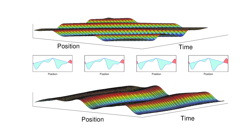
Figure 1: At the top, a representative schematic of a system evolving in space and time. Here, the domain is periodic in the spatial direction. Using a triangle shape as a template (see text for a discussion of templates), we spatially shift each dynamic snapshot (each time slice of the top figure) to maximally correlate with the triangular template. Four such maximal correlations are shown in the middle figure, where the shading brings out the difference between the snapshot and the template. At the bottom, we see that after alignment, the dynamics of the set of snapshots appears visually much simpler; the traveling motion is gone, and all that remains is a slight modulation.

The removal of this degree of freedom allows us to perform certain tasks, such as denoising a collection of snapshots through averaging (in Singer et al. ; Singer & Shkolnisky , a similar procedure is used on cryo-EM data), more easily. In the case where $u(\theta,t)$ is evolving its shape in addition to traveling (for example, when $\mathcal{D}(u)=\omega u_{\theta}+\mathcal{E}(u)$, where $\mathcal{E}(u)$ is some other nonlinear spatially invariant operator), removing this “traveling” degree of freedom from the simulation can significantly assist our understanding of the dynamics. See Figure 1 for an illustration. For instance, when one uses diffusion maps to explore whether the simulation data are intrinsically low-dimensional, and to find good “coarse” parametrizations for them (see, e.g., Lafon & Lee (2006); Sonday et al. (2009); Das et al. (2006); Coifman et al. (2005b); Erban et al. (2007)), removing the symmetry results in a more parsimonious description of the dynamics (an embedding in a lower-dimensional space), which may also be successfully deduced with far less data.

Now, suppose we have an ensemble of $M$ snapshots, but we do not know the members of the underlying symmetry group with which each snapshot is to be identified. We wish to perform this association of snapshots with symmetry group elements; in other words we wish to globally “align” the $M$ snapshots. (Here the colloquial expression “alignment” comes from the simple conceptual example of rotationally invariant functions on the unit circle; the possible rotation angles can be “strung” along a line between $0$ and $2\pi$.)

Normally, this global alignment (the computation of the symmetry group element identified with each snapshot) may be accomplished numerically through the use of a well-chosen template function (see Figure 1 and, e.g., Ahuja et al. (2007); Rowley & Marsden (2000)). For instance, in our running example of snapshots $\{u(\theta,t_{k})\}_{k=1}^{M}$, one finds the alignments $\{\theta_{k}\}_{k=1}^{M}$ which align each snapshot with a template $T(\theta)$ by simply setting

$$\theta_{k}=\underset{c}{\operatorname{argmin}}\,\,\|T(\theta)-u(\theta+c,t_{k})\|^{2}.$$ (3)

The analogue of equation (3) holds for other symmetry groups. This approach will, in general, be successful when

• there is little noise in the data;

• a “good” template, leading to a clear global minimum, is known ahead of time; and

• this template remains “good” in the above sense as new data are collected during the system evolution.

When there is noise in the data, or when a good template is not known, “misalignments” may happen frequently. Furthermore, as the system evolves, a fixed template may stop being “good” (that is, giving rise to a clear global minimum in the above optimization problem).

In this paper we apply a novel spectral algorithm (Singer (2011)) to solve this problem of global alignment in the presence of symmetry. In contrast to the method of templates, which compares snapshots one by one to a fixed “template function” (producing $M$ pieces of information), the eigenvector method compares all snapshots to all other snapshots pairwise, in essence treating every snapshot as a template (and thereby exploiting a greater amount of information, namely $M(M-1)/2$ pieces). Even though many of these pairwise comparisons may be inaccurate due to noise inherent in the snapshots, consistency relationships among these pairwise alignments can be used to gain a sense of the overall, global alignment. A slight modification of this algorithm known as vector diffusion maps (Singer & Wu ) allows for the situation in which the snapshots differ not only by a symmetry group element (and noise), but also because there is a systematic change in the snapshots due to the underlying dynamic evolution. Both algorithms are fast, simple, and (as we will demonstrate) more robust to noise than their corresponding template-based approaches.

The “eigenvector algorithm” will be illustrated through two prototypical examples. The first involves the evolution of orientational distribution functions of nematic liquid crystal polymers; the distributions are functions on the sphere, and we take the associated symmetry group to be $SO(3)$. The second involves spatiotemporally traveling/modulating waves of the Kuramoto-Sivashinsky equation (KSE); these are functions on the unit circle with periodic boundary conditions, and we take the associated symmetry group to be $SO(2)$. Additionally, for the case of the KSE waves, we demonstrate the use of vector diffusion maps to (all in a single step), remove the underlying symmetry and capture the low-dimensionality of the underlying dynamics (the residual dynamics of modulation after the “traveling” symmetry has been removed).

3 The eigenvector alignment method

In its most general form, the eigenvector alignment method (Singer (2011)) can be summarized as follows. Consider an ensemble of $M$ snapshots which are identical, except for the action of some underlying symmetry group $G$ (such as spatially periodic translation) and perhaps some noise. We wish to know the group elements $\{g_{i}\}_{i=1}^{M}\in G$ with which the $M$ snapshots may be identified; this will give us information which can be used to, for instance, ascertain what “rotation” to perform to make a particular snapshot equivalent to another (i.e. to “align” the two snapshots). Specifically, if we identify snapshots $i$ and $j$ with group elements $g_{i}$ and $g_{j}$, then rotation of snapshot $i$ by $g_{ij}\equiv g_{j}g_{i}^{-1}$ should make it identical to snapshot $j$. In our simple illustration of periodic functions $u(\theta,t)$ traveling around the circle with speed $\omega$ (dynamics $u_{t}=\omega u_{\theta}$), the symmetry group elements are angles modulo $2\pi$ (the group is $SO(2)$). Each snapshot $u(\theta,t_{i})$ can, in principle, be identified with some angle $\theta_{i}$. Snapshot $i$ may be made equivalent to snapshot $j$ after a (say, systematically counter-clockwise) rotation of snapshot $i$ by $\theta_{ij}\equiv\theta_{j}-\theta_{i}$.

When the snapshots are noise-free, obtaining the $\{g_{i}\}_{i=1}^{M}$ may be done easily as follows. Choose one base snapshot, or “template,” say snapshot $i$. For this snapshot $i$, choose a particular random assignment $g_{i}$. For each remaining snapshot $j$, find the $g_{ij}\in G$ which rotates snapshot $i$ to be identical to snapshot $j$, and then set $g_{j}=g_{ij}g_{i}$. Alignments between any two snapshots $p$ and $q$ can then be computed as $g_{pq}=g_{ip}^{-1}g_{iq}$. In the example of angles modulo $2\pi$, this means choosing some base $\theta_{i}$ for snapshot $i$, then setting $\theta_{j}$ (for each of the remaining snapshots) to be $\theta_{j}=\theta_{ij}+\theta_{i}$ (where $\theta_{ij}$ is the angle which rotates snapshot $i$ to be identical to snapshot $j$). Alignments between any two snapshots $p$ and $q$ can then be computed as $\theta_{pq}=\theta_{iq}-\theta_{ip}$ (to get from snapshot $p$ to $q$, rotate snapshot $p$ back to snapshot $i$, then rotate $i$ to $q$).

Because the method above relies on using only a single template, it may well not be robust to noise; obtaining the $g_{j}$ may not work well because many of the $\{g_{ij}\}_{j=1}^{M}$ will be computed incorrectly. The eigenvector method instead has the user compute all $\{g_{ij}\}_{i,j=1}^{M}$ (in essence, treating every snapshot as a template); it then looks for consistency along these pairwise alignments to assign the global alignments $\{g_{i}\}_{i=1}^{M}$. The main idea is as follows: if $g_{ij}$, $g_{jk}$, and $g_{ik}$ are accurately measured, we also expect, for example, that

$$g_{ik}=g_{ij}g_{jk},$$ (4)

a condition known as the triplet consistency relation. In our example of angles modulo $2\pi$, this simply says that, regardless of whether snapshot $i$ or $j$ are used as the template, the angle between snapshot $i$ and snapshot $k$ should be the same no matter if it is measured directly ($\theta_{ik}$) or inferred ($\theta_{ij}+\theta_{jk}$). Analogously, we also expect “higher-order” consistency relations of the form

$$g_{il}=g_{ij}g_{jk}g_{kl}.$$ (5)

Since many of the measurements of $g_{ij}$ may be inaccurate, equations (4), (5), and their high-order forms will often be violated; however, one can still hope to assign the $g_{i}$ in some sort of globally optimally consistent way.

Initially, one may attempt to assign the $g_{i}$ so that as many pairwise measurements $g_{ij}$ as possible are satisfied to within some tolerance. Unfortunately, for even a moderate number of group elements $M$, it is computationally intractable to find the assignment of the $g_{i}$ which maximizes the number of them which are satisfied (to within some tolerance). This is a non-convex optimization problem in a very high dimensional space. As we discuss now on the example of angles modulo $2\pi$, a relaxation of the problem to a quadratic (and therefore convex) form has been proposed (Singer (2011)). The only requirement is for the symmetry group $G$ to have a compact real/complex form. The relaxation makes the optimization problem more tractable, but it also allows for the “solution” $g_{i}$ to include elements not necessarily in $G$ (we will explain this and show how it can be rectified below).

Again, consider the problem of angles modulo $2\pi$. This group has a compact complex representation given by mapping $\theta_{i}$ to $e^{i\theta_{i}}$. Measurements of $\theta_{ij}$, which are (noisy) measurements of $\theta_{j}-\theta_{i}$, are represented similarly as $e^{i\theta_{ij}}$. At first, one might wish to formulate the problem so as to assign the global alignments $\theta_{i}$ in order to maximize the number of pairwise measurements which hold true to within some tolerance tol, for instance

$$\underset{\{\theta_{i}\}}{\operatorname{argmax}}\,\,\#\{(i,j):\,\,-\mbox{tol}\leq\theta_{j}-\theta_{i}-\theta_{ij}\,\,(\mbox{mod}\,\,2\pi)\leq\mbox{tol}\}.$$ (6)

This problem becomes quickly computationally intractable for large $M$, even after a reformulation to the form

$$\underset{\{\theta_{i}\}}{\operatorname{argmin}}\,\,\sum_{(i,j)}f\left[\theta_{j}-\theta_{i}-\theta_{ij}\,\,(\mbox{mod}\,\,2\pi)\right],$$ (7)

where $f$ is some smooth periodic penalty function.

Instead, the problem is relaxed as follows: the measurements $\theta_{ij}$ are inserted into a matrix $\mathbf{H}$ so that $\mathbf{H}_{ij}=e^{-i\theta_{ij}}$. We now consider maximizing the following quantity:

$$\underset{\{\theta_{i}\}}{\operatorname{argmax}}\,\,\sum_{i,j}^{M}e^{-i\theta_{i}}\mathbf{H}_{ij}e^{i\theta_{j}}.$$ (8)

When the $\theta_{i}$ are correctly assigned, each “good” measurement of $\mathbf{H}_{ij}$ contributes close to $1$ in the sum and each “bad” measurement contributes, on average, $0$ to the sum (since the errors are assumed to be uniformly randomly distributed, see Singer (2011)). Therefore, the maximization of the expression (8) is likely to produce, in some sense, maximally consistent assignments of the $\theta_{i}$. To make the problem even more tractable, it is further relaxed to a quadratic form (general complex numbers, as opposed to complex numbers on the unit circle only) which can be easily solved with power iteration:

$$\underset{\{z_{i}\}\in\mathbb{C},\sum|z_{i}|^{2}=M}{\operatorname{argmax}}\,\,\sum_{i,j}^{M}z_{i}^{*}\mathbf{H}_{ij}z_{j}.$$ (9)

Maximizing the expression (9) amounts to finding the largest eigenvector $v$ of the Hermitian matrix $\mathbf{H}$. The components of the largest eigenvector $v$ are not necessarily of unit length, but after normalization, one can define the estimated angles by

$$e^{i\theta_{i}}=\frac{v(i)}{|v(i)|}.$$ (10)

It is interesting to note that the error of the assignments $\theta_{i}$ can be estimated by looking at the eigenvalue spectrum of $\mathbf{H}$. Consider, for instance, the correlation $\rho$ between the eigenvector $v$ and the vector $z$ of true angles as a measurement of “goodness of fit”; this is given as

$$\rho=\left|\frac{1}{\sqrt{M}}\sum_{i=1}^{M}e^{-i\theta_{i}}v(i)\right|=|\langle z,v\rangle|.$$ (11)

Under certain assumptions about the type of noise in the problem, one can show that

$$\left|\langle z,v\rangle\right|^{2}\geq\frac{\lambda_{H}-\lambda_{R}}{Mp},$$ (12)

where $M$ is as above, and $p$ is a quantity related to how likely “good” measurements are (see Singer (2011) for details). Here $\lambda_{H}$ is the leading eigenvector of the matrix $\mathbf{H}$; if the (random) matrix $\mathbf{H}$ has a number of properties (again, see Singer (2011); Féral & Péché (2007)) its eigenvalue distribution will include a semicircle, and the right edge of this semicircle will be the quantity $\lambda_{R}$. Furthermore,

$$\lambda_{R}\approx 2\sqrt{M(1-p^{2})}$$ (13)

and

$$\mathbb{E}\left[\lambda_{H}\right]\approx Mp+\frac{1-p^{2}}{p},$$ (14)

where equation (14) is valid whenever $p>1/\sqrt{M}$ and the variance in the quantity $\lambda_{H}$ increases as $p$ decreases (Singer (2011); Féral & Péché (2007)).

Although the noise model presented in Singer (2011) is different than the noise in our problems, equation (11) holds regardless, and we still expect the alignment error to decrease as both $M$ and $p$ grow (more data/pairwise comparisons and higher quality measurements, respectively, will lead to a better recovery of the global alignments).

We also note that Féral & Péché (2007) requires the noise in every entry of the matrix $\mathbf{H}$ to be independent. This is not necessarily true in our examples. It is likely that “good” and “bad” measurements are not random, but rather, correlated; having independent entries requires $M^{2}$ sources of randomness, and clearly, for large enough $M$, this will cease to be true because the “amount” of randomness scales only as $M$, the number of snapshots. For large $M$ this argument can rationalize why some eigenvalues (with magnitude of $O(M)$) may appear outside the theoretically expected semicircle (see, e.g., Figures 5 and 15). This phenomenon is investigated in Cheng & Singer .

4 The first illustrative example: orientational distributions of nematic liquid crystal polymers

Symmetry often plays an important role in systems with spontaneous spatiotemporal pattern formation; such systems, typically modeled through partial differential equations, arise naturally in modeling reaction-diffusion and/or flow (Cross & Hohenberg (1993)), but also nonlinear optics (Arecchi et al. (1999)) and Bose-Einstein condensates (Kevrekidis et al. (2008)). If the computational models are in the form of stochastically interacting particles, the finite number of the simulated particles and the stochasticity of their evolution naturally gives rise to noise in the recorded time series (and we know that the fewer the particles, the “larger” in some sense the noise will be). To illustrate this, and to show how to factor out symmetries at the “macroscopic” level while working with a “microscopic,” particle based, noisy simulation, we chose an illustrative example for which good models exist at both the particle- and the continuum levels. The system in question is the evolution of the single particle orientational probability distribution function in the case of nematic liquid crystals; a closed equation that very successfully approximates this evolution is a Smoluchowski equation (Siettos et al. (2003)). An alternative description of the dynamics comes in the form of coupled stochastic differential equations which model the interactions of a (large but) finite number of nematic liquid crystal polymer molecules; one hopes that, for a large enough number of simulated interacting particles, the computed evolution of their collective orientational probability distribution approximates the trajectories of the (mesoscopic) Smoluchowski equation.

It is well known (and can be seen from the form of equation 15 below) that the evolution of the orientational probability distribution is characterized by equivariance: rotating the initial distribution on the unit sphere and evolving commutes with evolving for the same amount of time and then rotating the final distribution. This implies that experiments (or simulations) differing by some (unknown) mesoscopic rotation of the entire initial distribution should, in effect, produce the same results (modulo the effects of noise).

4.1 System setup

Liquid crystalline polymers (LCPs) are large molecules which contain long rigid segments. Groups of LCPs are capable of displaying rich behavior including high modulus in the solid phase, low viscosity in the melt, and many other interesting and/or desirable physical properties. Each LCP can be thought of as a “needle,” whose orientation may be described as a pair of antipodal points $\pm\mathbf{w}$ (the “tips” of the needle) on the unit sphere; as the number of LCPs in a group becomes large, the evolution of the single-particle orientational probability distribution function $\psi(\mathbf{u})$ of the group is accurately described by the Smoluchowski equation

$$\frac{\partial\psi(\mathbf{u})}{\partial t}=D\frac{\partial}{\partial\mathbf{u}}\cdot\left[\frac{\partial\psi(\mathbf{u})}{\partial\mathbf{u}}+\psi(\mathbf{u})\frac{\partial}{\partial\mathbf{u}}\left(\frac{V[\psi,\mathbf{u}]}{kT}\right)\right].$$ (15)

Here, $\mathbf{u}$ is a unit vector describing orientation, $\partial/\partial\mathbf{u}$ is the gradient operator restricted to the unit sphere, k is Boltzmann’s constant, T is the absolute temperature, D is the rotational diffusivity (here set to $1$), and $V[\psi,\mathbf{u}]$ is a nematic potential (a free energy taking into account excluded volume effects). For our simulations, we use the Maier-Saupe potential (see, e.g. Maier & Saupe (1959))

$$V[\psi,\mathbf{u}]=-\frac{3}{2}U\mathbf{u}\mathbf{u}:\mathbf{S},$$ (16)

where $\mathbf{S}=\langle\mathbf{u}\mathbf{u}\rangle-\frac{1}{3}\mathbf{I}$ is the tensor order parameter. The parameter $U$ (the intensity of the nematic potential) can be thought of as proportional to the concentration of the LCP “rods”. If $\lambda$ is the eigenvalue of $\mathbf{S}$ with the largest magnitude, the so-called scalar order parameter $S$ is given by $S=3\lambda/2$ (Siettos et al. (2003)). Writing equation (15) as $\partial\psi(\mathbf{u})/\partial t=\mathcal{D}(\psi(\mathbf{u}))$, the Smoluchowski equation is equivariant in the sense that $\mathcal{D}(\psi(\mathbf{R}\mathbf{u}))=\mathbf{R}\mathcal{D}(\psi(\mathbf{u}))$, where $\mathbf{R}$ is a member of $SO(3)$.

Computationally, the evolution of the distribution function can be simulated as a large set of coupled stochastic differential equations. One simply represents the distribution $\psi(\mathbf{u})$ as a collection of $N$ representative individual LCPs, and then computes their trajectories $\{\pm\mathbf{w}_{i}(t)\}_{i=1}^{N}$ (here, $\{\pm\mathbf{w}_{i}(t)\}_{i=1}^{N}$ are vectors on the surface of the sphere, and the “$\pm$” is because each LCP is really a rod with identical “top” and antidiametric “bottom”). Initializing a distribution $\psi_{0}(\mathbf{u})$ with $N$ particles may be done with the Metropolis-Hastings algorithm (see Metropolis et al. (1953) or the Appendix), and as $N$ goes to infinity, this initialization converges in measure to $\psi_{0}(\mathbf{u})$. Using the $N$ particle trajectories, ensemble averages $\langle f(\mathbf{u}(t))\rangle$ at any time $t$ may be evaluated as $\frac{1}{2N}\sum_{i=1}^{N}f(\mathbf{w}_{i}(t))+f(-\mathbf{w}_{i}(t))$ (where here, again, we have a “$-$” due to the fact that each LCP has a top and a bottom). The distribution $\psi_{t}(\mathbf{u})$ at time $t$ may also be reconstructed by a variety of techniques; here we choose to do the reconstruction by evaluating ensemble averages of the form $\frac{1}{2N}\sum_{i=1}^{N}Y_{l}^{m*}(\mathbf{w}_{i}(t))+Y_{l}^{m*}(-\mathbf{w}_{i}(t))$ (these $Y_{l}^{m*}$ are the spherical harmonics coefficients of $\psi_{t}(\mathbf{u})$, see Section 4.3). The explicit Euler-Maruyama integration of each individual (stochastic) trajectory takes the form

$$\mathbf{w}_{i}(t+\Delta t)=\frac{\mathbf{w}_{i}(t)-\frac{D}{kT}\frac{\partial V}{\partial\mathbf{u}}\Delta t+\sqrt{2D\Delta\mathbf{b}}}{\left|\left|\mathbf{w}_{i}(t)-\frac{D}{kT}\frac{\partial V}{\partial\mathbf{u}}\Delta t+\sqrt{2D\Delta\mathbf{b}}\right|\right|}.$$ (17)

By using different numbers for $N$, the errors in the initialization of $\psi_{0}(\mathbf{u})$, the computations of the $\langle f(\mathbf{u}(t))\rangle$, and the reconstruction (from the particles) of $\psi_{t}(\mathbf{u})$ can be controlled, since they scale as $1/\sqrt{N}$.

The evolution of the Smoluchowski equation is equivariant under the group $SO(3)$; rotating a given orientational probability distribution by some element $\mathbf{R}$ of $SO(3)$ and evolving is the same as evolving first, and then rotating the result by the same group element. In an SDE reformulation of the problem, an orientational probability distribution is represented by $N$ particles. For purposes of computational exploration of its evolution, a particular ensemble of $N$ particles is equivalent to any other ensemble in which each of the $N$ particles $\mathbf{w}_{i}$ is rotated by the same element of the $SO(3)$ group, $\mathbf{w}_{i}\rightarrow\mathbf{R}\mathbf{w}_{i}$. Furthermore, due to the randomness of the Metropolis-Hastings algorithm, each initialization of $\psi_{0}(\mathbf{u})$ leads to a different initial ensemble of $N$ particles (which will accurately represent $\psi_{0}(\mathbf{u})$ as $N$ goes to infinity, but which represent $\psi_{0}(\mathbf{u})$ noisily for finite $N$). Thus, in the limit of infinite $N$, a particular ensemble of $N$ particles initialized consistently with a particular initial probability distribution $\psi_{0}(\mathbf{u})$ is equivalent to another ensemble initialized consistently with $\psi_{0}(\mathbf{R}\mathbf{u})$: the original distribution, but rotated by a member of $\mathbf{R}$ of the $SO(3)$ group. For finite $N$, there is noise, and these two ensembles of $N$ particles are only approximately the same after rotation by a member of $SO(3)$. Finding this corresponding member $\mathbf{R}$ of $SO(3)$ becomes increasingly difficult as $N$ gets smaller.

Suppose we are given a set of $M$ LCP ensembles, each initialized with $N$ particles, each consistently with $\psi_{0}(\mathbf{R}_{i}\mathbf{u})$ for some unknown rotation $\{\mathbf{R}_{i}\}_{i=1}^{M}\in SO(3)$; and let us evolve each of these ensembles for some fixed time $T$. The result is a set of $M$ ensembles of $N$ particles which should be approximately the same after each is rotated by $\mathbf{R}_{i}^{-1}=\mathbf{R}_{i}^{T}\in SO(3)$ (the difference is due to the finiteness of $N$). We wish to be able to consistently determine the unknown members $\{\mathbf{R}_{i}\}_{i=1}^{M}$ so that we know how to relate each ensemble of $N$ particles to each other ensemble. When $N$ is small (equivalently, when the “noise” is large), misalignments are bound to occur frequently. Therefore, as before, we expect the eigenvector alignment method to outperform a method based simply on a fixed template function.

4.2 Consistent initialization of LCP distributions

In order to compare the performance of the eigenvector alignment method with that of the classic template method, we must first generate appropriate data. For chosen $M$ (number of ensembles) and $N$ (number of particles), this can be accomplished by first generating $M$ random members $\{\mathbf{R}_{i}\}_{i=1}^{M}$ of $SO(3)$, and then initializing $M$ ensembles of $N$ particles according to the distributions $\psi_{0}(\mathbf{R}_{i}\mathbf{u})$ via the (random) Metropolis-Hastings algorithm.

This is illustrated through four plots in Figure 2; here, we have plotted both the “top” and “bottom” (which are interchangeable) of each of the $N$ LCP particles. For two random rotation matrices $\mathbf{R}_{1}$ and $\mathbf{R}_{2}$, and for both $N=50$ and $N=5000$, we show initializations with respect to the probability distribution functions $\psi_{0}(\mathbf{R}_{1}\mathbf{u})$ and $\psi_{0}(\mathbf{R}_{2}\mathbf{u})$. Here, we selected and initial probability distribution which resembles a “P” shape (along with its reflection through the origin). It is given by

$$\psi_{0}(\mathbf{u}=(x,y,z))=\frac{1}{\mbox{Norm}}\left\{\begin{array}[]{lr}50/51&z\geq 0\mbox{ and }|x|\leq 0.1\mbox{ and }y\leq 1/\sqrt{2}\\ 50/51&z\leq 0\mbox{ and }|x|\leq 0.1\mbox{ and }y\geq-1/\sqrt{2}\\ 50/51&z,y\geq 0\mbox{ and }0.4\leq\sqrt{x^{2}+y^{2}}\leq 0.6\\ 50/51&z,y\leq 0\mbox{ and }0.4\leq\sqrt{x^{2}+y^{2}}\leq 0.6\\ 1/51&\mbox{else}\end{array}\right.,$$ (18)

where Norm is some normalization so that $\psi_{0}$ integrates to $1$. We subsequently evolved these four ensembles for a fixed amount of time $T$ using the algorithm (17). The resulting ensembles are shown in Figure 3.

Figure 2: Initial distributions of four LCP ensembles from two different rotation matrices (top and bottom rows, $\mathbf{R}_{1}\mathbf{u}$ and $\mathbf{R}_{2}\mathbf{u}$), and with two different numbers of points ($N=5000$ left, $N=50$ right). Shown are both the “top” and “bottom” (interchangeable) of each LCP particle.

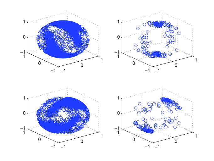
Figure 3: The final distributions after integration by $T=.1$s of the LCP ensembles initialized as in Figure 2. Shown are both the “top” and “bottom” (interchangeable) of each LCP particle.

In the numerical experiments to follow, we choose various values of both $M$ and $N$, thereby generating $M$ different ensembles of $N$ particles corresponding to $\psi_{0}(\mathbf{R}_{1}\mathbf{u})$, $\psi_{0}(\mathbf{R}_{2}\mathbf{u})$, $\ldots$, $\psi_{0}(\mathbf{R}_{M}\mathbf{u})$. We then integrated each ensemble for a fixed amount of time $T$ using the Euler-Maruyama scheme (see equation (17)), obtaining $M$ distributions corresponding to $\psi_{T}(\mathbf{R}_{1}\mathbf{u})$, $\psi_{T}(\mathbf{R}_{2}\mathbf{u})$, $\ldots$, $\psi_{T}(\mathbf{R}_{M}\mathbf{u})$. These distributions differ by (a) a rotation; (b) the particular consistent initialization of the $N$ particles; and (c) the particular (stochastic) particle sample paths computed through the Euler-Maruyama integration.

Given only the noisy particle distributions obtained at time $T$, we wish to determine the $M$ unknown rotation matrices $\mathbf{R}_{1},\mathbf{R}_{2},\ldots,\mathbf{R}_{M}$. When $N$ is small, the noise (which scales as $1/\sqrt{N}$) makes this particularly challenging.

4.3 Alignment of LCP distributions

Pairwise alignment was performed by both the template method (alignment of each ensemble member with a fixed template) and by the eigenvector method (alignment of each ensemble member with each other ensemble member). In our work, we utilized the spherical harmonics components of the orientational distribution functions (computed based on the particle states) to perform pairwise alignment of every pair of ensembles of $N$ representative particles. Akin to a Fourier basis on the sphere, spherical harmonics take into account not only lower-order information such as the center of mass of the distribution (the first three nontrivial spherical harmonics), but also its higher-order moments. Additionally, the leading spherical harmonics coefficients can be used to quickly compare functions and rotated versions of these functions on the sphere (see below), so they are useful for finding optimal pairwise alignments (required by the eigenvector alignment method).

To align two ensembles of $N$ particles, we first approximated computationally the leading coefficients of the spherical harmonics expansion of both particle distributions. Let the spherical harmonics expansion of the first distribution be (approximately) given by

$$f(\theta,\phi)=\sum_{l=0}^{l_{\mbox{max}}}\sum_{m=-l}^{l}f_{l}^{m}Y_{l}^{m}(\theta,\phi).$$ (19)

Here, $f_{l}^{m}$ is computed as an integral over the surface of the sphere $\Omega$ via

$$f_{l}^{m}=\int_{\Omega}f(\theta,\phi)Y_{l}^{m*}(\theta,\phi)d\Omega;$$ (20)

by representing the particles as delta functions, equation (20) is approximated as

$$f_{l}^{m}=\frac{1}{2N}\sum_{i=1}^{N}Y_{l}^{m*}(\theta_{i},\phi_{i})+Y_{l}^{m*}(\pi-\theta_{i},\phi_{i}+\pi),$$ (21)

where $\theta_{i}$ and $\phi_{i}$ are the $(\theta,\phi)$ spherical coordinates of the $i$th particle’s orientation vector $\mathbf{w}_{i}$ in the distribution (and we include $(\pi-\theta_{i},\phi_{i}+\pi)$, of course, because each LCP has a top and bottom which are interchangeable). It is clear that only the even spherical harmonics coefficients survive; for the odd ones, $Y_{l}^{m*}(\theta_{i},\phi_{i})$ $+$ $Y_{l}^{m*}(\pi-\theta_{i},\phi_{i}+\pi)$ equals zero. Similarly, second distribution $g(\theta,\phi)$ may be approximately described by its coefficients $g_{l}^{m}$.

The squared $L^{2}$ difference $\mathbf{e}(f,g)$ between the two functions can then be approximated as

$$\mathbf{e}(f,g)=\sum_{l=0}^{l_{\mbox{max}}}\sum_{m=-l}^{l}||f_{l}^{m}-g_{l}^{m}||^{2}.$$ (22)

Once the spherical harmonics expansion of a function $h(\mathbf{u})$ is known, the spherical harmonics expansion of $h_{\mathbf{R}}\equiv h(\mathbf{R}\mathbf{u})$ can be computed quickly; therefore, it is only necessary to perform the time-consuming calculations in equations (19) and (20) once (these might be sped up by FFT-type fast algorithms which we did not use, see, e.g. Rokhlin & Tygert (2006)). In order to find the rotation matrix $\mathbf{R}$ that best aligns two distributions of $N$ particles with respect to $L^{2}$, we may simply compute

$$\mathbf{R}=\underset{{\mathbf{R}\in SO(3)}}{\operatorname{argmin}}\,\,\mathbf{e}(f,g_{\mathbf{R}}).$$ (23)

Our rotations of the spherical harmonics were performed using the freely available software archive SHTOOLS available at www.ipgp.fr/~wieczor/SHTOOLS, and we computed the best $\mathbf{R}$ by exhaustively searching over $SO(3)$ with a mesh of two degrees precision in each of the $\theta,\phi$ directions. We thus obtained a good initial guesses, for each snapshot, of the sought rotations, and subsequently used Newton iteration to more accurately determine the optimal $\mathbf{R}$.

4.4 Template-based alignment attempts

Using the spherical harmonics machinery, we first attempt to align the set of $M$ ensembles of $N$ particles through the use of fixed templates. Somewhat arbitrarily, we chose the three fixed templates shown in Figure 4. One of the template functions (Template $|-$) resembles the orientational distributions of Figures 2 and 3; we anticipate that at least this template will be useful in aligning the data. Nevertheless, the global alignments obtained with all three fixed templates fall short of those obtained with the eigenvector method (see Table 1).

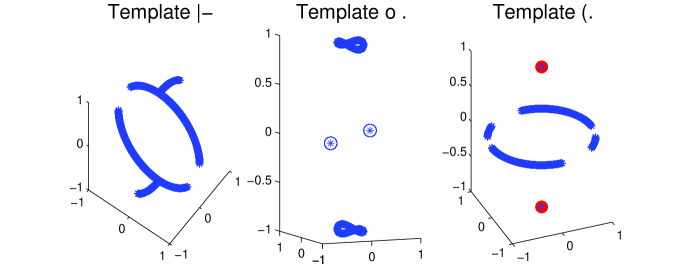
Figure 4: The three templates utilized for alignment of the ensembles of $N$ particles. Because Template $|-$ is vaguely reminiscent of the orientational distributions of Figures 2 and 3, it is expected that it may do well (the “matched filter” is mathematically optimal, see Papoulis (1977)). Nevertheless, it drastically underperforms the eigenvector method, along with the other two templates (see Table 1). Template o . consists of two ellipses (one centered at each pole of the unit sphere) with minor and major axes of $.2$ and $.4$, respectively, along with two points at $(\pm 1/\sqrt{2},\pm 1/\sqrt{2},0)$, each with “mass” equal to one-quarter of the mass of the entire shape. The red dots in Template ( . represent points with infinite weight and are located at $(0,0,\pm 1)$; the effect is that each snapshot is first rotated so that its center of mass lies along the z-axis, and then it is rotated along this axis (an $SO(2)$ rotation) to optimally align with the broken semicircle “(” shape.

4.5 Application of the eigenvector method

The first step in aligning the data through the eigenvector method is to compute pairwise alignments (methodology discussed in Section 4.3) between all $M$ distributions, $\{\mathbf{R_{ij}}\}_{i,j=1}^{M}$. Here, $\mathbf{R}_{ij}$ is the $3\times 3$ matrix which rotates ensemble $j$ to ensemble $i$. Next, these pairwise rotations are inserted in a large $3M\times 3M$ matrix of the following form:

$$\mathbf{M}=\left[\begin{array}[]{cccc}\mathbf{R}_{11}&\mathbf{R}_{12}&\cdots&\mathbf{R}_{1M}\\ \mathbf{R}_{21}&\mathbf{R}_{22}&\cdots&\mathbf{R}_{2M}\\ \vdots&\vdots&\ddots&\vdots\\ \mathbf{R}_{M1}&\mathbf{R}_{M2}&\cdots&\mathbf{R}_{MM}\end{array}\right].$$ (24)

In an ideal setting with no misalignments and no noise, the $ij$-th block of the matrix $\mathbf{M}$ would simply be $\mathbf{R}_{i}\mathbf{R}_{j}^{T}$, for this is the matrix which takes distribution $j$ back to the standard axes, and then rotates it by $\mathbf{R}_{i}$ in order for it to coincide with distribution $i$. We also note that in this ideal setting, the following equation holds:

$$\mathbf{M}\mathbf{v}=M\mathbf{v},$$ (25)

where $\mathbf{v}$ is the $3M\times 3$ matrix

$$\mathbf{v}=\left[\begin{array}[]{c}\mathbf{R}_{1}\\ \mathbf{R}_{2}\\ \vdots\\ \mathbf{R}_{M}\end{array}\right].$$ (26)

Therefore, the top three eigenvectors of $\mathbf{M}$ (each with eigenvalue $M$) contain information about the “unknown” rotation matrices $\mathbf{R}_{i}$. Here, the matrix $\mathbf{M}$ is of rank $3$, and $\mathbf{M}=\mathbf{v}\mathbf{v}^{T}$. That is, $\mathbf{M}$ has only two distinct eigenvalues: an eigenvalue of $M$ whose multiplicity is $3$, and an eigenvalue of $0$ whose multiplicity is $3M-3$. It is therefore expected that the top three eigenvectors would not be affected too much by noise and misalignments.

When there is some noise, the $\mathbf{v}$ matrix will still be resolved (but now with eigenvalues slightly less than $M$), and we expect to be able to recover the information contained in these columns regarding the rotation matrices $\mathbf{R}_{i}$. The recovery will be, of course, only up to an orthogonal transformation which is an inherent degree of freedom: by specifying only pairwise rotations, one only knows how the distributions look relative to each other. This transformation (in effect, its three associated degrees of freedom) appears in equation (25), for this equation holds not only for $\mathbf{v}$, but also for $\mathbf{v}\mathbf{R}$ for any $\mathbf{R}\in\mbox{SO}(3)$. Due to the noise, each recovered $\mathbf{R}_{i}$ is not exactly a rotation matrix (this phenomenon is analogous to the $z_{i}$ not being necessarily of unit length in equation (9) of Section 3). However, one can find the closest (in Frobenius norm) rotation matrix via the well-known procedure: $\mathbf{R}_{i}\rightarrow\mathbf{U}_{i}\mathbf{V}_{i}^{T}$, where $\mathbf{U}_{i}\mathbf{\Sigma}_{i}\mathbf{V}_{i}^{T}$ is the SVD of $\mathbf{R}_{i}$ (Fan & Hoffman (1955); Keller (1975)).

Because Féral & Péché (2007) requires the noise in each element of the matrix $\mathbf{M}$ to be independent, we do not see the expected semicircle-type distribution in our Figure 5; notice, however, that a shape reminiscent of a semicircle can still be seen. Again, this is due to the fact that “good” and “bad” measurements are not random and independent, but rather, correlated; having independent entries requires $M^{2}$ sources of randomness, and clearly, for large $M$, this is not true because the “amount” of randomness grows only as $M$, the number of snapshots. Because of this, for large $M$, some eigenvalues of $O(M)$ appear outside the semicircle. See Cheng & Singer for details.

The error in the global rotations recovered are shown in Table 1. The eigenvector method appears quite successful: even for large amounts of noise (small $N$) and small values of $M$, favorable results are obtained. Even though the eigenvalue semicircle analysis of Section 3 was carried out for group $SO(2)$ and not the group $SO(3)$ of interest here, the distance from the leading eigenvector to the noisy semicircle still quantifies the alignment error. Furthermore, as expected, when both $M$ and $N$ both become large (large $N$ means that the probability of “good” measurements goes up, and in the context of Section 3, that $p\rightarrow 1$), the leading eigenvalues ($\lambda_{H1},\lambda_{H2},\lambda_{H3}$) increase as $O(M)$ and the position of $\lambda_{R}$ increases as $O(\sqrt{M})$. These results are summarized in Table 1.

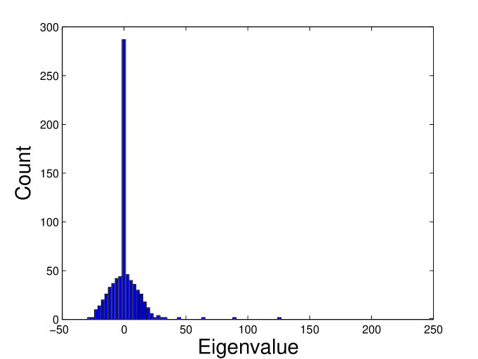
Figure 5: A histogram for the eigenvalues for $M=250$ and $N=10$. One eigenvalue is near $250$, and there are four pairs of eigenvalues near $125$, $88$, $63$, and $44$ (these are likely due to the correlations in the matrix $\mathbf{M}$, see Cheng & Singer and Section 3). The other eigenvalues are “in the semicircle.” We need the largest three eigenvalues and their eigenvectors to recover the rotations. So, in practice we use the eigenvalue near $250$ and the pair of eigenvalues near $125$.

$N$	$M$	$\lambda_{H1}$	$\lambda_{H2}$	$\lambda_{H3}$	$\lambda_{R}$	$\mbox{err}_{\lambda}$	$\mbox{err}_{|-}$	$\mbox{err}_{o.}$	$\mbox{err}_{(.}$
	$250$	$249.9$	$182.9$	$182.9$	$22.2$	$0.078$
	$125$	$125.0$	$91.2$	$91.2$	$18.1$	$0.125$
$5000$	$63$	$63.0$	$47.8$	$47.8$	$11.7$	$0.189$	$1.3671$	$2.0801$	$1.7671$
	$32$	$32.0$	$23.6$	$23.5$	$7.9$	$0.196$
	$16$	$16.0$	$13.0$	$13.0$	$4.6$	$0.204$
	$250$	$249.9$	$179.2$	$179.2$	$24.3$	$0.110$
	$125$	$125.0$	$89.9$	$89.9$	$19.6$	$0.135$
$1000$	$63$	$63.0$	$44.8$	$44.7$	$14.4$	$0.197$	$1.4339$	$2.2302$	$1.9340$
	$32$	$32.0$	$23.4$	$23.3$	$8.6$	$0.225$
	$16$	$16.0$	$12.8$	$12.8$	$5.9$	$0.351$
	$250$	$249.9$	$175.9$	$175.9$	$25.8$	$0.181$
	$125$	$125.0$	$88.2$	$88.1$	$19.7$	$0.193$
$200$	$63$	$63.0$	$44.4$	$44.4$	$14.6$	$0.257$	$1.4398$	$2.4334$	$1.9420$
	$32$	$32.0$	$23.3$	$23.3$	$9.4$	$0.303$
	$16$	$16.0$	$12.8$	$12.8$	$6.5$	$0.358$
	$250$	$249.9$	$146.2$	$146.2$	$36.2$	$0.403$
	$125$	$124.9$	$75.6$	$75.6$	$19.9$	$0.412$
$50$	$63$	$63.0$	$39.0$	$39.0$	$15.3$	$0.535$	$1.4419$	$2.5908$	$2.0040$
	$32$	$32.0$	$21.2$	$21.1$	$10.2$	$0.624$
	$16$	$16.0$	$9.9$	$9.9$	$9.9$	$0.780$
	$250$	$248.8$	$125.1$	$125.1$	$37.2$	$0.604$
	$125$	$124.9$	$63.2$	$63.2$	$21.5$	$0.836$
$20$	$63$	$63.0$	$31.7$	$31.7$	$19.3$	$0.862$	$1.4475$	$2.6133$	$2.0084$
	$32$	$32.0$	$17.8$	$17.8$	$10.3$	$0.988$
	$16$	$16.0$	$9.6$	$9.6$	$10.2$	$1.087$
	$250$	$249.7$	$124.2$	$124.1$	$38.8$	$1.148$
	$125$	$124.8$	$61.8$	$61.7$	$22.4$	$1.192$
$10$	$63$	$62.9$	$30.0$	$30.0$	$22.0$	$1.195$	$1.5413$	$2.6156$	$2.3441$
	$32$	$31.9$	$16.9$	$16.9$	$11.1$	$1.263$
	$16$	$16.0$	$8.9$	$8.9$	$10.9$	$1.459$

Table 1: Results of the eigenvector method (vs. $N$ and $M$) and alignments with various templates (vs. $N$). As before, $N$ is the number of LCP particles representing the distribution (smaller $N$ implies more noise). $M$ is the number of ensembles of $N$ particles, meaning that we perform $M(M-1)/2$ comparisons when using the eigenvector method. $\lambda_{H1}$, $\lambda_{H2}$, and $\lambda_{H3}$ are the $3$ largest eigenvalues of the $3M\times 3M$ matrix $\mathbf{M}$, and these are the eigenvalues which contain the rotation matrix information. $\lambda_{R}$ is the eigenvalue at the right edge of the semicircle. Finally, the “err” quantities describe the error in the computed $\mathbf{R}_{i}$, and are equal to $1/M\sum_{i=1}^{M}\|\mathbf{R}_{i\,true}-\mathbf{R}_{i}\|_{F}^{2}$ ($\mbox{err}_{\lambda}$ is for the eigenvector method, and the rest are for the templates shown in Figure 4). The eigenvector method easily outperforms all templates, and as expected, the error grows as $M$ and $N$ get smaller due to less information and more noise, respectively. $\lambda_{H1}$ appears to scale as $M$, while $\lambda_{H2}$ and $\lambda_{H3}$ scale with $M$ and decrease with noise. $\lambda_{R}$ increases with both noise and $M$ (see Section 3).

5 The second illustrative example: modulated traveling waves of the one-dimensional Kuramoto-Sivashinsky equation

Symmetries play an important role in systems that exhibit spatiotemporal pattern formation (and the evolution equations that model them). When processing experimental or computational data that arise in observing such problems, it again makes sense to first factor out the underlying symmetries. As an example of such a spatiotemporal pattern-forming system, we choose the Kuramoto-Sivashinksy equation (KSE) in one spatial dimension and with periodic boundary conditions, which can be written in the following form:

$$u_{t}+4u_{xxxx}+\alpha[u_{xx}+uu_{x}] = 0,$$

$$u(t,x) = u(t,x+2\pi).$$ (27)

This well-known nonlinear PDE arises as a model in many physical contexts, from flame front propagation to the dynamics of falling liquid films (Sivashinsky (1977); Kuramoto & Tsuzuki (1976)). It gives rise to a rich variety of spatiotemporal dynamical patterns including steady state multiplicity and symmetry-breaking bifurcations, as well as traveling, modulated and “turbulent” waves. It has been shown, under certain conditions, to possess inertial manifolds (Jolly et al. (1990)), implying that its long-term dynamics are low-dimensional; this low dimensionality, along with the rich spatiotemporal dynamics, is an important reason for selecting it as an illustrative example.

5.1 System setup

For certain values of the parameter $\alpha$, the KSE exhibits attractors that are traveling waves that are not of constant shape, but rather exhibit spatiotemporal fluctuations; these are termed Modulated Traveling Waves (MTWs). Such attractors can be thought of as two-dimensional tori ($T^{2}$) in infinite-dimensional space; one “direction” around the torus corresponds to traveling, and the other to a periodic modulation. We will study transient computational data obtained in such a parameter regime; the data do not necessarily lie on the MTW attractors, but they are visually close enough that the two types of motion are visible in our plots.

Equation (27) is equivariant with respect to spatial translations; therefore, the “traveling” behavior of these waves may be factored out (the underlying symmetry group is that of positions $x$ modulo $2\pi$, or, as we referred to it before, that of angles modulo $2\pi$ – $SO(2)$). Writing equation (27) as $u_{t}=\mathcal{D}(u)$, the equivariance relation becomes $\mathcal{D}(S_{c}[v])=S_{c}[\mathcal{D}(v)]$, where $S_{c}[v](x)=v(x+c)$ is the shift operator on spatially periodic functions.

Although the traveling behavior of the wavy transients can be factored out, their modulation cannot. For an exact MTW attractor, where the modulation (as opposed to the traveling) is exactly periodic in time, there does exist a continuous, one-to-one map between each phase of the temporal modulation and the set of points on the circle; yet this does not lead to equivariance. It is the spatial shifts of arbitrary wave profiles (not the temporal ones on exactly periodic attractors) that we are interested in.

An additional qualitative computational observation is that variations in the solution snapshots associated with the traveling component of the evolution are significantly larger than the variations associated with the “modulation” part, which remains after the traveling has been factored out (as will be described below). Based on this observation, we will still use the eigenvector method to align the data, even though in its formulation such a modulation is not taken into account (for a formulation which does take this into account, see the discussion about vector diffusion maps, Section 7, further below). We will compare this to alignments obtained using template-based methods (as was done in Rowley & Marsden (2000)). The output of both methods, the list of global alignments for each wave snapshot, can then be used to align each wave snapshot so that the traveling motion is factored out and we can focus on studying the modulation exclusively (for instance, through the use of diffusion maps). Figure 6 is a picture of (a transient closely approximating) a modulated traveling wave, and Figure 7 shows the temporal evolution of the wave shapes on this transient.

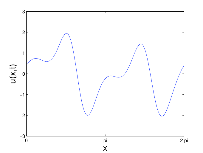
Figure 6: A temporal snapshot (spatial profile at a moment in time) from a PDE solution close to a modulated traveling wave attractor for $\alpha=32$.

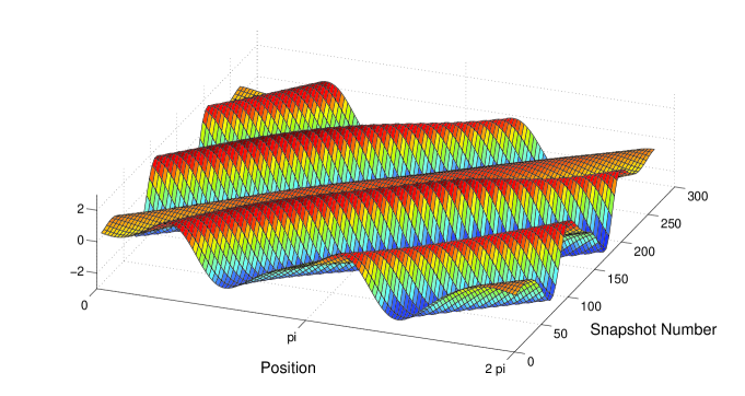
Figure 7: A sequence of MTW snapshots demonstrating the temporal evolution of the MTW. One can clearly see the traveling motion and a slight modulation on top of this motion.

5.2 Generation of snapshot data in the MTW parameter regime

To generate an ensemble of $M$ transient snapshots in the neighborhood of an MTW attractor, we begin by integrating equation (27) for an extended period of time on an evenly spaced grid of $128$ mesh points with width $2\pi/128$. Because the MTW behavior is an attractor for the system, after this long time, each $u(x,t)$ at a fixed time $t$ can be thought of as accurately approximating a snapshot on the MTW. In Figure 7 we show a sequence of such “MTW snapshots”.

We take snapshots $u(x,t_{1}),u(x,t_{2}),\ldots,u(x,t_{M})$ at $M$ different times $t_{1},t_{2},\ldots,t_{M}$. We then make these snapshots artificially noisy by adding Gaussian white noise of variance $\sigma^{2}$ to each of them (to each of the $128$ mesh points $\{x_{i}\}_{i=1}^{128}$, we add a normal random variable of variance $\sigma^{2}$). Without this noise, traditional single template-based approaches can do a very good job of factoring out the traveling motion of the MTW. With this noise, however, template-based approaches can fail spectacularly, while the eigenvector alignment method may still usefully resolve the global alignments.

5.3 Alignment of MTW snapshots

To find the alignment $a_{ij}$ which aligns a (noisy) wave snapshot $u(x,t_{i})$ with another $u(x,t_{j})$, we simply set $a_{ij}$ equal to the $k\in\{1,2,\ldots,128\}$ which minimizes

$$\sum_{l=1}^{128}\left[T_{k}[u](x_{l},t_{i})-u(x_{l},t_{j})\right]^{2};$$ (28)

here $T_{k}$ is the periodic shift operator on the $128$ mesh points $\{x_{i}\}_{i=1}^{1}28$ defined by $T_{k}[u](x_{l},t)=u(x_{k+l},t)$. The analogue of equation (28) is also used to align a (noisy) MTW snapshot against a chosen (fixed) template.

5.4 Template-based alignment attempts

Although it is best to select a template with some prior knowledge, even relatively arbitrary choices (e.g. a “Mexican hat”) may give good results. When the wave snapshots contain more than a little noise, however, alignment with a template will certainly give rise to many incorrect answers. Furthermore, even with no noise, poor template choices may result in spurious alignments.

Figure 8 shows a MTW snapshot with added Gaussian white noise of variance $\sigma^{2}=3.5^{2}$. Clearly, this amount of noise will present a problem to alignment efforts: it is difficult to even visually perceive the resemblance with the noiseless MTW snapshot (Figure 6). Nevertheless, we attempt to align this snapshot (as well as others taken from our data set, with the same type of noise added) using different templates. The next series of figures shows

• on the right, the alignment of each noisy wave snapshot in our data set with a particular single template (obtained by finding the periodic shift which, according to equation (28), results in maximum correlation/minimum $L^{2}$ distance with the fixed template) vs. its correct alignment; ideally, this plot should consist of one straight line (after taking into account periodicity)

• on the left, to demonstrate the degree of robustness of the alignment procedure, a plot of the $L^{2}$ distance between the template function and “all” periodic shifts of a single noisy MTW snapshot randomly chosen from our data set. This function’s minimum is the alignment chosen for this noisy MTW by the template method (it maximizes the correlation/minimizes the $L^{2}$ distance), and it is this “best” alignment for all the snapshots that is plotted in the figure on the right.

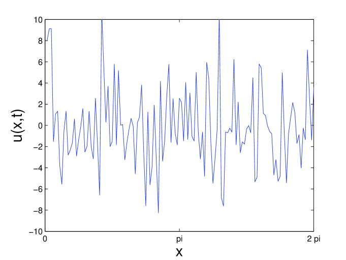
Figure 8: A snapshot of an MTW with Gaussian white noise of variance $3.5^{2}$ added.

First, for reference, the alignment of noiseless snapshots with a template (here, the template was chosen to be a particular noiseless MTW snapshot) would appear like Figure 9. In this figure, as expected, the alignments obtained are nearly perfect (the figure resembles a straight line with small-in the $L^{2}$ norm-“gaps” caused by the modulation, which we will not study further here). These favorable results are expected since we are using a mathematically motivated template (a “matched filter,” see Papoulis (1977)) in noiseless conditions. In a slightly more realistic setting our snapshots will be noisy (and we still use a noiseless MTW snapshot as our template); this result is shown in Figure 10. Again, the alignments obtained are nearly perfect (the small “gaps” also remain), but now there are a few errors. Of course, using a noiseless MTW snapshot as our template can be thought of as slightly “cheating”; from our data set of noisy waves close to an MTW attractor, we do not know what an exact, noiseless MTW snapshot looks like.

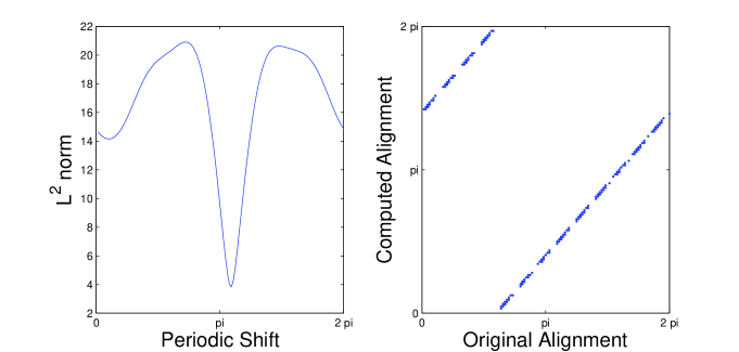
Figure 9: Alignment of noiseless MTW snapshots with a single noiseless MTW as the template. As expected, the alignment appears perfect.

Figure 10: Alignment of noisy MTW snapshots with a single noiseless MTW as the template. The resulting alignment is nearly perfect, but one can see that the robustness of Figure 9 has already started to wane; the range of the $L^{2}$ distances computed in this figure is much narrower than that of Figure 9.

We tried several other template functions, including the Mexican hat, a cosine function, a step function (equivalently, the second Haar wavelet), and a triangle. Voting-based approaches were also tried; in these approaches, the results of multiple templates were averaged together in a suitable way in order to come up with a consensus. These voting-based approaches were also seen to fail; knowing how to average the votes together is a problem, and some templates have many local minima. Finally, center of mass- and moment-based alignment approaches also appeared to fail; this was not unexpected, since aligning based on moments is closely related to template alignmnent. Some of these figures are shown below.

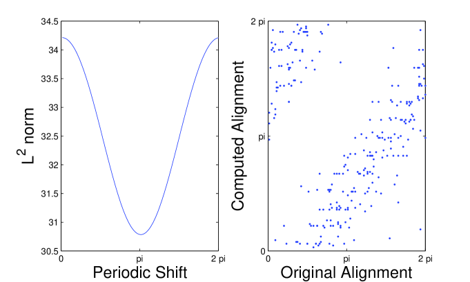
Figure 11: Alignment of noisy MTW snapshots with a cosine. Although the $L^{2}$ distance plot (left) is smooth, its range is much narrower than that of Figure 9 leading to poorer alignments.

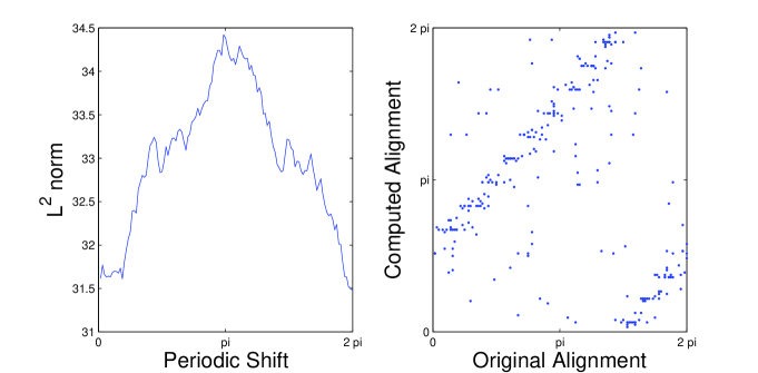
Figure 12: Alignment of noisy MTW snapshots with a step function (the second Haar wavelet). Here, the $L^{2}$ distance plot exhibits a narrow range of values.

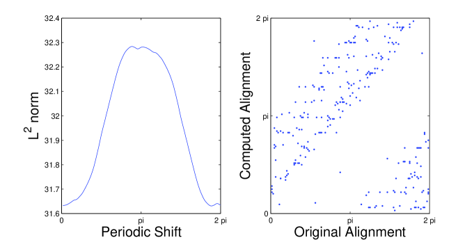
Figure 13: Alignment of noisy MTW snapshots with a triangle-shaped template. As in Figures 11 and 12, the $L^{2}$ distance range is narrow and the alignments obtained are poor.

The only template to give a visually satisfactory answer was a (in principle, unavailable) noiseless MTW snapshot (again, see Figure 10). Since the noiseless MTW template gave such good results, one might be tempted to try a noisy MTW from the data set as a template (which would not be considered cheating!). However, the performance of such a template is spectacularly poor: see Table 2 for summary statistics.

5.5 Application of the eigenvector method

In the presence of so much noise (again, see Figure 8), it is difficult to imagine aligning the noisy wave snapshots without prior knowledge of a good template such as the one provided by a noiseless MTW snapshot (Figure 10). However, the eigenvector method takes into account information based on all pairwise alignments (in essence, treating each wave snapshot as a template, and looking at all $M(M-1)/2$ comparisons) and it is seen to give surprisingly good results.

First, we compute all pairwise alignments between the $M$ noisy wave snapshots by finding the alignment $a_{ij}$ which minimizes the corresponding $L_{2}$ norm of their difference; clearly, many of these may be computed incorrectly. The alignment which rotates snapshot $i$ to snapshot $j$, denoted $a_{ij}$, is (for our spatially discretized waveforms) an integer between $1$ and $128$, describing how many mesh points forward one must shift snapshot $i$ in order for it to maximally correlate with snapshot $j$. This alignment is then mapped to the unit circle via $\mathbf{T}_{ij}=\mbox{exp}(-2i\pi a_{ij}/128)$, and a matrix $\mathbf{T}$ is constructed as follows:

$$\mathbf{T}=\left[\begin{array}[]{cccc}\mbox{exp}(-2i\pi a_{11}/128)&\mbox{exp}(-2i\pi a_{12}/128)&\cdots&\mbox{exp}(-2i\pi a_{1M}/128)\\ \mbox{exp}(-2i\pi a_{21}/128)&\mbox{exp}(-2i\pi a_{22}/128)&\cdots&\mbox{exp}(-2i\pi a_{2M}/128)\\ \vdots&\vdots&\ddots&\vdots\\ \mbox{exp}(-2i\pi a_{M1}/128)&\mbox{exp}(-2i\pi a_{M2}/128)&\cdots&\mbox{exp}(-2i\pi a_{MM}/128)\end{array}\right].$$ (29)

In an ideal setting with no noise/no misalignments, the $ij$-th block of the matrix $\mathbf{T}$ would simply be $\mbox{exp}[-2i\pi/128(a_{j}-a_{i})]$ (where we denote the actual, unknown rotation of snapshot $i$ by $a_{i}$); this is the rotation which takes snapshot $j$ back to the “phase” zero, and then rotates it by $\mbox{exp}(2i\pi a_{i}/128)$ in order for it to coincide with snapshot $i$. We also note that, in this ideal setting, the following equation holds:

$$\mathbf{T}\mathbf{v}=M\mathbf{v},$$ (30)

with

$$\mathbf{v}=\left[\begin{array}[]{c}\mbox{exp}(2i\pi a_{1}/128)\\ \mbox{exp}(2i\pi a_{2}/128)\\ \vdots\\ \mbox{exp}(2i\pi a_{M}/128)\end{array}\right].$$ (31)

The top eigenvector of $\mathbf{T}$ (with eigenvalue $M$) contains, therefore, information about the shifts $a_{i}$ (the “alignments”). In this setting, the matrix $\mathbf{T}$ is of rank $1$, and it satisfies $\mathbf{T}=\mathbf{v}\mathbf{v}^{T}$, so $\mathbf{T}$ has two distinct eigenvalues: an eigenvalue of $M$ whose multiplicity is $1$ and an eigenvalue of $0$ whose multiplicity is $M-1$. It is therefore expected that the top eigenvalue would not be affected too much by noise and misalignments.

When there is some noise, $\mathbf{v}$ will still be approximately resolved (but now with eigenvalue slightly less than $M$), and we are able to recover the information contained in this eigenvector regarding the alignments $a_{i}$. The recovery will be, of course, only up to an overall global shift, which (since we only specify pairwise relative shifts) is an inherent degree of freedom. This can be seen in equation (30); this equation holds for not only $\mathbf{v}$, but also for $\mbox{exp}(i\theta)\mathbf{v}$ (and, in fact, any constant times $v$). In fact, due to the noise, each recovered $a_{i}$ will not have exactly unit magnitude; yet the $a_{i}$ may be recovered by considering both the imaginary and real parts of the $i$th entry of $\mathbf{v}$. In particular, we set

$$a_{i}=\frac{128}{2\pi}\times\mbox{arctan}\left(\frac{\mbox{Im}(\mathbf{v}_{i})}{\mbox{Re}(\mathbf{v}_{i})}\right).$$ (32)

The results of the eigenvector method constitute, without a doubt, a significant improvement upon those obtained using the various fixed templates above (see Figure 14 and Table 2. The eigenvalue distribution can be seen in Figure 15; one large eigenvalue clearly dominates the rest. However, because the theory in Féral & Péché (2007) requires the noise in each of the elements of the matrix $\mathbf{M}$ to be independent, we do not see the predicted semicircle distribution in Figure 15 (although a shape reminiscent of the semicircle can still be discerned). Again, this is due to the fact that “good” and “bad” measurements are not random, but rather, correlated; having independent entries requires $M^{2}$ sources of randomness, and clearly, for large $M$, this is not true because there are only $128\times M$ sources ($M$ snapshots and $128$ random Gaussian variables for each snapshot). Therefore, for large $M$, some eigenvalues of magnitude $O(M)$ appear outside the “semicircle”; see Cheng & Singer for details.

For even larger amounts of noise and even smaller values of $M$, good results can still be obtained. In fact, the distance from the leading eigenvalue to the “noisy semicircle” quantifies the alignment error (see Section 3). When $M$ is large and the problem is relatively noiseless (so that in the context of Section 3, $p\approx 1$), the distance from $\lambda_{H}$ to $\lambda_{R}$ is predicted to be large (again, see Section 3); the position of the leading eigenvalue $\lambda_{H}$ increases as $O(M)$ and the position of $\lambda_{R}$ increases as $O(\sqrt{M})$.

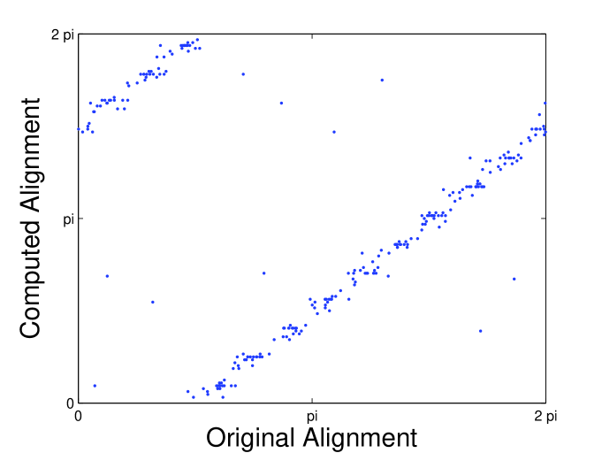
Figure 14: Noisy MTW snapshot alignments obtained using the eigenvector method. A significant improvement upon single template methods is observed.

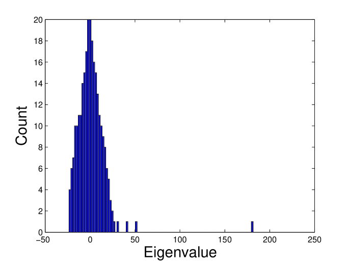
Figure 15: A histogram for the eigenvalues for $M=250$ and $\sigma^{2}=2.5^{2}$. One dominant eigenvalue is near $180$, and there are two others near $50$ (these are likely due to the correlations in the matrix $\mathbf{M}$, see Cheng & Singer and Section 3). The rest of the eigenvalues appear to belong to the “semicircle.”

$\sigma^{2}$	$M$	$\lambda_{H}$	$\lambda_{R}$	$\rho_{\lambda}^{\prime}$	$\rho_{\lambda}$	$\rho_{cos}$	$\rho_{2m}$	$\rho_{tr}$	$\rho_{mh}$	$\rho_{2H}$	$\rho_{M}$	$\rho_{nM}$
	$250$	$248.1$	$9.9$	$1.00$	$1.00$
	$125$	$123.6$	$4.1$	$1.00$	$.999$
$1.0^{2}$	$62$	$60.6$	$2.6$	$.999$	$.999$	$.930$	$.837$	$.779$	$.340$	$.992$	$.999$	$.996$
	$32$	$31.7$	$1.3$	$.999$	$.999$
	$16$	$15.9$	$0.6$	$.999$	$.999$
	$250$	$217.9$	$24.5$	$.994$	$.978$
	$125$	$110.2$	$14.3$	$.993$	$.976$
$2.0^{2}$	$62$	$55.1$	$10.1$	$.993$	$.972$	$.798$	$.556$	$.663$	$.257$	$.846$	$.994$	$.918$
	$32$	$28.3$	$5.4$	$.988$	$.970$
	$16$	$14.0$	$2.3$	$.979$	$.967$
	$250$	$181.9$	$25.1$	$.974$	$.956$
	$125$	$93.9$	$19.4$	$.974$	$.953$
$2.5^{2}$	$62$	$47.2$	$13.8$	$.965$	$.952$	$.757$	$.639$	$.673$	$.272$	$.783$	$.982$	$.882$
	$32$	$24.4$	$9.5$	$.956$	$.946$
	$16$	$13.2$	$6.2$	$.956$	$.946$
	$250$	$124.9$	$30.4$	$.874$	$.868$
	$125$	$61.2$	$21.2$	$.828$	$.836$
$3.5^{2}$	$62$	$33.3$	$14.8$	$.794$	$.832$	$.602$	$.436$	$.504$	$.254$	$.625$	$.909$	$.514$
	$32$	$18.0$	$10.6$	$.771$	$.805$
	$16$	$9.86$	$6.1$	$.698$	$.802$

Table 2: Results of the eigenvector method (vs. $\sigma^{2}$ and $M$) and the alignments with various templates (vs. $\sigma^{2}$). For the eigenvector method, shown are the quantities $\lambda_{H}$ (the largest eigenvalue), $\lambda_{R}$ (the right edge of the semicircle), $\rho_{\lambda}=\left|\frac{1}{\sqrt{M}}\sum e^{-i\theta_{i}}v(i)\right|$, and $\rho_{\lambda}^{\prime}=\left|\frac{1}{M}\sum e^{-i\theta_{i}}\frac{v(i)}{|v(i)|}\right|$. For the template methods, shown are the quantities $\rho=\left|\frac{1}{M}\sum e^{-i\theta_{i}}\mbox{exp}(2i\pi a_{i}/128)\right|$, where the $\theta_{i}$ are the true alignments and the $a_{i}$ are the alignments predicted by various templates: a cosine, the second moment, a triangle, the Mexican hat, the second Haar wavelet, a noiseless MTW snapshot (use of it is “cheating”), and a noisy MTW snapshot (not “cheating”). For a fixed amount of noise, $\lambda_{H}$ appears to increase approximately with $M$, while $\lambda_{R}$ increases approximately with $\sqrt{M}$. As the amount of noise increases ($\sigma^{2}$), $\lambda_{H}$ decreases, $\lambda_{R}$ increases, and, as expected, both of the $\rho_{\lambda}$ decrease (this is expected both intuitively and mathematically, see Section 3). Similarly, other template-based correlations $\rho$ increase with $M$ and decrease with decreasing noise. Clearly, the only competitive template is a noiseless snapshot of the MTW itself.

5.6 Additional denoising procedures

Before concluding this example, we note that if we initially filter the noisy wave snapshots, we observe better performance for both the eigenvector method and for some of the fixed templates. In the Fourier representation of the non-noisy KSE snapshots (convenient for spectral numerical discretization, but also known to be the optimal principal component (PCA) basis for systems with such translational symmetry, see Sirovich (1987)) the power spectrum is known to decay quickly. Therefore, we obtain an increased signal-to-noise ratio by first projecting each noisy wave snapshot onto its Fourier modes with power spectrua larger than some fixed threshold; the information about the underlying (non-noisy) MTW attractor which is thrown away by filtering these Fourier modes is small compared to the noise thrown away by filtering these Fourier modes.

6 Post-processing the aligned data of the Kuramoto-Sivashinsky equation through the use of diffusion maps

In the example of the KSE wave snapshots (Section 5), we conveniently allowed ourselves to ignore the shape modulation superposed to the traveling motion when seeking their global alignments. The reason is that this modulation is comparatively small in $L^{2}$ norm, and therefore, it contributes little to the sum in equation (28). We were able to recover, with good accuracy, the global alignments of the noisy wave snapshots (see Figure 14).

With the global alignments recovered, we rotate each snapshot so that the traveling motion is factored out and only the modulation remains. When there is no noise, the aligned sequence of wave snapshots takes the form of Figure 16 (with noise it is too hard to visually perceive the modulation, so we do not include such a figure).

Figure 16: A sequence of aligned MTW snapshots. In contrast to Figure 7, the traveling has been factored out and only the modulation remains. Although the eigenvector method performs well on noisy snapshots (see, e.g., Figure 14), we chose to show noise-free MTW snapshots for visualization purposes.

Given the aligned data, we now perform diffusion maps in order to search for “coarse variables” (that is, for reduced representations of the data) as in Lafon & Lee (2006); Sonday et al. (2009); Das et al. (2006); Coifman et al. (2005b); Erban et al. (2007)). To construct an informative low-dimensional embedding for this data set of $M$ (noisy but aligned) snapshots, we start with a similarity measure between each pair of snapshots $u(x,t_{i})$, $u(x,t_{j})$. The similarity measure is a nonnegative quantity $\mathbf{W}_{ij}=\mathbf{W}_{ji}$ satisfying certain additional “admissibility conditions” (Coifman et al. (2005a)). Here, we choose the Gaussian similarity measure, and construct a matrix $\mathbf{W}$ as

$$\mathbf{W}_{ij}=\mbox{exp}\left[\frac{\sum_{k=1}^{128}\left[u(x_{k},t_{i})-u(x_{k},t_{j})\right]^{2}}{\varepsilon}\right].$$ (33)

In this equation, $\varepsilon$ defines a characteristic scale which quantifies the “locality” of the neighborhood within which Euclidean distance can be used as the basis of a meaningful similarity measure (Coifman et al. (2005a)). A systematic approach to determining appropriate $\varepsilon$ values is discussed in Grassberger & Procaccia (1983). Next, we create a matrix $\mathbf{K}$ which is a row-normalized version of $\mathbf{W}$:

$$\mathbf{K}_{ij}=\frac{\mathbf{W}_{ij}}{\sum_{l=1}^{M}\mathbf{W}_{il}}.$$ (34)

Finally, we look at the top few eigenvalues and eigenvectors of the matrix $\mathbf{K}$. In MATLAB, for instance, this can be done with the command $[\mathbf{V},\mathbf{L}]=\mbox{eigs}(\mathbf{K},n+1)$, where $n+1$ is the number of top eigenvalues we wish to keep (we typically are only interested in the first few).

This gives a set of real eigenvalues $\lambda_{0}\geq\lambda_{1}\geq...\geq\lambda_{n}\geq 0$ with corresponding eigenvectors $\{\vec{\psi}_{j}\}_{j=0}^{n}$. Since $\mathbf{K}$ is stochastic, $\lambda_{0}=1$ and $\vec{\psi}_{0}=[1\,1\,...\,1]^{T}$. The $n$-dimensional representation of the $i$-th snapshot $u(x,t_{i})$ is given by the diffusion map $\vec{\Psi}_{n}^{(i)}:\,\mathbf{R}^{128}\longrightarrow\mathbf{R}^{n}$, where

$$\vec{\Psi}_{n}\left(u(x,t_{i})\right)=[\lambda_{1}^{t}\vec{\psi}_{1}^{(i)},\lambda_{2}^{t}\vec{\psi}_{2}^{(i)},...,\lambda_{n}^{t}\vec{\psi}_{n}^{(i)}],$$

a mapping which is only defined on the $M$ recorded snapshots. Here, $t$ represents the “diffusion time”; to keep things simple, we choose $t=1$. In other words, snapshot $i$ is mapped to a vector whose first component is the $i$th component of the first nontrivial eigenvector, whose second component is the $i$th component of the second nontrivial eigenvector, etc. If a gap in the eigenvalue spectrum is observed between eigenvalues $\lambda_{n}$ and $\lambda_{n+1}$, then $\vec{\Psi}_{n}$ may provide a useful low-dimensional representation of the data set (Belkin & Niyogi (2003); Nadler et al. (2006)).

When we apply diffusion maps to the (aligned but noisy) wave snapshot data, our eigenvalues are $1.00,\,0.90,\,0.87,\,0.62,\,0.43,\,\ldots$ Clearly, there is a gap between $0.87$ and $0.62$. Therefore, we expect the first two nontrivial eigenvectors to give a parametrization of the residual, “symmetry-adjusted” dynamics corresponding to the modulation. These two eigenvectors are shown in Figure 17. There is a continuous one-to-one map between each possible modulation phase and the set of points on the unit circle, since the data lie very close to the attracting modulated traveling wave, for which the modulation is exactly periodic in time. We thus expect the first two nontrivial eigenvectors to trace out some sort of circle or “loop”; the eigenfunctions of simple diffusion on a closed curve are $\sin(2s\pi/L)$ and $\cos(2s\pi/L)$, where $s$ is some arclength parameter. The eigenvectors shown in Figure 17 do not trace out an exact circle, but the plot is reminiscent of that shape. In fact, by looking at the quantity

$$\tau_{i}\equiv\mbox{arctan}\left(\frac{\vec{\psi}_{2}^{(i)}}{\vec{\psi}_{1}^{(i)}}\right),$$ (35)

we can assign a number $\tau_{i}\in[0,2\pi)$ to each snapshot, parameterizing the modulation. When we plot $\tau$ against a known parametrization of the modulation, we obtain Figure 18. As the two quantities are approximately one-to-one (modulo $2\pi$), it is clear that our diffusion map analysis has been successful in parameterizing the modulation, the residual dynamics of the symmetry-adjusted snapshots. Given the small size of the modulations compared to the overall noise of the problem, this is encouraging.

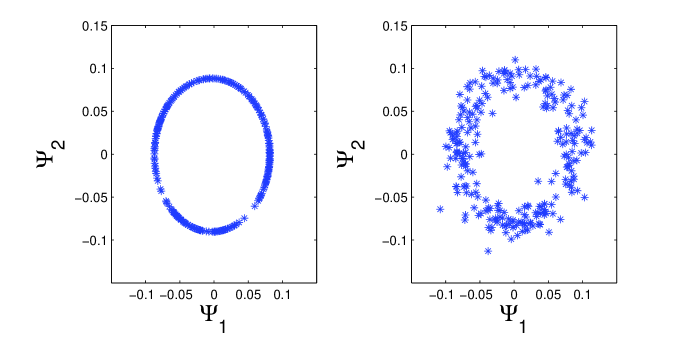
Figure 17: The two diffusion map coordinates (the first two nontrivial eigenvectors of $\mathbf{K}$) obtained from aligned, but noisy, MTW snapshots (right) and aligned, noise-free MTW snapshots (left).

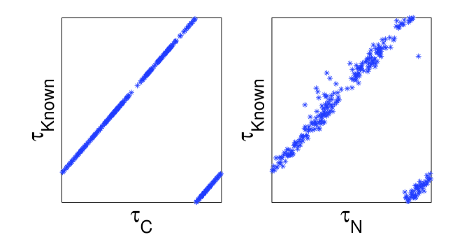
Figure 18: Parametrizations of the modulations via diffusion maps. On the $x$ axes, $\tau_{C}$ and $\tau_{N}$ (“clean” and ”noisy,” respectively), are computed from the diffusion map eigenvector information in Figure 17. On the $y$ axes, $\tau_{Known}$ is the “correct” parametrization. The plot of $\tau_{Known}$ vs. $\tau_{C}$ is shown just for comparison, for $\tau_{C}$ and $\tau_{Known}$ differ by only a phase offset. The two figures are roughly one-to-one (modulo $2\pi$).

7 Vector diffusion maps

In the preceding sections, we were able to take advantage of the eigenvector alignment method to provide information about the global alignment of ensembles of snapshots in two illustrative pattern-forming systems with symmetry. In the case of the orientational probability distributions of nematic liquid crystals (Section 4), all $M$ snapshots were in principle rotated versions of the same distribution function; due to the finiteness of the representation, however (each was a collection of $N$ representative particles), noise became a feature of the problem. For the spatiotemporally varying wave snapshots of the Kuramoto-Sivashinksy equation (Section 5), we were able to apply the eigenvector method to factor out the traveling component of the variation, even though each snapshot was not exactly the same up to rotation. We were successful because the modulation (superposed to the traveling component of the evolution) was relatively small. We then applied diffusion maps to the aligned snapshots and successfully recovered a meaningful, low-dimensional representation of the residual dynamics (the modulation).

Now, suppose that in the case of the LCP orientational probability distributions, the set of $M$ snapshots contained not only rotated realizations of the same (noisy) distribution, but also randomly rotated versions of snapshots that had evolved for different lengths of time. The differences in the $M$ snapshots would then be due to

• different finite particle realizations of the distribution function (only in the case $N\rightarrow\infty$ do they become the same);

• different rotations of these distribution function realizations; and

• the fact that the distribution function changes with time.

In such a situation, it might not be prudent to try to align two orientational probability distribution functions of vastly different shapes (these may arise from evolution over appreciably different lengths of time). A similar situation might arise if the modulation in our traveling/modulating wave snapshots is not small: pairwise alignments of vastly different shapes would stop being meaningful. Vector Diffusion Maps (Singer & Wu ) provide an approach that, in such circumstances, both help obtain global alignments and also reveal the underlying “symmetry-adjusted” reduced dynamics all in one step.

7.1 A brief introduction to vector diffusion maps

The reduced descriptions of the dynamics obtained by diffusion maps (as we did in the KSE example above) rely on the user’s ability to provide a pairwise similarity measure $\mathbf{W}_{ij}$ between snapshots $i$ and $j$. From there, the largest eigenvalues (and corresponding eigenvectors) of a matrix $\mathbf{K}$ are computed, where $\mathbf{K}_{ij}=\mathbf{W}_{ij}/\sum_{k}\mathbf{W}_{ik}$. In the case of the KSE wave snapshots, we set

$$\mathbf{W}_{ij}=\mbox{exp}\left[\frac{\sum_{k=1}^{128}\left[u(x_{k},t_{i})-u(x_{k},t_{j})\right]^{2}}{\varepsilon}\right]$$ (36)

(see Section 6). Intuitively, the eigenvectors of $\mathbf{K}$ corresponding to the largest eigenvalues are those related to the most robust diffusions in a graph whose vertices are the data (see, e.g. Belkin & Niyogi (2003)); if snapshot $i$ is “close” to snapshot $j$ in diffusion map space, then it should be possible to transition from the one to the other easily through mutually neighboring snapshots $k$, neighbors of neighbors, etc.

Likewise, the global alignments provided by the eigenvector method rely on the user to first compare all snapshots in a pairwise fashion so as to obtain the group element $g_{ij}\in G$ which “best” aligns them, and then incorporate the real/complex representation of this group element, $\mathbf{O}_{ij}$, into the $ij$-th block of a matrix. In the case of the KSE wave snapshots, we denoted this group element $\mathbf{O}_{ij}$ as

$$\mathbf{T}_{ij}=\mbox{exp}(-2i\pi a_{ij}/128)$$ (37)

(see Section 3). Intuitively, the eigenvector of $\mathbf{O}$ with largest corresponding eigenvalue corresponds to the most consistent global alignment; if snapshot $i$ can be rotated to snapshot $j$ via $g_{ij}$, then snapshot $i$ should also be able to be rotated to snapshot $j$ through a snapshot $k$ (via $g_{ik}g_{kj}$).

Vector diffusion maps attempts, in a sense, to combine the two methods (the eigenvector method and diffusion maps). To use vector diffusion maps, one first optimally aligns two snapshots $i$ and $j$ to obtain $g_{ij}$ and thus $\mathbf{O}_{ij}$; one then computes the similarity of $i$ and $j$ after this alignment has taken place to obtain $\mathbf{W}_{ij}$ (and, after normalization, $\mathbf{K}_{ij}$). A matrix $\mathbf{S}$ is then formed whose $ij$-th block is simply $\mathbf{S}_{ij}=\mathbf{K}_{ij}\mathbf{O}_{ij}$. The eigenvectors of $\mathbf{S}$ corresponding to its largest eigenvalues are computed, and these eigenvectors provide information about both symmetry adjustment (“alignment”) and about dynamic similarity. Distances between snapshots in this new vector diffusion map space are called vector diffusion distances (see equations (4.2) and (4.6) on p. 11 of Singer & Wu ). As we noted above, alignment comparisons between snapshots should only be trusted when $\mathbf{W}_{ij}$ is not small, for it may not make sense to compare two snapshots which differ appreciably (e.g. in shape and/or in temporal evolution time ). Vector diffusion maps accomplishes this by effectively ignoring comparisons $\mathbf{O}_{ij}$ for snapshots which are “far away” (small $\mathbf{W}_{ij}$) from each other.

7.2 Application of vector diffusion maps to the spatiotemporal wave snapshots of the KSE

To apply vector diffusion maps to the KSE example, we form the matrix $\mathbf{S}$ by setting

$$\mathbf{S}_{ij}=\mathbf{T}_{ij}\mathbf{K}_{ij},$$ (38)

where the the $\mathbf{T}_{ij}$ are obtained by optimally aligning each pair of noisy wave snapshots, and the $\mathbf{K}_{ij}$ are then computed on the symmetry-adjusted wave snapshots (these $\mathbf{K}_{ij}$ are, as before, $\mathbf{W}_{ij}/\sum_{k}\mathbf{W}_{ik}$).

The top eigenvectors of $\mathbf{S}$ are then computed, and the eigenvalues are exactly as in Section 6: $1.00,\,0.90,\,0.87,\,0.62,\,0.43,\,\ldots$ This is not surprising, for this particular problem actually “decouples”; the modulation is independent of the traveling motion for an exact modulated traveling wave (in other, more general problems, this is unlikely to be the case). The first eigenvector $\mathbf{v}_{0}$, the one corresponding to eigenvalue $1.00$, reveals the global alignments (see Section 5.5) and has the form

$$\mathbf{v}_{0}=\left[\begin{array}[]{c}\mbox{exp}(2i\pi a_{1}/128)\\ \mbox{exp}(2i\pi a_{2}/128)\\ \vdots\\ \mbox{exp}(2i\pi a_{M}/128)\end{array}\right].$$ (39)

The next two eigenvectors reveal the diffusion map parametrization of the underlying, symmetry-adjusted dynamics (the modulation, see Section 6). These eigenvectors are “corrupted” because they also contain the global alignments:

$$\mathbf{v}_{1,2}=\left[\begin{array}[]{c}\mbox{exp}(2i\pi a_{1}/128)\vec{\psi}_{1,2}^{(1)}\\ \mbox{exp}(2i\pi a_{2}/128)\vec{\psi}_{1,2}^{(2)}\\ \vdots\\ \mbox{exp}(2i\pi a_{M}/128)\vec{\psi}_{1,2}^{(M)}\end{array}\right].$$ (40)

However, one can easily get $\mathbf{v}_{1}$ and $\mathbf{v}_{2}$ back to their more meaningful, “original” forms $\vec{\psi}_{1}$ and $\vec{\psi}_{2}$ of Section 6 by simply dividing each of them entrywise by $\mathbf{v}$.

Since this particular example “decouples,” the global alignments and eigenvectors obtained this way agree with those already computed and shown in Figures 14 and 17; we do not plot them again here.

8 Summary and conclusions

In this paper we applied both the “eigenvector method” (Singer (2011); Singer et al. ; Singer & Shkolnisky ), and vector diffusion maps (Singer & Wu ) (based on the eigenvector method) to adjust data ensembles (consisting of snapshots from two evolving systems) with respect to the system intrinsic symmetries. We demonstrated the ability of both vector diffusion maps and the eigenvector method to align (and in a sense, denoise) the data sets, and also parameterize their symmetry-adjusted dynamics. For both examples, the eigenvector method provided a global alignment of the noisy snapshots of the evolving systems, even with a small signal-to-noise ratio. Additionally, for the case of traveling and modulating waves, vector diffusion maps were shown to both remove the underlying symmetry and capture the underlying long-term dynamics (the residual dynamics of modulation, after the “traveling” symmetry has been removed).

The two techniques are fast and easy to implement, and as discussed, they are a natural analogue to diffusion maps (Coifman & Lafon (2006)) in the sense that they rely on pairwise comparison data. This information is incorporated into an eigenvalue problem, whose result is a globally consistent (in a certain sense, see Section 3) parametrization/alignment of the underlying data set. Just as diffusion maps are robust to noise in the computation of the pairwise similarity measurements, vector diffusion maps and the eigenvector method are robust to both noise and alignment error in the computation of both the pairwise similarity measurements and symmetry group members.

By taking into account the equivariance of the system dynamics with respect to the underlying symmetry, vector diffusion maps may reduce the amount of data required in order to successfully elucidate an effective, low-dimensional description of the dynamics. Despite the success of nonlinear dimensionality reduction techniques in finding meaningful reduced descriptions for complex systems (see, e.g. Erban et al. (2007); Sonday et al. (2009); Das et al. (2006)), they still suffer from the curse of dimensionality; in general, the amount of data required to successfully recover $d$ “intrinsic” dimensions grows exponentially with $d$. Factoring out dimensions associated with the symmetry degrees of freedom will partially alleviate of this problem. While diffusion maps treats the snapshots as living on a manifold $\mathcal{M}$, vector diffusion maps in effect treats the snapshots as if they live in the quotient space $\mathcal{M}/G$. This implicit reduction of dimensionality allows the methods presented in this paper to provide an improved organization of the data.

9 Acknowledgments

B.E.S. was partially supported by the DOE CSGF (grant number DE-FG02-97ER25308) and the NSF GRFP. A.S. and I.G.K. were partially supported by the DOE (grant numbers DE-SC0002097 and DE-SC0005176), and A.S. also thanks the Sloan research fellowship. The authors would also like to acknowledge Constantinos I. Siettos for generously providing the LCP codes used in Section 4.

blah
Appendix: initialization of a probability distribution with the Metropolis-Hastings algorithm

To initialize $N$ particles $\{\mathbf{w}_{i}\}_{i=1}^{N}$ on the unit sphere consistently with some $\psi(\mathbf{u})$, we use the Metropolis-Hastings algorithm (Metropolis et al. (1953)). This algorithm may be used to design a Markov chain with stationary distribution equal to the desired $\psi(\mathbf{u})$. After an initial “relaxation” period of a few iterations, consecutive states $\mathbf{w}_{k}$ of the chain are statistically equivalent to samples drawn from $\psi(\mathbf{u})$.

An auxiliary distribution $q(\bullet|\mathbf{u})$, for example, a multivariate normal distribution with some mean vector and covariance matrix, is first selected. This $q$ distribution is used to generate, from the current state $\mathbf{w}_{k}$, a potential next state $\mathbf{w}_{cand}$. $q$ may be tuned carefully to reduce the variance in the empirically observed stationary distribution of the Markov chain; for our purposes, we choose to keep things simple and use $q=1$, meaning that at each step, we randomly generate a point $\mathbf{w}_{cand}$ on the unit sphere with no regard to the point $\mathbf{w}_{k}$ from which it originated. A candidate state $\mathbf{w}_{cand}$ generated by the auxiliary distribution is accepted with probability

$$p(\mathbf{w}_{k},\mathbf{w}_{cand})=\min\left[1,\frac{\psi(\mathbf{w}_{cand})q(\mathbf{w}_{k}|\mathbf{w}_{cand})}{\psi(\mathbf{w}_{k})q(\mathbf{w}_{cand}|\mathbf{w}_{k})}\right].$$ (41)

If the candidate $\mathbf{w}_{cand}$ is accepted, the next state becomes $\mathbf{w}_{k+1}=\mathbf{w}_{cand}$, otherwise if $\mathbf{w}_{cand}$ is rejected, the next state remains the same as the current state $\mathbf{w}_{k+1}=\mathbf{w}_{k}$. After running the Metropolis-Hastings algorithm for a large number of iterations, we subsample the Markov chain to reduce it to $N$ particles $\{\mathbf{w}_{i}\}_{i=1}^{N}$ on the unit sphere. These $N$ particles become our consistent initialization according to $\psi(\mathbf{u})$.

References

- Ahuja et al. (2007) Ahuja, S., Kevrekidis, I. G., & Rowley, C. W. (2007). Template-based stabilization of relative equilibria in systems with continuous symmetry. Journal of Nonlinear Science, 17, 109–143.
- Arecchi et al. (1999) Arecchi, F. T., Boccaletti, S., & Ramazza, P. L. (1999). Pattern formation and competition in nonlinear optics. Physics Reports, 318, 1–83.
- Aubry et al. (1993) Aubry, N., Lian, W., & Titi, E. (1993). Preserving symmetries in the proper orthogonal decomposition. SIAM Journal on Scientific Computing, 14, 483.
- Belkin & Niyogi (2003) Belkin, M., & Niyogi, P. (2003). Laplacian eigenmaps for dimensionality reduction and data representation. Neural computation, 15, 1373–1396.
- Berkooz et al. (1993) Berkooz, G., Holmes, P., & Lumley, J. L. (1993). The proper orthogonal decomposition in the analysis of turbulent flows. Annual Review of Fluid Mechanics, 25, 539–575.
- Berkooz & Titi (1993) Berkooz, G., & Titi, E. S. (1993). Galerkin projections and the proper orthogonal decomposition for equivariant equations. Physics Letters A, 174, 94–102.
- (7) Cheng, X., & Singer, A. (). The Spectrum of an Hermitian Matrix With Dependent Entries Constructed from Random Independent Images. in preparation, .
- Coifman et al. (2005a) Coifman, R., Lafon, S., Lee, A., Maggioni, M., Nadler, B., Warner, F., & Zucker, S. (2005a). Geometric diffusions as a tool for harmonic analysis and structure definition of data: Diffusion maps. PNAS, 102, 7426.
- Coifman et al. (2005b) Coifman, R., Lafon, S., Lee, A., Maggioni, M., Nadler, B., Warner, F., & Zucker, S. (2005b). Geometric diffusions as a tool for harmonic analysis and structure definition of data: Multiscale methods. PNAS, 102, 7432.
- Coifman & Lafon (2006) Coifman, R. R., & Lafon, S. (2006). Diffusion maps. Applied and Computational Harmonic Analysis, 21, 5–30.
- Constantin et al. (1988) Constantin, P., Foias, C., Nicolaenko, B., & Temam, R. (1988). Integral manifolds and inertial manifolds for dissipative partial differential equations. “Applied Mathematical Science Series,” No. 70, Springer-Verlag, New York.
- Cross & Hohenberg (1993) Cross, M. C., & Hohenberg, P. C. (1993). Pattern formation outside of equilibrium. Reviews of Modern Physics, 65, 851–1112.
- Das et al. (2006) Das, P., Moll, M., Stamati, H., Kavraki, L., & Clementi, C. (2006). Low-dimensional, free-energy landscapes of protein-folding reactions by nonlinear dimensionality reduction. PNAS, 103, 9885.
- Erban et al. (2007) Erban, R., Frewen, T. A., Wang, X., Elston, T. C., Coifman, R., Nadler, B., & Kevrekidis, I. G. (2007). Variable-free exploration of stochastic models: a gene regulatory network example. The Journal of chemical physics, 126, 155103.
- Fan & Hoffman (1955) Fan, K., & Hoffman, A. J. (1955). Some metric inequalities in the space of matrices. Proceedings of the American Mathematical Society, 6, 111–116.
- Féral & Péché (2007) Féral, D., & Péché, S. (2007). The largest eigenvalue of rank one deformation of large Wigner matrices. Communications in Mathematical Physics, 272, 185–228.
- Foias et al. (1988a) Foias, C., Jolly, M. S., Kevrekidis, I. G., Sell, G. R., & Titi, E. S. (1988a). On the computation of inertial manifolds. Physics Letters A, 131, 433–436.
- Foias et al. (1988b) Foias, C., Sell, G. R., & Temam, R. (1988b). Inertial manifolds for nonlinear evolutionary equations. Journal of Differential Equations, 73, 309–353.
- Foias et al. (1989) Foias, C., Sell, G. R., & Titi, E. S. (1989). Exponential tracking and approximation of inertial manifolds for dissipative nonlinear equations. Journal of Dynamics and Differential Equations, 1, 199–244.
- Grassberger & Procaccia (1983) Grassberger, P., & Procaccia, I. (1983). Measuring the strangeness of strange attractors. Physica D: Nonlinear Phenomena, 9, 189–208.
- Guckenheimer & Holmes (2002) Guckenheimer, J., & Holmes, P. (2002). Nonlinear oscillations, dynamical systems, and bifurcations of vector fields. Springer.
- Holmes et al. (1998) Holmes, P., Lumley, J. L., & Berkooz, G. (1998). Turbulence, coherent structures, dynamical systems and symmetry. Cambridge Univ Pr.
- Jolly (1989) Jolly, M. S. (1989). Explicit construction of an inertial manifold for a reaction diffusion equation. Journal of Differential Equations, 78, 220–261.
- Jolly et al. (1990) Jolly, M. S., Kevrekidis, I. G., & Titi, E. S. (1990). Approximate inertial manifolds for the Kuramoto-Sivashinsky equation: analysis and computations. Physica D, 44, 38–60.
- Keller (1975) Keller, J. B. (1975). Closest unitary, orthogonal and hermitian operators to a given operator. Mathematics Magazine, 48, 192–197.
- Kevrekidis et al. (2008) Kevrekidis, P. G., Frantzeskakis, D. J., & Carretero-González, R. (2008). Emergent nonlinear phenomena in Bose-Einstein condensates. Theory and experiment, .
- Kunisch & Volkwein (2003) Kunisch, K., & Volkwein, S. (2003). Galerkin proper orthogonal decomposition methods for a general equation in fluid dynamics. SIAM Journal on Numerical Analysis, (pp. 492–515).
- Kuramoto & Tsuzuki (1976) Kuramoto, Y., & Tsuzuki, T. (1976). Persistent propagation of concentration waves in dissipative media far from thermal equilibrium. Prog. Theor. Phys, 55, 356–369.
- Lafon & Lee (2006) Lafon, S., & Lee, A. B. (2006). Diffusion maps and coarse-graining: a unified framework for dimensionality reduction, graph partitioning, and data set parameterization. Pattern Analysis and Machine Intelligence, IEEE Transactions on, 28, 1393.
-
Maier & Saupe (1959)
Maier, W., & Saupe, A.
(1959).
Eine einfache molekularstatistische Theorie der
nematischen kristallinfl
”ussigen Phase. Teil I. Zeitschrift Naturforschung Teil A, 14, 882. - Metropolis et al. (1953) Metropolis, N., Rosenbluth, A. W., Rosenbluth, M. N., Teller, A. H., & Teller, E. (1953). Equation of state calculations by fast computing machines. The journal of chemical physics, 21, 1087.
- Nadler et al. (2006) Nadler, B., Lafon, S., Coifman, R., & Kevrekidis, I. G. (2006). Diffusion maps, spectral clustering and eigenfunctions of fokker-planck operators. Advances in Neural Information Processing Systems, 18, 955.
- Neumaier (2001) Neumaier, A. (2001). Generalized Lyapunov-Schmidt reduction for parametrized equations at near singular points. Linear Algebra and its Applications, 324, 119–131.
- Papoulis (1977) Papoulis, A. (1977). Signal analysis. McGraw-Hill New York.
- Rokhlin & Tygert (2006) Rokhlin, V., & Tygert, M. (2006). Fast Algorithms for Spherical Harmonic Expansions. SIAM Journal on Scientific Computing, 27, 1903.
- Roweis & Saul (2000) Roweis, S. T., & Saul, L. K. (2000). Nonlinear dimensionality reduction by locally linear embedding. Science, 290, 2323.
- Rowley & Marsden (2000) Rowley, C. W., & Marsden, J. E. (2000). Reconstruction equations and the Karhunen-Loeve expansion for systems with symmetry. Physica D: Nonlinear Phenomena, 142, 1–19.
- Siettos et al. (2003) Siettos, C. I., Graham, M. D., & Kevrekidis, I. G. (2003). Coarse Brownian dynamics for nematic liquid crystals: Bifurcation, projective integration, and control via stochastic simulation. The Journal of Chemical Physics, 118, 10149.
- Singer (2011) Singer, A. (2011). Angular Synchronization by Eigenvectors and Semidefinite Programming. Applied and Computational Harmonic Analysis, 30, 20–36.
- (40) Singer, A., & Shkolnisky, Y. (). Three-Dimensional Structure Determination from Common Lines in Cryo-EM by Eigenvectors and Semidefinite Programming. accepted by SIAM Journal on Imaging Sciences, .
- (41) Singer, A., & Wu, H. T. (). Vector Diffusion Maps and the Connection Laplacian.
- (42) Singer, A., Zhao, Z., Shkolnisky, Y., & Hadani, R. (). Viewing Angle Classification of Cryo-Electron Microscopy Images using Eigenvectors. submitted, .
- Sirisup et al. (2005) Sirisup, S., Karniadakis, G. E., Xiu, D., & Kevrekidis, I. G. (2005). Equation-free/Galerkin-free POD-assisted computation of incompressible flows. Journal of Computational Physics, 207, 568–587.
- Sirovich (1987) Sirovich, L. (1987). Turbulence and the dynamics of coherent structures. I-III. Quarterly of applied mathematics, 45, 561–571.
- Sivashinsky (1977) Sivashinsky, G. I. (1977). Nonlinear analysis of hydrodynamic instability in laminar flames–I. Derivation of basic equations. Acta Astronautica, 4, 1177–1206.
- Sonday et al. (2009) Sonday, B. E., Haataja, M., & Kevrekidis, I. G. (2009). Coarse-graining the dynamics of a driven interface in the presence of mobile impurities: Effective description via diffusion maps. Physical Review E, 80, 31102.
- Tenenbaum et al. (2000) Tenenbaum, J. B., Silva, V., & Langford, J. C. (2000). A global geometric framework for nonlinear dimensionality reduction. Science, 290, 2319.
- Titi (1990) Titi, E. S. (1990). On approximate inertial manifolds to the Navier-Stokes equations. Journal of mathematical analysis and applications, 149, 540–557.