Abstract

In the pedestal of a tokamak, the sharp radial gradients of density and temperature can give rise to poloidal variation in the density of impurities. At the same time, the flow of the impurity species is modified relative to the conventional neoclassical result. In this paper, these changes to the density and flow of a collisional impurity species are calculated for the case when the main ions are in the plateau regime. In this regime it is found that the impurity density can be higher at either the inboard or outboard side. This finding differs from earlier results for banana- or Pfirsch-Schlüter-regime main ions, in which case the impurity density is always higher at the inboard side in the absence of rotation. Finally, the modifications to the impurity flow are also given for the other regimes of main-ion collisionality.

I Introduction

Conventional theory of neoclassical transport in tokamaks HH ; HS is not applicable to regions where the pressure and temperature profiles are very steep, such as the pedestal at the plasma edge. As the radial scale length decreases, poloidal variation arises in the temperature and density of each species. In an impure plasma, typically the first quantity to develop a poloidal variation is the impurity density, and indeed, strong poloidal impurity asymmetries have been observed in experiments marr ; newcmod . In Refs. perbif ; fh1 ; fh2 , neoclassical theory for an impure plasma was extended to allow for larger gradients than are usually considered. Specifically, the gradients were allowed to be so large that the friction between the bulk ions and heavy impurity ions could compete with the parallel impurity pressure gradient, as is typically the case in the tokamak edge. Mathematically, this means that the parameter $\Delta\equiv\delta\hat{\nu}_{ii}z^{2}$ was assumed to be of order unity, but the poloidal Larmor radius of the bulk ions divided by the radial scale length associated with the density and temperature profiles $\delta=\rho_{\theta}/L_{\perp}$ was assumed to be small. Here $z$ is the impurity charge number, $\hat{\nu}_{ii}=L_{\parallel}/\lambda_{i}$ is a measure of the ion collisionality, $\lambda_{i}$ is the bulk ion mean-free path, and $L_{\parallel}$ is the connection length. It was shown that the impurity dynamics then become nonlinear, and if the pressure and temperature gradients of the main ion species are sufficiently steep, the impurities are pushed to the inboard side of the flux surface.

Recently, the in-out density asymmetry $A=n_{H}/n_{L}$ was measured for boron impurities in Alcator C-Mod  marr . Here, $n_{H}$ and $n_{L}$ refer respectively to the impurity density at the high-field-side midplane and low-field-side midplane of a given flux surface. It was observed that $A$ could be either less than or greater than one. A comparison was made to a theoretical model of impurity asymmetry in strong gradient regions fh2 in which the primary ion species was assumed to be in the Pfirsch-Schlüter regime of collisionality. This model predicts that $A$ must be more than one, and for the parameters of the Alcator C-Mod experiments, the predicted $A$ was systematically closer to unity than the measured ratio. One factor which likely contributes to the discrepancy is that much of the data were taken in a region in which the main ions were in the plateau collisionality regime rather than the Pfirsch-Schlüter regime. Reference marr therefore suggests that an analogous theoretical model should be developed for the plateau regime, and it is the purpose of this paper to present such a model. Impurity asymmetry in the banana collisionality regime has been analyzed previously in perbif ; fh1 . Other than the collisionality, the present work uses the same orderings as the previous models: $\Delta\sim 1,z\gg 1,$ and $\delta\ll 1$.

The poloidal rearrangement of the impurities affects the impurity velocity due to the requirement of mass conservation. In previous work on the banana and Pfirsch-Schlüter regimes, this alteration to the impurity flow was not explicitly calculated. However, pedestal impurity flows are measured routinely in experiments  marr ; newcmod , so impurity flows represent an important point of comparison between experiment and theory. The measurements and conventional neoclassical theory often disagree. In particular, when the main ions are in the plateau or banana collisionality regime, the measured impurity flow is greater in the direction of the electron diamagnetic velocity than predicted. Consequently, in this paper we give explicit forms for the modified impurity flows, and we examine whether the modifications are sufficient to reconcile neoclassical theory with the experimental measurements.

The remainder of the paper is organized as follows. In Sec. II we describe the kinetics of main ions in the plateau regime. In Sec. III we analyze the parallel momentum equation for the impurities and derive an equation that governs their poloidal rearrangement. We show approximate solutions in several limits and numerical solutions are also presented. In Sec. IV we explore the modification of the poloidal impurity rotation due to the presence of large gradients, discussing all regimes of main-ion collisionality. Finally, the results are summarized and discussed in Sec. V.

II Kinetics of main ions in the plateau regime

The plasma is assumed to consist of hydrogenic ions ($i$) in the plateau regime, collisional (Pfirsch-Schlüter) impurities ($z$), and electrons ($e$). The calculation does not depend on the collisionality regime of the electrons. The magnetic field is represented as $\mbox{\boldmath$B$}=I(\psi)\nabla\varphi+\nabla\varphi\times\nabla\psi$, where $\varphi$ is the toroidal angle and $2\pi\psi$ is the poloidal flux. Throughout this analysis we will use a poloidal angle coordinate $\vartheta$ which is chosen so that $\mbox{\boldmath$B$}\cdot\nabla\vartheta$ is a flux function. This coordinate makes flux surface averages convenient to evaluate ($\left\langle Y\right\rangle=(2\pi)^{-1}\int_{0}^{2\pi}Yd\vartheta$ for any quantity $Y$), and this coordinate is equivalent to the $\vartheta$ used in perbif ; fh1 ; fh2 . We assume a model field magnitude $b^{2}=1-2\epsilon\cos\vartheta$ where $b=B/\left\langle B^{2}\right\rangle^{1/2}$ and $\epsilon=r/R$ is the inverse aspect ratio. We must assume $\epsilon\ll 1$ from the beginning of the analysis in order for a plateau regime to exist.

The gyroaveraged ion distribution function in the plateau regime is then given by pusztai $\bar{f}_{i}=f_{Mi}+\bar{f}_{i1}$ where

$$f_{Mi}=n_{i0}(\psi)\left(\frac{m_{i}}{2\pi T_{i}(\psi)}\right)^{3/2}\exp\left(-\frac{m_{i}v^{2}}{2T_{i}(\psi)}\right)$$ (1)

is a stationary Maxwellian and a flux function,

$$\bar{f}_{i1}=-f_{Mi}\frac{e\Phi_{1}}{T_{i}}+H_{i}-f_{Mi}v_{\|}\frac{I}{\Omega_{i}}\left(\frac{p_{i}^{\prime}}{p_{i}}+\frac{e\Phi_{0}^{\prime}}{T_{i}}+\frac{yb^{2}T_{i}^{\prime}}{2T_{i}}\right),$$ (2)

$p_{i}=n_{i0}T_{i}$, $\Omega_{i}=eB/m_{i}$ is the ion cyclotron frequency, primes denote $d/d\psi$, $\Phi_{0}=\left\langle\Phi\right\rangle$, $\Phi_{1}=\Phi-\Phi_{0}$,

$$H_{i}=Q_{i}\frac{\hat{\nu}_{i}\sin\vartheta-x_{\|}\cos\vartheta}{x_{\|}^{2}+\hat{\nu}_{i}^{2}}\approx Q_{i}\left[\pi\delta(x_{\|})\sin\vartheta-\frac{\cos\vartheta}{x_{\|}}\right],$$ (3)

$\hat{\nu}_{i}=\nu_{i}qR/v_{i}$ is the normalized collisionality, $x=v/v_{i}$, $v_{i}=(2T_{i}/m_{i})^{1/2}$,

$$Q_{i}=f_{Mi}\frac{\epsilon v_{i}IT_{i}^{\prime}}{4\Omega_{i}T_{i}}\left[(2x_{\|}^{2}+x_{\perp}^{2})(2x^{2}-5)+yb^{2}(2x_{\|}^{2}-x_{\perp}^{2})\right],$$ (4)

and $y$ is a velocity-independent coefficient which will be determined by the requirement of ambipolarity. In a pure plasma this requirement leads to $y=1$, but the presence of impurities will alter the value. Also, $y$ must be a flux function so that $\nabla\cdot(n_{i}\mbox{\boldmath$V$}_{i})=0$.

III Impurity dynamics

The parallel momentum equation for the impurities is taken to be

$$0=-zn_{z}e\nabla_{\parallel}\Phi-T_{i}\nabla_{\parallel}n_{z}+R_{zi\parallel}$$ (5)

where $R_{zi\parallel}$ is the impurity-ion friction. The parallel viscosity of the impurities has been neglected since it was shown in Ref perbif to be smaller than the pressure gradient if $\delta/z\hat{\nu}_{ii}\ll 1$, which is usually the case in the tokamak edge. As also shown in that paper, the impurity temperature is then equilibrated with the bulk ion temperature and is therefore constant over the flux surface. The poloidal electric field $-\nabla_{||}\Phi$ can be obtained from the quasi-neutrality condition $zn_{z}=n_{e}-n_{i}$ using $n_{e}=(1+e\Phi_{1}/T_{e})n_{e0}(\psi)$ and using the distribution function (2) to calculate the ion density:

$$n_{i}=n_{i0}\left(1-\frac{e\Phi_{1}}{T_{i}}+\epsilon N_{s}\sin{\vartheta}\right),$$ (6)

where

$$N_{s}=-\frac{\sqrt{\pi}v_{i}IT_{i}^{\prime}}{4\Omega_{i}T_{i}}\left(1+b^{2}y\right).$$ (7)

The result is

$$\frac{ze\nabla_{\parallel}\Phi}{T_{i}}=\frac{T_{0}}{2T_{i}n_{0}}\nabla_{\parallel}\left(z^{2}n_{z}+zn_{i0}\epsilon N_{s}\sin{\vartheta}\right),$$ (8)

where $2n_{0}/T_{0}\equiv n_{e0}/T_{e}+n_{i0}/T_{i}$. Equation (5) then becomes

$$(1+\alpha n)\nabla_{\parallel}n+\frac{\epsilon zT_{0}n_{i0}n}{2T_{i}n_{0}}\nabla_{\parallel}\left(N_{s}\sin{\vartheta}\right)=\frac{R_{zi\parallel}}{\langle n_{z}\rangle T_{i}}$$ (9)

where $n=n_{z}/\langle n_{z}\rangle$ is the normalized impurity density and $\alpha\equiv\left\langle n_{z}\right\rangle z^{2}T_{0}/(2n_{0}T_{i})$. In the rest of the analysis we will order $\alpha\sim 1$, which is equivalent (for $T_{e}\sim T_{i}$) to the ordering $z_{eff}-1\sim 1$.

Next, the ion-impurity collision operator $C_{iz}$ is inserted in $R_{zi\parallel}=-m_{i}\int d^{3}v\,v_{||}C_{iz}$ to write

$$R_{zi\parallel}=-\int d^{3}v\,m_{i}v_{\parallel}\nu_{iz}\left({\cal L}(f_{i}-f_{i0})+\frac{m_{i}v_{\parallel}}{T_{i}}V_{z\parallel}f_{i0}\right)$$ (10)

where

$${\cal L}=\frac{2v_{\parallel}}{v^{2}B}\frac{\partial}{\partial\lambda}\lambda v_{\parallel}\frac{\partial}{\partial\lambda}$$ (11)

is the Lorentz pitch-angle scattering operator, $\lambda=v_{\perp}^{2}/(Bv^{2})$, $\nu_{iz}=3\pi^{1/2}/(4\tau_{iz}x^{3})$, and $\tau_{iz}=3(2\pi T_{i})^{3/2}\epsilon_{0}^{2}m_{i}^{1/2}/(n_{z}z^{2}e^{4})$ is the ion-impurity collision time. To ensure $\nabla\cdot(n_{z}\mbox{\boldmath$V$}_{z})=0$, the parallel impurity flow velocity must have the form perbif

$$V_{z\parallel}=-\frac{I\Phi_{0}^{\prime}}{B}+\frac{K_{z}(\psi)B}{n_{z}}$$ (12)

where $K_{z}(\psi)$ is proportional to the poloidal velocity. Using the main-ion distribution function (2) we then obtain

$$R_{zi\parallel}=-\frac{I}{\Omega_{i}\tau_{iz}}\left(p_{i}^{\prime}+\frac{yb^{2}n_{i0}T_{i}^{\prime}}{2}\right)-\frac{m_{i}n_{i0}K_{z}B}{\tau_{iz}n_{z}}+Q_{r},$$ (13)

where

$$Q_{r}=m_{i}\int d^{3}v\nu_{iz}v_{\parallel}Q_{i}\left[\pi\delta(x_{\parallel})\sin{\vartheta}-\frac{x_{\parallel}}{x_{\parallel}^{2}+\hat{\nu}_{i}^{2}}\cos{\vartheta}\right].$$ (14)

For $\hat{\nu}_{i}\to 0$ the integration results in

$$Q_{r}=3\frac{\epsilon n_{i0}IT_{i}^{\prime}}{\tau_{iz}\Omega_{i}}\cos{\vartheta}.$$ (15)

To rewrite Eq. (9) in dimensionless form we introduce the ratio of the temperature and pressure scale lengths $\eta=p_{i}T_{i}^{\prime}/(T_{i}p_{i}^{\prime})$,

$$g=-\frac{m_{i}Ip_{i}^{\prime}}{eT_{i}\tau_{iz}n_{z}\mbox{\boldmath$B$}\cdot\nabla\vartheta},$$ (16)

and

$$\tau_{*}=\frac{\sqrt{\pi}zT_{0}\tau_{iz}n_{z}v_{i}\mbox{\boldmath$B$}\cdot\nabla\vartheta}{8T_{i}n_{0}B_{0}},$$ (17)

where $B_{0}=\left\langle B^{2}\right\rangle^{1/2}$. Notice that $g$, $\tau_{*}$, and $(\tau_{iz}n_{z})$ are $\vartheta$-independent, and the formal magnitude of $\tau_{*}\sim(z\hat{\nu}_{i})^{-1}$ has not yet been fixed. Equation (9) now becomes

$$(1+\alpha n)\frac{\partial n}{\partial\vartheta}=g\left\{n+\frac{\eta ynb^{2}}{2}-\epsilon\eta\left[3+(1+y)\tau_{*}\right]n\cos{\vartheta}+K_{z}\frac{n_{i0}eB^{2}}{\left\langle n_{z}\right\rangle Ip_{i}^{\prime}}\right\}$$ (18)

where we have used $\partial(N_{s}\sin\vartheta)/\partial\vartheta\approx\left\langle N_{s}\right\rangle\cos\vartheta$. (Other terms of order $\epsilon$ have already been discarded in deriving the distribution function (2).) Integrating Eq (18) over $\vartheta$ yields a solubility constraint which can be used to determine the poloidal impurity rotation,

$$K_{z}=\frac{\left\langle n_{z}\right\rangle Ip_{i}^{\prime}}{n_{i0}e\left\langle B^{2}\right\rangle}\left\{-1-\frac{\eta y}{2}\left\langle nb^{2}\right\rangle+\left[3+(1+y)\tau_{*}\right]\epsilon\eta\left\langle n\cos\vartheta\right\rangle\right\},$$ (19)

and Eq (18) becomes

$$(1+\alpha n)\frac{\partial n}{\partial\vartheta}=g\left[n-b^{2}+\frac{\eta yb^{2}}{2}\left(n-\left\langle nb^{2}\right\rangle\right)\right.\hskip 142.26378pt$$

$$\left.+\left[3+(1+y)\tau_{*}\right]\epsilon\eta\left(b^{2}\left\langle n\cos\vartheta\right\rangle-n\cos\vartheta\right)\right].$$ (20)

The $\cos\vartheta$ terms above can be significant despite being proportional to $\epsilon$, for the other drive in the equation is the $\vartheta$-variation in $b$, which is also $\mathcal{O}(\epsilon)$.

To make further progress we will calculate the coefficient $y$ by requiring ambipolarity. Due to the smallness of the electron mass, the ambipolarity condition is approximately $\Gamma_{i}=-z\Gamma_{z}$. As in the conventional plateau-regime calculation for a pure plasma, the main-ion flux is

$$\Gamma_{i}\equiv\langle\mbox{\boldmath$\Gamma$}_{i}\cdot\nabla\psi\rangle=\frac{\sqrt{\pi}\epsilon^{2}v_{i}^{3}I^{2}(\mbox{\boldmath$B$}\cdot\nabla\vartheta)n_{i0}T_{i}^{\prime}}{8\Omega_{i0}^{2}B_{0}T_{i}}(y-1)$$ (21)

where $\Omega_{i0}=eB_{0}/m_{i}$. The impurity flux is driven by the impurity-ion parallel friction force

$$\Gamma_{z}\equiv\left\langle\mbox{\boldmath$\Gamma$}_{z}\cdot\nabla\psi\right\rangle=\left\langle\frac{IR_{zi\parallel}}{zeB}\right\rangle,$$ (22)

where $R_{zi\parallel}$ is given by Eq. (13) with $K_{z}$ from (19). We find

$$\Gamma_{z}=\frac{m_{i}I^{2}\langle n_{z}\rangle p_{i}^{\prime}}{ze^{2}\tau_{iz}n_{z}\langle B^{2}\rangle}\left(1-\left\langle\frac{n}{b^{2}}\right\rangle+\frac{\eta y}{2}\left[\langle nb^{2}\rangle-1\right]\right.\hskip 142.26378pt$$

$$\left.+\epsilon\eta\left\{3\left\langle\frac{n\cos{\vartheta}}{b^{2}}\right\rangle-\left[3+(1+y)\tau_{*}\right]\left\langle n\cos{\vartheta}\right\rangle\right\}\right).$$ (23)

The condition for ambipolarity then gives

$$y=\frac{z\epsilon^{2}\tau_{*}\alpha^{-1}+\eta^{-1}(\left\langle n/b^{2}\right\rangle-1)-3\epsilon\left\langle nb^{-2}\cos\vartheta\right\rangle+(3+\tau_{*})\epsilon\left\langle n\cos\vartheta\right\rangle}{z\epsilon^{2}\tau_{*}\alpha^{-1}+2^{-1}(\left\langle nb^{2}\right\rangle-1)-\epsilon\tau_{*}\left\langle n\cos\vartheta\right\rangle}.$$ (24)

The pure plasma limit $y=1$ is recovered as $\alpha\to 0$.

The system (20) and (24) describes the poloidal rearrangement of the impurities. While (20) is similar to the equations found if the main ions are in the banana perbif ; fh1 or Pfirsch-Schlüter regimes fh2 , (20) has several different terms, and also the radial scale length entering $g$ is different (i.e. only the pressure scale length appears, rather than a combination of the pressure and temperature scale lengths.) As in Refs.perbif ; fh1 ; fh2 , $g$ measures the steepness of the bulk ion pressure profile. In conventional neoclassical theory $g$ is assumed to be small, which implies that the friction force is smaller than the parallel pressure gradient. We next examine how the integro-differential equation (20) can be solved analytically in a number of limits.

Weak density variation.

If $n-1\sim\mathcal{O}(\epsilon)$ then we can expand $n=1+n_{c}\cos{\vartheta}+n_{s}\sin{\vartheta}+O(\epsilon^{2})$ with $n_{s}$ and $n_{c}$ both $\sim\mathcal{O}(\epsilon)$. The solution of Eq (20) is then found to be

$$n_{s} = \epsilon g(1+\alpha)\frac{2-\eta[3+(1+y)\tau_{*}]}{(1+\alpha)^{2}+g^{2}(1+\eta y/2)^{2}},$$ (25)

$$n_{c} = -\epsilon g^{2}(1+\eta y/2)\frac{2-\eta[3+(1+y)\tau_{*}]}{(1+\alpha)^{2}+g^{2}(1+\eta y/2)^{2}}.$$ (26)

It can be noted from these expressions that as $p_{i}^{\prime}$ becomes larger, the impurities first develop an up-down asymmetry and then an in-out asymmetry. This same behaviour is found in the banana and Pfirsch-Schlüter regimes. However, in the plateau regime the asymmetry is proportional to the new factor $2-\eta[3+(1+y)\tau_{*}]$, which means that the sign of the asymmetry can be changed depending on the magnitude of $\eta$, $\tau_{*}$ and $y$. If $\eta>2/[3+(1+y)\tau_{*}]$, the impurities will be pushed to the outside of the flux surface. This result is different from the analogous $n-1\sim\mathcal{O}(\epsilon)\ll 1$ limits when the main ions are in the banana or Pfirsch-Schlüter regimes. In these cases, in the absence of rotation, the impurities were pushed to the inside, regardless of the ratio of the pressure and temperature gradients.

Large gradients.

In the $g\gg 1$ limit, corresponding to a large pressure gradient, we can expand (20) in $g^{-1}$. To lowest order, the right-hand side of (20) must vanish, giving $n\approx\tilde{n}/\left\langle\tilde{n}\right\rangle$ where

$$\tilde{n}=\frac{b^{2}}{1+(\eta y/2)b^{2}-\epsilon\eta[3+(1+y)\tau_{*}]\cos{\vartheta}}.$$ (27)

In this case there is only in-out asymmetry. Expanding in $\epsilon$ then gives

$$n=1+2\epsilon(S-1)\cos\vartheta$$ (28)

where $S=\eta\left[3+y+(1+y)\tau_{*}\right]/(2+\eta y)$. (This same result can also be obtained by a $g\gg 1$ expansion of (26).) The impurity density evidently may be higher at either the inboard side $(S<1)$ or outboard side $(S>1)$. This finding too differs from the corresponding $g\gg 1$ limits when the main ions are in the banana or Pfirsch-Schlüter regime. In these cases, the impurity density is always greater at the inboard side (even when there is significant rotation).

Numerical solution.

For $\alpha\ll 1$, equation (20) may be solved numerically with the following iterative procedure. A small number (5-10) of poloidal Fourier modes are considered. An initial guess for $n(\vartheta)$ is used to compute $y$ and the nonlinear term $\alpha n\;\partial n/\partial\vartheta$. An improved $n(\vartheta)$ is then calculated using (20), and the process is repeated until convergence is achieved. Typical results are shown in Figure 1. Figure 2 shows the in-out asymmetry factor

$$A=\frac{n(\vartheta=\pi)}{n(\vartheta=0)}$$ (29)

over a wide range of parameters.

Figure (3) shows the in-out asymmetry $A$ for $\epsilon=0.3$, $g=10$, and the trace impurity limit $y\to 1$. A nearly identical plot can be generated using the $g\gg 1$ expressions (27) or (28), although the precise value of $A$ in the $A<1$ region is somewhat different due to the fact that $\epsilon=0.3$ is not much smaller than one.

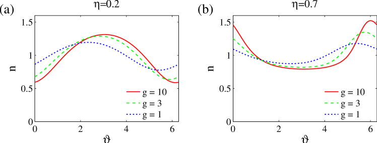
Figure 1: (Color online) Normalized impurity density as function of poloidal angle, calculated by numerical solution of (20) and (24). The parameters used are $\epsilon=0.3$, $\tau_{\ast}=0.5$, $z=5$, and $\alpha=0.25$. Other values of $\alpha$ from 0 to 1 produce nearly indistinguishable results.

Figure 2: (Color online) Contours of the in-out asymmetry $A$, decreasing monotonically with $\eta$, for (a) $\tau_{*}=0.1$ and (b) $\tau_{*}=1.0$. The other parameters are $\epsilon=0.3$, $z=5$, and $\alpha=0.25$. Results for $\alpha=0$ are nearly indistinguishable. Solid contours run from $A=3$ to 1 in steps of 0.5. Dashed contours decrease from $A=0.9$ to 0.6 (a) or 0.2 (b) in steps of 0.1.

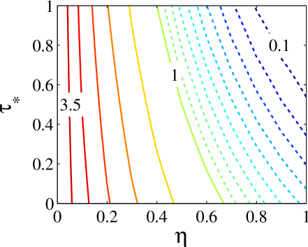
Figure 3: (Color online) Contours of the in-out asymmetry factor $A$ in the $g\gg 1$ and trace impurity ($y\to 1$) limit and with $\epsilon=0.3$. Solid contours range from 3.5 to 1 with spacing of 0.5, and dashed contours range from 0.9 to 0.1 with spacing of 0.1.

IV Poloidal impurity rotation

If the impurity density varies on a flux surface, the impurity poloidal rotation will be different from the one derived in conventional neoclassical theory. Using (12) and (19), we can write

$$V_{z\vartheta}^{pl}=\frac{B_{\vartheta}K_{z}}{n_{z}}=-X\frac{IB_{\vartheta}}{ne\left\langle B^{2}\right\rangle}\left[\frac{T_{i}}{n_{i0}}\frac{dn_{i0}}{d\psi}+\frac{3}{2}\frac{dT_{i}}{d\psi}\right],$$ (30)

where

$$X=\left(1+\frac{\eta}{2}\right)^{-1}\left\{1+\frac{\eta y}{2}\left\langle nb^{2}\right\rangle-\left[3+(1+y)\tau_{*}\right]\epsilon\eta\left\langle n\cos\vartheta\right\rangle\right\}$$ (31)

is constant on a flux surface. The definition of $X$ was chosen above so that in the trace impurity limit ($\alpha\to 0$, $y\to 1$) and if $n_{z}$ is also uniform on a flux surface (i.e. $g\to 0$), then $X\to 1$. This limit reproduces the conventional neoclassical result HS ; cattosimakov .

Figure 4 shows the scale factor $X$ for various values of $\eta$, $\tau_{*}$, and $g$. The figure was calculated using $\epsilon=0.3$ and $\alpha\to 0$. It is evident that when $g>1$, the poloidal flow can be significantly suppressed compared to the conventional neoclassical result if $\eta$ and $\tau_{*}$ approach one. The situation is only slightly different when the relative impurity strength $\alpha$ is nonzero, as shown in Figure 5. This figure is equivalent to Figure 4.a but with $\alpha$ raised to 0.25 and $z=5$. When $\tau_{*}\ll 1$, the flow now becomes slightly enhanced compared to the conventional neoclassical result.

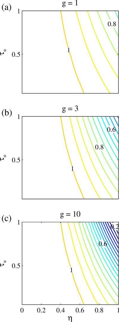
Figure 4: (Color online) The factor $X$ which scales the poloidal impurity flow in the plateau regime, calculated for $\alpha=0$. The horizontal axis is the same for all plots. Contour spacing is 0.05.

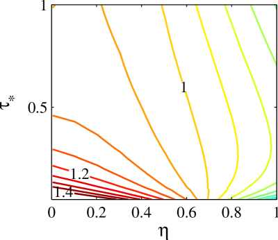
Figure 5: (Color online) The factor $X$ which scales the poloidal impurity flow in the plateau regime for $\alpha=0.25$ and $g=1$. Contour spacing is 0.05.

When the main ions are in the banana regime, the poloidal impurity flow can be calculated using the $K_{z}$ derived in Refs. perbif and fh1 . The result is

$$V_{z\vartheta}^{ban}=\frac{K_{z}B_{\vartheta}}{n_{z}}=\frac{B_{\vartheta}}{n}u\left(\left\langle nb^{2}\right\rangle+\frac{1}{\gamma^{ban}}\right),$$ (32)

where $\gamma^{ban}=eL_{\perp,ban}\left\langle B^{2}\right\rangle u/T_{i}$ and $L_{\perp,ban}^{-1}=-I\left(p_{i}^{\prime}/p_{i}-(3/2)T_{i}^{\prime}/T_{i}\right)$. In the limit of trace impurities and large aspect ratio,

$$u=-0.33f_{c}\frac{I}{e\left\langle B^{2}\right\rangle}\frac{dT_{i}}{d\psi},$$ (33)

and

$$f_{c}\equiv\frac{3\left\langle B^{2}\right\rangle}{4}\int_{0}^{\lambda_{c}}\frac{\lambda d\lambda}{\left\langle n\sqrt{1-\lambda B}\right\rangle}$$ (34)

is the effective fraction of circulating particles. Therefore, in this limit,

$$V_{z\vartheta}^{ban}=-\frac{IB_{\vartheta}}{ne\left\langle B^{2}\right\rangle}\left[\frac{T_{i}}{n_{i0}}\frac{dn_{i0}}{d\psi}+\left(-\frac{1}{2}+0.33f_{c}\left\langle nb^{2}\right\rangle\right)\frac{dT_{i}}{d\psi}\right],$$ (35)

The expression for $u$ in various other limits (arbitrary aspect ratio and high level of impurities) is more complicated and is given in Ref. fh1 .

When the impurity density is nearly constant on a flux surface, (34) gives the conventional result $f_{c}\approx 1-1.46\sqrt{\epsilon}$. For insight into how $f_{c}$ is modified when the impurity density varies significantly on a flux surface, consider the limit $n=\delta(\vartheta-\pi)$ in which the impurities are strongly peaked on the inboard midplane. Then $\left\langle n\sqrt{1-\lambda B}\right\rangle=\sqrt{1-\lambda B_{max}}$ so $f_{c}\approx 1-2\epsilon$.

Similarly, when the main ions are in the Pfirsch-Schlüter regime, the poloidal impurity flow $V_{z\vartheta}^{PS}$ can be calculated using the $K_{z}$ derived in equation (26) of Ref. fh2 . For trace impurities, $V_{z\vartheta}^{PS}$ is found to be

$$V_{z\vartheta}^{PS}=-\frac{IB_{\vartheta}}{ne\left\langle B^{2}\right\rangle}\left[\frac{T_{i}}{n_{i0}}\frac{dn_{i0}}{d\psi}+2.8\left\langle nb^{2}\right\rangle\frac{dT_{i}}{d\psi}\right],$$ (36)

It was found in Refs. perbif and fh1 that when the main ions are in the banana or Pfirsch-Schlüter regimes, the impurities tend to accumulate on the high field side, so $\left\langle nb^{2}\right\rangle>1$. In both regimes, this change decreases the signed $V_{z\vartheta}$, shifting the poloidal impurity flow in the direction of the electron diamagnetic velocity relative to the conventional neoclassical prediction. We can model the impurity density variation as $n=1-(A-1)(A+1)^{-1}\cos\vartheta$, implying $\left\langle nb^{2}\right\rangle=1+\epsilon(A-1)/(A+1)$. As $A$ increases above one, $\left\langle nb^{2}\right\rangle$ increases from one to $1+\epsilon$. For the banana regime, this increase in $\left\langle nb^{2}\right\rangle$ and the aforementioned increase in $f_{c}$ both lead to a decrease in the signed $V_{z\vartheta}$, with the $O(\sqrt{\epsilon})$ increase in $f_{c}$ being the larger of the two effects.

Note that in the method used in this section, the impurity pressure gradient $p_{z}^{\prime}$ does not appear in the formulae for the poloidal impurity flow for any collisionality regime (as it does in, for example, equation (15) of cattosimakov ). In the conventional neoclassical formulae, the $p_{z}^{\prime}$ term is proportional to $1/z$, so the term is formally small in our ordering. The absence of the $p_{z}^{\prime}$ term is related to the fact that the impurity diamagnetic flow was dropped in Eq. (12) in order to make the analysis tractable.

V Conclusions and discussion

In this paper we have investigated the poloidal rearrangement of impurities in the presence of large gradients for the case of background ions in the plateau collisionality regime. The calculation shows that when the temperature scale length is large compared to the density scale length (such that $\eta<0.4-0.6$), the impurities accumulate on the inboard side, whereas they accumulate on the outboard side in the opposite case. In standard tokamak operating regimes, $\eta<0.5$, so impurity accumulation at the inboard side is more likely. However, $\eta$ can be larger than 0.5 in the I-mode regime of Alcator C-Mod Imode , so the strong $\eta$-dependence of $A$ predicted by the theory may be experimentally testable. (Impurity asymmetry in I-mode has not been measured as of this writing.)

One way in which the present calculation could be extended would be to account for the large radial electric field $E_{r}$ which arises in the pedestal. It is found experimentally that the radial electric field in the pedestal can be large enough to make the ${\mbox{\boldmath$E$}}\times{\mbox{\boldmath$B$}}$ drift comparable to $(B_{\theta}/B)v_{i}$, and it was recently shown in pusztai that under these conditions, the plateau-regime ion distribution function can deviate from Eqs. (3-4). Although it would be desirable to include this effect in the present calculation of impurity asymmetry, doing so is not straightforward, for the following reason. Terms in the ion distribution function of order $(\rho_{\theta}/a)\epsilon f_{Mi}$ affect the impurity asymmetry calculation to leading order, as demonstrated by the term with a factor of 3 in Eq. (20), which arises due to the $Q_{r}$ term in Eq. (13). However, the ion distribution function in pusztai is only determined to order $(\rho_{\theta}/a)\epsilon^{0}f_{Mi}$, and to consistently determine all $O(\epsilon)$ corrections, the ion distribution function would need to be found using the full linearized Fokker-Planck collision operator rather than a Krook or pitch-angle scattering model operator.

In all regimes of main-ion collisionality, the poloidal rearrangement of impurities results in changes to the the poloidal impurity flow. These modifications to the flow are of interest because when the main ion collisionality is in the plateau or banana regimes in Alcator C-Mod, impurity velocity in the pedestal is measured to be greater in the electron diamagnetic direction than conventional neoclassical theory predicts marr ; newcmod . When the ions are in the plateau regime, the calculation in this paper shows the impurity flow should be multiplied by the factor $X$ relative to the conventional neoclassical prediction (in which the flow is always in the electron diamagnetic direction.) To explain the observed flows, then, $X$ must be $>1$, which can occur for $\tau_{*}\ll 1$ (as in Figure 5.) When the ions are in the Pfirsch-Schlüter regime, we find the poloidal impurity flow is indeed increased in the direction of the electron diamagnetic velocity due to the increase in $\left\langle nb^{2}\right\rangle$ above one. For banana-regime ions, the flow is shifted in the same direction due to both the increase in $\left\langle nb^{2}\right\rangle$ and also due to the increase in $f_{c}$. However, the shift in the flow is also proportional to the small numerical factor 0.33 in (35), so this effect is likely insufficient to explain the observed discrepancy between the measured and predicted flows. A different calculation, including the $E_{r}$ effects discussed above but neglecting the impurity asymmetry, is discussed in Ref. newcmod ; this calculation can also explain some but not all of the discrepancy. In future work, it may be possible to consistently account for both the $E_{r}$ and impurity asymmetry effects simultaneously to achieve better agreement between the calculated and observed flows.

References

- [1] F. L. Hinton and R. D. Hazeltine, Rev. Mod. Phys 48, 239 (1976).
- [2] S. P. Hirshman and D. J. Sigmar, Nucl. Fusion 21, 1079 (1981).
- [3] K. D. Marr, B. Lipschultz, P. J. Catto, R. M. McDermott, M. L. Reinke, and A. N. Simakov, Plasma Phys. Controlled Fusion 52, 055010 (2010).
- [4] G. Kagan, K. D. Marr, P. J. Catto, M. Landreman, B. Lipschultz, and R. M. McDermott, Plasma Phys. Controlled Fusion 53, 025008 (2011).
- [5] P. Helander, Phys. Plasmas 5, 3999 (1998); The right-hand side of the last equation on p 4002 in this paper should be multiplied by a factor , and the right-hand side of the previous equation (the expression for ) should be multiplied by .
- [6] T. Fülöp and P. Helander, Phys. Plasmas 6, 3066 (1999).
- [7] T. Fülöp and P. Helander, Phys. Plasmas 8, 3305 (2001).
- [8] G. Kagan and P. J. Catto, Plasma Phys. Controlled Fusion 50, 085010 (2008).
- [9] G. Kagan and P. J. Catto, Plasma Phys. Controlled Fusion 52, 055004 (2010).
- [10] I. Pusztai and P. J. Catto, Plasma Phys. Controlled Fusion 52, 075016 (2010).
- [11] P. J. Catto and A. N. Simakov, Phys. Plasmas 13, 052507 (2006).
- [12] D. G. Whyte, A. E. Hubbard, J. W. Hughes, B. Lipschultz, J. E. Rice, E. S. Marmar, M. Greenwald, I. Cziegler, A. Dominguez, T. Golfinopoulos, N. Howard, L. Lin, R. M. McDermott, M. Porkolab, M. L. Reinke, J. Terry, N. Tsujii, S. Wolfe, S. Wukitch, Y. Lin, and the Alcator C-Mod Team, Nucl. Fusion 50, 105005 (2010).