Hysteresis in Anti-Ferromagnetic Random-Field Ising Model at Zero Temperature

Abstract

We study hysteresis in anti-ferromagnetic random-field Ising model at zero temperature. The external field is cycled adiabatically between -$\infty$ and $\infty$. Two different distributions of the random-field are considered, (i) a uniform distribution of width $2\Delta$ centered at the origin, and (ii) a Gaussian distribution with average value zero and standard deviation $\sigma$. In each case the hysteresis loop is determined exactly in one dimension and compared with numerical simulations of the model.

I Introduction

Hysteresis is a non-equilibrium effect commonly observed in systems subjected to a cyclic force  bertotti . It means that the response to a changing force depends on the history of the force. In particular, the response in increasing force is different from that in decreasing force. This is caused by the delay in responding to the force. Theoretically hysteresis should disappear if the force changes sufficiently slowly but this often corresponds to unrealistically long time periods such as the life span of an experimentalist. Several complex and disordered systems like permanent magnets show hysteresis over the longest practical time scales. Experience with spinglasses and other systems containing quenched disorder  young has revealed that the free energy landscape of such systems comprises a large number of local minima (metastable states). The number of local minima is thermodynamically large. The barriers between the local minima are also large compared with the thermal energy of the system. Consequently, in the absence of a driving field the system gets trapped in one of the local minima and is unable to explore the entire phase space over practical time scales. In this situation the thermal relaxation time of the system $\tau$ is much larger than the relaxation time of its constituent units (individual spin-flips) as well as the period $2\pi/\omega$ of the cyclic driving field. A useful approximation is to assume $\tau$ to be infinite or equivalently the system to be at absolute zero temperature. This makes the dynamics of the system deterministic and more amenable to analytic solutions and simulations without compromising the essential physics of the problem. We take the limit $T\rightarrow 0$ before the limit $\omega\rightarrow 0$ to obtain nonvanishing hysteresis in the limit $\omega=0$.

In an extensive and pioneering work Sethna et al  sethna1 ; sethna2 ; dahmen used the random-field Ising model  imryma along with the Glauber dynamics  glauber at zero temperature to study hysteresis in ferromagnets with quenched disorder. They analyzed their model using numerical simulations, mean field theory, Wilson’s renormalization group  wilson , and compared it with experiments. Their model reproduces several experimentally observed features. These include familiar shapes of hysteresis loops, Barkhausen noise  stoner , and return point memory. Interestingly the model predicts the existence of a non-equilibrium critical point on each half of the hysteresis loop. This is based on a Gaussian distribution of the random-field with mean value zero and standard deviation $\sigma$ that plays the role of a tuning parameter in the model. The model may be solved exactly in one dimension and on Bethe lattices of a general coordination number $z$  shukla1 ; shukla2 ; dhar . Above a lower critical coordination number $z$  dhar ; sabhapandit1 there is a critical value $\sigma_{c}$ such that for $\sigma<\sigma_{c}$, each half of the hysteresis loop has a first order jump in the magnetization at some applied field $h$. The size of the jump goes to zero as $\sigma\rightarrow\sigma_{c}$ from below. If $h_{c}$ is the critical field at which the jump vanishes, $\{h_{c},\sigma_{c}\}$ is a non-equilibrium critical point showing scaling of thermodynamic functions and universality of critical exponents in its vicinity. This is reminiscent of equilibrium critical phenomena and appears to have a fair amount of experimental support in the field of hysteresis as well. A generalization of the model  silveira1 ; silveira2 ; shukla3 ; shukla4 to $n$-component ($n>1$) classical spins shows the existence of critical points in the generalized model as well. The critical exponents of the generalized model are in the universality class of the random-field Ising model ($n=1$) if the critical point occurs at a non-zero value of magnetization or the applied field. This is understandable because a non-zero value of magnetization or the applied field picks a unique direction in the system that effectively reduces its symmetry to that of an Ising model. This lends further support to the broad agreement between experiments and predictions of RFIM for hysteresis.

Hysteresis in the anti-ferromagnetic random field Ising model  shukla5 ; shukla6 ; shukla7 ; shukla8 has received relatively little attention as compared to its ferromagnetic counter part  sethna1 ; sethna2 ; dahmen ; dhar ; shukla9 ; shukla10 ; sabhapandit1 ; illa1 ; illa2 ; illa3 ; sabhapandit2 . This is partly due to the difficulty of obtaining analytic solutions in the anti-ferromagnetic case. For the ferromagnetic case, exact expressions for the major and minor hysteresis loops have been obtained in one dimension as well as on a Bethe lattice of coordination number $z$ for a bounded as well as a Gaussian distribution of the quenched field  dhar ; shukla7 ; shukla8 . The distribution of Barkhausen jumps (avalanches) has also been obtained  sabhapandit1 . Several other aspects of the ferromagnetic model have been studied in the mean field theory as well as on periodic lattices  sabhapandit2 ; illa1 ; illa2 ; illa3 . In the anti-ferromagnetic case an expression for the major loop has been obtained  shukla4 in one dimension in case the quenched field has a uniform distribution of width $\Delta$ centered at the origin and $\Delta<|J|$ where $J$ is the anti-ferromagnetic exchange interaction. The purpose of the present paper is to extend this result to $\Delta\geq|J|$ as well. The results presented here are also applicable to unbounded distributions of the quenched random-field such as the Gaussian distribution.

It may appear rather surprising at first sight that there should be any difficulty in solving a one-dimensional Ising model at zero temperature. The difficulty arises primarily from the presence of quenched random fields. Problems with quenched disorder are difficult to analyze analytically. Besides this the spin-flip dynamics with anti-ferromagnetic interactions is more complicated than its ferromagnetic partner. Consider two spin systems of equal size and having the same realization of quenched field distribution. Let one system have ferromagnetic nearest neighbor interaction $J$ and the other an anti-ferromagnetic interaction $-J$. In equilibrium, the ground states of the two systems on a bi-partite lattice are related to each other by symmetry. Evidently no such relation is available between non-equilibrium metastable states of the two systems. An applied field $h_{a}$ increasing adiabatically from $h_{a}=-\infty$ to $h_{a}=\infty$ takes both systems from a stable state with all spins pointing down (i.e. aligned along $h_{a}=-\infty$) to all spins pointing up. Although the end points of the trajectory are the same for both systems but the magnetization paths are different. In particular the number of metastable states along the two paths are different. In the ferromagnetic case, spins tend to flip up in avalanches and do not flip down in increasing field. The anti-ferromagnetic dynamics is marked by the absence of avalanches. This is because a spin flipping up at an applied field $h_{a}$ prevents its neighbors from flipping up at the same field. However, a spin flipping up at $h_{a}$ occasionally causes its neighbor to flip down at $h_{a}$. This is a kind of a reverse avalanche in anti-ferromagnetic dynamics that involves only two spins including the spin that triggers the avalanche. The forward avalanches in the ferromagnetic case, and the reverse avalanches in the anti-ferromagnetic case provide a mechanism for irreversibility in the two models respectively and give rise to hysteresis. Due to the smaller size of reverse avalanches the area of anti-ferromagnetic hysteresis loop is much smaller than the area of ferromagnetic loop. Also the Barkhausen noise on the ferromagnetic hysteresis loop that is caused by large sporadic avalanches is nearly absent in the anti-ferromagnetic case.

The relative difficulty of analyzing anti-ferromagnetic dynamics comes from the fact that it is non-Abelian while the ferromagnetic dynamics is Abelian. This means as follows. Consider an unstable system at an applied field $h_{a}$ such that one or more spins are not aligned along the net field at their site. We relax the system till it is stable. Relaxing the system means checking each spin and flipping it if it is not aligned along the net field at its site. It is an iterative process because flipping a spin may reverse the sign of the net field at its nearest neighbors. We have to continue the relaxation process till each spin in the system is stable. A dynamics is called Abelian if the end result of the relaxation process does not depend on the order in which the spins are relaxed. If the result does depend on the order in which the spins are relaxed it is called non-Abelian. Consider two nearest neighbor spins which are both down but the net field at their sites is positive. If the interaction between the spins is ferromagnetic, the spins can be relaxed in any order and the end result would be that both spins are turned up. This is because turning a spin up makes the net field at its neighbor even more positive so that the neighbor also has to be turned up. This is not the case with anti-ferromagnetic interactions. Turning a spin up decreases the net field at its neighbor and it may decrease it below zero so that the neighbor no longer needs to be turned up when relaxed. Thus the end result may be one spin up and one down. Which one is up depends on which one was turned up first. The anti-ferromagnetic dynamics is therefore non-Abelian. As the stable state at the end of the relaxation process depends on the order in which the unstable spins are relaxed, we have to choose a protocol for the order in which the unstable spins are relaxed. At every step, we choose to relax the most unstable spin in the system i.e. the one whose flipping would lower the energy of the system the most. Locating the most unstable spin at every step of the dynamics is what makes the anti-ferromagnetic model more tedious to analyze theoretically as well as numerically.

Although the aim of the present study is to find an analytic solution of a non-equilibrium problem with quenched disorder, we may mention some connection with experiments. Relaxation dynamics of any complex statistical system belongs to one of two broad categories: (i) where relaxation takes place by avalanches, and (ii) where it proceeds by single localized events. The ferromagnetic random-field Ising model belongs to the category of avalanches. It explains experimental effects such as the Barkhausen noise and the possibility of non-equilibrium critical points. The anti-ferromagnetic random-field Ising models belongs to the second category characterized by the absence of avalanches. Due to the absence of avalanches, we do not expect small changes in the applied field to cause large changes spanning across the system. In other words, we do not expect the response of the system to be critical at any value of the applied field. This rules out the existence of non-equilibrium critical points in anti-ferromagnets. Our calculation shows that the hysteresis loop of an anti-ferromagnet with relatively small quenched disorder (to be defined in the following) has a wasp-waisted shape i.e. constricted in the middle. In the limit of very small disorder the wasp-waisted shape gradually transforms into two hysteresis loops joined by a long and narrow region of almost no hysteresis. For much larger disorder the familiar pot-belly shape of ferromagnetic loops is recovered. Thus the anti-ferromagnets can exhibit a wide variety of shapes of hysteresis loops and this feature of our model is in general conformity with experiments  ayyub ; fukuma ; chiorescu ; fullerton ; waldmann . Anti-ferromagnetic hysteresis loops comprising three loops are also observed in experiments  takanashi ; chew . This too is understandable if our one-dimensional model is extended to lattices with higher coordination number. The anti-ferromagnetic model may also apply to other systems that exhibit glassy dynamics shukla1 ; kisker ; rieger ; ritort ; toninelli characterized by a single localized events.

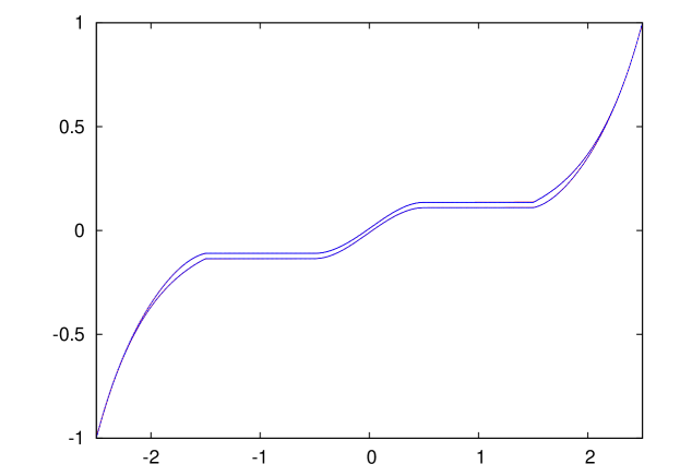
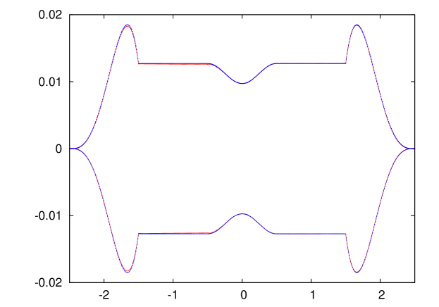
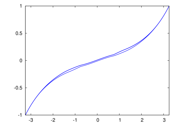
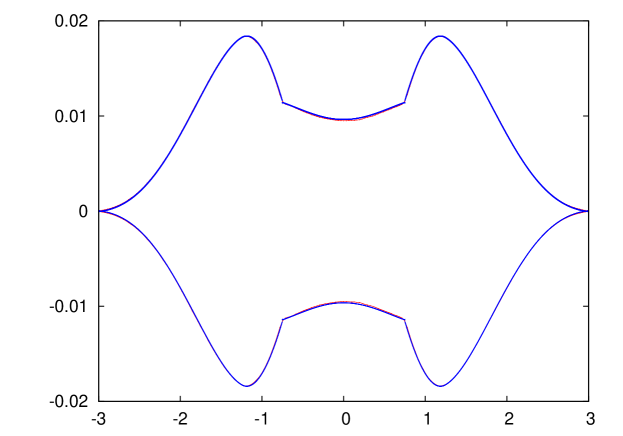
The outline of this paper is as follows. In Section II we define the model for a general distribution of the quenched random-field centered at the origin. We focus on two specific cases: a uniform bounded distribution of width $2\Delta$ and a Gaussian distribution of standard deviation $\sigma$. If $|J|$ is the magnitude of nearest neighbor anti-ferromagnetic interaction, the case $\Delta\leq|J|$ is easier to treat analytically for reasons to be made clear in the following. The case $\Delta>|J|$ is more difficult but comparable to the case of unbounded Gaussian distribution. In Section III, we show numerical results for the hysteresis loop in three representative cases: (i) $\Delta=0.5|J|$, (ii) $\Delta=1.25|J|$, and $\sigma=.5|J|$. Case (i) lies in the ambit of an exact solution obtained earlier  shukla7 ; shukla8 for $\Delta\leq|J|$. In Section IV, we briefly review the earlier result because it is needed to proceed to distributions with $\Delta>|J|$ and the Gaussian distribution. The formalism and presentation of section IV is slightly different from the earlier version  shukla7 ; shukla8 on which it is based in order to make a smoother transition to the following sections. Sections V, VI and VII treat a uniform distribution of arbitrary $\Delta$ and a Gaussian distribution of arbitrary $\sigma$. These sections contain the main results of this paper. Exact expressions for the hysteresis loops are obtained. These have been superimposed on the simulation results shown in figures (1)-(6). The fit between the theory and simulations is quite good as may be expected from an exact solution. Indeed the two are indistinguishable on the scale of the figures. The fact that simulations over a relatively small size of the system agree with the exact result is due to the super-exponential decay of correlations in this system evans . The agreement between simulation and theory also justifies (albeit post facto) the implicit assumption in our analysis that the system is self-averaging.

II The Model

We consider non-equilibrium anti-ferromagnetic random-field Ising model in one dimension at zero temperature. At each site $i$ ($i=1,2,3,\ldots,N$) of a linear lattice, there is an Ising spin $s_{i}=\pm{1}$ which interacts with its nearest neighbors through an anti-ferromagnetic interaction $J$ ($J<0$). A quenched random-field $h_{i}$ as well as a uniform externally applied field $h_{a}$ acts on $s_{i}$. The Hamiltonian of the system is,

$$H=-J\sum_{i}{s_{i}s_{i+1}}-\sum_{i}h_{i}s_{i}-h_{a}\sum_{i}s_{i}$$ (1)

We consider two distributions $\phi(h_{i})$ of the random-field $\{h_{i}\}$:

1. A uniform bounded distribution of width $2\Delta$ centered at the origin,

   $$\phi(h_{i}) =\frac{1}{2\Delta} \mbox{if }[-\Delta\leq h_{i}\leq\Delta]$$ (2)

   $$=0,$$ otherwise.

2. A Gaussian distribution with average zero and standard deviation $\sigma$,

   $$\phi(h_{i})=\frac{1}{\sqrt{2\pi\sigma^{2}}}\left.e^{-\frac{h_{i}^{2}}{2\sigma^{2}}}.\right.$$ (3)

It is convenient to rewrite $H$ in terms of the net field $f_{i}$ acting on spin $s_{i}$,

$$H=-\sum_{i}f_{i}s_{i};\mbox{ }f_{i}=J(s_{i-1}+s_{i+1})+h_{i}+h_{a}$$ (4)

The spins $\{s_{i}(t)=\pm 1\}$ obey discrete-time single-spin-flip Glauber dynamics at zero temperature i.e. $s_{i}(t+1)=\mbox{ sign }f_{i}(t)$. This means a spin flips only if it lowers its energy. It also assumes that if a spin-flip is allowed, it occurs at a rate $\Gamma$ which is much larger than the rate at which the magnetic field $h_{a}$ is varied. Thus all flippable spins relax instantly and $s_{i}(t+1)$ has the same sign as the net local field $f_{i}(t)$ at its site.

$$s_{i}(t+1)=\mbox{ sign }{f_{i}(t)}=\mbox{ sign }[J\{s_{i-1}(t)+s_{i+1}(t)\}+h_{i}+h_{a}(t)]$$ (5)

Iterative application of the above dynamics leads to a fixed point state of the system such that $s_{i}(t+1)=s_{i}(t)$ for each spin $s_{i}(t)$ in the system. The condition of adiabatic variation of the applied field or equivalently the instant relaxation of spins mentioned previously is implemented by holding the applied field constant until a fixed point is reached. The fixed point is a local minimum of the energy (metastable state) of the system. We denote the fixed point value of $s_{i}(t)$ by $s_{i}^{*}$ and characterize the fixed point state by the magnetization $m(h_{a})$ per spin,

$$m(h_{a})=\frac{1}{N}\sum_{i}s_{i}^{*}$$ (6)

Our aim is to find the magnetization $m(h_{a})$ of each metastable state visited by the system as the applied field is cycled adiabatically from $h_{a}=-\infty$ to $h_{a}=\infty$ and back to $h_{a}=-\infty$. We start with $h_{a}=-\infty$ when each spin is necessarily aligned along the applied field i.e. we have a fixed point with $m=-1$. Now we increase $h_{a}$ slowly till some spin becomes unstable and needs to be flipped. We flip this spin and check its neighborhood if any more spins have to be flipped. If any neighbors are flipped, we check their neighbors if they need to be flipped as well. This process is continued till no more spin needs to be flipped i.e. we reach a new fixed point. The applied field is held constant during the passage from the old fixed point to the new. This procedure is continued up to $h_{a}=+\infty$ when $m=1$. The magnetization $m^{u}(h_{a})$ on the upper half of the hysteresis loop when $h_{a}$ is slowly decreased from $h_{a}=+\infty$ to $h_{a}=-\infty$ can be obtained from $m(h_{a})$ by a symmetry relation $m^{u}(h_{a})=-m(-h_{a})$. Therefore the calculation of the lower half of the hysteresis loop suffices to determine the entire hysteresis loop.

III simulations

Computer simulations of the preceding model play a useful role in guiding its analysis and checking the analytic results. Normally we used $10^{3}$ spins on a linear lattice with periodic boundary conditions and used $10^{3}$ independent realizations of the random field distribution to generate the data. The data was binned in $10^{3}$ bins in the applicable range of the applied field and averaged over different realizations of the field distribution. The simulation results shown in figures (1)-(6) and some of the other figures in section VIII were obtained in this way. It took approximately four hours on our 3 GHz desktop to generate the data for each figure. When the estimated probability of an event was very small, say of the order of $10^{-6}$, we performed the corresponding simulation on a larger system, say $10^{6}$ spins, and a smaller number of independent runs, say $10^{2}$. This was to optimize the accuracy of the data and the time taken to generate it. In some cases it was more appropriate to have a larger number of bins. In these cases we worked with the data obtained from a large system of $10^{6}$ spins without binning it. We set $J=-1$, and as mentioned previously we performed simulations for three cases: (i) $\Delta=0.5$, (ii) $\Delta=1.25$, and (iii) $\sigma=0.5$. These values were chosen arbitrarily but represent three broad classes of the analytic results.

III.1 $\Delta=0.5$

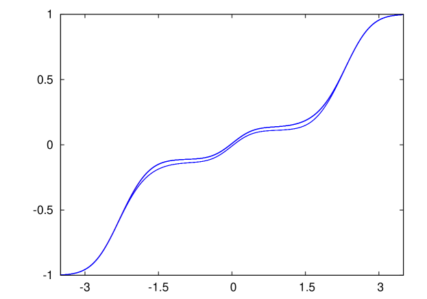
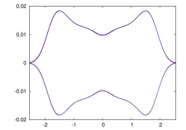
Figure (1) shows the hysteresis loop for $\Delta=0.5$. We see that $m(h_{a})=-1$ if $h_{a}\leq-2|J|-\Delta$, and $m(h_{a})=1$ if $h_{a}\geq 2|J|+\Delta$. The magnetization $m(h_{a})$ rises from -1 to +1 in three steps. We call these steps ramp-I ($h_{a}=-2|J|-\Delta$ to $h_{a}=-2|J|+\Delta$); ramp-II ($h_{a}=-\Delta$ to $h_{a}=+\Delta$); and ramp-III ($h_{a}=2|J|-\Delta$ to $h_{a}=2|J|+\Delta$). The ramps are connected to each other by two plateaus; plateau-I ( $h_{a}=-2|J|+\Delta$ to $h_{a}=-\Delta$); and plateau-II ($h_{a}=+\Delta$ to $h_{a}=2|J|-\Delta$). On the plateaus, the magnetization remains constant even though the applied field continues to increase. Plateaus occur for $\Delta\leq|J|$ (small disorder), and simulations suggest that magnetization on the plateaus is independent of $\Delta$. Numerically, the magnetization on the plateaus is approximately $m^{I}=-.135$ on plateau-I, and $m^{II}=.109$ on plateau-II. The qualitative shape of $m(h_{a})$ is easy to understand. Due to the anti-ferromagnetic interaction between nearest neighbors, spins with both neighbors down are the first to turn up in an increasing applied field. Such spins turn up on ramp-I. Next are the spins with one neighbor up and one down which turn up on ramp-II. Spins with both neighbors up require the largest applied field to turn up, and these turn up on ramp-III. For $\Delta\leq|J|$, the three ramps are well separated from each other. In other words, no spin with $n$ up neighbors ($n=1,2$) can turn up in increasing $h_{a}$ until all spins with $n-1$ up neighbors have turned up. On each ramp, the sequence in which the spins turn up is determined by the distribution of the quenched random field. Spins with large positive quenched field turn up before spins with a lower quenched field. The quenched field lies in the range $-\Delta$ to $+\Delta$. Thus each ramp has a width $2\Delta$ along the axis of the applied field. When a spin turns up on ramp-I, its nearest neighbors are placed in a category so that they cannot turn up before ramp-II. Similarly when a spin turns up on ramp-II, its nearest neighbor which is down cannot turn up before ramp-III. This is essentially the reason for the absence of avalanches in the anti-ferromagnetic RFIM. Occasionally on ramp-II and ramp-III, a spin turning up can cause its nearest neighbor which is already up to turn down. We may call this a reverse avalanche of size unity. There are no long avalanches as in the ferromagnetic model. If there were no reverse flips at all there would be no hysteresis in the model. The smallness of the reverse flips is the reason behind the smallness of the area of the hysteresis loop. In order to highlight the separation of the upper and lower halves of the hysteresis loop we have plotted in figure (2) the relative separation of the two halves relative to their average value. As the majority of the spins turn up one at a time, the calculation of $m(h_{a})$ becomes essentially a matter of sorting quenched random fields in decreasing order on each ramp. The difficulty arises from the fact that a posteriori distribution of random fields on unflipped spins that are next to a flipped spin is significantly different from the initial uniform distribution. The main problem is to calculate this a posteriori probability distribution of random fields on unflipped spin sites.

III.2 $\Delta=1.25$

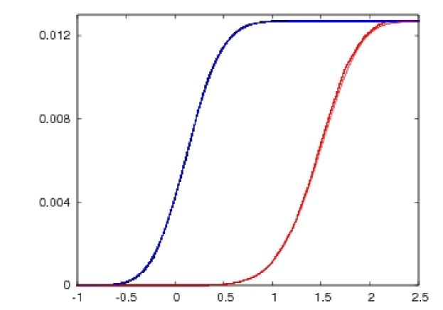
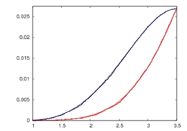
Figure (3) shows the hysteresis loop for $\Delta=1.25$. We see that the three ramps comprising the hysteresis loop in figure (1) have lost their individual identity. If $\Delta>|J|$, a spin with one neighbor up can turn up on the lower hysteresis loop before all spins with both neighbors have turned up. This makes the analysis of the dynamics more complex. We shall take it up in Section V and Section VI. Figure (4) is a magnified version of figure (3). It shows the relative separation of the two halves from their average value at a given applied field.

III.3 $\sigma=0.5$

Figure (5) shows the hysteresis loop for $\sigma=0.5$ for a Gaussian distribution of the random field. The Gaussian distribution is an unbounded distribution. Therefore we may not expect the hysteresis loop to comprise of sharp ramps and plateaus as in figure (1). However, notice the qualitative similarity between figure (5) for $\sigma=0.5$ and figure (1) for $\Delta=0.5$ sans the sharp edges in figure (1). The general analysis presented in sections V, VI, VII applies equally to a uniform distribution with any value of $\Delta$ and a Gaussian distribution for any value of $\sigma$. Figure (6) is a magnified version of figure (5) showing the relative separation of the two halves of the hysteresis loop from their average value at a given applied field. In view of the smallness of the area of the anti-ferromagnetic hysteresis loop, the magnified loops are better suited for comparing the fit between simulation and the theory to be presented in the following sections.

IV Bounded distribution of quenched field with $\Delta\leq|J|$

If $\Delta\leq|J|$ and the applied field $h_{a}$ is increased adiabatically from $-\infty$ to $\infty$, the spins with both neighbors down flip up first (ramp-I). Next are those with one neighbor up and one down (ramp-II). The last category of spins to flip up are those with both neighbors up (ramp-III). The ramps are separated by plateau-I and plateau-II. The width of the plateaus along the applied field axis decreases with increasing $\Delta$ and goes to zero as $\Delta\rightarrow|J|$. Magnetization on ramp-I was determined in reference  shukla5 by exploiting a similarity between this problem and the problem of random sequential adsorption(RSA) evans . The rate equations of the RSA problem were used to determine $m(h_{a})$ on ramp-I, but they could not determine $m(h_{a})$ on ramp-II and ramp-III. A different approach was introduced in  shukla6 ; shukla7 which determined magnetization on all three ramps for $\Delta\leq|J|$. We recall this approach briefly because it serves as the starting point for analyzing magnetization curves for $\Delta>|J|$ as well as for a Gaussian distribution of random-fields. The following subsections contain the main results obtained in references  shukla6 ; shukla7 with some reworking of notation and formalism.

IV.1 Ramp-I

The analytical results for the magnetization on ramp-I are conveniently expressed in terms of three quantities $p_{0}(h_{a})$, $p_{1}(h_{a})$, and $p_{2}(h_{a})$. These are the probabilities that a spin which has quenched field $h_{i}$ and which has respectively zero, one, or two nearest neighbors up can flip up at applied field $h_{a}$. Thus,

$$p_{n}(h_{a})=\int_{-2(1-n)|J|-h_{a}}^{\infty}\phi(h_{i})dh_{i}\mbox{ }(n=0,1,2)$$ (7)

As the applied field increases adiabatically from $h_{a}=-\infty$ to $h_{a}=\infty$, spins with both neighbors down begin to flip up at $h_{a}=-2|J|-\Delta$ and continue to flip up till $h_{a}=-2|J|+\Delta$ at which stage ramp-I is completed and there are no down spins whose neighbors are also down. The fraction of up spins on ramp-I at an arbitrary applied field $h_{a}$ is given by,

$$P_{\uparrow}^{I}(h_{a})=\frac{1}{2}[1-e^{-2p_{0}(h_{a})}],$$ (8)

The central object in the calculation of $P_{\uparrow}^{I}(h_{a})$ is the probability (per site) of finding a pair of adjacent down spins on ramp-I at applied field $h_{a}$. We denote this object by the symbol $P_{\downarrow\downarrow}^{I}(h_{a})$. It is calculated as follows. Imagine coloring all sites with $h_{i}+2|J|+h_{a}\geq 0$ black, and all sites with $h_{i}+2|J|+h_{a}<0$ white. Consider two adjacent down spins A and B shown in Figure (7). The sites A and B can be both white, both black, or mixed. Given that A is down, it is clear that the state of B can only be influenced by the evolution of the system to the right of B. Similarly, given that B is down, the state of A can only be influenced by the evolution of the system to the left of A. We shall refer to this as the principle of conditional independence mityushin . It requires

$$P_{\downarrow\downarrow}^{I}(h_{a})=P(A\downarrow|B\downarrow)P(B\downarrow|A\downarrow)$$ (9)

where $P(A\downarrow|B\downarrow)$ is the probability that spin at site A is down given that spin at B is down, and $P(B\downarrow|A\downarrow)$ is the probability that B is down given that A is down. We take up the calculation of $P(B\downarrow|A\downarrow)$. If B is a white site, $P(B\downarrow|A\downarrow)=1$ because white sites have not been relaxed from their initial state. If B is a black site and the site to the right of B is a white site then $P(B\downarrow|A\downarrow)=0$. In general $P(B\downarrow|A\downarrow)$ depends on the length of the string of black sites to the right of B. Suppose B is a black site, and there are $(n-1)$ additional black sites to the right of B. In this case, the probability $P^{n}_{B}$ that B is down satisfies the following recursion relation,

$$P^{n}_{B}=\frac{1}{n}P^{n-2}_{B}+(1-\frac{1}{n})P^{n-1}_{B}$$ (10)

The rationale for the above recursion relation is as follows. Let the black site farthest from B on the right be labeled as the $n$-$th$ site. Any of the $n$ sites could flip first. The probability that the $n$-$th$ site flips first is therefore equal to $\frac{1}{n}$. If this happens, ($n$-1)-$th$ site is prevented from flipping up on ramp-I. The probability that B is down is now reduced to the probability that the end point of a chain of ($n$-2) black sites is down i.e. $P_{B}^{n-2}$. This accounts for the first term in equation (10). The probability that $n$-$th$ site is not the first site to flip up is equal to $(1-\frac{1}{n})$. Given this situation, the probability that B is down is equal to the probability that the end of a string of ($n$-1) black sites is down. This accounts for the second term in equation (10). We can rewrite the recursion relation (10) as

$$(P^{n}_{B}-P^{n-1}_{B})=-\frac{1}{n}[P^{n-1}_{B}-P^{n-2}_{B}]$$ (11)

It has the solution,

$$P^{n}_{B}=\sum^{n}_{m=0}\frac{(-1)^{m}}{m!}$$ (12)

Summing over various possible values of $n$ with appropriate weight, we get

$$P(B\downarrow|A\downarrow) = \sum^{\infty}_{n=0}\sum^{n}_{m=0}\frac{(-1)^{m}}{m!}{p_{0}^{n}}(1-p_{0})$$ (13)

$$=\sum^{\infty}_{m=0}\frac{(-1)^{m}}{m!}(1-p_{0})\sum^{\infty}_{n=m}p_{0}^{n}=\sum^{\infty}_{m=0}\frac{(-p_{0})^{m}}{m!}=e^{-p_{0}}$$

In the above array of equations, $p_{0}$ stands for $p_{0}(h_{a})$. Thus,

$$P_{\downarrow\downarrow}^{I}=e^{-2p_{0}(h_{a})}$$ (14)

Let $P_{\downarrow}^{I}$ be the probability per site of finding a down spin and $P_{\downarrow\uparrow}^{I}$ the probability per site of finding a down spin which is followed by an up spin. Clearly,

$$P_{\downarrow}^{I}=P_{\downarrow\downarrow}^{I}+P_{\downarrow\uparrow}^{I}=1-P_{\uparrow}^{I}$$ (15)

Keeping in mind that on ramp-I an up spin must be preceded (as well as followed) by a down spin, we get $P_{\downarrow\uparrow}^{I}=P_{\uparrow}^{I}$. Thus,

$$P_{\uparrow}^{I}=1-P_{\downarrow\downarrow}^{I}-P_{\uparrow}^{I}$$

or,

$$P_{\uparrow}^{I}=\frac{1}{2}[1-P_{\downarrow\downarrow}^{I}]=\frac{1}{2}[1-e^{-2p_{0}(h_{a})}]$$ (16)

The magnetization on ramp-I is given by

$$m^{I}(h)=2P_{\uparrow}^{I}(h)-1=-e^{-2p_{0}(h_{a})}$$ (17)

The exact value of the magnetization on plateau-I is equal to $-\frac{1}{e^{2}}$ which is approximately equal to -.135.

IV.2 Plateau-I

Plateau-I contains down spins in singlets and doublets punctuated by up spins. Each spin in a doublet has one neighbor up and one down. Therefore the net field on it is simply the sum of the random field $h_{i}$ on its site and the applied field $h_{a}$. It turns up when $h_{i}+h_{a}\geq 0$. The random field lies in the range $-\Delta<{h_{i}}<+\Delta$. Therefore an applied field smaller than $-\Delta$ is sufficiently negative to pin down all doublets. This accounts for the range $(-2|J|+\Delta)<h_{a}<{-\Delta}$ where the magnetization shows a plateau. In each doublet, the spin with the larger quenched field $h_{i}$ flips up on ramp-II when $h_{i}+h_{a}\geq 0$. The spin with the smaller quenched field then becomes a singlet which does not flip up before ramp-III. Thus, in order to find the form of ramp-II, we need to find the a posteriori distribution of quenched random fields on the doublets.

Consider a doublet on plateau-I as shown in Figure (8). The doublet sites are denoted as 1 and 2, and the quenched random fields on these sites are $h_{1}$ and $h_{2}$. The a posteriori probability distributions of $h_{1}$ and $h_{2}$ will be identical by symmetry. These distributions $\tilde{\phi}(h_{1})$ and $\tilde{\phi}(h_{2})$ are determined by the relaxation process on ramp-I. If the doublet survives up to plateau-I it must exist on ramp-I. Consider ramp-I at an applied field $h_{a}$. Given that site-2 is down at this point, the probability that site-1 is also down is equal to $e^{-p_{0}(h)}$. Site-1 may be down because (i) it is a white site i.e. $h_{1}+2|J|+h_{a}\leq 0$ and therefore it could not turn up even if both its nearest neighbors were down, or (ii) it is a black site but blocked from turning up by its neighbor that has turned up before it. The probability that it is a white site is equal to $1-p_{0}(h_{a})$. Therefore the probability that it is a black site but down at $h_{a}$ is equal to $e^{-p_{0}(h_{a})}-\{1-p_{0}(h_{a})\}$. This means,

$$Prob(1\downarrow|2\downarrow;h_{1}+2|J|+h_{a}\geq 0)=\int_{-2|J|-h_{a}}^{\Delta}\tilde{\phi}(h_{1})dh_{1}=\left[e^{-p_{0}(h_{a})}-\{1-p_{0}(h_{a})\}\right].$$ (18)

${\tilde{\phi}(h_{1})}$ is obtained by taking the derivative of the above expression. We get,

$$\tilde{\phi}(h_{1})dh_{1}=[1-e^{-p_{0}(-h_{1}-2|J|)}]\phi(h_{1})dh_{1}$$ (19)

Assuming $h_{1}>h_{2}$, site-1 would turn up on ramp-II when $h_{1}+h_{a}=0$. The density of sites on ramp-II at this value of the applied field is given by,

$$\tilde{\phi}(-h_{a})dh_{a}=[1-e^{-p_{0}(h_{a}-2|J|)}]\phi(-h_{a})dh_{a}=[1-e^{-p_{1}(h_{a})}]\phi(-h_{a})dh_{a}$$ (20)

We now address an issue which is crucial for determining ramp-II correctly. This concerns two adjacent doublets as shown in Figure (9). What is the probability per site of observing this object on ramp-I? A doublet has an important property. It separates the lattice into two parts (one on each side of the doublet) which have evolved uninfluenced by each other. Thus, we can separate Figure (9) into three parts as enclosed in the dashed boxes. Evolution inside each box has remained shielded from the outside. The evolution in the middle box requires that site 3 flips up before site 2 or site 4. The probability for this event is equal to $\frac{1}{3}$. Given that site 2 is down, the probability that site 1 is down is equal to $e^{-p_{0}(h_{a})}$. Similarly, given that site 4 is down the probability that site 5 is down is equal to $e^{-p_{0}(h_{a})}$. Thus the probability per site of observing two adjacent doublets on ramp-I at an applied field $h_{a}$ is equal to $\frac{1}{3}e^{-2p_{0}(h_{a})}$. Note that it is quite different from the square of the probability of finding a single doublet! Let $h_{1}$, $h_{2}$, $h_{3}$, $h_{4}$ and $h_{5}$ denote the quenched fields at sites 1, 2, 3, 4, and 5 respectively. We are interested in the case $h_{2}>h_{1}$, and $h_{4}>h_{5}$, and ask what are a posteriori distribution of fields $h_{1},h_{2},\ldots,h_{5}$ on ramp-II. Let the probability that $h_{i}(i=1,\ldots,5)$ lies in the range $[-h_{a}-dh_{a},-h_{a}]$ on ramp-II be denoted by $\rho_{i}(-h_{a})dh_{a}$. The distributions of $h_{1}$ and $h_{5}$ are given by,

$$\rho_{1}(-h_{a})=\frac{\{1-e^{-p_{1}(h_{a})}\}}{e^{-p_{0}(h_{a})}}\phi(-h_{a})$$ (21)

$$\rho_{5}(-h_{a})=\frac{\{1-e^{-p_{1}(h_{a})}\}}{e^{-p_{0}(h_{a})}}\phi(-h_{a})$$ (22)

Equation (21) is obtained as follows. If sites 1 and 2 are down on plateau-I, they must have been down all along ramp-I. Given that site 2 is down on ramp-I, the probability that site-1 is down is equal to $e^{-p_{0}(h_{a})}$. This accounts for the denominator. The numerator gives the a posteriori probability distribution of the quenched field at site 1 on the lines of the preceding discussion with reference to figure (8). Equation (22) is written similarly. Note that the distributions $\rho_{1}(h_{i})$ and $\rho_{5}(h_{i})$ are each normalized to unity. Next we turn to the distributions of $h_{2}$, $h_{3}$, and $h_{4}$. As stated previously, $h_{2}>h_{1}$ and $h_{4}>h_{5}$ so we are looking at the case where $h_{2}$ and $h_{4}$ flip up on ramp-II. We may assume without loss of generality that $h_{4}>h_{2}$. Let $h_{4}$ flips up on ramp-II at applied field $h_{a}$ i.e. $h_{4}+h_{a}=0$. The probability for this is equal to $\phi(-h_{a})p_{1}(h_{a})\{1-p_{1}(h_{a})\}$; the three multiplicative factors giving respectively the probability that $h_{4}=-h_{a}$, site 3 is up at $h_{a}$, and site 2 is down at $h_{a}$. Thus,

$$\rho_{4}(-h_{a})=6p_{1}(h_{a})\{1-p_{1}(h_{a})\}\phi(-h_{a})$$ (23)

The factor of 6 on the rhs arises as follows. At $h_{a}$ on ramp-II site 2 will be down and sites 3 and 4 will be up at $h_{a}$ given that at an earlier field $h_{a}-2|J|$ on ramp-I site 3 had flipped up before 2 and 4 with probability $\frac{1}{3}$. The site flipping up on ramp-II may be to the left of the central site or to its right. This gives an additional factor of 2.

The distribution of $h_{2}$ is obtained similarly. We find,

$$\rho_{2}(-h_{a})=3p_{1}^{2}(h_{a})\phi(-h_{a})$$ (24)

IV.3 Ramp-II

Ramp-II is determined by the combination of two terms. The dominant term is the increase in magnetization due to the decrease in the number of doublets. When a doublet disappears, it adds an extra up spin in the system which increases the magnetization. Occasionally, a disappearing doublet creates a string of three up spins. A triplet of up spins is unstable on ramp-II if $\Delta\leq|J|$ and therefore the central spin of the triplet flips down as soon as the triplet is created. This decreases the magnetization. In the following, we calculate the above two terms separately. Refer to figure (8) for calculating the first term. Let us assume $h_{1}<h_{2}$. The a posteriori distribution of fields $h_{1}$ and $h_{2}$ in figure (8) are the same as $\rho_{1}(h_{1})$ in figure (9). The probability that the doublet disappears at $h_{2}+h_{a}=0$ on ramp-II is given by

$$P_{\uparrow\uparrow}^{II}=2e^{-2p_{0}(h_{a})}\int_{-h_{a}}^{\infty}\rho_{1}(h_{2})dh_{2}\int_{-\infty}^{h_{2}}\rho_{1}(h_{1})dh_{1}$$ (25)

The factor $e^{-2p_{0}(h_{a})}$ is the probability per site of finding a doublet at $h_{a}$ before any of them have been relaxed. The factor 2 takes care of the fact that either $h_{1}$ or $h_{2}$ may be the larger field although the expression is written on the assumption that site 2 flips up first. When a doublet disappears, a pair of adjacent up spins is created. This is the reason for the choice of the subscript on $P_{\uparrow\uparrow}^{II}$. The superscript indicates that the probability refers to ramp-II. We obtain,

$$P_{\uparrow\uparrow}^{II}=e^{-2p_{0}(h_{a})}\left.{\left\{\int_{-\infty}^{h_{2}}\rho_{1}(h_{1})dh_{1}\right\}}^{2}\right|^{h_{2}=\infty}_{h_{2}=-h_{a}}$$ (26)

For $\Delta\leq|J|$, $p_{0}(h_{a})=1$ if $p_{1}(h_{a})>0$. Therefore,

$$P_{\uparrow\uparrow}^{II}=\frac{1}{e^{2}}-\left[\left(1+e^{-1}\right)-\left\{p_{1}(h_{a})+e^{-p_{1}(h_{a})}\right\}\right]^{2}$$ (27)

We now calculate the fraction of (unstable) up triplets on ramp-II. Refer to figure (9) with the assumption that $h_{2}<h_{4}$. An up triplet forms when $h_{2}+h_{a}=0$. The cumulative fraction of up triplets is given by,

$$P_{\uparrow\uparrow\uparrow}^{II}=\frac{1}{3}e^{-2p_{0}(h_{a})}\int_{-h_{a}}^{\infty}\rho_{2}(h_{2})dh_{2}\int_{-\infty}^{h_{2}}\rho_{1}(h_{1})dh_{1}\int_{h_{2}}^{\infty}\tilde{\rho}_{4}(h_{4})dh_{4}\int_{-\infty}^{h_{4}}\rho_{5}(h_{5})dh_{5}$$ (28)

The two factors before the integrals give the probability per site of finding the object shown in Figure (9). These take into account the condition that $h_{3}>h_{4}$. The next two integrals give the probability that $h_{2}+h_{a}=0$ and $h_{1}<h_{2}$. When $h_{2}$ is in the range $-h_{a}$ and $-h_{a}-\delta h_{a}$, $h_{4}$ can be anywhere in the range $h_{2}$ to $\infty$. Let $\tilde{\rho_{4}(h_{4})}$ be the density of $h_{4}$ in this range. Clearly,

$$\rho_{2}(h_{2})=\int_{h_{2}}^{\infty}\tilde{\rho}_{4}(h_{4})dh_{4},\mbox{ or }\tilde{\rho}_{4}(h_{i})=-\frac{d\rho_{2}(h_{i})}{dh_{i}}$$ (29)

.

The integrals in equation (28) can be evaluated exactly for a uniform distribution. We get a non-zero contribution only if $p_{1}(h_{a})>0$. If $\Delta<|J|$ and $p_{1}(h_{a})>0$ then we must necessarily have $p_{0}(h_{a})=1$. Thus we get,

$$P_{\uparrow\uparrow\uparrow}^{II}=\frac{1}{3}\left[\frac{3}{2}+\frac{6}{e}-6\left\{1+\frac{1}{e}\right\}p_{1}(h_{a})+3p_{1}^{2}(h_{a})+{\left\{1+\frac{1}{e}\right\}}^{2}p_{1}^{3}(h_{a})-\frac{5}{4}\left\{1+\frac{1}{e}\right\}p_{1}^{4}(h_{a})+\frac{2}{5}p_{1}^{5}(h_{a})\right.\\$$

$$\left.-\left\{6\left(1+\frac{1}{e}\right)-6p_{1}(h_{a})-3\left(1+\frac{1}{e}\right)p_{1}^{2}(h_{a})+2p_{1}^{3}(h_{a})\right\}e^{-p_{1}(h_{a})}+\left\{\frac{9}{2}+3p_{1}(h_{a})\right\}e^{-2p_{1}(h_{a})}\right]$$

Putting the various terms together, the probability that a randomly chosen spin on the lattice is up on ramp-II is given by

$$P_{\uparrow}^{II}(h_{a})=\frac{1}{2}[1-e^{-2}]+P_{\uparrow\uparrow}^{II}(h_{a})-P_{\uparrow\uparrow\uparrow}^{II}(h_{a})$$ (30)

The magnetization on ramp-II is given by

$$m^{II}(h_{a})=2P_{\uparrow}^{II}(h_{a})-1$$ (31)

The magnetization on plateau-II is equal to,

$$m^{II}=\left[\frac{27}{30}-\frac{7}{6}e^{-1}-\frac{8}{3}e^{-2}\right]=.109\mbox{ (approximately) }$$ (32)

IV.4 Plateau-II

Each down spin on plateau-II is a singlet. However, there are three different classes of singlets: the singlets formed on ramp-I; singlets formed on ramp-II by a vanishing doublet; and finally the singlets formed on ramp-II by the unstable central spin of an up triplet flipping down. The a posteriori distribution of random field is different for each class. Let $\rho^{II}_{a}$, $\rho^{II}_{b}$, and $\rho^{II}_{c}$ denote the density of random fields in the three cases and $P^{II}_{a}$, $P^{II}_{b}$, and $P^{II}_{c}$ be the probability of finding the corresponding singlet at applied field $h_{a}$on plateau-II.

$$P^{II}_{x}(h_{a})=\int_{-h_{a}}^{\infty}\rho^{II}_{x}(h_{i})dh_{i},\mbox{ x=a, b, c }$$ (33)

It is useful to think of singlets in each class as being black or white on the ramp on which they are created. Suppose a singlet is created on ramp-I at applied field $h_{a}^{\prime}$. It is created black if $h_{i}+2|J|+h_{a}^{\prime}\geq 0$, and white if $h_{i}+2|J|+h_{a}^{\prime}<0$ where $h_{i}$ is the quenched random field at the singlet site. If a singlet is black at applied field $h_{a}^{\prime}$ then it is also black at fields greater than $h_{a}^{\prime}$. A black singlet on ramp-I at $h_{a}^{\prime}$ will turn up on ramp-III at $h_{a}=h_{a}^{\prime}+4|J|$. Therefore if we know the fraction of black singlets on ramp-I we can calculate how they are destroyed on ramp-III.

The fraction of black singlets created on ramp-I is given by,

$$P^{II}_{a}(h_{a}^{\prime})=p_{0}(h_{a}^{\prime})-\frac{1}{2}\left[1-e^{-2p_{0}(h_{a}^{\prime})}\right]-2e^{-p_{0}(h_{a}^{\prime})}\left[e^{-p_{0}(h_{a}^{\prime})}-\{1-p_{0}(h_{a}^{\prime})\}\right]$$ (34)

The explanation of the above equation is as follows. Imagine ordering the sites of the lattice in order of decreasing quenched field on the site. When all sites with $h_{i}+2|J|+h_{a}^{\prime}\geq 0$ have been relaxed, the fraction of the relaxed sites is equal to $p_{0}(h_{a}^{\prime})$ (the black sites). This fraction is made of the up sites (the second term on the right), black doublet sites (the last term), and the black singlets. Hence the equation for $P^{II}_{1}(h_{a}^{\prime})$. The last term is written as follows. In each doublet, there are two sites from which we can choose one. This accounts for the factor 2. The quantity in the square bracket gives the probability that the chosen site is black, and $e^{-p_{0}(h_{a}^{\prime})}$ is the probability that the other site can have any allowed value of the quenched field.

It is instructive to derive equation (34) by an alternate and more direct method as well. We note that a pair of down spins on the chain has to be followed by a down spin or an up spin, i.e. $P_{\downarrow\downarrow}=P_{\downarrow\downarrow\downarrow}+P_{\downarrow\downarrow\uparrow}$. Similarly, $P_{\uparrow\downarrow\downarrow}+P_{\downarrow\downarrow\downarrow}=P_{\downarrow\downarrow}$. Thus,

$$P_{\uparrow\downarrow\downarrow}(h_{a}^{\prime})=P_{\downarrow\downarrow\uparrow}(h_{a}^{\prime})=P_{\downarrow\downarrow}(h_{a}^{\prime})-P_{\downarrow\downarrow\downarrow}(h_{a}^{\prime})=e^{-2p_{0}(h_{a}^{\prime})}-\{1-p_{0}(h_{a}^{\prime})\}e^{-2p_{0}(h_{a}^{\prime})}=p_{0}(h_{a}^{\prime})e^{-2p_{0}(h_{a}^{\prime})}$$ (35)

We can obtain the fraction of singlets $P_{\uparrow\downarrow\uparrow}$ from $P_{\uparrow\downarrow\downarrow}$ and $P_{\downarrow\downarrow\uparrow}$ by calculating the probability that the down spin at either end flips up under a $p_{0}$ process.

$$P_{\uparrow\downarrow\uparrow}(h_{a}^{\prime})=2\int_{-\infty}^{h_{a}^{\prime}}P_{\uparrow\downarrow\downarrow}(h_{a}^{\prime\prime})\phi(-2|J|-h_{a}^{\prime\prime})dh_{a}^{\prime\prime}=2\int_{0}^{p_{0}(h_{a}^{\prime})}e^{-2p_{0}}p_{0}dp_{0}=\frac{1}{2}\left[1-e^{-2p_{0}(h_{a}^{\prime})}\right]-p_{0}(h_{a}^{\prime})e^{-2p_{0}(h_{a}^{\prime})}$$ (36)

The above expression gives the total fraction of singlets on ramp-I which include black $(h_{i}+2|J|+h_{a}^{\prime}\geq 0)$ as well as white $(h_{i}+2|J|+h_{a}^{\prime}<0)$ singlets. The fraction of white singlets is given by,

$$P_{\uparrow\downarrow\uparrow}^{white}(h_{a}^{\prime})=\{1-p_{0}(h_{a}^{\prime})\}[1-e^{-p_{0}(h_{a}^{\prime})}]^{2}$$ (37)

The first factor on the rhs gives the probability that the central site is white. Given that the central site is white, the probability that its neighbor is up is equal to $1-e^{-p_{0}(h_{a}^{\prime})}$. The probability that both neighbors are up is equal to $[1-e^{-p_{0}(h_{a}^{\prime})}]^{2}$. Thus,

$$P_{\uparrow\downarrow\uparrow}^{black}(h_{a}^{\prime})=P_{\uparrow\downarrow\uparrow}(h_{a}^{\prime})-P_{\uparrow\downarrow\uparrow}^{white}(h_{a}^{\prime})=p_{0}(h_{a}^{\prime})-\frac{1}{2}\left[1-e^{-2p_{0}(h_{a}^{\prime})}\right]-2e^{-p_{0}(h_{a}^{\prime})}\left[e^{-p_{0}(h_{a}^{\prime})}-\{1-p_{0}(h_{a}^{\prime})\}\right]$$ (38)

The fraction of black singlets on ramp-II ($h_{i}+h_{a}^{\prime\prime}\geq 0$) generated by vanishing doublets is given by,

$$P^{II}_{b}(h_{a}^{\prime\prime})=\left[e^{-p_{1}(h_{a}^{\prime\prime})}-\{1-p_{1}(h_{a}^{\prime\prime})\}\right]^{2}$$ (39)

The above equation is easily understood. It is the probability that both sites of the doublet are black. If both sites of the doublet are black, the one with higher random field must flip up on ramp-II leaving us with a singlet on plateau-II which is black.

The fraction of black singlets created by unstable triplets requires the calculation of triplets. We have calculated the fraction of triplets as they are formed on ramp-II. What we need now is a similar but different calculation. The point can be understood with a reference to Figure (9). Recall that $h_{3}\geq h_{4}\geq h_{2}$. On ramp-II, we needed the fraction of triplets with $h_{2}+h_{a}^{\prime\prime}\geq 0$, because the formation of triplets is controlled by this threshold. The restoration of the triplets on ramp-III is controlled by the condition $h_{3}-2|J|+h_{a}\geq 0$. Keeping in mind that we want $h_{1}\leq h_{2}$, and $h_{5}\leq h_{4}$, the probability that $h_{3}-2|J|+h_{a}\geq 0$ is given by,

$$P^{II}_{c}(h_{a})=2\int_{-h_{a}+2|J|}^{\infty}\phi(h_{3})dh_{3}\int_{-\infty}^{h_{3}}\rho_{4}(h_{4})dh_{4}\int_{-\infty}^{h_{4}}\rho_{5}(h_{5})dh_{5}\int_{-\infty}^{h_{4}}\rho_{2}(h_{2})dh_{2}\int_{-\infty}^{h_{2}}\rho_{1}(h_{1})dh_{1}$$

Using $p_{0}(h_{a})=1$ and $p_{1}(h_{a})=1$ on plateau-II we get,

$$P^{II}_{c}(h_{a})= -\left(1+\frac{2}{e}\right)+\left[\frac{1}{4}+\frac{2}{e}+\frac{4}{e^{2}}\right]p_{2}(h_{a})-\frac{1}{2}\left[1+\frac{5}{e}+\frac{4}{e^{2}}\right]p_{2}^{2}(h_{a})+\frac{1}{3}\left[\frac{3}{2}+\frac{4}{e}+\frac{1}{e^{2}}\right]p_{2}^{3}(h_{a})$$ (40)

$$-\frac{1}{4}\left[1+\frac{1}{e}\right]p_{2}^{4}(h_{a})+\frac{1}{20}p_{2}^{5}(h_{a})+\left[1+\frac{2}{e}\right]e^{-p_{2}(h_{a})}-\frac{2}{e}p_{2}(h_{a})e^{-p_{2}(h_{a})}+p_{2}^{2}(h_{a})e^{-p_{2}(h_{a})}$$

$$+\frac{1}{2}\left[1-e^{-2p_{2}(h_{a})}\right]$$

IV.5 Ramp-III

The rise of magnetization on ramp-III is due to singlet sites turning up in increasing field. At the start of ramp-III there are three categories of singlets present on plateau-II, and we have classified each of them conveniently into black and white singlets. The fraction of singlets on plateau-II that turn up at $h_{a}$ on ramp-III is given by the fraction of black singlets in each of the three categories:

$$P^{III}(h_{a})=P^{III}_{a}(h_{a})+P^{III}_{b}(h_{a})+P^{III}_{c}(h_{a})$$ (41)

However the calculation of magnetization on ramp-III turns out to be a bit more complicated. There is a new twist. Frequently when an original singlet site on plateau-II turns up on ramp-III its nearest neighbor turns down. We call this the creation of a new singlet on ramp-III. The newly created singlet site would turn up at a larger applied field on ramp-III. We shall call this event the destruction of the newly created singlet. We have to calculate the newly created singlets and their destruction before the magnetization on ramp-III may be obtained. It should be noted that this means that some sites flip three times in the course of a monotonic increase of applied field from $-\infty$ to $\infty$. However, no site flips more than three times.

When does a vanishing singlet on ramp-III create a new singlet on an adjacent site? Consider the singlet at site 3 in figure 10. Suppose site 3 flips up at $h_{a}$, i.e. $h_{3}-2|J|+h_{a}=0$. Now the net field on site 2 is equal to $h_{2}+h_{a}$. This is necessarily positive because $h_{2}+2|J|-h_{3}\geq 0$ if $\Delta\leq|J|$. Thus site 2 would stay up after site 3 flips up. Consider site 4. After site 3 has turned up the net field at site 4 is equal to $h_{4}-2|J|+h_{a}$. Thus site 4 will turn down if $h_{4}<h_{3}$. Site 3 will stay up even if site 4 turns down because $h_{3}+h_{a}>0$. These considerations can be put in the form of two guiding rules. When a singlet turns up on ramp-III, (i) its nearest neighbor stays up if the next nearest neighbor is down, and $\Delta\leq|J|$, (ii) its nearest neighbor turns down if it has less quenched field than the singlet and the next nearest neighbor is up. Detailed considerations show that only the singlets created on ramp-I fall under the purview of these rules. Therefore we focus on the singlets present on plateau-I. Specifically we focus on the configurations shown in figure (11) and figure (12). In each of these figures a new singlet is created on site 3 when the singlet on site 2 is destroyed. The two figures make different contributions because of the role played by the next nearest neighbor of the singlet on the side of the newly created singlet.

The a posteriori distribution of the quenched field at site 2 is given by

$$\tilde{\tilde{\phi}}(h_{2})=\left[1-e^{-p_{2}(-h_{2}+2|J|)}\right]\phi(h_{2})$$ (42)

The contributions of figure (11) to the fraction of newly created singlets when all sites with $h_{i}-2|J|+h_{a}\geq 0$ have been relaxed on ramp-III is given by,

$$P^{III}_{d}(h_{a})=2\int_{-h_{a}+2|J|}^{\infty}\tilde{\tilde{\phi}}(h_{2})dh_{2}\int_{-\infty}^{h_{2}}\phi(h_{3})dh_{3}\int_{h_{2}}^{\infty}\tilde{\tilde{\phi}}(h_{4})dh_{4}$$

$$=\frac{3}{2}-2p_{2}(1-p_{2})-\frac{2}{3}p_{2}^{3}-2(1-p_{2}+p_{2}^{2})e^{-p_{2}}+\frac{1}{2}(1-2p_{2})e^{-2p_{2}}\mbox{ }[p_{2}\equiv p_{2}(h_{a})].$$

Similarly the contribution of figure (12) is,

$$P^{III}_{e}(h_{a})=\int_{-h_{a}+2|J|}^{\infty}\tilde{\tilde{\phi}}(h_{2})dh_{2}\int_{-\infty}^{h_{2}}\phi(h_{3})dh_{3}\int_{-\infty}^{h_{3}}\phi(h_{4})dh4\int_{-\infty}^{h_{4}}\tilde{\tilde{\phi}}(h_{5})dh_{5}$$

$$=-\left(\frac{1}{3}+3e^{-1}\right)+\left(\frac{1}{3}+5e^{-1}\right)p_{2}-\left(\frac{1}{2}+2e^{-1}\right)p^{2}_{2}+\frac{1}{3}\left(1+e^{-1}\right)p^{3}_{2}$$

$$-\frac{1}{12}p^{4}_{2}+\left\{\left(\frac{4}{3}+3e^{-1}\right)-\left(1+2e^{-1}\right)p_{2}+e^{-1}p^{2}_{2}-\frac{1}{3}p^{3}_{2}\right\}e^{-p_{2}}-e^{-2p_{2}}$$

In calculating the total fraction of newly created singlets, we have to multiply the contribution of figure (12) by 2 because an equal contribution is made by a configuration in which the doublet is to the left of the vanishing singlet.

The destruction of newly created singlets on ramp-III can be analyzed in a similar manner as their creation. The probability that site 3 flips for the third time in figure (11) is given by,

$$P^{III}_{f}(h_{a})=2\int_{-h_{a}+2|J|}^{\infty}\phi(h_{3})dh_{3}\int_{h_{3}}^{\infty}\tilde{\tilde{\phi}}(h_{2})dh_{2}\int_{h_{3}}^{\infty}\tilde{\tilde{\phi}}(h_{4})dh_{4}$$

$$=\frac{1}{2}\left[1-e^{-2p_{2}}\right]-2p_{2}e^{-p_{2}}+p_{2}(1-p_{2})+\frac{1}{3}p^{3}_{2}$$

Similarly, the contribution to destruction of newly created singlet in figure (12) and another similar figure in which the doublet is to the left of the singlet is given by,

$$P^{III}_{g}(h_{a})=2\int_{-h_{a}+2|J|}^{\infty}\phi(h_{3})dh_{3}\int_{h_{3}}^{\infty}\tilde{\tilde{\phi}}(h_{2})dh_{2}\int_{-\infty}^{h_{3}}\phi(h_{4})dh4\int_{-\infty}^{h_{4}}\tilde{\tilde{\phi}}(h_{5})dh_{5}$$

$$=2e^{-1}-\left(1+4e^{-1}\right)p_{2}+\left(\frac{3}{2}+3e^{-1}\right)p^{2}_{2}-\left(1+\frac{2}{3}e^{-1}\right)p^{3}_{2}+\frac{1}{4}p^{4}_{2}$$

$$-\left\{\left(1+2e^{-1}\right)-2\left(1+e^{-1}\right)p_{2}+p^{2}_{2}\right\}e^{-p_{2}}+e^{-2p_{2}}$$

Putting all the terms together, the probability that a randomly chosen site on ramp-III is up is given by,

$$P^{III}_{\uparrow}(h_{a})=P^{II}_{\uparrow}(h_{a})+P^{III}_{a}(h_{a})+P^{III}_{b}(h_{a})+P^{III}_{c}(h_{a})-P^{III}_{d}(h_{a})-P^{III}_{e}(h_{a})+P^{III}_{f}(h_{a})+P^{III}_{g}(h_{a})$$ (47)

The magnetization in increasing field $h_{a}$ is given by $m(h_{a})=2P_{\uparrow}^{III}(h_{a})-1$. The magnetization $m_{R}$ on the return trajectory in decreasing field may be obtained by symmetry $m_{R}(h_{a})=-m(-h_{a})$. These results has been superimposed on the corresponding simulation data in figure (1) and figure (2). The simulation results for the return hysteresis loop were obtained independently without using the symmetry.

V Unbounded distribution of quenched field

It is convenient to introduce the following nomenclature. We say that a site flips up under a $p_{0}$-process if none of its two nearest neighbors are up when it flips up. It is said to flip up under a $p_{1}$-process if it flips up when one of its neighbors is up and the other is down. Similarly, a site flipping up under a $p_{2}$-process has both its neighbors up at the time it flips up. The simplifying feature of the analysis for $\Delta\leq|J|$ is that a $p_{n}$-process ($n=1,2$) can not take place anywhere on the chain unless all $p_{n-1}$ processes have been exhausted. In other words a new ramp can not begin before the previous ramp is completed. This feature is lost if $\Delta>|J|$ (or if the distribution is Gaussian) because a $p_{1}$ or a $p_{2}$ process can occur on the chain even if $p_{0}$-processes have not been exhausted (i.e. there remain strings of three down spins on the chain). The fact that $p_{0}$, $p_{1}$, and $p_{2}$ processes can run concurrently makes the calculation of a posteriori distribution of quenched fields at down sites more complicated than encountered in the preceding section.

Our first task is to calculate the probability of occurrence of a doublet in the chain. A doublet is a pair of adjacent down spins that have remained down in a monotonically increasing field from $-\infty$ to $h_{a}$. The significance of a doublet lies in its screening property. It separates the chain into two parts that have evolved independently of each other. The doublet also provides a natural length in the analysis of the chain. This is not a fixed length but rather a variable length of a segment of chain that is free of doublets and lies between two doublets at an applied field $h_{a}$. The history of evolution of this segment may be analyzed independently of the rest of the chain. Let us focus on one end of such a segment. We label the sites $0,1,2,3,\ldots,n$ starting from the left end of the segment. Our immediate object is to calculate the probability (per site of the chain) that site-0 and site-1 form a doublet at $h_{a}$. This is equal to $P_{\downarrow\downarrow}^{2}(1\downarrow|0\downarrow;h_{a})$ where $P_{\downarrow\downarrow}(1\downarrow|0\downarrow;h_{a})$ is the conditional probability that site-1 is down given that site-0 is down. We proved in section IV that $P_{\downarrow\downarrow}(1\downarrow|0\downarrow;h_{a})=e^{-p_{0}(h_{a})}$ if only $p_{0}$-processes are allowed. This is an exact result on ramp-I for $\Delta\leq|J|$ and we take it as the leading term of the exact result for $\Delta>|J|$ or for an unbounded distribution such as the Gaussian distribution. The main effect of $\Delta<|J|$ is that if one of two adjacent sites say site-1 and site-2 ($h_{1}+2|J|+h_{a}\geq 0$ and $h_{2}+2|J|+h_{a}\geq 0$) flips up under a $p_{0}$-process then it prevents the other from doing the same. As long as $|h_{1}-h_{2}|<2|J|$ the same effect will be obtained at site-1 and site-2 for other distributions of the quenched field. In any particular realization of the quenched field distribution, the occurrence of a large connected cluster of sites with $h_{i+1}-h_{i}\geq 2|J|$ is rare. Therefore the case $\Delta<|J|$ serves as a good starting point for the exact result. Thus,

$$P_{\downarrow\downarrow}(1\downarrow|0\downarrow:h_{a})=e^{-p_{0}(h_{a})}\hskip 56.9055pt\{\mbox{ leading term }\}$$ (48)

Our approach is to add correction terms to the leading term to make it an exact result. The correction terms are functions of $p_{1}(h_{a})$. No correction to the leading term is required if $p_{1}(h_{a})=0$. For $p_{1}(h_{a})>0$, the corrections may be divided into two categories. The first category is the one in which a doublet created by a $p_{0}$-process is subsequently destroyed by a $p_{1}$-process. This is similar to the fate of doublets on ramp-II for $\Delta\leq|J|$ and we get,

$$P_{\downarrow\downarrow}(1\downarrow|0\downarrow;h_{a})=e^{-p_{0}(h_{a})}-\left[e^{-p_{1}(h_{a})}-\left\{1-p_{1}(h_{a})\right\}\right]\hskip 28.45274pt\{\mbox{ first order correction }\}$$ (49)

The second category of correction involves events where a $p_{1}$-process pre-empts a $p_{0}$-process. These events are a signature of $\Delta>|J|$ and do not exist if $\Delta\leq|J|$. Such events are always possible if the quenched field has a Gaussian distribution. We illustrate this by a simple example. Suppose for a particular realization of the distribution of quenched fields $h_{1},h_{2},h_{3},h_{4}\ldots$, site-1, site-2, site-3 are black, site-4 is white, and $h_{3}>h_{2}>h_{1}$. If $\Delta<|J|$, site-3 will flip up first, block site-2 from flipping next, and therefore site-1 will flip up last. This will result in the absence of doublet at site-0 and site-1. Now consider $\Delta>|J|$ so that it is possible to have $h_{2}>h_{1}+2|J|$ but $h_{1}+h_{a}<0$. In this scenario site-3 will flip up first, then site-2, and site-1 will remain down giving us a doublet at site-0 and site-1 that was not allowed if $\Delta<|J|$. The probability of this new doublet created by a $p_{1}$-process pre-emptying a $p_{0}$-process is given by,

$$T_{3}(h_{a})=\int_{-2|J|-h_{a}}^{-h_{a}}\phi(h_{1})dh_{1}\int_{h_{1}+2|J|}^{\infty}\tilde{\phi}(h_{2})dh_{2}$$ (50)

Here $\tilde{\phi}(h_{2})$ is given by equation (19) of section IV. This is because equation (19) of section IV gives the a posteriori distribution of the quenched field on a black site next to a site that has flipped up by a $p_{0}$-process. In our example site-2 is a black site next to site-3 that has flipped up by a $p_{0}$-process. $T_{3}(h_{a})$ term is the leading term in the category of correction terms that arise because a $p_{1}$-process has pre-empted a $p_{0}$-process.

$$P_{\downarrow\downarrow}(1\downarrow|0\downarrow;h_{a})=e^{-p_{0}(h_{a})}-\left[e^{-p_{1}(h_{a})}-\left\{1-p_{1}(h_{a})\right\}\right]+T_{3}(h_{a})\hskip 28.45274pt\{\mbox{ second order correction }\}$$ (51)

The next correction comes from a cluster of adjacent spins that flip up as follows. Site-4 flips up under a $p_{0}$-process ($h_{4}+2|J|+h_{a}\geq 0$), site-3 flips next under a $p_{1}$-process ($h_{3}>h_{2}+2|J|$), site-2 also flips under a $p_{1}$-process ($h_{2}>h_{1}+2|J|$) after site-3 has flipped up, and site-1 remains down ($h_{1}+h_{a}<0,h_{1}+2|J|+h_{a}\geq 0$). The contribution from this event is,

$$T_{4}(h_{a})=-\int_{-2|J|-h_{a}}^{-h_{a}}\phi(h_{1})dh_{1}\int_{h_{1}+2|J|}^{\infty}\phi(h_{2})dh_{2}\int_{h_{2}+2|J|}^{\infty}\tilde{\phi}(h_{3})dh_{3}$$ (52)

Notice that $T_{3}(h_{a})$ is positive and $T_{4}(h_{a})$ is negative. $T_{3}(h_{a})$ is positive because it produces a doublet (at site-0 and site-1) where it did not exist under the $p_{0}$-process alone. $T_{4}(h_{a})$ is negative for the following reason. $T_{4}$-process and $p_{0}$-process is mutually exclusive and since both contribute to a doublet then they must be added separately avoiding double counting. Thus the leading term in equation (48) under $p_{0}$-process alone is an overestimate and has to be reduced by an amount $T_{4}(h_{a})$. However, $T_{4}$-process also gives rise to a doublet. Hence an amount equal to the one subtracted from the leading term has to be added to it resulting in zero correction to the leading term. Now consider the first correction shown in equation (49). This is an underestimate because it comes from the destruction of overestimated doublets in the leading term. It can be corrected by adding $T_{4}(h_{a})$. The correct result at the present level of accuracy is,

$$P_{\downarrow\downarrow}(1\downarrow|0\downarrow;h_{a})=e^{-p_{0}(h_{a})}-\left[e^{-p_{1}(h_{a})}-\left\{1-p_{1}(h_{a})\right\}\right]+T_{3}(h_{a})-T_{4}(h_{a})\hskip 28.45274pt\{\mbox{ third order correction }\}$$ (53)

Continuing in this vein we get the following exact result,

$$P_{\downarrow\downarrow}(1\downarrow|0\downarrow;h_{a})=e^{-p_{0}(h_{a})}-\left[e^{-p_{1}(h_{a})}-\left\{1-p_{1}(h_{a})\right\}\right]-\sum_{n=3}^{\infty}(-1)^{n}T_{n}(h_{a})\hskip 28.45274pt\{\mbox{ exact result }\}$$ (54)

where

$$T_{n}(h_{a})=\int_{-2|J|-h_{a}}^{-h_{a}}\phi(h_{1})dh_{1}\left[\prod_{m=3}^{n-1}\int_{h_{m-2}+2|J|}^{\infty}\phi(h_{m-1})dh_{m-1}\right]\int_{h_{n-2}+2|J|}^{\infty}\tilde{\phi}(h_{n-1})dh_{n-1}$$ (55)

The probability per site of finding a doublet on the chain is equal to,

$$P_{\downarrow\downarrow}(h_{a})=\left[P_{\downarrow\downarrow}(1\downarrow|0\downarrow:h_{a})\right]^{2}$$ (56)

Note that although the (unconditional) probability of a doublet is the product of two mutually conditional probabilities, our notation for this is $P_{\downarrow\downarrow}(h_{a})$ (without the square sign). In general it is not possible to do the integrals exactly to get an analytic expressions for $T_{n}(h_{a})$ in a closed form. These have to be evaluated numerically. However $T_{n}$ decreases exponentially with increasing $n$. In our numerical work we included terms up to $n\leq 4$ in the calculation of the conditional probability $P_{\downarrow\downarrow}(1\downarrow|0\downarrow:h_{a})$, and used the square of this quantity to calculate the probability per site of doublets. This gives an excellent fit with the simulation data as shown in section VI.

Although a doublet at an applied field $h_{a}$ is the most basic object in our calculations but we need to calculate the probability of several other objects before we can calculate the magnetization curve. In order to calculate the magnetization curve we need to know the probability $P_{\uparrow}(h_{a})$ that a randomly chosen site is up at $h_{a}$. On the lower half of the hysteresis loop, it is more convenient to focus on the complementary probability [1-$P_{\uparrow}(h_{a})$] that a randomly chosen site is down. The randomly chosen site can have both its neighbors down, or both of them up, or one up and one down. If both neighbors of a down site are down, the site in question is necessarily a white site. The probability (per site) that a site is white is equal to $1-p_{0}(h_{a})$. Given a white site, the probability that both its neighbors are down is given by,

$$P_{\downarrow\downarrow\downarrow}(h_{a})=[1-p_{0}(h_{a})]P{\downarrow\downarrow}(h_{a})$$ (57)

Next, consider a down spin with one neighbor up and one down. In both cases there is a doublet, and the up spin is either to the left of the doublet or to its right. We have calculated the probability of a doublet as well as a triplet. From these we can obtain the probability of a doublet followed by an up spin using the equation

$$P_{\downarrow\downarrow\uparrow}(h_{a})=P_{\downarrow\downarrow}(h_{a})-P_{\downarrow\downarrow\downarrow}(h_{a})$$ (58)

Naturally $P_{\downarrow\downarrow\uparrow}(h_{a})=P_{\uparrow\downarrow\downarrow}(h_{a})$ by symmetry.

Substituting from equations (57), we get

$$P_{\downarrow\downarrow\uparrow}(h_{a})=P_{\uparrow\downarrow\downarrow}(h_{a})=p_{0}(h_{a})P_{\downarrow\downarrow}(h_{a})$$ (59)

Note that the up spin in the above object could have flipped up under a $p_{0}$ or a $p_{1}$ process. We have checked the above equations against numerical simulations shown in section VIII.

VI Singlets

Now we calculate the probability $P_{\uparrow\downarrow\uparrow}(h_{a})$ that a randomly chosen site is down and both its neighbors are up. Let the three consecutive sites that form this singlet be labeled $1,2,3$ and $h_{1},h_{2}$, and $h_{3}$ denote the respective quenched fields. Without loss of generality we can assume that just before this singlet is created site-1 was up and sites 2 and 3 were down as shown in figure (14), i.e. site-1 flips up before site-3. We have to know if site-1 has flipped up under a $p_{0}$-process or a $p_{1}$-process. We consider both these possibilities for site-1 as well as site-3. The case when site-2 has never flipped in the course of applied field changing from $-\infty$ to $h_{a}$ is somewhat simpler to analyze. Even in this case the probability $P_{\uparrow\downarrow\uparrow}(h_{a})$ depends on whether (i) both neighbors flipped up under a $p_{0}$-process, or (ii)both neighbors flipped up under a $p_{1}$-process, or (iii) one neighbor flipped up under $p_{0}$-process and the other under a $p_{1}$-process. In the case (iii) it is also important whether the neighbor that flipped up first flipped under a $p_{0}$-process or a $p_{1}$-process. Indeed we require the following objects before we can calculate $P_{\uparrow\downarrow\uparrow}(h_{a})$ in the simpler case mentioned above.

• $P_{\uparrow\downarrow\uparrow A}$ The fraction of singlets at applied field $h_{a}$ when site-1 is up by a $p_{0}$ or a $p_{1}$-process and site-3 flips up by a $p_{0}$-process.

• $P_{\uparrow\downarrow\uparrow B}$ Fraction of $P_{\uparrow\downarrow\uparrow A}$ that are black at creation.

• $P_{\uparrow\downarrow\uparrow C}$ Fraction of $P_{\uparrow\downarrow\uparrow A}$ that are white at creation.

• $P_{\uparrow\downarrow\uparrow D}$ The fraction of singlets at applied field $h_{a}$ when site-1 is up by a $p_{0}$ or a $p_{1}$-process and site-3 flips up next by a $p_{1}$-process.

• $P_{\uparrow\downarrow\uparrow E}$ Fraction of $P_{\uparrow\downarrow\uparrow D}$ that are black at creation.

• $P_{\uparrow\downarrow\uparrow F}$ Fraction of $P_{\uparrow\downarrow\uparrow D}$ that are white at creation ($P_{\uparrow\downarrow\uparrow D}-P_{\uparrow\downarrow\uparrow E}$).

• $P_{\uparrow\downarrow\uparrow G}$ The fraction of singlets at applied field $h_{a}$ when site-1 and site-3 flip up by a $p_{0}$-process and site-2 is white.

• $P_{\uparrow\downarrow\uparrow H}$ The fraction of singlets at applied field $h_{a}$ when site-1 flips up by a $p_{1}$-process, site-3 by a $p_{0}$-process, and site-2 is white. Site-1 flips up before site-3.

• $P_{\uparrow\downarrow\uparrow I}$ The fraction of singlets $P_{\uparrow\downarrow\uparrow C}$ that are white at their creation but are black at $h_{a}$.

• $P_{\uparrow\downarrow\uparrow J}$ The fraction of singlets at applied field $h_{a}$ when site-1 and site-3 flip up by a $p_{1}$-process and site-2 is white.

• $P_{\uparrow\downarrow\uparrow K}$ The fraction of singlets at applied field $h_{a}$ when site-1 flips up by a $p_{1}$-process, site-3 by a $p_{0}$-process, and site-2 is white. Site-3 flips up before site-1.

• $P_{\uparrow\downarrow\uparrow L}$ The fraction of singlets $P_{\uparrow\downarrow\uparrow F}$ that are white at their creation but are black at $h_{a}$.

• $P_{\uparrow\uparrow\uparrow M}$ Destruction of singlets associated with $P_{\uparrow\downarrow\uparrow B}$. By destruction we mean the disappearance of a singlet due to the down spin flipping up under a $p_{2}$-process.

• $P_{\uparrow\uparrow\uparrow N}$ Destruction of singlets associated with $P_{\uparrow\downarrow\uparrow E}$.

• $P_{\uparrow\uparrow\uparrow O}$ Destruction of singlets associated with $P_{\uparrow\downarrow\uparrow C}$.

• $P_{\uparrow\uparrow\uparrow P}$ Destruction of singlets associated with $P_{\uparrow\downarrow\uparrow F}$.

Up to this point we have focused on singlet sites that have never flipped starting from the saturated state at $h_{a}=-\infty$. In other words we have considered configurations comprising site-1 up, site-2 down, site-3 up where site-2 has never flipped up in increasing field from $-\infty$ to $h_{a}$. However, the anti-ferromagnetic dynamics also allows a singlet with site-2 having flipped twice i.e. site-2 can flip up and flip down again in the course of monotonically increasing applied field. In order to take into account the analysis of this second category of singlets, we need to calculate the following objects that are defined with respect to figures (15), (16), and (17).

• $P_{\uparrow\downarrow\uparrow Q}$ This object refers to figure (15) with the proviso that $h_{2}>h_{1}$, $h_{4}>h_{5}$, $h_{4}>h_{2}$ ($h_{4}<h_{2}$ will give an equal contribution). Site-3 flips first, site-4 flips next, site-2 flips after site-4 causing site-3 to flip down. $P_{\uparrow\downarrow\uparrow Q}$ refers to the fraction of singlets created in this way.

• $P_{\uparrow\downarrow\uparrow R}$ This object refers to figure (16) with the proviso that $h_{2}>h_{3}$, $h_{4}>h_{3}$, $h_{4}>h_{2}$ ($h_{4}<h_{2}$ will give an equal contribution). Site-3 flips first, site-4 flips next, site-2 flips after site-4 causing site-3 to flip down. $P_{\uparrow\downarrow\uparrow R}$ refers to the fraction of singlets created in this way.

• $P_{\uparrow\downarrow\uparrow S}$ This object refers to figure (17) with the proviso that $h_{2}<h_{3}$, $h_{4}>h_{3}$. Site-3 flips first, site-2 flips next, site-4 flips after site-2 causing site-3 to flip down. $P_{\uparrow\downarrow\uparrow S}$ refers to the fraction of singlets created in this way.

• $P_{\uparrow\downarrow\uparrow T}$ This object also refers to figure (17) with the proviso that $h_{2}<h_{3}$, $h_{4}>h_{3}$. Site-3 flips first, site-4 flips next, site-2 flips after site-4 causing site-3 to flip down. $P_{\uparrow\downarrow\uparrow T}$ refers to the fraction of singlets created in this way.

• $P_{\uparrow\uparrow\uparrow U}$ This object refers to the destruction of singlets associated with $P_{\uparrow\downarrow\uparrow Q}$.

• $P_{\uparrow\uparrow\uparrow V}$ This object refers to the destruction of singlets associated with $P_{\uparrow\downarrow\uparrow R}$.

• $P_{\uparrow\uparrow\uparrow W}$ This object refers to the destruction of singlets associated with $P_{\uparrow\downarrow\uparrow S}$.

• $P_{\uparrow\uparrow\uparrow X}$ This object refers to the destruction of singlets associated with $P_{\uparrow\downarrow\uparrow T}$.

VI.1 $P_{\uparrow\downarrow\uparrow A}$

In an increasing applied field the objects associated with $P_{\uparrow\downarrow\uparrow A}$ are created from objects associated with $P_{\downarrow\downarrow\uparrow}$ and $P_{\uparrow\downarrow\downarrow}$ when the down site at one end of these objects flips up under a $p_{0}$-process. Suppose site-3 flips up under a $p_{0}$-process at $h^{\prime}$ ($-\infty\leq h^{\prime}\leq h_{a}$). Then we have $h_{3}+2|J|+h^{\prime}=0$ with probability $\phi(-2|J|-h^{\prime})$. Thus,

$$P_{\uparrow\downarrow\uparrow A}(h_{a})=\int_{-\infty}^{h_{a}}[P_{\downarrow\downarrow\uparrow}(h^{\prime})+P_{\uparrow\downarrow\downarrow}(h^{\prime})]\phi(-h^{\prime}-2|J|)dh^{\prime}=\int_{-\infty}^{h_{a}}2p_{0}(h^{\prime})P_{\downarrow\downarrow}(h^{\prime})\phi(-h^{\prime}-2|J|)dh^{\prime}$$ (60)

where we have used equation (59). As a check we note that equation (59) is recovered by differentiating equation (60) with respect to $h_{a}$.

VI.2 $P_{\uparrow\downarrow\uparrow B}$

This quantity is given by the equation.

$$P_{\uparrow\downarrow\uparrow B}(h_{a})=\left.2\int_{-\infty}^{h_{a}}\left[P_{\downarrow\downarrow}{(2\downarrow|3\downarrow:h^{\prime})}-\{1-p_{0}(h^{\prime})\}\right]P_{\downarrow\downarrow}{(4\downarrow|3\downarrow:h^{\prime})}\phi(-h^{\prime}-2|J|)dh^{\prime}\right.$$ (61)

The explanation of the above equation is as follows. The integrand comprises three factors. The last factor is the prob that site-3 flips up at $h^{\prime}$ under a $p_{0}$-process. The other factors take into account that site-2 and site-4 (the right neighbor of site-3) are down at $h^{\prime}$ and site-2 is black: $\phi(-h^{\prime}-2|J|)dh^{\prime}$ is the probability that site-3 flips up at $h^{\prime}$; $P_{\downarrow\downarrow}(2\downarrow|3\downarrow:h^{\prime})-\{1-p_{0}(h^{\prime})\}$ is the probability that site-2 is down and black ($h_{2}+2|J|+h^{\prime}>0$); $P_{\downarrow\downarrow}(4\downarrow|3\downarrow;h^{\prime})$ is the probability that site-4 is down.

VI.3 $P_{\uparrow\downarrow\uparrow C}$

This is simply equal to $P_{\uparrow\downarrow\uparrow A}-P_{\uparrow\downarrow\uparrow B}$ but the notation is useful in the following analysis.

$$P_{\uparrow\downarrow\uparrow C}(h_{a})=P_{\uparrow\downarrow\uparrow A}(h_{a})-P_{\uparrow\downarrow\uparrow B}(h_{a})$$ (62)

VI.4 $P_{\uparrow\downarrow\uparrow D}$

The singlets in this category are generated by doublets that are bordered by up spins at both ends. Thus site-1 is up, site-2 and site-3 are down, and site-4 is up. Site-2 and site-3 are on equal footing and therefore the a posteriori distribution of quenched fields $\tilde{\phi}(h_{2})$ and $\tilde{\phi}(h_{3})$ are identical. We can assume without loss of generality that $h_{3}>h_{2}$ and multiply the result by a factor 2. Thus we focus on a singlet created at site-2 when site-3 flips up at $h^{\prime}$ ($-\infty<h^{\prime}\leq h_{a}$). We get,

$$P_{\uparrow\downarrow\uparrow D}(h_{a})=2\int_{-\infty}^{h_{a}}dh^{\prime}\tilde{\phi}(-h^{\prime})p_{0}(h^{\prime})P_{\downarrow\downarrow}(2\downarrow|3\downarrow;h^{\prime})$$ (63)

The explanation of the above equation is as follows: $\tilde{\phi}(-h^{\prime})$ is the probability that site-3 flips up at $h^{\prime}+h_{3}=0$; $p_{0}(h^{\prime})P_{\downarrow\downarrow}(2\downarrow|3\downarrow;h^{\prime})$ is the probability that site-2 is down and site-1 is up just before site-3 flips up. The a posteriori distribution $\tilde{\phi}(h^{\prime})$ may be obtained by differentiating the following equation.

$$\int_{-h^{\prime}}^{\infty}dh_{3}\tilde{\phi}(h_{3})=\left[e^{-p_{1}(h^{\prime})}-\left\{1-p_{1}(h^{\prime})\right\}\right]-\sum_{n=3}^{\infty}(-1)^{n}\tilde{T}_{n}(h^{\prime}-2|J|)$$ (64)

where,

$$\tilde{T}_{n}(h^{\prime})=\int_{-2|J|-h^{\prime}}^{\infty}\phi(h_{1})dh_{1}\left[\prod_{m=3}^{n-1}\int_{h_{m-2}+2|J|}^{\infty}\phi(h_{m-1})dh_{m-1}\right]\int_{h_{n-2}+2|J|}^{\infty}\tilde{\phi}(h_{n-1})dh_{n-1}$$ (65)

We may rewrite equation (54) as

$$P_{\downarrow\downarrow}(1\downarrow|0\downarrow;h^{\prime})=e^{-p_{0}(h^{\prime})}-\left[e^{-p_{1}(h^{\prime})}-\{1-p_{1}(h^{\prime})\}\right]-\sum_{n=3}^{\infty}(-1)^{n}\left[\tilde{T}_{n}(h^{\prime})-\tilde{T}_{n}(h^{\prime}-2|J|)\right]$$ (66)

For spins flipping up under a $p_{1}$-process, only the second and the last term on the right hand side come into play.

VI.5 $P_{\uparrow\downarrow\uparrow E}$

Here we want the fraction of singlets in section D that are created black. If $h^{\prime}$ is the field at which site-3 flips up by a $p_{1}$-process then the cumulative fraction of singlets which are black at creation is given by

$$P_{\uparrow\downarrow\uparrow E}(h_{a})=2\int_{-\infty}^{h_{a}}dh^{\prime}\tilde{\phi}(-h^{\prime})\left[P_{\downarrow\downarrow}(2\downarrow|3\downarrow;h^{\prime})-\left\{1-p_{0}(h^{\prime})\right\}\right]$$ (67)

The first factor in the integrand gives the probability that $h_{3}+h^{\prime}=0$, and the second factor gives the probability that site-2 is down and black at $h^{\prime}$.

VI.6 $P_{\uparrow\downarrow\uparrow F}$

$$P_{\uparrow\downarrow\uparrow F}(h_{a})=P_{\uparrow\downarrow\uparrow D}(h_{a})-P_{\uparrow\downarrow\uparrow E}(h_{a})$$ (68)

VI.7 $P_{\uparrow\downarrow\uparrow G}$

If a site is white with probability $1-p_{0}(h_{a})$ then it is down with probability unity. The probability that either of its neighbor is down under a $p_{0}$-process alone is equal to $e^{-p_{0}(h_{a})}$. Thus the probability that either of its neighbor is up under a $p_{0}$-process alone is equal to $1-e^{-p_{0}(ha)}$. Therefore,

$$P_{\uparrow\downarrow\uparrow G}(h_{a})=\{1-p_{0}(h_{a})\}[1-e^{-p_{0}(h_{a})}]^{2}$$ (69)

VI.8 $P_{\uparrow\downarrow\uparrow H}$

$$P_{\uparrow\downarrow\uparrow H}(h_{a})=2\{1-p_{0}(h_{a})\}\int_{-\infty}^{h_{a}}dh^{\prime}P_{\downarrow\downarrow}(3\downarrow|2\downarrow;h^{\prime})\phi(-2|J|-h^{\prime})\int_{-\infty}^{h^{\prime}}\tilde{\phi}(-h^{\prime\prime})dh^{\prime\prime}$$ (70)

The above equation is understood as follows. The integral over $h^{\prime\prime}$ takes care of the site flipping up under a $p_{1}$-process at $h^{\prime\prime}$. Therefore the density associated with this integral is the a posteriori distribution $\tilde{\phi}(-h^{\prime\prime})$. Site flipping up under the $p_{0}$-process flips up at $h^{\prime}$ where $h^{\prime}>h^{\prime\prime}$.The density associated with this site is $P_{\downarrow\downarrow}(3\downarrow|2\downarrow;h^{\prime})\phi(-2|J|-h^{\prime})$. The first factor accounts for the fact that the site in question is down given that it is next to a down site (the white site with probability $1-p_{0}(h_{a})$ and the second factor accounts for the fact that although it is down it is on the verge of turning up at $h^{\prime}$ under a $p_{0}$-process. Finally the factor 2 takes care of an equivalent configuration in which the locations of sites flipping up under a $p_{0}$ and a $p_{1}$ process are interchanged.

VI.9 $P_{\uparrow\downarrow\uparrow I}$

The fraction of singlets $P_{\uparrow\downarrow\uparrow C}$ that are white at their creation but black at $h_{a}$ is given by,

$$P_{\uparrow\downarrow\uparrow I}=P_{\uparrow\downarrow\uparrow C}-P_{\uparrow\downarrow\uparrow G}-P_{\uparrow\downarrow\uparrow H}$$ (71)

VI.10 $P_{\uparrow\downarrow\uparrow J}$

$$P_{\uparrow\downarrow\uparrow J}(h_{a})=[1-p_{0}(h_{a})]\left[\int_{-h_{a}}^{\infty}dh_{3}\tilde{\phi}(h_{3})\right]^{2}$$ (72)

The first factor takes into account that the singlet site is white. The second factor gives the probability that both neighbors of the down site flip up under a $p_{1}$-process.

VI.11 $P_{\uparrow\downarrow\uparrow K}$

$P_{\uparrow\downarrow\uparrow K}$ may be obtained on similar lines as $P_{\uparrow\downarrow\uparrow H}$. We get,

$$P_{\uparrow\downarrow\uparrow K}(h_{a})=2\{1-p_{0}(h_{a})\}\int_{-\infty}^{h_{a}}dh^{\prime}\tilde{\phi}(-h^{\prime})\int_{-\infty}^{h^{\prime}}dh^{\prime\prime}P_{\downarrow\downarrow}(3\downarrow|2\downarrow;h^{\prime\prime})\phi(-h^{\prime\prime}-2|J|)$$ (73)

VI.12 $P_{\uparrow\downarrow\uparrow L}$

The fraction of singlets $P_{\uparrow\downarrow\uparrow F}$ that are white at their creation but black at $h_{a}$ is given by,

$$P_{\uparrow\downarrow\uparrow L}=P_{\uparrow\downarrow\uparrow F}-P_{\uparrow\downarrow\uparrow J}-P_{\uparrow\downarrow\uparrow K}$$ (74)

VI.13 $P_{\uparrow\uparrow\uparrow M}$

We now turn to the destruction i.e. the disappearance of a singlet due to the down spin flipping up under a $p_{2}$-process. We start with the destruction of singlets associated with $P_{\uparrow\downarrow\uparrow B}$. Taking into account the inequalities $h_{2}-2|J|<h_{3}<h_{2}$ that require site-2 to be down and a black site when site-3 flips up, we get

$$P_{\uparrow\uparrow\uparrow M}(h_{a})=2\int_{-\infty}^{h_{a}}dh^{\prime}\tilde{\phi}(-h^{\prime}+2|J|)\int_{h^{\prime}-4|J|}^{h^{\prime}-2|J|}dh^{\prime\prime}\phi(-h^{\prime\prime}-2|J|)P_{\downarrow\downarrow}(3\downarrow|2\downarrow;h^{\prime\prime})$$ (75)

VI.14 $P_{\uparrow\uparrow\uparrow N}$

We now turn to the destruction of singlets associated with $P_{\uparrow\downarrow\uparrow E}$. These singlets were created under the condition $h_{2}+2|J|>h_{3}>h_{2}$. They will be destroyed at $h_{2}-2|J|+h^{\prime}=0$ with the probability $\tilde{\phi}(-h^{\prime}+2|J|)$. Thus the cumulative fraction of the destroyed singlets at $h_{a}$ is given by,

$$P_{\uparrow\uparrow\uparrow N}(h_{a})=2\int_{-\infty}^{h_{a}}dh^{\prime}\tilde{\phi}(-h^{\prime}+2|J|)\int_{h^{\prime}-4|J|}^{h^{\prime}-2|J|}dh^{\prime\prime}\tilde{\phi}(-h^{\prime\prime})$$ (76)

VI.15 $P_{\uparrow\uparrow\uparrow O}$

We now consider the destruction of singlets associated with $P_{\uparrow\downarrow\uparrow C}$. Recall that $P_{\uparrow\downarrow\uparrow C}$ are white at creation. A fraction $P_{\uparrow\downarrow\uparrow I}$ of these become black, say at $h^{\prime}$ i.e. these can flip up at $h^{\prime}$ under a $p_{0}$-process if they were to have both neighbors down. However they have both neighbors up. Therefore they would flip up at applied field $h_{a}=h^{\prime}+4|J|$. Thus we get,

$$P_{\uparrow\uparrow\uparrow O}=P_{\uparrow\downarrow\uparrow I}(h_{a}-4|J|)$$ (77)

VI.16 $P_{\uparrow\uparrow\uparrow P}$

$P_{\uparrow\uparrow\uparrow P}$ represents the destruction of singlets associated with $P_{\uparrow\downarrow\uparrow F}$. This is similar to the preceding case because $P_{\uparrow\downarrow\uparrow F}$ are also white at creation. Following similar reasoning as used in the preceding section,

$$P_{\uparrow\uparrow\uparrow P}=P_{\uparrow\downarrow\uparrow L}(h_{a}-4|J|)$$ (78)

VI.17 $P_{\uparrow\downarrow\uparrow Q}$

Refer to figure (15) and the definition of $P_{\uparrow\downarrow\uparrow Q}$. We have $h_{1}<h_{2}$, $h_{5}<h_{4}$. The screening property of doublets ensures that the evolution of sites 2, 3, and 4 is uninfluenced by sites 1 and 5. Also, $h_{3}>h_{4}>h_{2}$ for site-3 to have flipped up before sites 2 and 4 ($h_{3}>h_{2}>h_{4}$ would make an equal contribution). Now site-2 flips up at $h_{a}$ and site-3 flips down. Therefore, $h_{2}+h_{a}=0$, and $h_{3}-2|J|+ha<0$. Consequently $h_{3}-h_{2}<2|J|$, $h_{4}<h_{3}<h_{2}+2|J|$, and $h_{2}<h_{4}<h_{2}+2|J|$. The probability that site-3 would flip down when site-2 flips up is given by

$$P_{\uparrow\downarrow\uparrow Q}(h_{a})=2\int_{-\infty}^{h_{a}}dh^{\prime}\phi(-h^{\prime})P_{\downarrow\downarrow}(1\downarrow|2\downarrow;h^{\prime})\int_{h^{\prime}-2|J|}^{h^{\prime}}dh^{\prime\prime}\phi(-h^{\prime\prime})P_{\downarrow\downarrow}(5\downarrow|4\downarrow;h^{\prime\prime})\int_{-h^{\prime\prime}}^{-h^{\prime}+2|J|}dh^{\prime\prime\prime}\phi(-h^{\prime\prime\prime}-2|J|)$$ (79)

The limits on the integrals were discussed just before the equation. Note that one can use the quenched field at a site as a variable of integration or equivalently the applied field at which the site in question flips up. We have written the integrals in terms of the applied fields $h^{\prime\prime\prime},h^{\prime\prime},h^{\prime}$ at which sites 3 , 4, and 2 flip up respectively ( $h^{\prime\prime\prime}<h^{\prime\prime}<h^{\prime}$). The explanation of the integrands is as follows. The integrand in the last integral is the probability that site-3 flipped up by a $p_{0}$-process at $h_{3}+2|J|+h^{\prime\prime\prime}=0$. The second integrand is the probability that site-4 flips up at $h_{4}+h^{\prime\prime}=0$ and site-5 is down. Similarly the first integrand is the probability that site-2 flips up at $h^{\prime}$ and site-1 is down.

VI.18 $P_{\uparrow\downarrow\uparrow R}$

Refer to figure (16) and the definition of $P_{\uparrow\downarrow\uparrow R}$. Our object is to calculate the probability that site-3 flips down when site-2 and site-4 are up. This happens only if site-3 flips up after site-1 and site-5, i.e. sites 2, 3, 4 form a string of three down spins bordered by up spins at 1 and 5 just before 3 flips up. Because sites 2 and 4 are adjacent to up spins the distribution of $h_{2}$ and $h_{4}$ is the a posteriori $\tilde{\phi}(h_{2})$ and $\tilde{\phi}(h_{4})$ respectively. Also $h_{3}>h_{2}-2|J|$ and $h_{3}>h_{4}-2|J|$ because 3 flips up before 2 and 4. We assume $h_{4}>h_{2}$ and multiply our result by a factor of 2 to include the case $h_{4}<h_{2}$. Thus $h_{4}-2|J|<h_{3}<h_{2}$, $h_{4}-h_{2}<2|J|$, and $h_{2}<h_{4}<h_{2}+2|J|$. The probability that site-3 flips down when site-2 flips up is given by

$$P_{\uparrow\downarrow\uparrow R}(h_{a})=2\int_{-\infty}^{h_{a}}dh^{\prime}\tilde{\phi}(-h^{\prime}+2|J|)\int_{h^{\prime}-2|J|}^{h^{\prime}}dh^{\prime\prime}\tilde{\phi}(-h^{\prime\prime}+2|J|)\int_{-h^{\prime\prime}}^{-h^{\prime}+2|J|}dh^{\prime\prime\prime}\phi(-h^{\prime\prime\prime}-2|J|)$$ (80)

The integrand of the first and the second integral is the probability that site-2 and site-4 flip up by a $p_{2}$-process at $h^{\prime}$ and $h^{\prime\prime}$ respectively. The last integrand is the probability that site-3 flips up by a $p_{0}$- process at $h^{\prime\prime\prime}$.

VI.19 $P_{\uparrow\downarrow\uparrow S}$

In figure(17) site-2 or site-4 could flip up first. Let us consider the case when site-2 flips up first i.e. $h_{2}>h_{4}-2|J|$. $P_{\uparrow\downarrow\uparrow S}$ is zero unless $h_{2}<h_{3}<h_{4}$ and $h_{4}-2|J|<h_{2}<h_{4}$. Therefore the probability that a new singlet is created at site-3 when site-4 flips up is given by

$$P_{\uparrow\downarrow\uparrow S}(h_{a})=2\int_{-\infty}^{h_{a}}dh^{\prime}\tilde{\phi}(-h^{\prime}+2|J|)\int_{h^{\prime}-2|J|}^{h^{\prime}}dh^{\prime\prime}\phi(-h^{\prime\prime})P_{\downarrow\downarrow}(1\downarrow|2\downarrow;h^{\prime\prime})\int_{-h^{\prime\prime}}^{-h^{\prime}+2|J|}dh^{\prime\prime\prime}\phi(-h^{\prime\prime\prime}-2|J|)$$ (81)

The last integrand has the same interpretation as in the previous object $P_{\uparrow\downarrow\uparrow R}$. The second integrand is the probability that site-1 is down when site-2 flips up by a $p_{1}$-process at $h^{\prime\prime}$. Finally the first integrand is the probability that site-4 flips up by a $p_{2}$-process at $h^{\prime}$

VI.20 $P_{\uparrow\downarrow\uparrow T}$

Site-4 would flip up before site-2 in figure(17) if $h_{4}>h_{2}+2|J|$. Clearly $h_{3}>h_{2}$. Site-3 would flip down when site-2 flips up if $h_{3}<h_{2}+2|J|$. Thus $h_{3}$ and $h_{4}$ lie in the range $h_{4}-2|J|<h_{3}<h_{2}+2|J|$ and $h_{2}+2|J|<h_{4}<h_{2}+4|J|$. The probability that site-3 flips down when site-2 flips up is given by

$$P_{\uparrow\downarrow\uparrow T}(h_{a})=2\int_{-\infty}^{h_{a}}dh^{\prime}\phi(-h^{\prime})P_{\downarrow\downarrow}(1\downarrow|2\downarrow;h^{\prime})\int_{h^{\prime}-2|J|}^{h^{\prime}}dh^{\prime\prime}\tilde{\phi}(-h^{\prime\prime}+2|J|)\int_{-h^{\prime\prime}}^{-h^{\prime}+2|J|}dh^{\prime\prime\prime}\phi(-h^{\prime\prime\prime}-2|J|)$$ (82)

The integrand is similar to that in $P_{\uparrow\downarrow\uparrow S}$ except that the first integral is for $h_{2}$ and the second for $h_{4}$.

VI.21 $P_{\uparrow\uparrow\uparrow U}$

$P_{\uparrow\uparrow\uparrow U}$ is associated with the destruction of objects characterized by $P_{\uparrow\downarrow\uparrow Q}$. The destruction can be analyzed on similar lines as their creation except that we now have the inequalities $h_{2}<h_{4}<h_{3}$ and $h_{3}-2|J|<h_{2}<h_{3}$. The probability that site-3 in $P_{\uparrow\downarrow\uparrow Q}$ flips for the third time is given by

$$P_{\uparrow\uparrow\uparrow U}(h_{a})=2\int_{-\infty}^{h_{a}}dh^{\prime}\phi(-h^{\prime}+2|J|)\int_{h^{\prime}-2|J|}^{h^{\prime}}dh^{\prime\prime}\phi(-h^{\prime\prime})P_{\downarrow\downarrow}(1\downarrow|2\downarrow;h^{\prime\prime})\int_{h^{\prime}-2|J|}^{h^{\prime\prime}}dh^{\prime\prime\prime}\phi(-h^{\prime\prime\prime})P_{\downarrow\downarrow}(5\downarrow|4\downarrow;h^{\prime\prime\prime})$$ (83)

The second and the third integrands give the probability that sites 2 and 4 flip up at $h^{\prime\prime}$ and $h^{\prime\prime\prime}$ respectively. The first integrand is the probability that site-3 flips up by a $p_{2}$-process at $h^{\prime}$. Note that a priori distributions $\phi(h_{2}),\phi(h_{3}),\phi(h_{4})$ are used here because these sites have remained screened from site-1 and site-5.

VI.22 $P_{\uparrow\uparrow\uparrow V}$

$P_{\uparrow\uparrow\uparrow V}$ is associated with the destruction of $P_{\uparrow\downarrow\uparrow R}$. The inequalities that govern $P_{\uparrow\uparrow\uparrow V}$ are $h_{2}<h_{4}<h_{3}+2|J|$ and $h_{3}<h_{2}<h_{3}+2|J|$. Thus the probability that the down spin in $P_{\uparrow\downarrow\uparrow R}$ flips for the third time is

$$P_{\uparrow\uparrow\uparrow V}(h_{a})=2\int_{-\infty}^{h_{a}}dh^{\prime}\phi(-h^{\prime}+2|J|)\int_{h^{\prime}-2|J|}^{h^{\prime}}dh^{\prime\prime}\tilde{\phi}(-h^{\prime\prime}+2|J|)\int_{h^{\prime}-2|J|}^{h^{\prime\prime}}dh^{\prime\prime\prime}\tilde{\phi}(-h^{\prime\prime\prime}+2|J|)$$ (84)

The second and the third integrands give the probability that site-2 and site-4 flip up by a $p_{2}$-process at $h^{\prime\prime}$ and $h^{\prime\prime\prime}$ respectively. The first integrand is the probability that site-3 flips up by a $p_{2}$-process at $h^{\prime}$.

VI.23 $P_{\uparrow\uparrow\uparrow W}$

$P_{\uparrow\uparrow\uparrow W}$ is associated with the destruction of $P_{\uparrow\downarrow\uparrow S}$. The appropriate inequalities for $P_{\uparrow\uparrow\uparrow W}$ are $h_{3}<h_{4}<h_{3}+2|J|$ and $h_{4}-2|J|<h_{2}<h_{3}$. The probability that the down spin in question flips for the third time is

$$P_{\uparrow\uparrow\uparrow W}(h_{a})=2\int_{-\infty}^{h_{a}}dh^{\prime}\phi(-h^{\prime}+2|J|)\int_{h^{\prime}-2|J|}^{h^{\prime}}dh^{\prime\prime}\tilde{\phi}(-h^{\prime\prime}+2|J|)\int_{h^{\prime}-2|J|}^{h^{\prime\prime}}dh^{\prime\prime\prime}\phi(-h^{\prime\prime\prime})P_{\downarrow\downarrow}(1\downarrow|2\downarrow;h^{\prime\prime\prime})$$ (85)

The first integrand is the probability that site-3 flips up by a $p_{2}$-process at $h^{\prime}$. The second and third integrands account for site-4 and site-2 respectively.

VI.24 $P_{\uparrow\uparrow\uparrow X}$

$P_{\uparrow\uparrow\uparrow X}$ gives the fraction of singlets associated with $P_{\uparrow\downarrow\uparrow T}$ that are destroyed at $h_{a}$. These may be calculated in a similar manner as in the preceding case. We now have the inequalities $h_{2}+2|J|<h_{4}<h_{3}+2|J|$ and $h_{3}-2|J|<h_{2}<h_{3}$. Therefore the probability that the down spin in $P_{\uparrow\downarrow\uparrow T}$ flips up is given by,

$$P_{\uparrow\uparrow\uparrow X}(h_{a})=2\int_{-\infty}^{h_{a}}dh^{\prime}\phi(-h^{\prime}+2|J|)\int_{h^{\prime}-2|J|}^{h^{\prime}}dh^{\prime\prime}\phi(-h^{\prime\prime})P_{\downarrow\downarrow}(1\downarrow|2\downarrow;h^{\prime\prime})\int_{h^{\prime}-2|J|}^{h^{\prime\prime}}dh^{\prime\prime\prime}\tilde{\phi}(-h^{\prime\prime\prime}+2|J|)$$ (86)

The last two integrands pertain to sites 2 and 4 respectively, and the first to site-3.

VII Magnetization on lower hysteresis loop

We are now in a position to write the magnetization on the lower half of the hysteresis loop.

$$m(h_{a})=1-2P_{\downarrow}(h_{a})$$ (87)

where $P_{\downarrow}(h_{a})$ is the probability that a randomly chosen site on the chain is down at applied field $h_{a}$. A randomly chosen site on the chain can be characterized by the number $n$ of up neighbors it has ($n=0,1,2$). Thus we can write,

$$P_{\downarrow}(h_{a})=P_{\downarrow\downarrow\downarrow}(h_{a})+P_{\downarrow\downarrow\uparrow}(h_{a})+P_{\uparrow\downarrow\downarrow}(h_{a})+P_{\uparrow\downarrow\uparrow}(h_{a})$$ (88)

The first term corresponds to $n=0$, the next two terms that are equal by symmetry correspond to $n=1$, and the last term corresponds to $n=2$. We obtained the first three terms on the right-hand-side with relative ease in section (V). Surprisingly the evaluation of the last term i.e. $P_{\uparrow\downarrow\uparrow}(h_{a})$ proved rather tedious requiring the calculation of 24 terms as a pre-requisite [$P_{\uparrow\downarrow\uparrow A}(h_{a})$ to $P_{\uparrow\uparrow\uparrow X}(h_{a})$]. We have (so far) not found a simpler method to calculate $P_{\uparrow\downarrow\uparrow}(h_{a})$ in spite of much effort and thought. Putting all terms together we get,

$$P_{\downarrow}(h_{a})=P_{\downarrow\downarrow\downarrow}(h_{a})+P_{\downarrow\downarrow\uparrow}(h_{a})+P_{\uparrow\downarrow\downarrow}(h_{a})+P_{\uparrow\downarrow\uparrow A}(h_{a})+P_{\uparrow\downarrow\uparrow D}(h_{a})$$

$$-P_{\uparrow\uparrow\uparrow M}(h_{a})-P_{\uparrow\uparrow\uparrow N}(h_{a})-P_{\uparrow\uparrow\uparrow 0}(h_{a})-P_{\uparrow\uparrow\uparrow P}(h_{a})$$

$$+P_{\uparrow\downarrow\uparrow Q}(h_{a})+P_{\uparrow\downarrow\uparrow R}(h_{a})+P_{\uparrow\downarrow\uparrow S}(h_{a})+P_{\uparrow\downarrow\uparrow T}(h_{a})$$

$$-P_{\uparrow\uparrow\uparrow U}(h_{a})-P_{\uparrow\uparrow\uparrow V}(h_{a})-P_{\uparrow\uparrow\uparrow W}(h_{a})-P_{\uparrow\uparrow\uparrow X}(h_{a})$$ (89)

We note that several objects that we calculated in the preceding section do not appear explicitly in the above equation e.g. $P_{\uparrow\downarrow\uparrow B}(h_{a})$ does not appear explicitly in equation (89). However it is necessary to calculate $P_{\uparrow\downarrow\uparrow B}(h_{a})$ because it is needed in the calculation of $P_{\uparrow\downarrow\uparrow M}(h_{a})$ and $P_{\uparrow\downarrow\uparrow O}(h_{a})$ that appear in the final formula. Similar remarks apply to other terms that were calculated but do not appear explicitly in equation (89).

The magnetization in increasing field is obtained by substituting equation (89) in equation (87). The magnetization in decreasing field on the upper half of the hysteresis loop is given by symmetry,

$$m^{u}(h_{a})=-m(-h_{a})$$ (90)

In the next section we compare the theoretical result against numerical simulations of the model in selected cases. We consider a uniform bounded distribution of the quenched field as well as a Gaussian distribution. As may be anticipated, the agreement between theory and numerical simulation is quite good.

VIII Comparison with simulations and concluding remarks

Simulations of the model have played an important role in the analysis presented here. Although an exact analytic result has to be necessarily in agreement with the simulations within numerical errors but arguments based on conditional probabilities can be subtle and prone to errors. Therefore at each step of the analysis, we devised a simulation of the model to yield the probability of the event being calculated. Occasionally the two would not match in the first instance necessitating a rethink of the analysis and locating the error in the argument. Thus each of the theoretical expression in the preceding sections was verified by simulation of the model for a bounded distribution of the random field with half-width $\Delta=1.25|J|$ and a Gaussian distribution with standard deviation $\sigma=.5|J|$. The comparison between the theoretical hysteresis loops and those obtained by simulation was shown already in section III. Here we show the comparison for a few other quantities that enter the expression for the hysteresis loops.

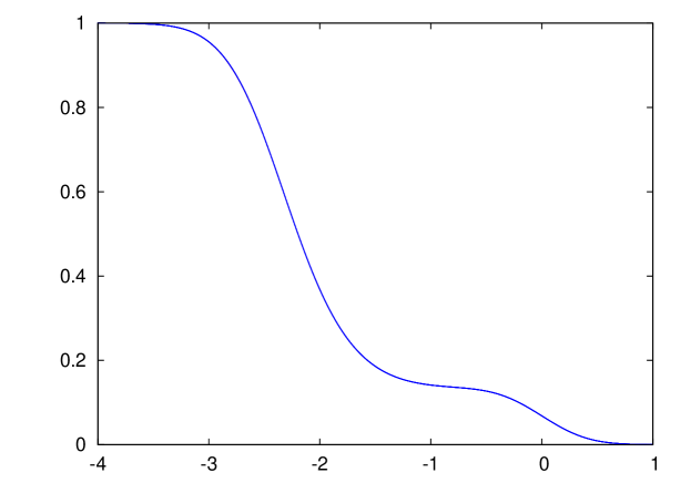
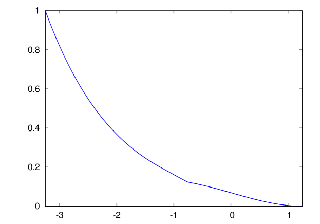
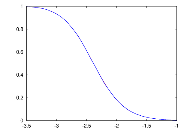
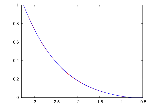
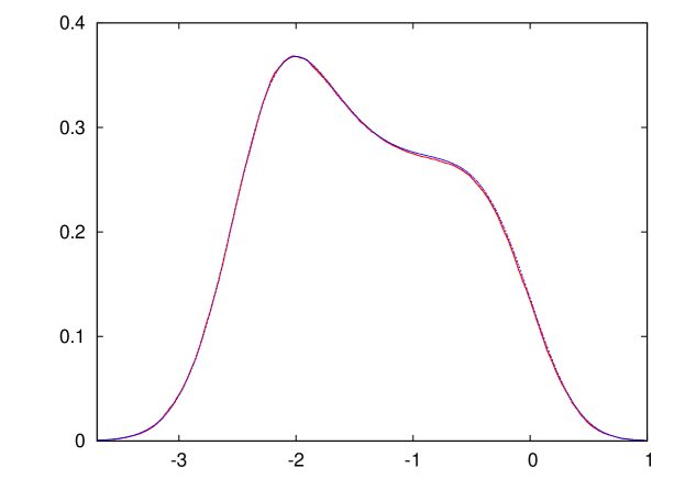
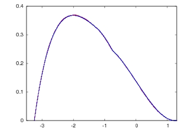
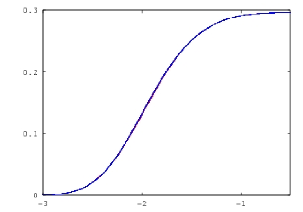
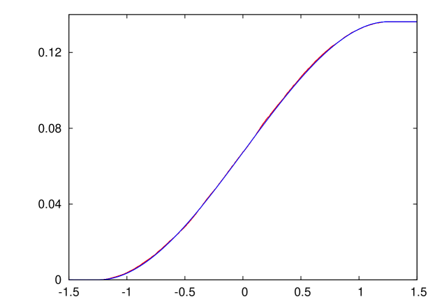
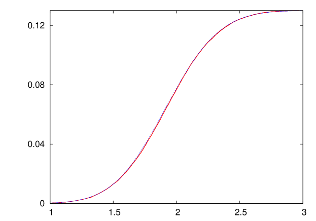
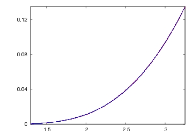
We begin with the probability per site of a doublet on the lower half of the hysteresis loop. Figure (18) shows the theoretical expression for $P_{\downarrow\downarrow}(h_{a})$ for the Gaussian distribution with the corresponding data from numerical simulation superimposed on it. The fit is so close that the two are indistinguishable on the scale of the figure. Figure (19) shows similar comparison for a uniform distribution with $\Delta=1.25$. In each of the following figures data from the corresponding numerical simulation has been plotted along side the theoretical expression. Even numbered figures are for the Gaussian distribution and the odd numbered figures for the uniform distribution. In some cases the match between theory and simulation is so good that there appears to be only a single curve in the figure. In other cases ( when the probability of the event is relatively small and finite size corrections are larger) we can barely make out that there are two curves that almost lie on each other. Figure(20) and figure (21) show the result for $P_{\downarrow\downarrow\downarrow}(h_{a})$ for the Gaussian and the uniform distribution respectively. Results for $P_{\uparrow\downarrow\downarrow}(h_{a})+P_{\downarrow\downarrow\uparrow}(h_{a})$ are shown in figures (22) and (23) for Gaussian and uniform distributions respectively. Figure (24) shows the comparison between theory and simulation for $P_{\uparrow\downarrow\uparrow A}(h_{a})$ in the case of Gaussian distribution. Figure (25) shows similar comparison for $P_{\uparrow\downarrow\uparrow D}(h_{a})$ for the uniform distribution. Figure (26) is for $P_{\uparrow\uparrow\uparrow M}(h_{a})$ for the Gaussian distribution. Figure (27) is for $P_{\uparrow\uparrow\uparrow N}(h_{a})$ for the rectangular distribution. Figures (28) and (29) each contain two objects. Figure (28) shows $P_{\uparrow\downarrow\uparrow Q}(h_{a})$ and $P_{\uparrow\uparrow\uparrow U}(h_{a})$ for Gaussian distribution. Figure (29) shows $P_{\uparrow\downarrow\uparrow R}(h_{a})$ and $P_{\uparrow\uparrow\uparrow V}(h_{a})$ for uniform distribution.

In conclusion we have obtained the zero-temperature hysteresis loop of a one dimensional anti-ferromagnetic random field Ising model in the case when the driving field varies from $-\infty$ to $\infty$ and back to $-\infty$ infinitely slowly. The problem is simple to state but difficult to solve. The theoretical result for the hysteresis loop involves integrals that have to be evaluated numerically in most cases. We have shown that our results fit numerical simulations of the model quite well. However, several aspects of the problem still remain unsolved. For example we have obtained the hysteresis loop when the driving field takes the system from one saturated state ($h_{a}=-\infty$) to another ($h_{a}=\infty$). In this case we have a complete knowledge of the statistical history of the system i.e. if a site is up at $h_{a}$, we know the relative probability of different sequence of events that result in this site being up. We are not in a position (so far) to obtain the hysteretic response of the system starting from an arbitrary initial state. It would be interesting to have an analytic solution of the problem in higher dimensions as well. Numerical simulations suggest that the anti-ferromagnetic hysteresis loops in higher dimensions have several plateaus for low values of $\Delta$ and $\sigma$ as compared with $|J|$. Exact analytic solutions of problems with quenched disorder are uncommon in statistical mechanics. One may even ask if they are worth the effort that has to be put in trying to obtain them. However exact solutions are intellectually satisfying and provide a framework for understanding a wide class of complex phenomena. We hope there will be more progress in this direction in the future.

Figure 1: Hysteresis loop for an anti-ferromagnetic random-field Ising model with $J=-1$ and $\Delta=0.5$ (see text). The $x$-axis shows the applied field and the $y$-axis magnetization per spin. As $|J|\leq\Delta$, each half of the hysteresis loop comprises three ramps separated by two plateaus. The lower half of the loop shows magnetization in increasing field and the upper half in decreasing field. A theoretical expression has been superimposed on the numerical data.

Figure 2: A magnified view of the theoretical and simulation hysteresis loops for $\Delta=0.5$ where the $y$-axis shows the magnetization in increasing and decreasing field as measured from the average of the magnetization on the lower and the upper half of the hysteresis loop in figure  1 at corresponding applied field.

Figure 3: Hysteresis loop for an anti-ferromagnetic random-field Ising model with $J=-1$ and $\Delta=1.25$ (see text). The $x$-axis shows the applied field and the $y$-axis magnetization per spin. As $|J|>\Delta$, the plateaus of figure  1 disappear and the three ramps merge into each other. A theoretical expression has been superimposed on the numerical data.

Figure 4: Theoretical and simulation hysteresis loops for $\Delta=1.25$ where the magnetization along increasing and decreasing field is measured from the average of the magnetization on the lower and the upper half of the hysteresis loop in figure  3 at corresponding applied field.

Figure 5: Hysteresis loop for an anti-ferromagnetic random-field Ising model with $J=-1$ and $\sigma=0.5$ (see text). Notice the approximate similarity with the hysteresis loop in figure  1 but the absence of sharp ramps and plateaus. For a Gaussian distribution the three ramps merge into each other for any value of $\sigma$ although this is less pronounced at smaller values of $\sigma$. A theoretical expression has been superimposed on the numerical data.

Figure 6: Magnified theoretical and simulation hysteresis loops for $\sigma=0.5$ where the magnetization along increasing and decreasing field is measured from the average of the magnetization on the lower and the upper half of the hysteresis loop in figure  5 at corresponding applied field.

Figure 7: Spins on Ramp-I in an applied field $-2|J|-h$. Filled circles show sites with quenched field $h_{i}>h$. The probability per site of a doublet (two adjacent down spins) such as AB is equal to $e^{-2p}$, where p is the fraction of filled circles on the infinite lattice.

Figure 8: A doublet on Plateau-I: $h_{1}$ and $h_{2}$ are the quenched random fields on the doublet sites 1 and 2 respectively.

Figure 9: Two adjacent doublets on Plateau-I: Each doublet separates the lattice into two parts whose evolution histories on Ramp-I are independent of each other. Evolutions inside each dashed box is shielded from outside. The probability that spin at site 3 flips up on Ramp-I is therefore equal to $\frac{1}{3}$. Given this, the probability that the spins at sites 1 and 5 remain down all along Ramp-I is equal to $\frac{1}{e}$ each. The shielding property of the boxes can also be used to determine a posteriori distribution of random fields $h_{1},h_{2},h_{3},h_{4},\mbox{ and }h_{5}$.

Figure 10: A singlet (site 3) with one next nearest neighbor down (site 1), and one next nearest neighbor up (site 5). When the singlet turns up at an applied field $h_{a}$, the spin at site 2 stays up if $\Delta\leq|J|$, but the spin at site 4 flips down if $h_{4}\leq h_{3}$.

Figure 11: Two adjacent singlets on Plateau-I: If $h_{2}=\mbox{min}(h_{2},h_{4})$, and $h_{3}\leq h_{2}$, then the spin at site 3 will flip down when the spin at site 2 flips up on ramp-III. This process creates a new singlet on ramp-III.

Figure 12: A singlet followed by a doublet on Plateau-I: If $h_{4}\geq h_{5}$, and $h_{3}\leq h_{2}$, then a new singlet will be created at site 3 when the spin at site 2 turns up on ramp-III.

Figure 13: A doublet followed by a singlet on Plateau-I: If $h_{3}\geq h_{2}$, and $h_{4}\leq h_{5}$, then a new singlet will be created at site 4 when the spin at site 5 turns up on ramp-III.

Figure 14: An up spin followed by a doublet. Site-1 may have flipped up under a $p_{0}$-process or a $p_{1}$-process. Subsequently when site-3 flips up we get a singlet at site-2. The fraction of such singlets depends on the details of how sites 1 and 3 have flipped.

Figure 15: A doublet followed by a doublet. We get a singlet at site-3 if sites 2 and 4 flip up before sites 1 and 5 and site-3 flips down because it is unstable with both neighbors up.

Figure 16: A singlet followed by a singlet. A singlet is created at site-3 if sites 2 and 4 flip up under a $p_{2}$-process and then site-3 flips down because it is unstable when both neighbors are up.

Figure 17: A doublet followed by a singlet. We get a singlet at site-3 if site-2 flips up under a $p_{1}$-process, site-4 flips up under a $p_{2}$-process and then site-3 flips down because it is unstable when both neighbors are up.

Figure 18: Probability of a doublet $P_{\downarrow\downarrow}(h_{a})$ for a Gaussian distribution with $\sigma=0.5|J|$. Simulation data has been superimposed on the theoretical expression.

Figure 19: Probability of a doublet $P_{\downarrow\downarrow}(h_{a})$ for a uniform distribution with $\Delta=1.25|J|$. Simulation data has been superimposed on the theoretical expression.

Figure 20: Probability of $P_{\downarrow\downarrow\downarrow}(h_{a})$ for a Gaussian distribution with $\sigma=0.5|J|$. Simulation data has been superimposed on the theoretical expression.

Figure 21: Probability of $P_{\downarrow\downarrow\downarrow}(h_{a})$ for a uniform distribution with $\Delta=1.25|J|$. Simulation data has been superimposed on the theoretical expression.

Figure 22: $P_{\uparrow\downarrow\downarrow}(h_{a})+P_{\downarrow\downarrow\uparrow}(h_{a})$ for a Gaussian distribution with $\sigma=0.5|J|$. Simulation data has been superimposed on the theoretical expression.

Figure 23: $P_{\uparrow\downarrow\downarrow}(h_{a})+P_{\downarrow\downarrow\uparrow}(h_{a})$ for a uniform distribution with $\Delta=1.25|J|$. Simulation data has been superimposed on the theoretical expression.

Figure 24: Theory and simulation for $P_{\uparrow\downarrow\uparrow A}(h_{a})$ for a Gaussian distribution with $\sigma=0.5|J|$.

Figure 25: Theory and simulation for $P_{\uparrow\downarrow\uparrow D}(h_{a})$ for a uniform distribution with $\Delta=1.25|J|$.

Figure 26: Theory and simulation for $P_{\uparrow\uparrow\uparrow M}(h_{a})$ for a Gaussian distribution with $\sigma=0.5|J|$.

Figure 27: Theory and simulation for $P_{\uparrow\uparrow\uparrow N}(h_{a})$ for a uniform distribution with $\Delta=1.25|J|$.

Figure 28: Theory and simulation for $P_{\uparrow\downarrow\uparrow Q}(h_{a})$ on the left, and $P_{\uparrow\uparrow\uparrow U}(h_{a})$ on the right for a Gaussian distribution with $\sigma=0.5|J|$.

Figure 29: Theory and simulation for $P_{\uparrow\downarrow\uparrow R}(h_{a})$ on the left, and $P_{\uparrow\uparrow\uparrow V}(h_{a})$ on the right for a uniform distribution with $\Delta=1.25|J|$.

References

- (1) See for example, The Science of Hysteresis, edited by G Bertotti and I Mayergoyz, Academic Press, Amsterdam (2006).
- (2) Spinglasses and Random Fields, ed. A P Young, World Scientific, Singapore (1997).
- (3) J P Sethna, K A Dahmen, S Kartha, J A Krumhansl, B W Roberts, and J D Shore, Phys Rev Lett 70, 3347 (1993); K Dahmen and J P Sethna, Phys Rev Lett 71, 3222(1993); O Perkovic, K Dahmen, and J P Sethna, Phys Rev Lett 75, 4528 (1995).
- (4) J P Sethna, K A Dahmen, and O. Percovic in bertotti and references therein.
- (5) K A Dahmen and J P Sethna, Phys Rev B 53, 14872 (1996).
- (6) Y Imry and S Ma Phys Rev Lett 35, 1399 (1975); for a more recent review of random field phenomena see e.g. T Nattermann in young .
- (7) R J Glauber, J Math Phys 4, 294 (1963).
- (8) K G Wilson, Phys Rev B4, 3174(1971); K G Wison, Phys Rev B4, 3184 (1971).
- (9) See for example, E C Stoner, Rev Mod Phys 25, 2 (1953). The main features of Barkhausen noise discovered in these early experiments are still topics of current research.
- (10) Hysteresis in an Ising chain with quenched random disorder, P Shukla, Prog Theo Phys 96, 69-80 (1996).
- (11) Exact solution of zero-temperature hysteresis in a ferromagnetic Ising chain with quenched random fields, P Shukla, Physica A233, 235-241 (1996).
- (12) D Dhar, P Shukla, and J P Sethna, J Phys A30, 5259 (1997).
- (13) S Sabhapandit, D Dhar, and P Shukla, Phys Rev Lett 88, 197202 (2002).
- (14) R da Silveira and M Kardar, Phys Rev E 59, 1355 (1999).
- (15) R A da Silveira and S Zapperi, Phys Rev B 69, 212404 (2004).
- (16) Hysteresis in random-field XY and Heisenberg models: Mean-field theory and simulations at zero temperature, Prabodh Shukla and R S Kharwanlang, Phys Rev E 81, 031106 (2010); cond-mat arXiv:0907.1957v2
- (17) Critical hysteresis in random-field XY and Heisenberg models, Prabodh Shukla and R S Kharwanlang, Phys Rev E 83, 011121 (2011); cond-mat arXiv:1007.4265v2
- (18) Zero-temperature hysteresis in an anti-ferromagnetic Ising chain with quenched random fields, P Shukla, Physica A233, 242-252 (1996).
- (19) Hysteretic response of an anti-ferromagnetic random field Ising model in one dimension at zero temperature, Prabodh Shukla, Ratnadeep Roy, and Emilia Ray, Physica A 275, 380 (2000); cond-mat/9910021.
- (20) item Hysteresis in one-dimensional anti-ferromagnetic random field Ising model at zero temperature, Prabodh Shukla, Ratnadeep Roy, and Emilia Ray, Physica A 276, 365 (2000); cond-mat/9910169.
- (21) Driven Random Field Ising Model: some exactly solved examples in threshold activated kinetics, Prabodh Shukla, Int J Mod Phys B 17, 5583 (2003); cond-mat/0401252.
- (22) Exact solution of return hysteresis loops in a one dimensional random-field Ising model at zero temperature, Prabodh shukla, Phys Rev E 62, 4725 (2000); cond-mat/0004125.
-
(23)
Exact expressions for minor hysteresis loops in the
random-field Ising model on a Bethe lattice at zero temperature, Prabodh
Shukla, Phys Rev E 63, 27102 (2001);
cond-mat/0007370. - (24) S Sabhapandit, P Shukla, and D Dhar, J Stat Phys 98, 103 (2000).
- (25) X Illa, P Shukla, and E Vives, Phys Rev B 73, 092414 (2006).
- (26) X Illa, M L Rosinberg, P Shukla, and E Vives, Phys Rev B 74, 224404 (2006).
- (27) X Illa, M L Rosinberg, and G Tarjus, Eur Phys J B54, 355 (2006).
- (28) P Ayyub et al, Phys Rev B 57, R5559 (1998).
- (29) K Fukuma and M Torii, Earth Planets Space 50, 9 (1998).
- (30) I Chiorescu et al, Phys Rev Lett 84, 3454 (2000).
- (31) E E Fullerton et al, Appld Phys Lett 77, 3806(2000).
- (32) O Waldmann et al, Phys Rev Lett 89, 246401(2002).
- (33) K Takanashi, Appld Phys Lett 63, 1585 (1993).
- (34) Khian-Hooi Chew et al, Appld Phys Lett 77, 2755 (2000).
- (35) J Kisker,H Rieger, and H Schreckenberg, J Phys A: Math. Gen. 27, L853 (1994). This paper discusses the non-equilibrium dynamics of a non-random, one-dimensional Ising model, with three-spin interactions, at low temperatures. It is qualitatively similar to the dynamics of the random field Ising model at zero-temperature.
- (36) H Reiger, Physica A 224, 267 (1996).
- (37) F Ritort and P Sollich, Advances in Physics 52:4, 219 (2003).
- (38) C Toninelli, PhD thesis (2003).
- (39) J W Evans, Rev Mod Phys 65, 1281 (1993).
- (40) L G Mityushin, Prob Peredachi Inf 9, 81 (1973). Also see reference (39) for a detailed discussion of the screening property of this class of problems.