Kumaraswamy and beta distribution are related by the logistic map

Abstract

The Kumaraswamy distribution has been proposed as an alternative to the beta distribution with more benign algebraic properties. They have the same two parameters, the same support and qualitatively similar shape for any parameter values. There is a generic relationship between the distributions established by a simple transformation between arbitrary Kumaraswamy-distributed random variables and certain beta-distributed random variables. Here, a different relationship is established by means of the logistic map, the paradigmatic example of a discrete non-linear dynamical system.

Keywords: Kumaraswamy distribution; Beta distribution; Logistic map

1 Introduction

1.1 The Logistic Map

The logistic map is a parametric discrete-time non-linear dynamical system. It is widely studied because of its complex transition from orderly to chaotic behavior in spite of an extremely simple defining equation (May, 1976).

Definition 1 (Logistic map).

For a real parameter $r>0$, the logistic map is the function

$$f_{r}(x)=rx(1-x)$$ (1)

restricted to the closed real interval $[0,1]$. This is a total function for $r\leq 4$.

The objects of interest are the trajectories that arise from the iteration of $f_{r}$, i.e., sequences with the recurrence relation $x_{n+1}=f_{r}(x_{n})$. With increasing $r$, they show all kinds of behavior from convergence in a singular attractor through bifurcating periodic solutions to deterministic chaos. The case $r=4$ is of special interest: It is known to be chaotic and ergodic on the interval $[0,1]$. The density of the attractor is given by the beta distribution with parameters $\alpha=\beta=1/2$ and hence, by ergodicity, the long-term distribution of states under almost all initial conditions (with the exception of unstable periodic solutions) converges to that distribution (Jakobson, 1981).

1.2 The Kumaraswamy Distribution

Kumaraswamy (1980) introduced his now eponymous distribution, originally called double-bounded distribution, as an alternative to the beta distribution. They have the same real parameters $\alpha,\beta>0$, the same support and similar shapes, but the Kumaraswamy distribution function, unlike the beta distribution function, has a closed algebraic form. Is has been found both more accurately fitting hydrological data in simulations (Kumaraswamy, 1980) and computationally more tractable (Jones, 2009).

The similarity between the two classes can be formalized. It is known and easy to see (from equations (3) and (6) below) that, if random variable $X$ is Kumaraswamy-distributed with parameters $\alpha$ and $\beta$, then $X^{\alpha}$ is beta-distributed with $\alpha=1$ and the same $\beta$. Here, a new formal relationship between certain beta and Kumaraswamy distributions is established.

2 Computing State Distributions of the Logistic Map

Given a random variable $X$ with known distribution on $[0,1]$, the propagated distribution of $f_{r}(X)$ can be computed. In the following, the term continuous probability distribution (cdf) refers to a cumulative distribution function with support $[0,1]$, that is, a continuous weakly monotonic function $F:[0,1]\to[0,1]$ with $F(0)=0$ and $F(1)=1$. A random variable $X$ is distributed according to $F$, written $X\sim F$, if and only if $P(X\leq y)=P(X<y)=F(y)$.

Definition 2 (Propagation).

Let $F$ be a cdf. Then $\widetilde{f}_{r}(F)$ is another cdf, namely

$$\widetilde{f}_{r}(F)(y)=F\bigl{(}\tfrac{1}{2}-q_{r}(y)\bigr{)}+1-F\bigl{(}\tfrac{1}{2}+q_{r}(y)\bigr{)}\,,$$ (2a)

where

$$q_{r}(y)=\begin{cases}\sqrt{\tfrac{1}{4}-\tfrac{y}{r}}&\text{if }y\leq\tfrac{r}{4}\\ 0&\text{if }y>\tfrac{r}{4}\,.\end{cases}$$ (2b)

Theorem 1.

If $X\sim F$ then $f_{r}(X)\sim\widetilde{f}_{r}(F)$.

Proof.

$$P(f_{r}(X)\leq y\bigr{)} =P\bigl{(}rx(1-x)\leq y)$$

$$=P\bigl{(}\bigl{(}x-\tfrac{1}{2}\bigr{)}^{2}\geq\tfrac{1}{4}-\tfrac{y}{r}\bigr{)}$$

$$=P\bigl{(}\bigl{\lvert}x-\tfrac{1}{2}\bigr{\rvert}\geq q_{r}(y)\bigr{)}$$

$$=P\bigl{(}x\leq\tfrac{1}{2}-q_{r}(y)\lor x\geq\tfrac{1}{2}+q_{r}(y)\bigr{)}$$

$$=P\bigl{(}x\leq\tfrac{1}{2}-q_{r}(y)\bigr{)}+P\bigl{(}x\geq\tfrac{1}{2}+q_{r}(y)\bigr{)}$$

$$=P\bigl{(}x\leq\tfrac{1}{2}-q_{r}(y)\bigr{)}+1-P\bigl{(}x\leq\tfrac{1}{2}+q_{r}(y)\bigr{)}$$

$$=F\bigl{(}\tfrac{1}{2}-q_{r}(y)\bigr{)}+1-F\bigl{(}\tfrac{1}{2}+q_{r}(y)\bigr{)}$$

$$=\widetilde{f}_{r}(F)(y)$$

∎

The beta distribution with real parameters $\alpha,\beta>0$ has the cdf

$$B(\alpha,\beta)(y)=\int_{0}^{y}t^{\alpha-1}(1-t)^{\beta-1}dt\Bigm{/}\int_{0}^{1}t^{\alpha-1}(1-t)^{\beta-1}dt\,.$$ (3)

For $\alpha=\beta=1/2$ the beta distribution is the arcsine distribution.

$$B(1/2,1/2)(y)=A(y)=2/\pi\arcsin\sqrt{y}$$ (4)

Theorem 2.

The arcsine distribution is a fixed point of $\widetilde{f}_{4}$.

Proof.

Using the symmetry of (4) and the trigonometric identity

$$\arcsin\sqrt{y}=2\arcsin\sqrt{\frac{1-\sqrt{1-y}}{2}}\,,$$ (5)

one finds that

$$\widetilde{f}_{4}(A)(y) =2A\bigl{(}\tfrac{1}{2}-q_{4}(y)\bigr{)}=2A\left(\frac{1-\sqrt{1-y}}{2}\right)=A(y)\,.$$

∎

The uniform distribution has the cdf $U(y)=y$. The Kumaraswamy distribution with real parameters $\alpha,\beta>0$ has the cdf

$$K(\alpha,\beta)(y)=1-(1-y^{\alpha})^{\beta}\,.$$ (6)

Theorem 3.

Let $X$ be distributed uniformly. Then $f_{4}{}^{2}(X)=f_{4}\bigl{(}f_{4}(X)\bigr{)}$ is Kumaraswamy-distributed with $\alpha=\beta=1/2$.

$$\widetilde{f}_{4}{}^{2}(U)=K\bigl{(}\tfrac{1}{2},\tfrac{1}{2}\bigr{)}$$ (7)

Proof.

For $r=4$, (2b) simplifies to $q_{4}(y)=\sqrt{1-y}/2$ and hence (2a) to

$$\widetilde{f}_{4}(F)(y)=F\left(\frac{1-\sqrt{1-y}}{2}\right)+1-F\left(\frac{1+\sqrt{1-y}}{2}\right)\,.$$

Then after one step one has

$$\widetilde{f}_{4}(U)(y) =\frac{1-\sqrt{1-y}}{2}+1-\frac{1+\sqrt{1-y}}{2}=1-\sqrt{1-y}\,,$$

such that $\widetilde{f}_{4}(U)=K(1,1/2)$, and after two steps one has

$$\widetilde{f}_{4}{}^{2}(U)(y) =\widetilde{f}_{4}\bigl{(}\widetilde{f}_{4}(U)\bigr{)}(y)$$

$$=\widetilde{f}_{4}(U)\left(\frac{1-\sqrt{1-y}}{2}\right)+1-\widetilde{f}_{4}(U)\left(\frac{1+\sqrt{1-y}}{2}\right)$$

$$=1-\underbrace{\left(\sqrt{\frac{1+\sqrt{1-y}}{2}}-\sqrt{\frac{1-\sqrt{1-y}}{2}}\right)}_{s}\,.$$

The term $s$ looks rather convoluted, but its square simplifies to $s^{2}=1-\sqrt{y}$, so with $s>0$ conclude that $s=\sqrt{1-\sqrt{y}}$. Hence from (6) follows (7):

$$\widetilde{f}_{4}{}^{2}(U)(y)=1-\sqrt{1-\sqrt{y}}=1-(1-y^{1/2})^{1/2}$$

and thus $\widetilde{f}_{4}{}^{2}(U)=K(1/2,1/2)$. ∎

3 Conclusion

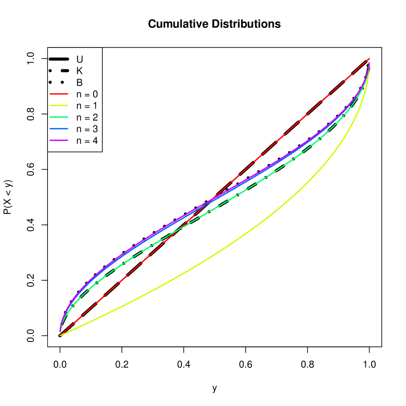
We have examined the probability distribution of successive states of the chaotic dynamical system described by the logistic map with parameter value $r=4$. It is known that this system is ergodic and that its long-term behavior is described by the beta$(1/2,1/2)$ distribution. Hence the distribution of states will converge almost surely. In order to investigate individual elements of that convergent sequence, we have given a closed formula for propagating probability distributions over the iteration of $f_{r}$ (Theorem 1), and validated this approach by demonstrating that the beta$(1/2,1/2)$ distribution is indeed a fixed point solution (Theorem 2). We have proceeded to demonstrate that, starting from the uniform distribution (the maximum-entropy distribution on the state space), after two steps the Kumaraswamy$(1/2,1/2)$ distribution is reached (Theorem 3). Figure 1 shows the cdfs of the initial state and the first four iterates plotted over the uniform, Kumaraswamy and beta distributions.

The above findings qualify as purely theoretical results in the sense that they provide original and provable insights about the relationship of mathematical objects of theoretical interest. No suggestion can be given yet as to the application to real-world statistical problems. Apart from the investigation of potential practical implications, the presentation of higher iterates $\widetilde{f}_{4}{}^{3}(U),\dots$ is an open problem. The initial sequence of distributions $\widetilde{f}_{4}{}^{n}(U)$ looks pretty regular:

$$\underbrace{U=B(1,1)=K(1,1)}_{n=0}~{}\longmapsto~{}\underbrace{K\bigl{(}1,\tfrac{1}{2}\bigr{)}}_{n=1}~{}\longmapsto~{}\underbrace{K\bigl{(}\tfrac{1}{2},\tfrac{1}{2}\bigr{)}}_{n=2}\,,$$

but there is no obvious continuation of the pattern for $n\geq 3$.

Figure 1: State cdfs $D_{n}=\widetilde{f}_{4}{}^{n}(U)$ of an initially uniformly distributed system running the logistic map with $r=4$, after $n=0,\dots,4$ steps; plotted over the uniform ($U$), Kumaraswamy ($K$) and beta ($B$) distributions, with parameters $\alpha=\beta=1/2$. $D_{0}$ coincides with $U$. $D_{2}$ coincides with $K$. For $n>3$, $D_{n}$ converges towards $B$.

References

• Jakobson [1981] M.V. Jakobson. Absolutely continuous invariant measures for one-parameter families of one-dimensional maps. Communications in Mathematical Physics, 81(1):39–88, 1981.
• Jones [2009] M.C. Jones. Kumaraswamy’s distribution: A beta-type distribution with some tractability advantages. Statistical Methodology, 6(1):70–81, 2009. ISSN 1572-3127. doi: 10.1016/j.stamet.2008.04.001.
• Kumaraswamy [1980] P.Β Kumaraswamy. A generalized probability density function for double-bounded random processes. Journal of Hydrology, 46(1–2):79–88, 1980. ISSN 0022-1694. doi: 10.1016/0022-1694(80)90036-0.
• May [1976] RobertΒ M. May. Simple mathematical models with very complicated dynamics. Nature, 261(5560):459–467, 1976.
Refer to caption
Figure 1: State cdfs Dn=f~4(U)nD_{n}=\widetilde{f}_{4}{}^{n}(U) of an initially uniformly distributed system running the logistic map with r=4π‘Ÿ4r=4, after n=0,…,4𝑛0…4n=0,\dots,4 steps; plotted over the uniform (Uπ‘ˆU), Kumaraswamy (K𝐾K) and beta (B𝐡B) distributions, with parameters Ξ±=Ξ²=1/2𝛼𝛽12\alpha=\beta=1/2. D0subscript𝐷0D_{0} coincides with Uπ‘ˆU. D2subscript𝐷2D_{2} coincides with K𝐾K. For n>3𝑛3n>3, Dnsubscript𝐷𝑛D_{n} converges towards B𝐡B.